Downloaded 108 times

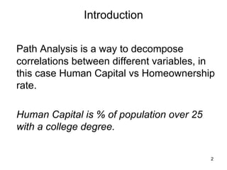
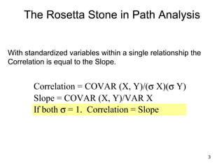
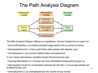
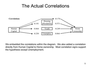
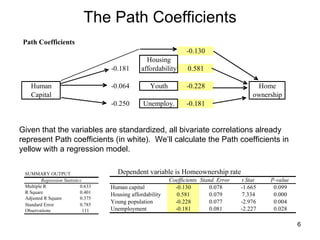
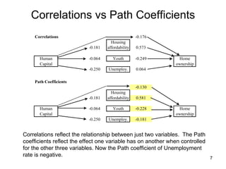
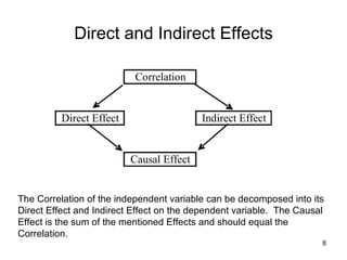
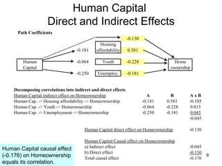
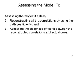
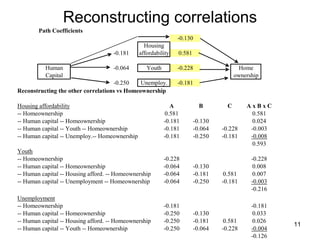
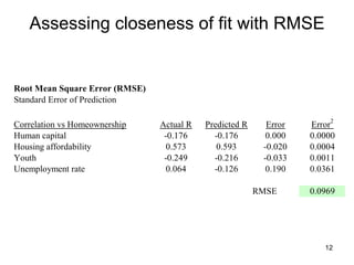

The document explores path analysis to examine the correlation between human capital, defined as the percentage of the population over 25 with a college degree, and homeownership rates. It discusses how human capital negatively influences home affordability and demographic youth while impacting unemployment. The analysis includes path coefficients and correlations to evaluate the effects of these variables on homeownership rates, assessing model fit and implications for further research.