Download as PDF, PPTX
![Dynamical
Systems
Methods in
Early-Universe
Cosmologies
Ikjyot Singh
Kohli
Ph.D.
Candidate
York
University
Outline
Introduction
Description of
the Matter
Deriving the
Dynamical
Equations
The Theory of
Orthonormal
Frames
Dynamical
Systems
Techniques
Motivation
In this presentation, we are concerned with applying
dynamical systems theory to get information about the
early universe.
The early universe, that is, shortly after the big bang was
a hot and dense place, and it is not necessarily true that
the perfect fluid description used in the standard
cosmological models today would hold in such conditions.
One has to account for potential anisotropic/dissipative
effects which in fluid dynamics as characterized by
viscosity.
For a review of the justification of including viscosity
terms in early-universe cosmological models see the
articles by Barrow (1988,1982) [3] [2] and the article by
Belinskii and Khalatnikov (1976) [4].](https://image.slidesharecdn.com/presentationisk-141218182637-conversion-gate01/75/Cosmology-Group-Presentation-at-York-University-6-2048.jpg)
![Dynamical
Systems
Methods in
Early-Universe
Cosmologies
Ikjyot Singh
Kohli
Ph.D.
Candidate
York
University
Outline
Introduction
Description of
the Matter
Deriving the
Dynamical
Equations
The Theory of
Orthonormal
Frames
Dynamical
Systems
Techniques
Motivation
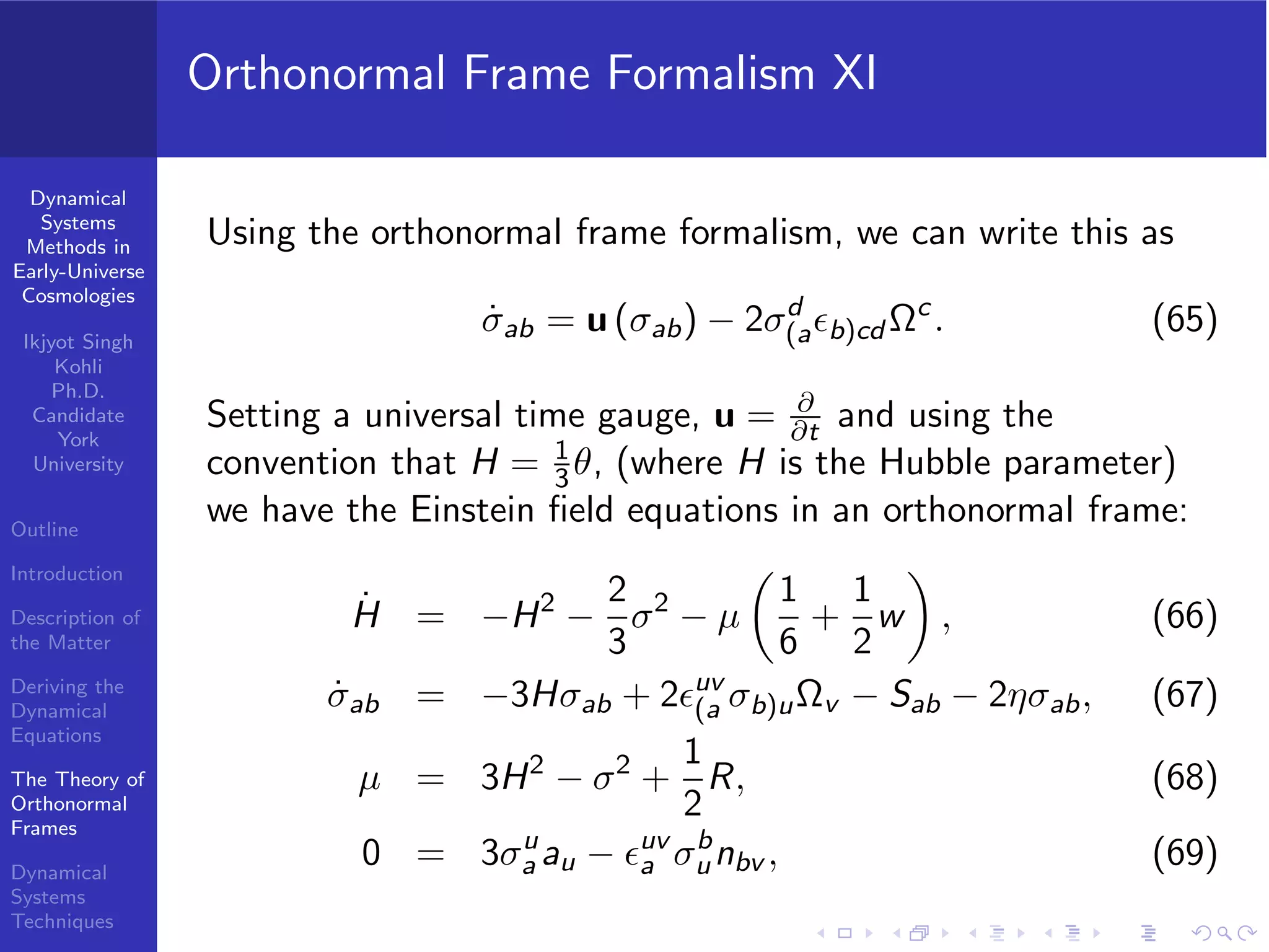
In this presentation, we are concerned with applying
dynamical systems theory to get information about the
early universe.
The early universe, that is, shortly after the big bang was
a hot and dense place, and it is not necessarily true that
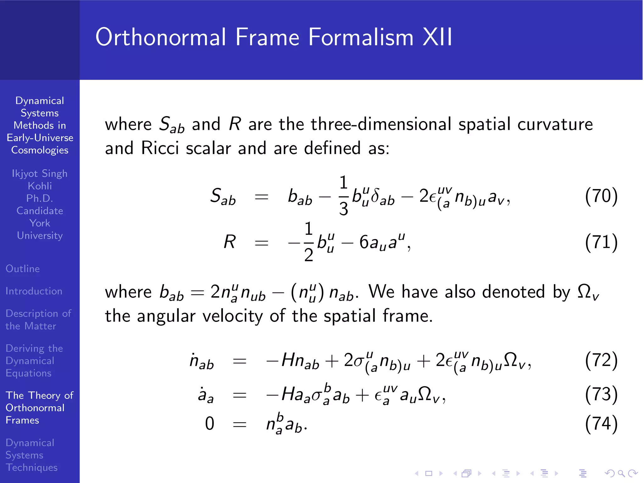
the perfect fluid description used in the standard
cosmological models today would hold in such conditions.
One has to account for potential anisotropic/dissipative
effects which in fluid dynamics as characterized by
viscosity.
For a review of the justification of including viscosity
terms in early-universe cosmological models see the
articles by Barrow (1988,1982) [3] [2] and the article by
Belinskii and Khalatnikov (1976) [4].
As a result, we will keep our assumption of the spatial
homogeneity of the early universe, but now assume it is](https://image.slidesharecdn.com/presentationisk-141218182637-conversion-gate01/75/Cosmology-Group-Presentation-at-York-University-7-2048.jpg)
![Dynamical
Systems
Methods in
Early-Universe
Cosmologies
Ikjyot Singh
Kohli
Ph.D.
Candidate
York
University
Outline
Introduction
Description of
the Matter
Deriving the
Dynamical
Equations
The Theory of
Orthonormal
Frames
Dynamical
Systems
Techniques
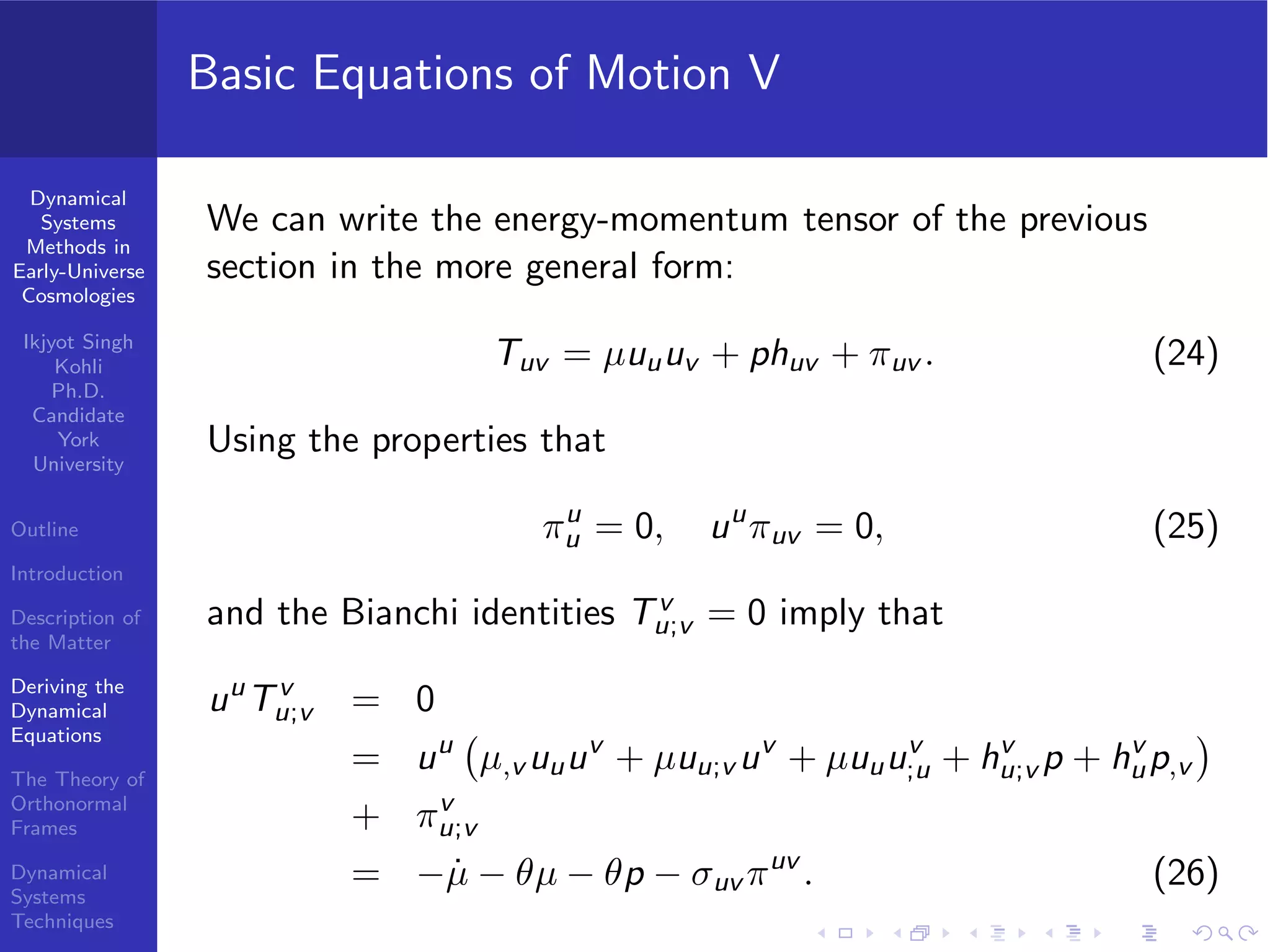
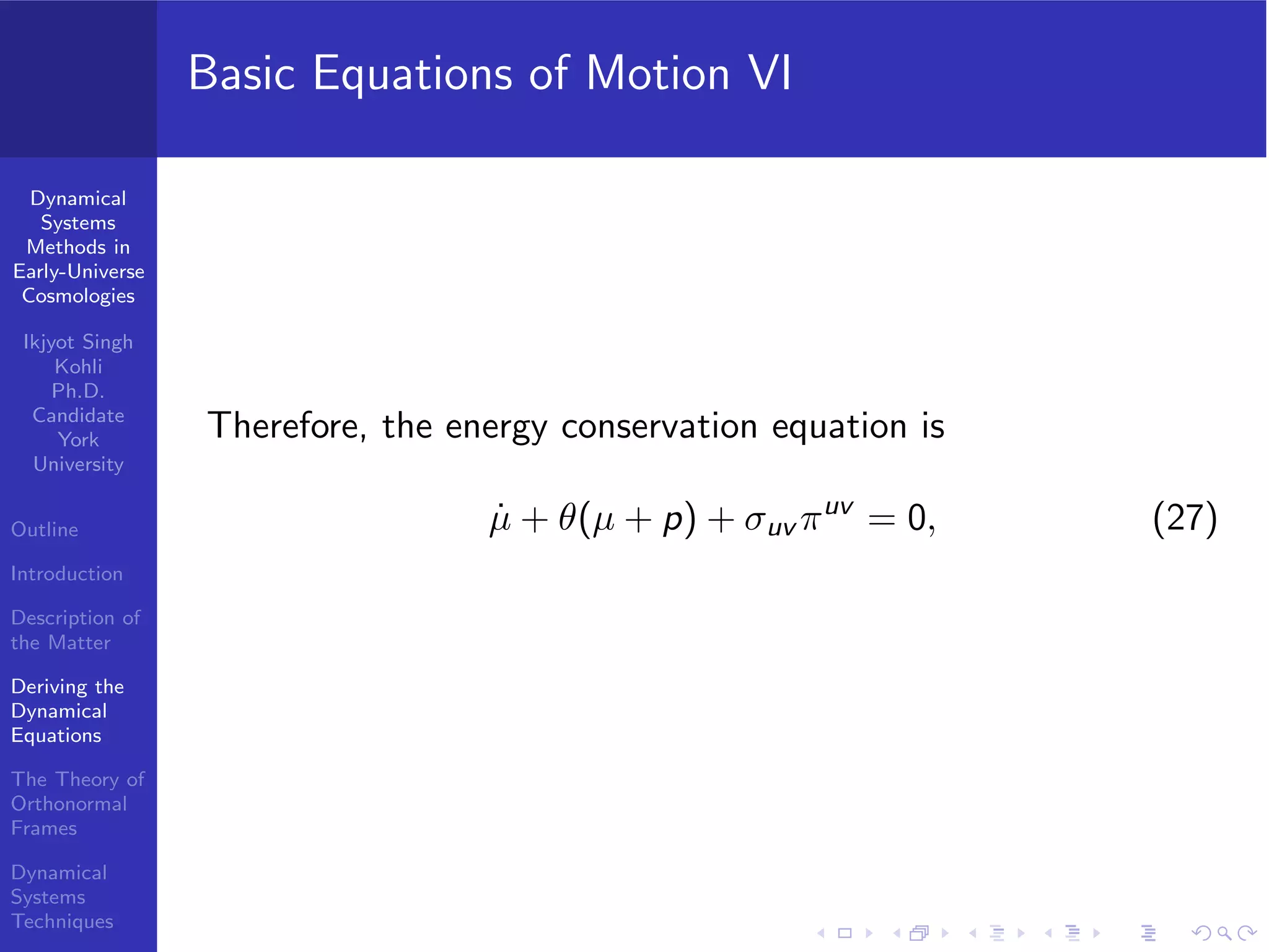
Energy-Momentum Tensor Derivation IV
Therefore, ˜Σik is some function of the ui,k. In addition,
when the fluid is in rotation, no internal motions of
particles can be occurring, so we consider linear
combinations of ui,k + uk,i , which clearly vanish for a fluid
in rotation with some angular velocity, Ωi . The most
general viscous tensor that can be formed is given by
˜Σik = η ui,k + uk,i −
2
3
δikul,l + ξδikul,l , (8)
where η and ξ are the coefficients of shear and
bulk/second viscosity, respectively [15] [13].](https://image.slidesharecdn.com/presentationisk-141218182637-conversion-gate01/75/Cosmology-Group-Presentation-at-York-University-11-2048.jpg)
![Dynamical
Systems
Methods in
Early-Universe
Cosmologies
Ikjyot Singh
Kohli
Ph.D.
Candidate
York
University
Outline
Introduction
Description of
the Matter
Deriving the
Dynamical
Equations
The Theory of
Orthonormal
Frames
Dynamical
Systems
Techniques
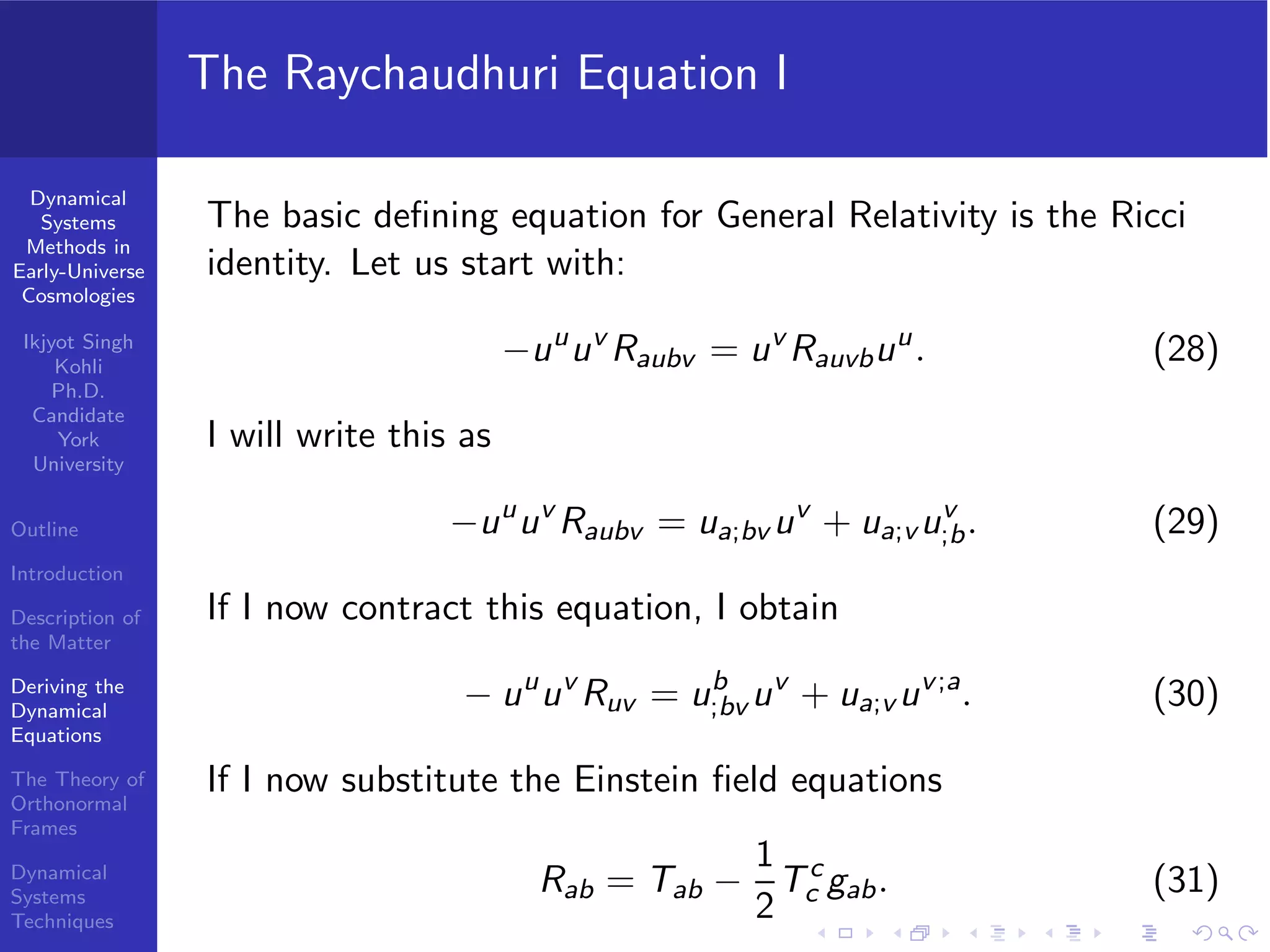
Basic Equations of Motion I
We will now derive the dynamical equations. Most of this
derivation follows from Ellis [6] and Grøn and Hervik [9], but I
have tried to make thing slightly easier to understand. Let us
first recall some basic properties of non-relativistic fluid
mechanics. In fluid mechanics, we typically measure the fluid
acceleration through the material derivative:
Dv
dt
≡ v,t + (v · ∇)v, (14)
where v,t is the local derivative, and (v · ∇)v is known as the
convective derivative. Note that
Dva
dt
= va
,t + va
,bxb
,t = va
,t + vb
va
,b. (15)](https://image.slidesharecdn.com/presentationisk-141218182637-conversion-gate01/75/Cosmology-Group-Presentation-at-York-University-14-2048.jpg)
![Dynamical
Systems
Methods in
Early-Universe
Cosmologies
Ikjyot Singh
Kohli
Ph.D.
Candidate
York
University
Outline
Introduction
Description of
the Matter
Deriving the
Dynamical
Equations
The Theory of
Orthonormal
Frames
Dynamical
Systems
Techniques
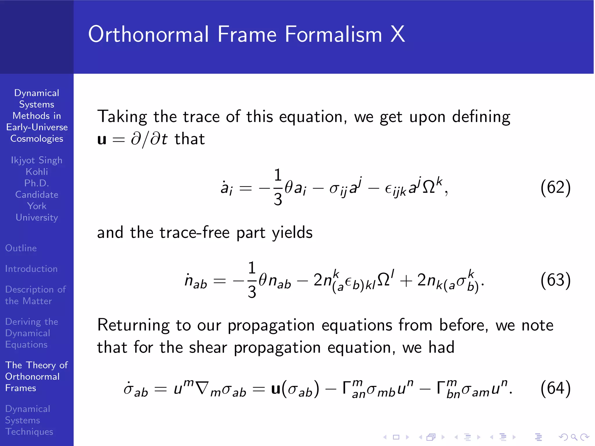
To close this system, we need dynamical equations for θ and
σuv . The idea for using kinematics to describe the dynamics of
universes obeying the Einstein field equations was first
introduced by Trumper as mentioned in Hawking’s 1966 paper
[10] and in Ellis’ Cargese Lectures [6].](https://image.slidesharecdn.com/presentationisk-141218182637-conversion-gate01/75/Cosmology-Group-Presentation-at-York-University-20-2048.jpg)
![Dynamical
Systems
Methods in
Early-Universe
Cosmologies
Ikjyot Singh
Kohli
Ph.D.
Candidate
York
University
Outline
Introduction
Description of
the Matter
Deriving the
Dynamical
Equations
The Theory of
Orthonormal
Frames
Dynamical
Systems
Techniques
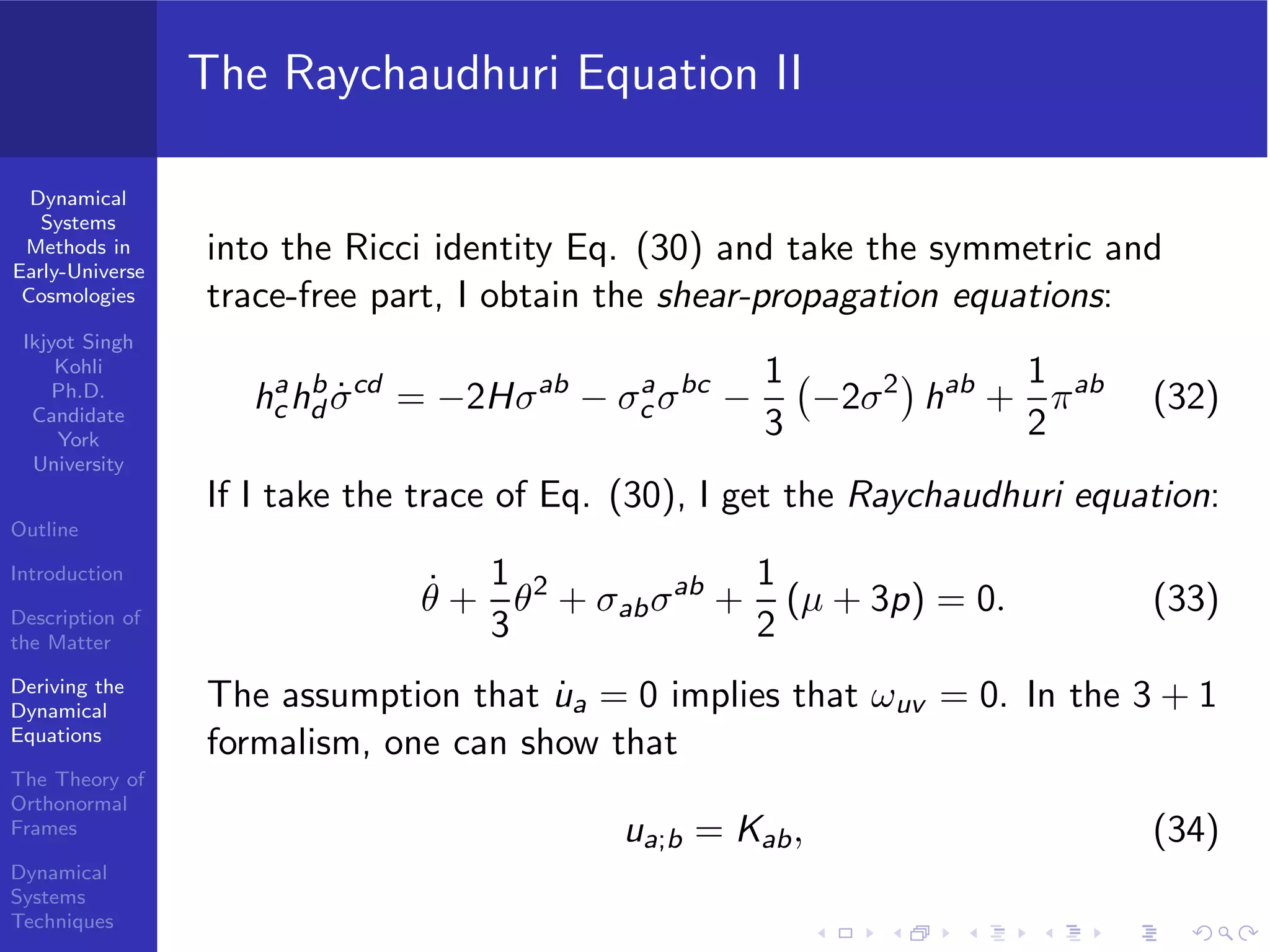
The Raychaudhuri Equation III
where Kab is the extrinsic curvature tensor. Gauss’ theorem
egregium (Page 171, [9]) states that
(n+1)
R =(n)
R + K2
− Kab
Kab + 2(−1)(n+1)
Rabua
ub
. (35)
Combining this with the Einstein field equations, we get:
Tab
uaub =
1
2
(3)
R − Kab
Kab + K2
. (36)
If we now use Eqs. (23) and (24), we get the Friedmann
equation:
1
3
θ2
=
1
2
σabσab
−
1
2
(3)
R + µ. (37)
This is a constraint equation on initial conditions as we will see
later.](https://image.slidesharecdn.com/presentationisk-141218182637-conversion-gate01/75/Cosmology-Group-Presentation-at-York-University-23-2048.jpg)
![Dynamical
Systems
Methods in
Early-Universe
Cosmologies
Ikjyot Singh
Kohli
Ph.D.
Candidate
York
University
Outline
Introduction
Description of
the Matter
Deriving the
Dynamical
Equations
The Theory of
Orthonormal
Frames
Dynamical
Systems
Techniques
Orthonormal Frame Formalism I
The idea of orthonormal frames is based on the groundbreaking
1969 paper from Ellis and MacCallum [8], “A Class of
Homogeneous Cosmological Models”. First, what do we mean
when we say a space-time is spatially homogeneous? Let M be
a manifold with metric tensor g. The isometry group is defined
by
Isom(M = {φ : M → M|φ, isometry}, (39)
that is φ∗g = g, i.e., the metric is left unchanged after applying
an isometry. This isometry group is a Lie group, and the group
generators are Killing vectors. These Killing vectors span a
finite-dimensional space (the tangent space to the Lie group),
and we define the isotropy subgroup of a point p ∈ M by
fp(M) = {φ ∈ Isom(M)|φ(p) = p}. (40)](https://image.slidesharecdn.com/presentationisk-141218182637-conversion-gate01/75/Cosmology-Group-Presentation-at-York-University-25-2048.jpg)
![Dynamical
Systems
Methods in
Early-Universe
Cosmologies
Ikjyot Singh
Kohli
Ph.D.
Candidate
York
University
Outline
Introduction
Description of
the Matter
Deriving the
Dynamical
Equations
The Theory of
Orthonormal
Frames
Dynamical
Systems
Techniques
Orthonormal Frame Formalism II
So a homogenous space is one that for each pair of points
a, b ∈ M, there exists a φ ∈ Isom(M) such that φ(p) = q.
For such a homogeneous space, there exists a set of Killing
vector fields ζi such that
[ζi , ζj ] = Dk
ij ζk. (41)
At a point p ∈ M, choose a basis set of vectors ei . It can be
shown that the frame ei span a Lie algebra:
[ei , ej ] = Ck
ij ek . (42)
Therefore, to construct a homogeneous space, one takes the
Ck
ij as the structure constants of the Lie algebra, and defines a](https://image.slidesharecdn.com/presentationisk-141218182637-conversion-gate01/75/Cosmology-Group-Presentation-at-York-University-26-2048.jpg)
![Dynamical
Systems
Methods in
Early-Universe
Cosmologies
Ikjyot Singh
Kohli
Ph.D.
Candidate
York
University
Outline
Introduction
Description of
the Matter
Deriving the
Dynamical
Equations
The Theory of
Orthonormal
Frames
Dynamical
Systems
Techniques
Orthonormal Frame Formalism IV
Now define
uv(g) = um
em(vn
en(g)), (46)
which is
uv(g) = um
em(vn
)en(g) + um
un
emen(g). (47)
This is clearly not a vector, since it has second-order partial
derivatives. However,
[u, v] = [um
em(vn
) − vm
em(un
)] en + um
un
[em, en] (48)
is indeed a vector. For an arbitrary basis,
[em, en] = cp
uv ep. (49)
These structure coefficients obviously vanish in a coordinate
basis, which is what most cosmologists usually work in.](https://image.slidesharecdn.com/presentationisk-141218182637-conversion-gate01/75/Cosmology-Group-Presentation-at-York-University-28-2048.jpg)
![Dynamical
Systems
Methods in
Early-Universe
Cosmologies
Ikjyot Singh
Kohli
Ph.D.
Candidate
York
University
Outline
Introduction
Description of
the Matter
Deriving the
Dynamical
Equations
The Theory of
Orthonormal
Frames
Dynamical
Systems
Techniques
Orthonormal Frame Formalism V
We will also make use of a generalized connection ∇ that
associates ∇XY to any two vector fields X and Y. In a general
basis, we have that
∇v em = Γa
mnea, (50)
that is, the connection coefficients are defined as the
components of the directional derivative of the basis vectors.
For more information, see [9] and Abraham and Marsden’s
book [1]. For two vector fields, X = Xmem, and u = umem, we
have that
∇uX = (en(Xm
)un
+ Xa
Γm
anuv
) em. (51)
The commutator above therefore can now be written as:
[u, v] = ∇uv − ∇vu + (Γp
mn − Γp
nm + cp
mn) um
un
ep. (52)](https://image.slidesharecdn.com/presentationisk-141218182637-conversion-gate01/75/Cosmology-Group-Presentation-at-York-University-29-2048.jpg)
![Dynamical
Systems
Methods in
Early-Universe
Cosmologies
Ikjyot Singh
Kohli
Ph.D.
Candidate
York
University
Outline
Introduction
Description of
the Matter
Deriving the
Dynamical
Equations
The Theory of
Orthonormal
Frames
Dynamical
Systems
Techniques
Orthonormal Frame Formalism VI
We defined the Torsion to be
ˆT(u ∧ v) ≡ ∇uv − ∇vu − [u, v] . (53)
We require spacetime in General Relativity to be torsion-free,
so we have
ca
mn = Γa
nm − Γa
mn. (54)
That is, all of the connection coefficients are now functions of
the structure constants!
In an orthonormal basis, gab = diag(−1, 1, 1, 1), so
Γamn =
1
2
gabcb
nm + gmbcb
an − gnbcb
ma . (55)
These are antisymmetric in the first two indices, so we can
write:
Γabt = −Γbat ≡ ϵabcΩc
, (56)](https://image.slidesharecdn.com/presentationisk-141218182637-conversion-gate01/75/Cosmology-Group-Presentation-at-York-University-30-2048.jpg)
![Dynamical
Systems
Methods in
Early-Universe
Cosmologies
Ikjyot Singh
Kohli
Ph.D.
Candidate
York
University
Outline
Introduction
Description of
the Matter
Deriving the
Dynamical
Equations
The Theory of
Orthonormal
Frames
Dynamical
Systems
Techniques
Orthonormal Frame Formalism VII
where Ωc denotes the rotation of the spatial frame and is
defined by
Ωa
=
1
2
ϵabgd
ubeg · ˙ed . (57)
We can therefore write that
ca
tb = −θa
b + ϵa
bcΩc. (58)
The rest of the structure coefficients are all spatial in nature,
and we can write
ck
ij = ϵijl nlk
+ al δk
i δl
j − δk
j δl
i , (59)
where nlk and ai classify the Bianchi algebra, per the Behr
decomposition (See Stephani, Kramer, MacCallum,
Hoenselaers, and Herit [16]), Landau and Liftshitz [14], Grøn
and Hervik [9] for a further explanation:](https://image.slidesharecdn.com/presentationisk-141218182637-conversion-gate01/75/Cosmology-Group-Presentation-at-York-University-31-2048.jpg)
![Dynamical
Systems
Methods in
Early-Universe
Cosmologies
Ikjyot Singh
Kohli
Ph.D.
Candidate
York
University
Outline
Introduction
Description of
the Matter
Deriving the
Dynamical
Equations
The Theory of
Orthonormal
Frames
Dynamical
Systems
Techniques
Orthonormal Frame Formalism IX
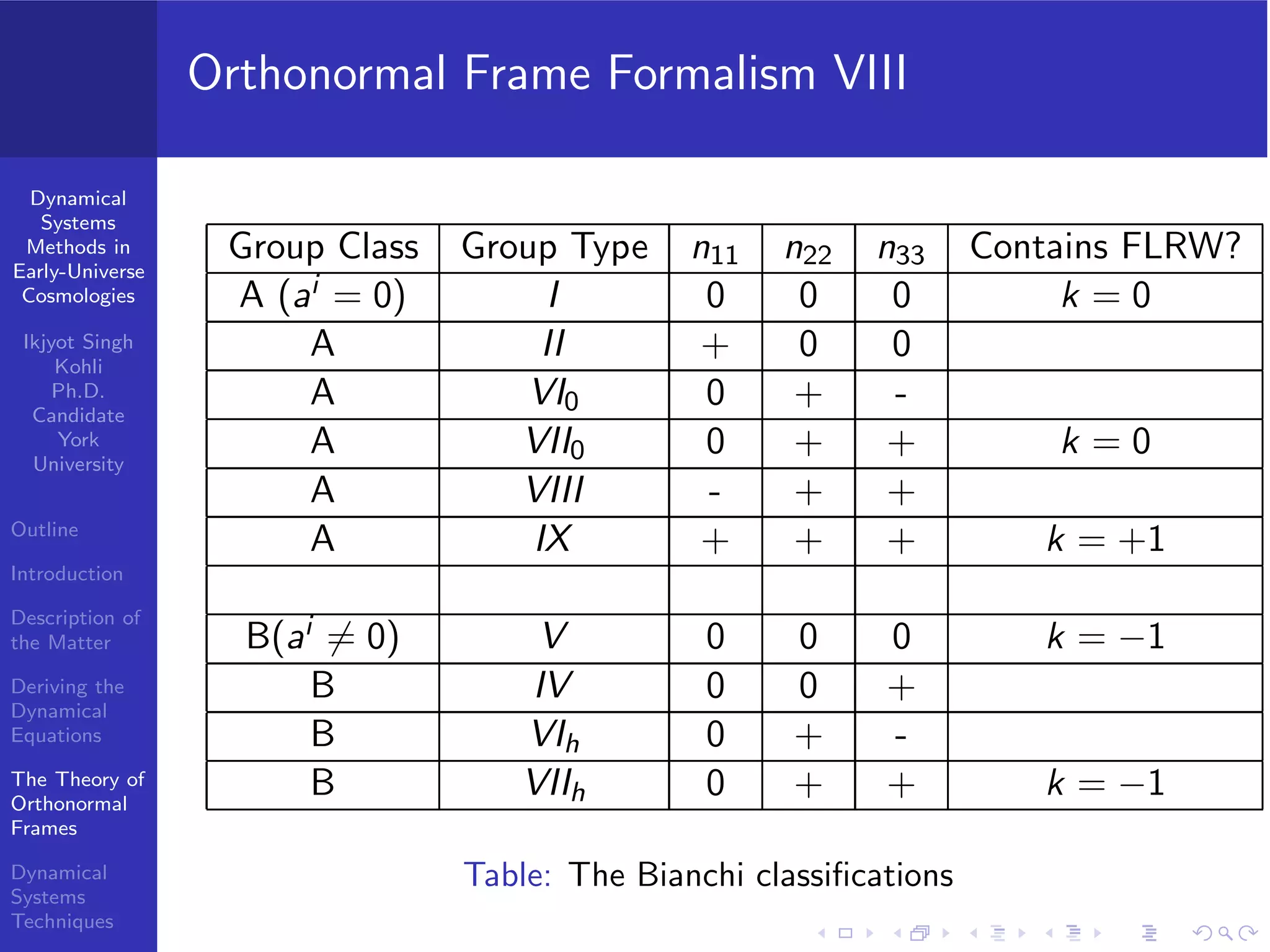
These classifications were due to Bianchi [5], but we follow the
conventions of Ellis, Maartens and MacCallum. [7].
One can find evolution equations for the nlk and the ai by
recognizing that the structure coefficients define a Lie algebra,
so that the Jacobi identity holds. That is, for the set of vectors
(u, ea, eb), we have that
0 = [u, [ea, eb]] + [ea, [eb, u]] + [eb, [u, ea]]. (60)
Go through some algebra, actually a lot of algebra (!), and find
that we get
u(ck
ab) + ck
td cd
ab + ck
ad cd
bt + ck
bd cd
ta = 0. (61)](https://image.slidesharecdn.com/presentationisk-141218182637-conversion-gate01/75/Cosmology-Group-Presentation-at-York-University-33-2048.jpg)
![Dynamical
Systems
Methods in
Early-Universe
Cosmologies
Ikjyot Singh
Kohli
Ph.D.
Candidate
York
University
Outline
Introduction
Description of
the Matter
Deriving the
Dynamical
Equations
The Theory of
Orthonormal
Frames
Dynamical
Systems
Techniques
Dynamical Systems Methods II
We therefore obtain our dynamical system [11] [7] as:
Σ′
ij = −(2 − q)Σij + 2ϵkm
(i Σj)kRm − Sij + Πij
N′
ij = qNij + 2Σk
(i Nj)k + 2ϵkm
(i Nj)kRm
A′
i = qAi − Σj
i Aj + ϵkm
i AkRm
Ω′
= (2q − 1)Ω − 3P −
1
3
Σj
i Πi
j +
2
3
Ai Qi
Q′
i = 2(q − 1)Qi − Σj
i Qj − ϵkm
i RkQm + 3Aj
Πij + ϵkm
i Nj
kΠjm.(78)
These equations are subject to the constraints
Nj
i Aj = 0
Ω = 1 − Σ2
− K
Qi = 3Σk
i Ak − ϵkm
i Σj
kNjm. (79)](https://image.slidesharecdn.com/presentationisk-141218182637-conversion-gate01/75/Cosmology-Group-Presentation-at-York-University-39-2048.jpg)
![Dynamical
Systems
Methods in
Early-Universe
Cosmologies
Ikjyot Singh
Kohli
Ph.D.
Candidate
York
University
Outline
Introduction
Description of
the Matter
Deriving the
Dynamical
Equations
The Theory of
Orthonormal
Frames
Dynamical
Systems
Techniques
Dynamical Systems Methods IV
where x = [Σij, Nij , Ai , Ω, Qi ] ∈ Rn, where the vector field f(x)
denotes the right-hand-side of the dynamical system.
Following [1], we first note that the vector field f(x) is clearly
at least C1 on M = Rn. We call a point m0 an equilibrium
point of f(x) if f(m0) = 0. Let (U, φ) be a chart on M with
φ(m0) = x0 ∈ Rn, and let x = [Σij , Nij , Ai , Ω, Qi ] denote
coordinates in Rn. Then, the linearization of f(x) at m0 in
these coordinates is given by
∂f(x)i
∂xj
x=x0
(82)](https://image.slidesharecdn.com/presentationisk-141218182637-conversion-gate01/75/Cosmology-Group-Presentation-at-York-University-41-2048.jpg)
![Dynamical
Systems
Methods in
Early-Universe
Cosmologies
Ikjyot Singh
Kohli
Ph.D.
Candidate
York
University
Outline
Introduction
Description of
the Matter
Deriving the
Dynamical
Equations
The Theory of
Orthonormal
Frames
Dynamical
Systems
Techniques
Dynamical Systems Methods V
It is a remarkable fact of dynamical systems theory that if
the point m0 is hyperbolic, then there exists a
neighborhood N of m0 on which the flow of the system Ft
is topologically equivalent to the flow of the linearization
Eq. (82). This is the theorem of Hartman and Grobman
[17]. That is, in N, the orbits of the dynamical system can
be deformed continuously into the orbits of Eq. (82), and
the orbits are therefore topologically equivalent. We use
the following convention when discussing the stability
properties of the dynamical system. If all eigenvalues λi of
Eq. (82) satisfy Re(λi ) < 0(Re(λi ) > 0), m0 is local sink
(source) of the system. If the point m0 is neither a local
source or sink, we will call it a saddle point.
Given a linear DE x′ = Ax on Rn, we consider the
eigenvalues of A (complex in general, and not necessarily](https://image.slidesharecdn.com/presentationisk-141218182637-conversion-gate01/75/Cosmology-Group-Presentation-at-York-University-42-2048.jpg)
![Dynamical
Systems
Methods in
Early-Universe
Cosmologies
Ikjyot Singh
Kohli
Ph.D.
Candidate
York
University
Outline
Introduction
Description of
the Matter
Deriving the
Dynamical
Equations
The Theory of
Orthonormal
Frames
Dynamical
Systems
Techniques
Dynamical Systems Methods IX
Theorem
(Invariant Manifolds) Let x = 0 be an equilibrium point of the
DE x′ = f(x) on Rn and let Es , Eu, and Ec denote the stable,
unstable, and centre subspaces of the linearization at 0. Then
there exists
W s
tangent to Es
at 0,
W u
tangent to Eu
at 0,
W c
tangent to Ec
at 0.
Further, each equilibrium point of the dynamical system
represents a solution to the Einstein field equations!. This
was discussed at length by Jantzen and Rosquist [12] and
Wainwright and Hsu [18].](https://image.slidesharecdn.com/presentationisk-141218182637-conversion-gate01/75/Cosmology-Group-Presentation-at-York-University-46-2048.jpg)
![Dynamical
Systems
Methods in
Early-Universe
Cosmologies
Ikjyot Singh
Kohli
Ph.D.
Candidate
York
University
Outline
Introduction
Description of
the Matter
Deriving the
Dynamical
Equations
The Theory of
Orthonormal
Frames
Dynamical
Systems
Techniques
Sources I
[1] Ralph Abraham and Jerrold E. Marsden.
Foundations of Mechanics.
AMS Chelsea Publishing, second edition, 1978.
[2] John D Barrow.
Dissipation and unification.
Monthly Notices of the Royal Astronomical Society,
199:45–48, 1982.
[3] John D Barrow.
String-driven inflationary and deflationary cosmological
models.
Nuclear Physics B, 310:743–763, 1988.](https://image.slidesharecdn.com/presentationisk-141218182637-conversion-gate01/75/Cosmology-Group-Presentation-at-York-University-52-2048.jpg)
![Dynamical
Systems
Methods in
Early-Universe
Cosmologies
Ikjyot Singh
Kohli
Ph.D.
Candidate
York
University
Outline
Introduction
Description of
the Matter
Deriving the
Dynamical
Equations
The Theory of
Orthonormal
Frames
Dynamical
Systems
Techniques
Sources II
[4] V.A. Belinskii and I.M. Khalatnikov.
Influence of viscosity on the character of cosmological
evolution.
Soviet Physics JETP, 42:205, 1976.
[5] L. Bianchi.
Sugli Spazi I A Tre Dimensioni Che Ammettono Un Gruppo
Continuo Di Movimenti.
Soc. Ital. Sci. Mem. di Mat., 1898.
[6] George F.R. Ellis.
Cargese Lectures in Physics, volume Six.
Gordon and Breach, first edition, 1973.](https://image.slidesharecdn.com/presentationisk-141218182637-conversion-gate01/75/Cosmology-Group-Presentation-at-York-University-53-2048.jpg)
![Dynamical
Systems
Methods in
Early-Universe
Cosmologies
Ikjyot Singh
Kohli
Ph.D.
Candidate
York
University
Outline
Introduction
Description of
the Matter
Deriving the
Dynamical
Equations
The Theory of
Orthonormal
Frames
Dynamical
Systems
Techniques
Sources III
[7] George F.R. Ellis, Roy Maartens, and Malcolm A.H.
MacCallum.
Relativistic Cosmology.
Cambridge University Press, first edition, 2012.
[8] G.F.R. Ellis and M.A.H. MacCallum.
A class of homogeneous cosmological models.
Comm. Math. Phys, 12:108–141, 1969.
[9] Øyvind Grøn and Sigbjørn Hervik.
Einstein’s General Theory of Relativity: With Modern
Applications in Cosmology.
Springer, first edition, 2007.](https://image.slidesharecdn.com/presentationisk-141218182637-conversion-gate01/75/Cosmology-Group-Presentation-at-York-University-54-2048.jpg)
![Dynamical
Systems
Methods in
Early-Universe
Cosmologies
Ikjyot Singh
Kohli
Ph.D.
Candidate
York
University
Outline
Introduction
Description of
the Matter
Deriving the
Dynamical
Equations
The Theory of
Orthonormal
Frames
Dynamical
Systems
Techniques
Sources IV
[10] S.W. Hawking.
Perturbations of an expanding universe.
Astrophysical Journal, 145:544, 1966.
[11] C.G. Hewitt, R. Bridson, and J. Wainwright.
The asymptotic regimes of tilted bianchi ii cosmologies.
General Relativity and Gravitation, 33:65–94, 2001.
[12] R.T. Jantzen and K Rosquist.
Exact power law metrics in cosmology.
Classical and Quantum Gravity, 3:281, 1986.
[13] Pijush K. Kundu and Ira M. Cohen.
Fluid Mechanics.
Academic Press, fourth edition, 2008.](https://image.slidesharecdn.com/presentationisk-141218182637-conversion-gate01/75/Cosmology-Group-Presentation-at-York-University-55-2048.jpg)
![Dynamical
Systems
Methods in
Early-Universe
Cosmologies
Ikjyot Singh
Kohli
Ph.D.
Candidate
York
University
Outline
Introduction
Description of
the Matter
Deriving the
Dynamical
Equations
The Theory of
Orthonormal
Frames
Dynamical
Systems
Techniques
Sources V
[14] L.D. Landau and E.M. Lifshitz.
Classical Theory of Fields.
Butterworth-Heinemann, fourth edition, 1980.
[15] L.D. Landau and E.M. Lifshitz.
Fluid Mechanics.
Butterworth-Heinman, second edition, 2011.
[16] Hans Stephani, Dietrich Kramer, Malcolm MacCallum,
Cornelius Hoenselaers, and Eduart Herlt.
Exact Solutions of Einstein’s Field Equations.
Cambridge University Press, second edition, 2009.
[17] J. Wainwright and G.F.R. Ellis.
Dynamical Systems in Cosmology.
Cambridge University Press, first edition, 1997.](https://image.slidesharecdn.com/presentationisk-141218182637-conversion-gate01/75/Cosmology-Group-Presentation-at-York-University-56-2048.jpg)
![Dynamical
Systems
Methods in
Early-Universe
Cosmologies
Ikjyot Singh
Kohli
Ph.D.
Candidate
York
University
Outline
Introduction
Description of
the Matter
Deriving the
Dynamical
Equations
The Theory of
Orthonormal
Frames
Dynamical
Systems
Techniques
Sources VI
[18] J. Wainwright and L. Hsu.
A dynamical systems approach to bianchi cosmologies:
orthogonal models of class a.
Classical and Quantum Gravity, 6:1409–1431, 1989.](https://image.slidesharecdn.com/presentationisk-141218182637-conversion-gate01/75/Cosmology-Group-Presentation-at-York-University-57-2048.jpg)

The document discusses the application of dynamical systems methods to investigate the early universe, emphasizing the need to account for anisotropic and dissipative effects, such as viscosity, which are not captured by standard cosmological models. It derives the energy-momentum tensor for a viscous fluid and presents fundamental equations of motion relevant to fluid dynamics in a cosmological context. The work further elaborates on key equations, including the Raychaudhuri equation, to explore the dynamics following the Big Bang.
Presentation of dynamical systems methods to explore early universe cosmologies post-Big Bang.
The early universe was hot and dense; standard fluid models might not apply due to viscosity effects.
Need to consider viscosity in early universe; explore derivation of energy-momentum tensor.
Derivation includes non-viscous and viscous components to describe fluid dynamics in cosmological models.
Deriving dynamical equations in fluid mechanics, decomposing velocity gradients into various tensors.
Projecting equations onto spatial slices; discussing energy conservation and evolving equations.
Discusses basic equations related to shear and expansion in context of general relativity and cosmology.
Framework for homogeneous spaces and details on constructing a spatially homogeneous metric.
Presents Bianchi classifications and evolution equations for structure coefficients in cosmological models.
Analysis of dynamical systems theory, equilibrium points, linearization, and stability in cosmological contexts.
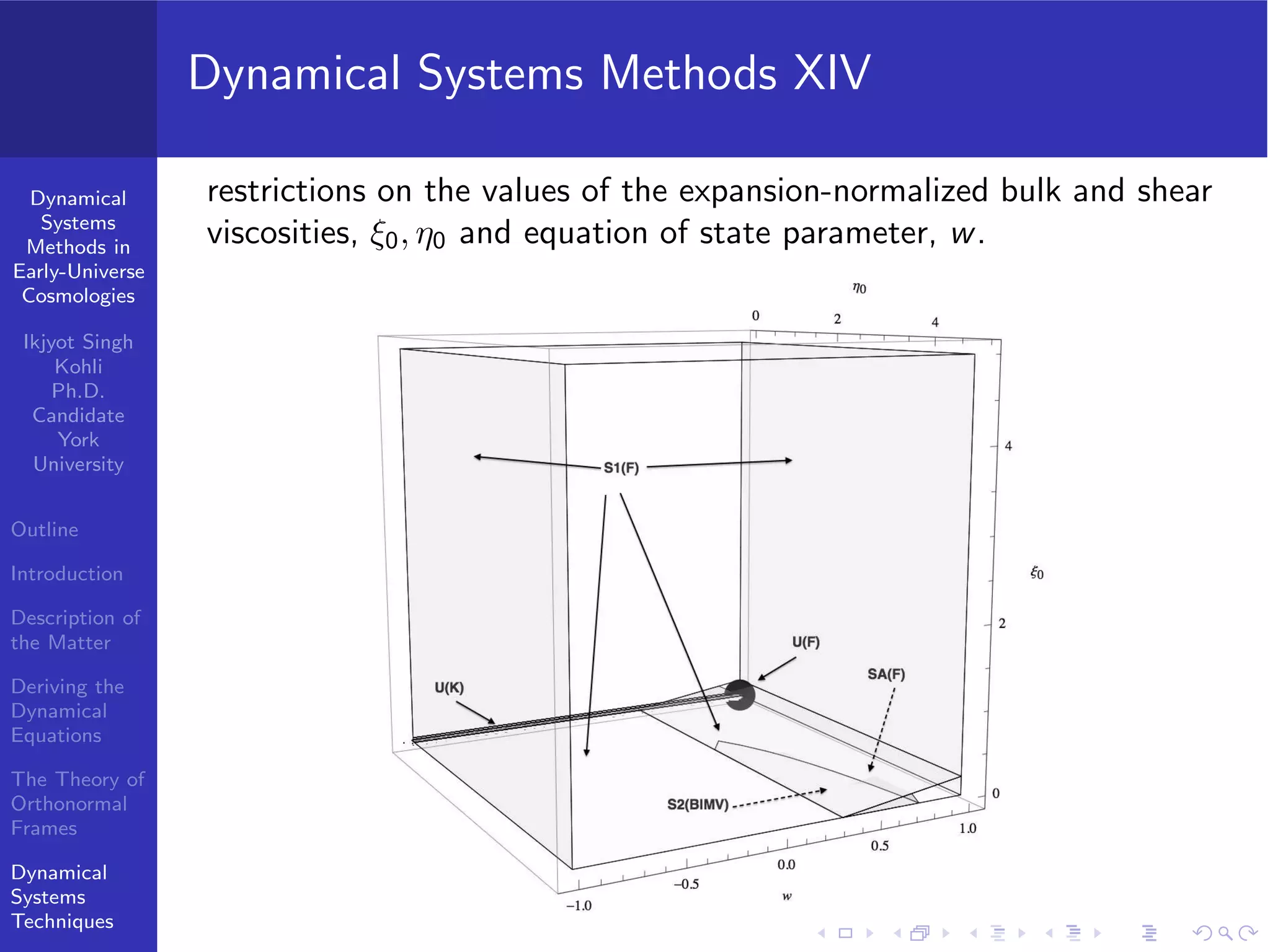
Describing solutions to Einstein field equations through dynamical systems and exploring effects of cosmological parameters.
Wrap-up on findings, significance of dynamical systems methods, and references for further insights into cosmological models.