This document discusses a context-aware recommender system using boolean matrix factorization, focusing on collaborative filtering and the use of contextual information in recommendations. It evaluates the effectiveness of the approach through quality metrics such as mean absolute error, precision, recall, and F-measure based on the MovieLens dataset. The authors highlight previous work in formal concept analysis and related areas, establishing a foundation for their proposed methodology.

1. Context-Aware Recommender System Based on
Boolean Matrix Factorisation
Marat Akhmatnurov and Dmitry I. Ignatov
National Research University Higher School of Economics, Moscow, Russia
Faculty of Computer Science
October 13–16, CLA 2015
Clermont-Ferrand, France

2. Outline
Problem Statement
Contextual information
Singular Value Decomposition
Related work
Boolean Matrix Factorisation
Quality evaluation
Conclusion and future work
Akhmatnurov & Ignatov Higher School of Economics CLA 2015 2 / 29

3. Recommender Systems
Collaborative Filtering
• Age
• Gender
• Occupation
• Location
• Genre
• Date
Akhmatnurov & Ignatov Higher School of Economics CLA 2015 3 / 29

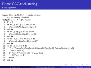
4. Contextual information
[Adomavicius & Tuzhilin, 2005]
I =
[
R Cuser
Citem O
]
,
Movies Sex Age
m1 m2 m3 m4 m5 m6 M F 0-20 21-45 46+
u1 5 5 5 2 + +
u2 5 5 3 5 + +
u3 4 4 5 4 + +
u4 3 5 5 5 + +
u5 2 5 4 + +
u6 5 3 4 5 + +
u7 5 4 5 4 + +
Drama + + + + +
Action + + + +
Comedy + +
Akhmatnurov & Ignatov Higher School of Economics CLA 2015 4 / 29

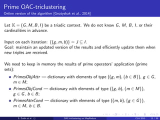
5. Singular Value Decomposition
SVD is de facto standard in RS domain [Koren et al., 2009]
Singular Value Decomposition (SVD) is a decomposition of a
rectangular matrix A ∈ Rm×n(m > n) into a product of three
matrices
A = U
(
Σ
0
)
VT
,
where U ∈ Rm×m and V ∈ Rn×n are orthogonal matrices, and
Σ ∈ Rn×n is a diagonal matrix such that Σ = diag(σ1, . . . , σn) and
σ1 ≥ σ2 ≥ . . . ≥ σn ≥ 0. The columns of the matrix U and V are
called singular vectors, and the numbers σi are singular values.
2mn2 + 2n3 floating-point operations [Trefthen et al., 1997]
Akhmatnurov & Ignatov Higher School of Economics CLA 2015 5 / 29

6. Related work
What about Formal Concept Analysis?
• du Boucher-Ryan et al., Collaborative recommending using
Formal Concept Analysis. Knowledge-Based Systems (2006)
• J¨aschke et al. Folksonomy (Bibsonomy) recommendations and
mining, since 2006
• Ignatov et al., Concept-based recommendations for internet
advertisement. CLA 2008
• Symeonidis et al., Nearest-biclusters collaborative filtering
based on constant and coherent values. Information Retrieval
(2008)
• Ignatov et al., Concept-Based Biclustering for Internet
Advertisement. IEEE ICDMW 2012
Akhmatnurov & Ignatov Higher School of Economics CLA 2015 6 / 29

7. Related work
What about Formal Concept Analysis?
• Jelassi et al., A personalized recommender system based on
users’ information in folksonomies. WWW 2013
• Alqadah et al., Biclustering neighborhood-based collaborative
filtering method for top-n recommender systems. Knowledge
and Information Systems (2014)
• Ignatov et al. Boolean Matrix Factorisation for Collaborative
Filtering: An FCA-Based Approach. AIMSA 2014 (FCA meets
IR @ ECIR 2013)
• Ignatov et al. RAPS: A recommender algorithm based on
pattern structures. FCA4AI@IJCAI 2015
Akhmatnurov & Ignatov Higher School of Economics CLA 2015 7 / 29

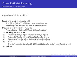
8. Boolean Matrix Factorisation
Formal Concept Analysis [Wille, 1982; Ganter & Wille, 1999]
A formal context K is a triple (G, M, I), where G is a set of
objects, M is a set of attributes, I ⊆ G × M is an incidence
relation. We write gIm when the object g ∈ G has the attribute
m ∈ M
Derivation (Galois) operators:
For A ⊆ G and for B ⊆ M we have
A′
= {m ∈ M | gIm for all g ∈ A} ,
B′
= {g ∈ G | gIm for all m ∈ B} .
A formal concept of the formal context K = (G, M, I) is a pair
(A, B) such that A ∈ G, B ∈ M, A′
= B and B′
= A.
Akhmatnurov & Ignatov Higher School of Economics CLA 2015 8 / 29

9. Boolean Matrix Factorisation
Formal Concept Analysis
B(G, M, I) is the set of all formal concepts of a context
K = (G, M, I).
F = {(A1, B1), . . . (Ak, Bk)} ⊆ B(G, M, I)
(PF )il =
{
1, i ∈ Al
0, otherwise
, l = 1, k,
(QF )lj =
{
1, j ∈ Bl
0, otherwise
, l = 1, k.
Akhmatnurov & Ignatov Higher School of Economics CLA 2015 9 / 29

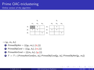
10. Boolean Matrix Factorisation
[Belohlavek & Vychodil, 2010]
Boolean matrix factorisation is a decomposition of the input binary
matrix I = {0, 1}m×n into a product of two binary matrices
P = {0, 1}m×k and Q = {0, 1}k×n by the following rule:
(P ◦ Q)ij =
k∨
l=1
Pil ∧ Qlj
Theorem 1 (Universality of formal concepts as factors)
For every binary matrix I there is F ⊆ B(G, M, I) such that
I = PF ◦ QF .
Theorem 2 (Optimality of formal concepts as factors)
Let I = P ◦ Q is a decomposition of I = {0, 1}m×n, where
P = {0, 1}m×k and Q = {0, 1}k×n. Then there exists
F ⊆ B(G, M, I) such that |F| ≤ k, I = PF ◦ QF .
Akhmatnurov & Ignatov Higher School of Economics CLA 2015 10 / 29

11. Boolean Matrix Factorisation
Searching for formal concept as factors
• Greedy algorithm (Belohlavek & Vychodil, 2010);
O(k|G||M|3), where k is the number of found factors.
• Close-by-one (CbO) algorithm (Kuznetsov S.O., 1993);
O(|G||M|2|L|)
• CbO modification with balanced factors (concepts)
W =
2|A||B|
|A|2 + |B|2
, where (A, B) ∈ B(G, M, I)
Akhmatnurov & Ignatov Higher School of Economics CLA 2015 11 / 29

12. Boolean Matrix Factorisation
• K = (U, M, I) is a user-to-movie rating formal context
m1 m2 m3 m4 m5 m6 f1 f2 f3 f4 f5
u1 1 0 1 1 0 0 0 1 1 0 0
u2 1 0 1 1 0 0 1 0 0 1 0
u3 1 0 1 1 0 1 0 1 0 1 0
u4 1 0 1 1 0 0 1 0 0 1 0
u5 0 0 0 0 1 1 1 0 0 0 1
u6 1 0 1 1 0 0 0 1 1 0 0
u7 1 0 0 1 1 1 1 0 0 0 1
g1 1 0 1 1 1 1 0 0 0 0 0
g2 0 1 1 0 1 1 0 0 0 0 0
g3 1 0 0 1 0 0 0 0 0 0 0
• ({u1, u3, u6, u7, g1, g2}, {m1, m4}),
• ({u2, u4}, {m2, m3, m6, f1, f4}),
• ({u5, u7}, {m5, m6, f1, f5}) ,
• ({u1, u6}, {m1, m3, m4, f2, f3}),
• ({u5, u7, g1, g3}, {m5, m6}),
• ({u2, u3, u4}, {m3, m6, f4}),
• ({u2, u4, g3}, {m2, m3, m6}),
• ({u1, u3, u6, g1}, {m1, m3, m4}),
• ({u1, u3, u6}, {m1, m3, m4, f2}).
Akhmatnurov & Ignatov Higher School of Economics CLA 2015 12 / 29

13. Boolean Matrix Factorisation
• 10 × 9 ◦ 9 × 12
















1 0 0 1 0 0 0 1 1
0 1 0 0 0 1 1 0 0
1 0 0 0 0 1 0 1 1
0 1 0 0 0 1 1 0 0
0 0 1 0 1 0 0 0 0
1 0 0 1 0 0 0 1 1
1 0 1 0 1 0 0 0 0
1 0 0 0 1 0 0 1 0
0 0 0 0 1 0 1 0 0
1 0 0 0 0 0 0 0 0
















◦














1 0 0 1 0 0 0 0 0 0 0
0 1 1 0 0 1 1 0 0 1 0
0 0 0 0 1 1 1 0 0 0 1
1 0 1 1 0 0 0 1 1 0 0
0 0 0 0 1 1 0 0 0 0 0
0 0 1 0 0 1 0 0 0 1 0
0 1 1 0 0 1 0 0 0 0 0
1 0 1 1 0 0 0 0 0 0 0
1 0 1 1 0 0 0 1 0 0 0














Akhmatnurov & Ignatov Higher School of Economics CLA 2015 13 / 29

14. Projections to the factor space
Boolean projection vs weighted projection
• ˜Puf =
∧
m∈u′
Ium · Qfm
• ˜Puf = (Iu· , Qf·)
||Qf·||1
=
∑
m∈M
Ium·Qfm
∑
m∈M
Qfm
















1 0 0 1 0 0 0 1 1
0 1 0 0 0 1 1 0 0
1 0 0 0 0 1 0 1 1
0 1 0 0 0 1 1 0 0
0 0 1 0 1 0 0 0 0
1 0 0 1 0 0 0 1 1
1 0 1 0 1 0 0 0 0
1 0 0 0 1 0 0 1 0
0 0 0 0 1 0 1 0 0
1 0 0 0 0 0 0 0 0
































1 1
5 0 1 0 1
3
1
3 1 1
0 1 1
2
1
5
1
2 1 1 1
3
1
4
1 3
5
1
4
4
5
1
2 1 2
3 1 1
0 1 1
2
1
5
1
2 1 1 1
3
1
4
0 2
5 1 0 1 2
3
1
3 0 0
1 1
5 0 1 0 1
3
1
3 1 1
1 2
5 1 1
5 1 1
3
1
3
2
3
1
2
1 2
5
1
2
2
5 1 2
3
2
3 1 3
4
0 2
5
1
2
1
5 1 2
3 1 1
3
1
4
1 0 0 1
5 0 0 0 2
3
1
2
















Akhmatnurov & Ignatov Higher School of Economics CLA 2015 14 / 29

15. User-based nearest neighbour approach
How to recommend?
• Similarity search
• simcos(u, v) = (ru , rv)
|ru|·|rv| =
∑
m∈M
rum·rim
√ ∑
m∈M
r2
um
√ ∑
m∈M
r2
vm
• simHam(u, v) = 1 −
∑
m∈M
|rum−rvm|
|M|
• Rating prediction
ˆrum =
∑
v∈ˆU
sim(v, u) · rvm
∑
v∈ˆU
sim(v, u)
,
Akhmatnurov & Ignatov Higher School of Economics CLA 2015 15 / 29

16. Quality evaluation of the proposed approach
Data
MovieLens-100k dataset
• 100 000 ratings (5-star scale)
• 943 users
• Gender
• Age
• Occupation (21 categories)
• ZIP
• 1682 movies
• 19 genres
Five star ratings are converted to binary scale:
Ium =
{
1, rum > 3,
0, else
Akhmatnurov & Ignatov Higher School of Economics CLA 2015 16 / 29

17. Quality evaluation
Criteria
• Mean Absolute Error
MAE =
∑
(u,m)∈U×M∩Itest
|ˆrum − rum|
|Itest|
• Precision
P =
TP
TP + FP
• Recall
R =
TP
TP + FN
• F-measure (F1-measure)
F =
2PR
P + R
Akhmatnurov & Ignatov Higher School of Economics CLA 2015 17 / 29

18. Quality evaluation
Bimodal cross-validation [Ignatov et al., 2012]
Akhmatnurov & Ignatov Higher School of Economics CLA 2015 18 / 29

19. Quality evaluation
Similarity measures
0 20 40 60 80 100
0.2
0.25
0.3
0.35
0.4
Number of neighbours
MAE
0 20 40 60 80 100
0.1
0.2
0.3
0.4
0.5
Number of neighbours
F−measure
0 20 40 60 80 100
0.2
0.4
0.6
0.8
1
Number of neighbours
Precision
0 20 40 60 80 100
0
0.1
0.2
0.3
0.4
Number of neighbours
Recall
Hamming
Cosine
Akhmatnurov & Ignatov Higher School of Economics CLA 2015 19 / 29

20. Quality evaluation
Projections
0 20 40 60 80 100
0.22
0.24
0.26
0.28
0.3
Number of neigbours
MAE
0 20 40 60 80 100
0
0.1
0.2
0.3
0.4
Number of neigbours
F−measure
0 20 40 60 80 100
0
0.2
0.4
0.6
0.8
Number of neigbours
Precision
0 20 40 60 80 100
0
0.1
0.2
0.3
0.4
Number of neigbours
Recall
Weighted projection
Boolean projection
Akhmatnurov & Ignatov Higher School of Economics CLA 2015 20 / 29

21. Quality evaluation
Number of covering factors
• BMF
p% =
|used marks|
|all marks|
100%
• SVD
p% =
K∑
i=1
σ2
i
∑
σ2
100%
Coverage 50% 60% 70% 80% 90%
Close-by-one 168 228 305 421 622
Belohlavek’s alg. 222 297 397 533 737
BMFCbO (no contextual information) 163 220 294 401 596
SVD 162 218 287 373 496
SVD (no contextual information) 157 211 277 361 480
Akhmatnurov & Ignatov Higher School of Economics CLA 2015 21 / 29

22. Quality evaluation
Coverage influence
Number
of
Precision Recall F-measure MAE
neighb. 60% 80% 60% 80% 60% 80% 60% 80%
1 0.3553 0.3609 0.2682 0.2647 0.3056 0.3054 0.2468 0.2434
5 0.6335 0.6442 0.1422 0.1412 0.2323 0.2317 0.2383 0.2359
10 0.7006 0.7045 0.1134 0.1114 0.1953 0.1924 0.2411 0.2388
15 0.7226 0.7258 0.0998 0.0979 0.1754 0.1726 0.2436 0.2411
20 0.7301 0.7373 0.0915 0.0903 0.1626 0.1610 0.2456 0.2429
25 0.7387 0.7427 0.0865 0.0853 0.1549 0.1531 0.2473 0.2445
30 0.7402 0.7426 0.0823 0.0818 0.1482 0.1474 0.2488 0.2459
40 0.7405 0.7508 0.0752 0.0759 0.1365 0.1379 0.2513 0.2484
50 0.7419 0.7487 0.0712 0.0712 0.1299 0.1301 0.2534 0.2504
60 0.7419 0.7478 0.0674 0.0678 0.1236 0.1243 0.2553 0.2522
70 0.7415 0.7477 0.0648 0.0654 0.1191 0.1202 0.2570 0.2538
80 0.7398 0.7449 0.0624 0.0624 0.1150 0.1151 0.2586 0.2553
100 0.7377 0.7461 0.0584 0.0583 0.1082 0.1081 0.2615 0.2580
Akhmatnurov & Ignatov Higher School of Economics CLA 2015 22 / 29

23. Quality evaluation
Algorithms for factor search
Number
of
Precision Recall F-measure MAE
neighb. Blhlv CbO Blhlv CbO Blhlv CbO Blhlv CbO
1 0.3626 0.3609 0.2582 0.2647 0.3016 0.3054 0.2436 0.2434
5 0.6435 0.6442 0.1331 0.1412 0.2205 0.2317 0.2371 0.2359
10 0.7127 0.7045 0.1061 0.1114 0.1848 0.1924 0.2395 0.2388
15 0.7323 0.7258 0.0936 0.0979 0.1660 0.1726 0.2415 0.2411
20 0.7424 0.7373 0.0860 0.0903 0.1542 0.1610 0.2429 0.2429
25 0.7479 0.7427 0.0812 0.0853 0.1465 0.1531 0.2442 0.2445
30 0.7519 0.7426 0.0774 0.0818 0.1403 0.1474 0.2454 0.2459
40 0.7579 0.7508 0.0721 0.0759 0.1317 0.1379 0.2475 0.2484
50 0.7569 0.7487 0.0678 0.0712 0.1244 0.1301 0.2492 0.2504
60 0.7602 0.7478 0.0651 0.0678 0.1199 0.1243 0.2507 0.2522
70 0.7600 0.7477 0.0623 0.0654 0.1151 0.1202 0.2520 0.2538
80 0.7589 0.7449 0.0601 0.0624 0.1114 0.1151 0.2531 0.2553
100 0.7559 0.7461 0.0562 0.0583 0.1046 0.1081 0.2553 0.2580
Akhmatnurov & Ignatov Higher School of Economics CLA 2015 23 / 29

24. Quality evaluation
Influence of contextual information (80% coverage)
Number Precision Recall F-measure MAE
of
neighb.
clean cntxt clean cntxt clean cntxt clean cntxt
1 0.3589 0.3609 0.2668 0.2647 0.3061 0.3054 0.2446 0.2434
5 0.6353 0.6442 0.1420 0.1412 0.2321 0.2317 0.2371 0.2359
10 0.6975 0.7045 0.1126 0.1114 0.1938 0.1924 0.2399 0.2388
15 0.7168 0.7258 0.0994 0.0979 0.1746 0.1726 0.2422 0.2411
20 0.7282 0.7373 0.0911 0.0903 0.1619 0.1610 0.2442 0.2429
25 0.7291 0.7427 0.0861 0.0853 0.1540 0.1531 0.2457 0.2445
30 0.7318 0.7426 0.0823 0.0818 0.1480 0.1474 0.2472 0.2459
40 0.7342 0.7508 0.0767 0.0759 0.1389 0.1379 0.2497 0.2484
50 0.7332 0.7487 0.0716 0.0712 0.1304 0.1301 0.2518 0.2504
60 0.7314 0.7478 0.0682 0.0678 0.1247 0.1243 0.2536 0.2522
70 0.7333 0.7477 0.0658 0.0654 0.1208 0.1202 0.2552 0.2538
80 0.7342 0.7449 0.0632 0.0624 0.1164 0.1151 0.2567 0.2553
100 0.7299 0.7461 0.0590 0.0583 0.1092 0.1081 0.2594 0.2580
Akhmatnurov & Ignatov Higher School of Economics CLA 2015 24 / 29

25. Quality evaluation
Comparison with SVD
0 20 40 60 80 100
0.2
0.25
0.3
0.35
0.4
Number of neighbours
MAE
0 20 40 60 80 100
0
0.1
0.2
0.3
0.4
Number of neighbours
F−measure
0 20 40 60 80 100
0.2
0.4
0.6
0.8
1
Number of neighbours
Precision
0 20 40 60 80 100
0
0.1
0.2
0.3
0.4
Number of neighbours
Recall
BMF80
+context
SVD85
+context
SVD85
Akhmatnurov & Ignatov Higher School of Economics CLA 2015 25 / 29

26. Conclusion
• We have proposed a rather straightforward BMF-based
approach for recommendations with contextual information
• MAE of our BMF-based approach is sufficiently lower than
MAE of SVD-based approach for almost the same number of
factors at fixed coverage level.
• The Precision of BMF-based approach is slightly lower when
the number of neighbours is about a couple of dozens and
comparable for the remaining observed range.
• The Recall is lower that results in lower F-measure.
Akhmatnurov & Ignatov Higher School of Economics CLA 2015 26 / 29

27. Conclusion
• The greedy algorithm of Belohlavek & Vychodyl results in
more factors with larger extent, but it is faster and shows
almost the same quality as the balanced factors search by
CbO.
• Our weighted projection alleviates the information loss of
Boolean projection and results in a substantial quality gain.
• Contextual information demonstrates a small quality increase
(about 1-2%) in terms of MAE and Precision, but not in
Recall and Precision.
Akhmatnurov & Ignatov Higher School of Economics CLA 2015 27 / 29

28. Future work
• Incorporation of time and location as contextual information
• Treatment of contextual information by means of Triadic FCA
and triclustering
• Comparison, usage, extension of the following works:
• [Jelassi et al., 2013] Recommendations in personalised
folksomies
• [Belohlávek et al, 2013] Factorization of three-way binary data
using triadic concepts
• [Trnecka et al., 2014] Multi-Relational Boolean Factor
Analysis
• [Belholavek et al., 2015; Metzler et al., 2015; Nourine et. al.,
2015] Efficient Boolean matrix factorisation algorithms
Akhmatnurov & Ignatov Higher School of Economics CLA 2015 28 / 29

29. Thank you!
Questions?
Akhmatnurov & Ignatov Higher School of Economics CLA 2015 29 / 29