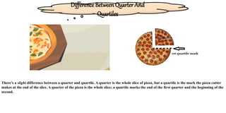
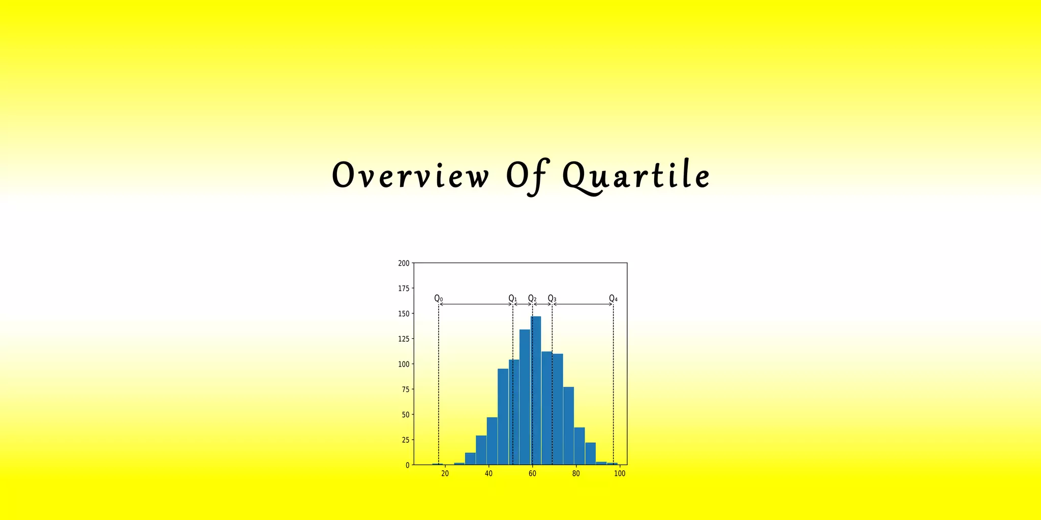
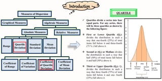
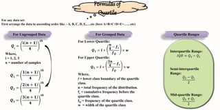
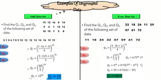
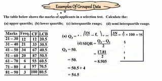
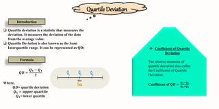
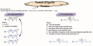
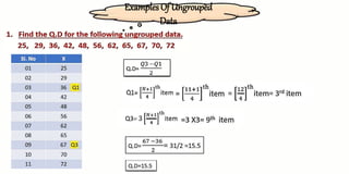
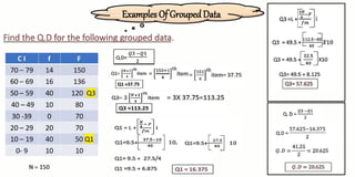
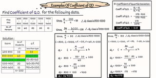
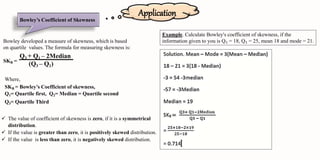
Overview Of Quartile
Introduction
Measures of Dispersion
Algebraic Measures
Graphical Measures
Absolute Measures Relative Measures
Range
Quartile
Deviation
Standard
Deviation
Mean
Deviation
Coefficient
of Range
Coefficient
of Variation
Coefficient
of Quartile
Deviation
Coefficient
of Mean
Deviation
 Quartiles divide a series into four
equal parts. For any series, there
will be three quartiles as shown by
the following figure:
 First or Lower Quartile (Q1):
divides the distribution in such a
way that one-fourth (25%) of total
items fall below it and three-fourth
(75 % ) fall above it.
 Second or (Q2) or Median: divides
the distribution in such a way that
half (50%) of total items fall below
it and half (50%) above it.
 Third or Upper Quartile (Q3): Q3
divides the distribution in such a
way that three fourth (75%) of total
items fall below it and one- fourth
(25%) fall above it.
QUARTILE
Formulas of
Quartile
For Ungrouped Data For Grouped Data
For any data set:
First arrange the data in ascending order like – A, B, C, D, E,….etc (here A>B>C>D>E>……etc)
𝑸ⅈ
=
ⅈ 𝒏 + 𝟏
𝟒
𝒕𝒉
Where,
i = 1, 2, 3
n = number of samples
𝑸𝟑 =
𝟑 𝒏 + 𝟏
𝟒
𝒕𝒉
𝑸𝟐 =
𝟐 𝒏 + 𝟏
𝟒
𝒕𝒉
𝑸𝟏 =
𝟏 𝒏 + 𝟏
𝟒
𝒕𝒉
For Lower Quartile:
𝑸𝟏 = 𝒍 +
𝒏
𝟒
− 𝒇𝒄
𝒇𝑸
× 𝒘
For Upper Quartile:
𝑸𝟑 = 𝒍 +
𝟑𝒏
𝟒
− 𝒇𝒄
𝒇𝑸
× 𝒘
Where,
l = lower class boundary of the quartile
class.
n = total frequency of the distribution.
fc = cumulative frequency before the
quartile class.
fQ = frequency of the quartile class.
w = width of the quartile class
Quartile Ranges
Interquartile Range:
𝐼𝑄𝑅 = 𝑄3 − 𝑄1
Semi-interquartile
Range:
𝑄3 − 𝑄1
2
Mid-quartile Range:
𝑄3 + 𝑄1
2
Examples Of Ungrouped
Data
Odd Data Set Even Data Set
Q1
Q2
Q3
Q1
Q2
Q3
Examples Of GroupedData
Quartile Deviation
Introduction
 Quartile deviation is a statistic that measures the
deviation. It measures the deviation of the data
from the average value.
 Quartile Deviation is also known as the Semi
Interquartile range. It can be represented as QD;
Formula
𝑸𝑫 =
𝑸𝟑 − 𝑸𝟏
𝟐
Where,
𝑸𝑫= quartile deviation
𝑸𝟑 = 𝐮𝐩𝐩𝐞𝐫 𝐪𝐮𝐚𝐫𝐭ⅈ𝐥𝐞
𝑸𝟏= lower quartile
 Coefficient of Quartile
Deviation
The relative measures of
quartile deviation also called
the Coefficient of Quartile
Deviation.
Coefficient of 𝑸𝑫 =
𝑸𝟑−𝑸𝟏
𝑸𝟑+𝑸𝟏
Formula Of Quartile
Deviation
For Ungrouped Data
For any data set:
First arrange the data in ascending order like – A, B, C, D, E,….etc (here A>B>C>D>E>……etc)
𝑸ⅈ
=
ⅈ 𝒏 + 𝟏
𝟒
𝒕𝒉
Where,
i = 1, 2, 3
n = number of samples
𝑸𝟑 =
𝟑 𝒏 + 𝟏
𝟒
𝒕𝒉
𝑸𝟐 =
𝟐 𝒏 + 𝟏
𝟒
𝒕𝒉
𝑸𝟏 =
𝟏 𝒏 + 𝟏
𝟒
𝒕𝒉
For Grouped Data
𝑸𝐫 = 𝒍𝟏 +
𝒓
𝑵
𝟒
− 𝑪
𝒇
𝒍𝟐 − 𝒍𝟏
Where,
Qr = the rth quartile
l1 = the lower limit of the quartile class
l2 = the upper limit of the quartile class
f = the frequency of the quartile class
c = the cumulative frequency of the class preceding the quartile class
N = Number of observations in the given data set
𝑸𝟏 = 𝒍𝟏 +
𝟏
𝑵
𝟒
− 𝑪
𝒇
𝒍𝟐 − 𝒍𝟏 𝑸𝟑 = 𝒍𝟏 +
𝟑
𝑵
𝟒
− 𝑪
𝒇
𝒍𝟐 − 𝒍𝟏
Examples Of Ungrouped
Data
Examples Of GroupedData
Examples Of Coefficient of QD
Application
Bowley’s Coefficient of Skewness
Bowley developed a measure of skewness, which is based
on quartile values. The formula for measuring skewness is:
SKB =
Q3 + Q1 – 2Median
(Q3 – Q1)
Where,
SKB = Bowley’s Coefficient of skewness,
Q1= Quartile first, Q2= Median = Quartile second
Q3= Quartile Third
 The value of coefficient of skewness is zero, if it is a symmetrical
distribution.
 If the value is greater than zero, it is positively skewed distribution.
 If the value is less than zero, it is negatively skewed distribution.
Example. Calculate Bowley's coefficient of skewness, if the
information given to you is Q₁ = 18, Q₁ = 25, mean 18 and mode = 21.
Application
D A T A S E T
Box And Whisker Plot
A box and whisker plot is defined as a graphical method of displaying variation in a set of
data. In most cases, a histogram analysis provides a sufficient display, but a box and
whisker plot can provide additional detail while allowing multiple sets of data to be
displayed in the same graph.
from statistics import*
example_list = (24,28,31,35,36,37,39,41,44)
print("data set =",example_list)
Q2=median(example_list)
print("Q2 =",Q2)
small_set=example_list[0:4]
large_set=example_list[5:9]
print(“lower set -", small_set)
print(" Upper set -", large_set)
Q1=median(small_set)
Q3=median(large_set)
print("Q1 =",Q1)
print("Q3 =",Q3)
quatile_deviation=(Q3-Q1)/2
print("Quartile deviation =",quatile_deviation)
coefficient_of_QD=(Q3-Q1)/(Q3+Q1)
print("coefficient of quartile deviation =",coefficient_of_QD)
data set = (24, 28, 31, 35, 36, 37, 39, 41, 44)
Q2 = 36
lower set - (24, 28, 31, 35)
Upper set - (37, 39, 41, 44)
Q1 = 29.5
Q3 = 40.0
Quartile deviation = 5.25
coefficient of quartile deviation = 0.1510791366906475
RUN
Quartile And Quartile Deviation Via
Python
import numpy
x = [17,10,9,14,13,17,12,20,14]
print ("A :",x)
Q1 = numpy.quantile (x, .25)
Q2 = numpy.quantile (x, .50)
Q3 = numpy.quantile (x, .75)
print("Q1 :",Q1)
print("Q2 :",Q2)
print("Q3 :",Q3)
Interquartilerange = Q3-Q1
Quartiledeviation = Interquartilerange/2
print("Q.D :",Quartiledeviation)
A : [17, 10, 9, 14, 13, 17, 12, 20, 14]
Q1 : 12.0
Q2 : 14.0
Q3 : 17.0
Q.D : 2.5
RUN
Quartile And Quartile Deviation Via
Python
scores<- c(78, 93, 68, 84, 90, 74, 64, 55, 80)
scores
sort(scores)
min(scores)
max(scores)
median(scores)
quantile(scores)
quantile(scores, 0.25)
quantile(scores, 0.75)
quantile(scores, c(0.25, 0.5, 0.75))
fivenum(scores)
summary(scores)
par(mfrow = c(1, 2))
boxplot(scores)
boxplot(scores)
abline(h = min(scores), col = "Blue")
abline(h = max(scores), col = "Yellow")
abline(h = median(scores), col = "Green")
abline(h = quantile(scores, c(0.25, 0.75)), col = "Red")
> scores<- c(78, 93, 68, 84, 90, 74, 64, 55, 80)
> scores
[1] 78 93 68 84 90 74 64 55 80
> sort(scores)
[1] 55 64 68 74 78 80 84 90 93
> min(scores)
[1] 55
> max(scores)
[1] 93
> median(scores)
[1] 78
> quantile(scores)
0% 25% 50% 75% 100%
55 68 78 84 93
> quantile(scores, 0.25)
25%
68
> quantile(scores, 0.75)
75%
84
> quantile(scores, c(0.25, 0.5, 0.75))
25% 50% 75%
68 78 84
> fivenum(scores)
[1] 55 68 78 84 93
> summary(scores)
Min. 1st Qu. Median Mean 3rd Qu. Max.
55.00 68.00 78.00 76.22 84.00 93.00
> par(mfrow = c(1, 2))
> boxplot(scores)
> boxplot(scores)
> abline(h = min(scores), col = "Blue")
> abline(h = max(scores), col = "Yellow")
> abline(h = median(scores), col = "Green")
> abline(h = quantile(scores, c(0.25, 0.75)), col = "Red")
RUN
QuartileAnd Boxand
whisker plots Via R code
Difference Between Quarter And
Quartiles
There’s a slight difference between a quarter and quartile. A quarter is the whole slice of pizza, but a quartile is the mark the pizza cutter
makes at the end of the slice. A quarter of the pizza is the whole slice; a quartile marks the end of the first quarter and the beginning of the
second.
THANK YOU

Overview Of Quartile.pptx

  • 1.
  • 2.
    Introduction Measures of Dispersion AlgebraicMeasures Graphical Measures Absolute Measures Relative Measures Range Quartile Deviation Standard Deviation Mean Deviation Coefficient of Range Coefficient of Variation Coefficient of Quartile Deviation Coefficient of Mean Deviation  Quartiles divide a series into four equal parts. For any series, there will be three quartiles as shown by the following figure:  First or Lower Quartile (Q1): divides the distribution in such a way that one-fourth (25%) of total items fall below it and three-fourth (75 % ) fall above it.  Second or (Q2) or Median: divides the distribution in such a way that half (50%) of total items fall below it and half (50%) above it.  Third or Upper Quartile (Q3): Q3 divides the distribution in such a way that three fourth (75%) of total items fall below it and one- fourth (25%) fall above it. QUARTILE
  • 3.
    Formulas of Quartile For UngroupedData For Grouped Data For any data set: First arrange the data in ascending order like – A, B, C, D, E,….etc (here A>B>C>D>E>……etc) 𝑸ⅈ = ⅈ 𝒏 + 𝟏 𝟒 𝒕𝒉 Where, i = 1, 2, 3 n = number of samples 𝑸𝟑 = 𝟑 𝒏 + 𝟏 𝟒 𝒕𝒉 𝑸𝟐 = 𝟐 𝒏 + 𝟏 𝟒 𝒕𝒉 𝑸𝟏 = 𝟏 𝒏 + 𝟏 𝟒 𝒕𝒉 For Lower Quartile: 𝑸𝟏 = 𝒍 + 𝒏 𝟒 − 𝒇𝒄 𝒇𝑸 × 𝒘 For Upper Quartile: 𝑸𝟑 = 𝒍 + 𝟑𝒏 𝟒 − 𝒇𝒄 𝒇𝑸 × 𝒘 Where, l = lower class boundary of the quartile class. n = total frequency of the distribution. fc = cumulative frequency before the quartile class. fQ = frequency of the quartile class. w = width of the quartile class Quartile Ranges Interquartile Range: 𝐼𝑄𝑅 = 𝑄3 − 𝑄1 Semi-interquartile Range: 𝑄3 − 𝑄1 2 Mid-quartile Range: 𝑄3 + 𝑄1 2
  • 4.
    Examples Of Ungrouped Data OddData Set Even Data Set Q1 Q2 Q3 Q1 Q2 Q3
  • 5.
  • 6.
    Quartile Deviation Introduction  Quartiledeviation is a statistic that measures the deviation. It measures the deviation of the data from the average value.  Quartile Deviation is also known as the Semi Interquartile range. It can be represented as QD; Formula 𝑸𝑫 = 𝑸𝟑 − 𝑸𝟏 𝟐 Where, 𝑸𝑫= quartile deviation 𝑸𝟑 = 𝐮𝐩𝐩𝐞𝐫 𝐪𝐮𝐚𝐫𝐭ⅈ𝐥𝐞 𝑸𝟏= lower quartile  Coefficient of Quartile Deviation The relative measures of quartile deviation also called the Coefficient of Quartile Deviation. Coefficient of 𝑸𝑫 = 𝑸𝟑−𝑸𝟏 𝑸𝟑+𝑸𝟏
  • 7.
    Formula Of Quartile Deviation ForUngrouped Data For any data set: First arrange the data in ascending order like – A, B, C, D, E,….etc (here A>B>C>D>E>……etc) 𝑸ⅈ = ⅈ 𝒏 + 𝟏 𝟒 𝒕𝒉 Where, i = 1, 2, 3 n = number of samples 𝑸𝟑 = 𝟑 𝒏 + 𝟏 𝟒 𝒕𝒉 𝑸𝟐 = 𝟐 𝒏 + 𝟏 𝟒 𝒕𝒉 𝑸𝟏 = 𝟏 𝒏 + 𝟏 𝟒 𝒕𝒉 For Grouped Data 𝑸𝐫 = 𝒍𝟏 + 𝒓 𝑵 𝟒 − 𝑪 𝒇 𝒍𝟐 − 𝒍𝟏 Where, Qr = the rth quartile l1 = the lower limit of the quartile class l2 = the upper limit of the quartile class f = the frequency of the quartile class c = the cumulative frequency of the class preceding the quartile class N = Number of observations in the given data set 𝑸𝟏 = 𝒍𝟏 + 𝟏 𝑵 𝟒 − 𝑪 𝒇 𝒍𝟐 − 𝒍𝟏 𝑸𝟑 = 𝒍𝟏 + 𝟑 𝑵 𝟒 − 𝑪 𝒇 𝒍𝟐 − 𝒍𝟏
  • 8.
  • 9.
  • 10.
  • 11.
    Application Bowley’s Coefficient ofSkewness Bowley developed a measure of skewness, which is based on quartile values. The formula for measuring skewness is: SKB = Q3 + Q1 – 2Median (Q3 – Q1) Where, SKB = Bowley’s Coefficient of skewness, Q1= Quartile first, Q2= Median = Quartile second Q3= Quartile Third  The value of coefficient of skewness is zero, if it is a symmetrical distribution.  If the value is greater than zero, it is positively skewed distribution.  If the value is less than zero, it is negatively skewed distribution. Example. Calculate Bowley's coefficient of skewness, if the information given to you is Q₁ = 18, Q₁ = 25, mean 18 and mode = 21.
  • 12.
    Application D A TA S E T Box And Whisker Plot A box and whisker plot is defined as a graphical method of displaying variation in a set of data. In most cases, a histogram analysis provides a sufficient display, but a box and whisker plot can provide additional detail while allowing multiple sets of data to be displayed in the same graph.
  • 13.
    from statistics import* example_list= (24,28,31,35,36,37,39,41,44) print("data set =",example_list) Q2=median(example_list) print("Q2 =",Q2) small_set=example_list[0:4] large_set=example_list[5:9] print(“lower set -", small_set) print(" Upper set -", large_set) Q1=median(small_set) Q3=median(large_set) print("Q1 =",Q1) print("Q3 =",Q3) quatile_deviation=(Q3-Q1)/2 print("Quartile deviation =",quatile_deviation) coefficient_of_QD=(Q3-Q1)/(Q3+Q1) print("coefficient of quartile deviation =",coefficient_of_QD) data set = (24, 28, 31, 35, 36, 37, 39, 41, 44) Q2 = 36 lower set - (24, 28, 31, 35) Upper set - (37, 39, 41, 44) Q1 = 29.5 Q3 = 40.0 Quartile deviation = 5.25 coefficient of quartile deviation = 0.1510791366906475 RUN Quartile And Quartile Deviation Via Python
  • 14.
    import numpy x =[17,10,9,14,13,17,12,20,14] print ("A :",x) Q1 = numpy.quantile (x, .25) Q2 = numpy.quantile (x, .50) Q3 = numpy.quantile (x, .75) print("Q1 :",Q1) print("Q2 :",Q2) print("Q3 :",Q3) Interquartilerange = Q3-Q1 Quartiledeviation = Interquartilerange/2 print("Q.D :",Quartiledeviation) A : [17, 10, 9, 14, 13, 17, 12, 20, 14] Q1 : 12.0 Q2 : 14.0 Q3 : 17.0 Q.D : 2.5 RUN Quartile And Quartile Deviation Via Python
  • 15.
    scores<- c(78, 93,68, 84, 90, 74, 64, 55, 80) scores sort(scores) min(scores) max(scores) median(scores) quantile(scores) quantile(scores, 0.25) quantile(scores, 0.75) quantile(scores, c(0.25, 0.5, 0.75)) fivenum(scores) summary(scores) par(mfrow = c(1, 2)) boxplot(scores) boxplot(scores) abline(h = min(scores), col = "Blue") abline(h = max(scores), col = "Yellow") abline(h = median(scores), col = "Green") abline(h = quantile(scores, c(0.25, 0.75)), col = "Red") > scores<- c(78, 93, 68, 84, 90, 74, 64, 55, 80) > scores [1] 78 93 68 84 90 74 64 55 80 > sort(scores) [1] 55 64 68 74 78 80 84 90 93 > min(scores) [1] 55 > max(scores) [1] 93 > median(scores) [1] 78 > quantile(scores) 0% 25% 50% 75% 100% 55 68 78 84 93 > quantile(scores, 0.25) 25% 68 > quantile(scores, 0.75) 75% 84 > quantile(scores, c(0.25, 0.5, 0.75)) 25% 50% 75% 68 78 84 > fivenum(scores) [1] 55 68 78 84 93 > summary(scores) Min. 1st Qu. Median Mean 3rd Qu. Max. 55.00 68.00 78.00 76.22 84.00 93.00 > par(mfrow = c(1, 2)) > boxplot(scores) > boxplot(scores) > abline(h = min(scores), col = "Blue") > abline(h = max(scores), col = "Yellow") > abline(h = median(scores), col = "Green") > abline(h = quantile(scores, c(0.25, 0.75)), col = "Red") RUN QuartileAnd Boxand whisker plots Via R code
  • 16.
    Difference Between QuarterAnd Quartiles There’s a slight difference between a quarter and quartile. A quarter is the whole slice of pizza, but a quartile is the mark the pizza cutter makes at the end of the slice. A quarter of the pizza is the whole slice; a quartile marks the end of the first quarter and the beginning of the second.
  • 17.