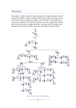
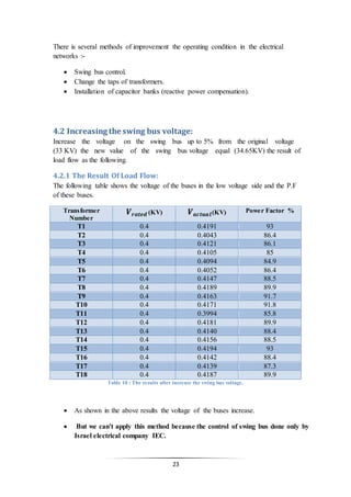
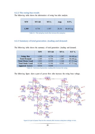
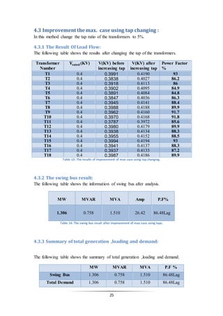
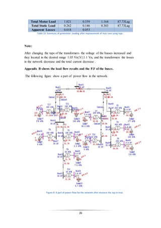
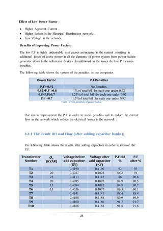
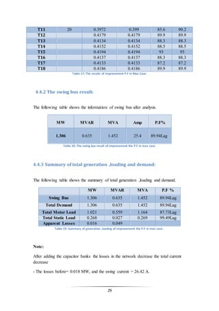
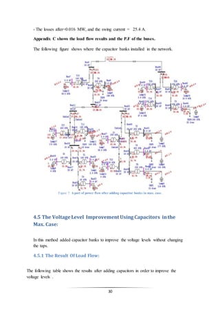
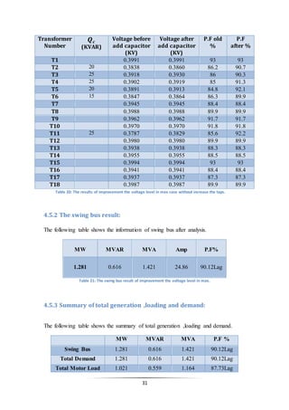
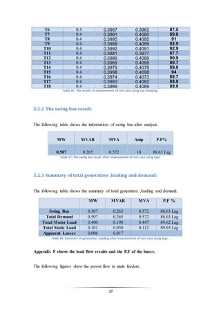
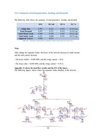
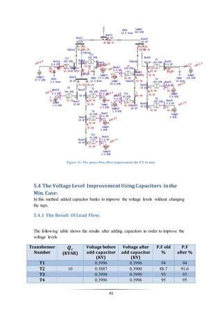
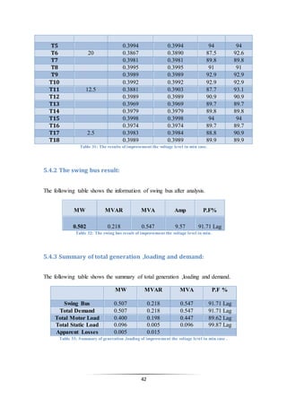
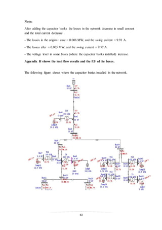
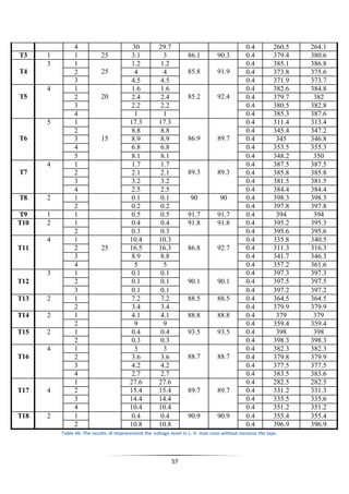
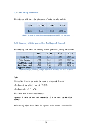
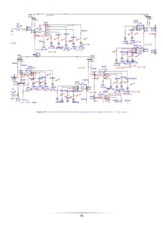
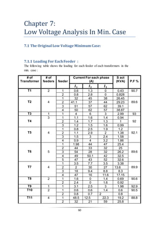
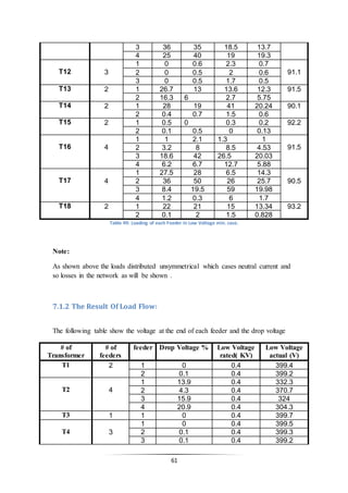
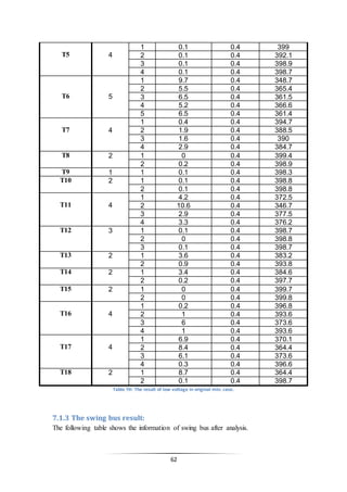
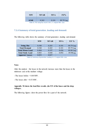
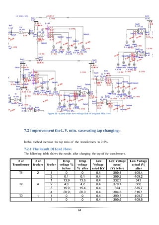
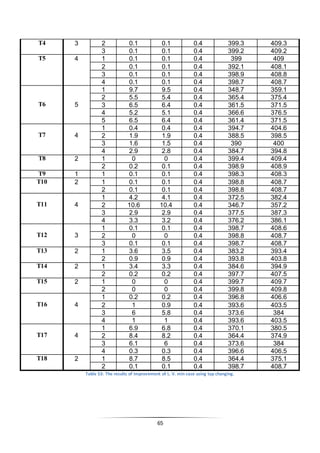
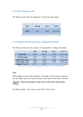
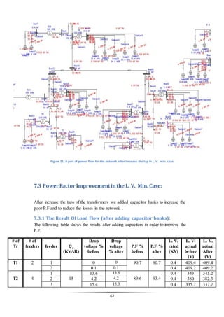
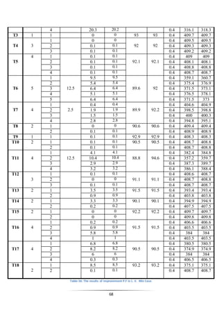
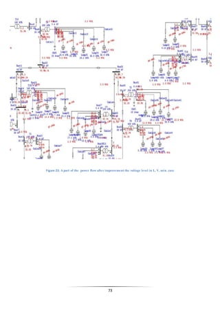
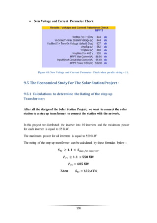
0
1
Contents
Contents ......................................................................................................................................... 0
Index of Figures............................................................................................................................ 5
Index of Tables............................................................................................................................ 7
Abstract ......................................................................................................................................... 9
Chapter 1 : Introduction
1.1 Electrical Power System: ...................................................................................................... 10
1.2 Load Flow Study:............................................................................................................... 10
1.3 ETAP power station 7 :...................................................................................................... 11
1.4 About Our Project :............................................................................................................ 12
Chapter 2 : Information about Aqraba Network
2.1 Elements Of Network: .......................................................................................................... 14
2.1.1 Electrical Supply: ............................................................................................................ 14
2.1.2 Distribution Transformers:........................................................................................... 14
2.1.3 Over Head Line:............................................................................................................... 16
2.1.4 Under Ground Cable : ...................................................................................................... 17
Chapter 3 : Load Flow Analysis
3.1 Transformer Loading (At Max. Case ) : ................................................................................. 18
Chapter 4 : Maximum Case Improvement
4.1 The Original Maximum Case: ............................................................................................... 20
4.1.1 The Result Of Load Flow:................................................................................................ 20
4.1.2 The swing bus result:........................................................................................................ 20
4.1.3 Summary of total generation ,loading and demand: ........................................................ 21
4.2 Increasing the swing bus voltage:........................................................................................... 23
4.2.1 The Result Of Load Flow:................................................................................................ 23
4.2.2 The swing bus result:........................................................................................................ 24
4.2.3 Summary of total generation ,loading and demand: ........................................................ 24
4.3 Improvement the max. case using tap changing :.................................................................. 25
4.3.1 The Result Of Load Flow:................................................................................................ 25
4.3.2 The swing bus result:........................................................................................................ 25
4.3.3 Summary of total generation ,loading and demand: ........................................................ 25
2
4.4 Power Factor Improvement in the Max. Case: ....................................................................... 27
4.4.1 The Result Of Load Flow:................................................................................................ 28
4.4.2 The swing bus result:........................................................................................................ 29
4.3.3 Summary of total generation ,loading and demand: ........................................................ 29
4.5 The Voltage Level Improvement Using Capacitors in the Max. Case: ................................ 30
4.5.1 The Result Of Load Flow:................................................................................................ 31
4.5.2 The swing bus result:........................................................................................................ 31
4.5.3 Summary of total generation ,loading and demand: ........................................................ 31
Chapter 5 : Minimum Case Improvement
5.1 The Original Minimum Case: ................................................................................................. 33
5.1.1 Transformer Loading : .................................................................................................... 33
5.1.2 The Result Of Load Flow:................................................................................................ 34
5.1.3 The swing bus result:........................................................................................................ 34
5.1.4 Summary of total generation ,loading and demand: ........................................................ 34
5.2 Improvement the minimum case using tap changing : ........................................................... 36
5.2.1 The Result Of Load Flow:................................................................................................ 37
5.2.2 The swing bus result:........................................................................................................ 37
5.2.3 Summary of total generation ,loading and demand: ........................................................ 37
5.3 Power Factor Improvement in the Min. Case:........................................................................ 39
5.3.1 The Result Of Load Flow:................................................................................................ 39
5.3.2 The swing bus result:........................................................................................................ 39
5.3.3 Summary of total generation ,loading and demand: ........................................................ 40
5.4 The Voltage Level Improvement Using Capacitors in the Min. Case:................................. 41
5.4.1 The Result Of Load Flow:................................................................................................ 41
5.4.2 The swing bus result:........................................................................................................ 42
5.4.3 Summary of total generation ,loading and demand: ........................................................ 42
Chapter 6 : Low Voltage Analysis In Max. Case
6.1 Low Voltage Side: .................................................................................................................. 45
6.2 The Original Low Voltage Max. Case :.................................................................................. 45
6.2.1 Loading For Each Feeder:................................................................................................ 46
6.2.2 The Result Of Load Flow:................................................................................................ 47
6.2.3 The swing bus result:........................................................................................................ 48
3
6.2.4 Summary of total generation ,loading and demand: ........................................................ 48
6.3 Improvement The Low Voltage Max. Case Using Tap Changing: ........................................ 50
6.3.1 The Result Of Load Flow:................................................................................................ 51
6.3.2 The swing bus result:........................................................................................................ 52
6.3.3 Summary of total generation ,loading and demand: ........................................................ 52
6.4 Power Factor Improvement in the Low Voltage Max. Case: ................................................. 53
6.4.1 The Result Of Load Flow:................................................................................................ 53
6.4.2 The swing bus result:........................................................................................................ 55
6.4.3 Summary of total generation ,loading and demand: ........................................................ 55
6.5 The Voltage Level Improvement Using Capacitors in Low Voltage Max. Case:................ 56
6.5.1 The Result Of Load Flow:................................................................................................ 56
6.5.2 The swing bus result:........................................................................................................ 58
6.5.3 Summary of total generation ,loading and demand: ........................................................ 58
Chapter 7 : Low Voltage Analysis In Min. Case
7.1 The Original Low Voltage Min. Case : .................................................................................. 60
7.1.1 Loading For Each Feeder:................................................................................................ 60
7.1.2 The Result Of Load Flow:................................................................................................ 61
7.1.3 The swing bus result:........................................................................................................ 62
7.1.4 Summary of total generation ,loading and demand: ........................................................ 63
7.2 Improvement The Low Voltage Min. Case Using Tap Changing:......................................... 64
7.2.1 The Result Of Load Flow:................................................................................................ 64
7.2.2 The swing bus result:........................................................................................................ 66
7.2.3 Summary of total generation ,loading and demand: ........................................................ 66
7.3 Power Factor Improvement in the Low Voltage Min. Case:.................................................. 67
7.3.1 The Result Of Load Flow:................................................................................................ 67
7.3.2 The swing bus result:........................................................................................................ 69
7.3.3 Summary of total generation ,loading and demand: ........................................................ 69
7.4 The Voltage Level Improvement Using Capacitors in Low Voltage Min. Case:................. 70
7.4.1 The Result Of Load Flow:................................................................................................ 70
7.4.2 The swing bus result:........................................................................................................ 72
7.4.3 Summary of total generation ,loading and demand: ........................................................ 72
4
Chapter 8 : The Economical Study
8.1 Saving In Panelties :............................................................................................................... 74
8.2 Saving In Losses : .................................................................................................................. 75
8.3 Simple Pay Back Period : ....................................................................................................... 75
Chapter 9 : Solar Energy Station Project
9.1 Solar System: .......................................................................................................................... 76
9.1.1 Introduction to Solar System:........................................................................................... 76
9.1.2 Solar Building Designs: ................................................................................................... 77
9.1.3 Solar Photovoltaic Energy:............................................................................................... 78
9.2 Consumption Energy Of Network and Solar System Design:................................................ 79
9.2.1 Data about Energy Consumption of the Network:........................................................... 79
9.2.2 Calculations of the power for the Solar System:.............................................................. 80
9.2.3 The Optimization tilt angle Tracking system:.................................................................. 80
9.3 The Design of the solar station system: ................................................................................. 87
9.3.1 Design Of Solar System PV system:................................................................................ 88
9.3.2 Calculations For the Fixed Cost of the investment by PV system:.................................. 92
9.4 The Design of the solar station system by using Power One (Aurora):................................. 95
9.5 The Economical Study For The Solar Station Project:......................................................... 100
9.5.1 Calculations to determine the Rating of the step up Transformer: ................................ 100
9.5.2 Economical Study for the Solar system Project:............................................................ 101
Chapter 10 : Sag & Tension In Overhead Lines Problem
10.1 Sag In Overhead Lines........................................................................................................ 102
10.1.1 Introduction:................................................................................................................. 102
10.1.1 Calculations Of Sag:..................................................................................................... 103
10.2 Problem of the Sag in Overhead Lines in the Network: ..................................................... 104
10.3 Solutions and Recommendations for Sag problem:........................................................... 105
References :............................................................................................................................. 106
5
Index of Figures
Figure 1: One Line Diagram Of Aqraba Network..................................................................................9
Figure 2: ETAP power station 7.........................................................................................................11
Figure 3: Figure Of Transformer........................................................................................................14
Figure 4: ACSR Cable. .....................................................................................................................16
Figure 5:XLPE Cable........................................................................................................................17
Figure 6: The power flow for the network in the original max case.......................................................22
Figure 7: A part of power flow for the network after increase swing buse voltage in max.. ....................24
Figure 8: A part of power flow for the network after increase the tap in max..Error! Bookmark not defined.
Figure 9: A part of power flow after adding capacitor banks in max. case.............................................30
Figure 10: A part of the power flow after improvement the voltage level in max..................................32
Figure 11: The power flow in the min original case.............................................................................36
Figure 12 : The power flow after increase the tap in min......................................................................38
Figure 13: The power flow after improvement the P.F in min.. ............................................................41
Figure 14: The power flow after improvement the voltage level in min.................................................44
Figure 15: ABC Cable.......................................................................................................................45
Figure 16: A part of the low voltage side of original Max. case............................................................50
Figure 17: A part of power flow for the network after increase the tap in L. V. max. case.....................53
Figure 18: A part of power flow after adding capacitor banks in L. V. max. case..................................56
Figure 19: A part of the power flow after improvement the voltage level in L. V. max. case.................59
Figure 20: A part of the low voltage side of original Min. case.............................................................64
Figure 21: A part of power flow for the network after increase the tap in L. V. min. case......................67
Figure 22: A part of power flow after adding capacitor banks in L. V. min. case...................................70
Figure 23: A part of the power flow after improvement the voltage level in L. V. min. case..................73
Figure 24: Solar Cells Station.. ..........................................................................................................76
Figure 25: Solar Building.. ................................................................................................................77
Figure 26: Inverter and Photovoltaic cells...........................................................................................78
Figure 27: Angle in the summer and winter semester...........................................................................81
Figure 28: The interface of the link in the internet...............................................................................82
Figure 29: Selecting the geographical area..........................................................................................83
Figure 30: Average power produced by the solar system per month.....................................................84
Figure 31: Average global irradiation per month.. ...............................................................................85
Figure 32: Entering the tilt angle........................................................................................................85
Figure 33: Irradiation plane at angle 26 deg. For each month...............................................................86
Figure 34: Optimal Inclination angle for each month...........................................................................87
Figure 35: The Interface of PV sys. Program......................................................................................88
Figure 36: Syetem specifications in PV system...................................................................................90
Figure 37: Irradiation per month by PV system...................................................................................91
Figure 38: System output energy for each month by PV system...........................................................92
Figure 39: Calculations For the Fixed Cost of the investment by PV system.........................................94
Figure 40: Choosing the assumption in the Aurora program.................................................................95
Figure 41: Entering the serier module and parallel string in the Aurora program.. .................................96
Figure 42: System configuration in Aurora program............................................................................96
Figure 43: Inverter Specifications in Aurora program..........................................................................97
Figure 44: : PV Module Data in Aurora program.. ..............................................................................97
Figure 45: : Array Sizing Parameters in Aurora program .. ..................................................................98
Figure 46: : Voltage and Current Parameter Check in Aurora program ................................................98
6
Figure 47: System configuration when paralle string = 11 in Aurora program.. ....................................99
Figure 48: Voltage and Current Parameter Check when paralle string = 11 in Aurora program............. 100
Figure 49: Conductor suspended between two equal level supports. ................................................... 102
Figure 50: Conductor between two equal level supports. ................................................................... 103
Figure 51: Effect of ice and wind on the overhead line. ..................................................................... 104
Figure 52: A picture of one of the towers destroyed.......................................................................... 105
7
Index of Tables
Table 1: The number & rating of Transformers...................................................................................15
Table 2: R &X of Transformers.........................................................................................................15
Table 3: R & X of the ACSR.............................................................................................................16
Table 4: R & X of XLPE CU.............................................................................................................17
Table 5: R & X of XLPE AL.............................................................................................................17
Table 6: The Loading Transformer in Max. Case................................................................................19
Table 7: The Original maximum case.................................................................................................20
Table 8: The swing bus result in the original maximum case................................................................20
Table 9: Summary of generation ,loading in original maximum case....................................................21
Table 10 : The results after increase the swing bus voltage. .................................................................23
Table 11: : The swing bus result after increase the swing bus...............................................................24
Table 12: : Summary of generation ,loading after increase the swing ...................................................24
Table 13: The results of improvement of max case using tap changing. ................................................25
Table 14: The swing bus result after improvement of max case using taps. ...........................................25
Table 15: Summary of generation ,loading after improvement of max case using taps . .........................26
Table 16: The penalties of power factor..............................................................................................28
Table 17: The results of improvement P.F in Max Case.......................................................................29
Table 18: The swing bus result of improvement the P.F in max case. ...................................................29
Table 19: Summary of generation ,loading of improvement the P.F in max case . .................................29
Table 20: The results of improvement the voltage level in max case without increase the taps................31
Table 21: The swing bus result of improvement the voltage level in max..............................................31
Table 22: Summary of generation ,loading of improvement the voltage level in max case .....................31
Table 23: The Loading Transformer in min. case................................................................................33
Table 24: The Original minimum case................................................................................................34
Table 25: The swing bus result in the original minimum case...............................................................34
Table 26: Summary of generation ,loading in original minimum case...................................................34
Table 27: The results of improvement of min case using tap changing..................................................37
Table 28: The swing bus result after improvement of min case using taps. ...........................................37
Table 29: Summary of generation ,loading after improvement of min case using taps ...........................37
Table 30: The results of improvement P.F in Min Case. ......................................................................39
Table 31: The swing bus result of improvement the P.F in min case. ...................................................39
Table 32: Summary of generation ,loading of improvement the P.F in min case ...................................40
Table 33: The results of improvement the voltage level in min case. ....................................................42
Table 34: The swing bus result of improvement the voltage level in min. .............................................42
Table 35: Summary of generation ,loading of improvement the voltage level in min case .....................42
Table 36: Loading of each feeder in Low Voltage Max. Case..............................................................46
Table 37: The result of low voltage in original Low Voltage max. case................................................48
Table 38: The swing bus result in the L. V. original Max. case.............................................................48
Table 39: Summary of generation ,loading in L. V. original Max. case.................................................48
Table 40: The results of improvement of L. V. max case using tap changing.........................................51
Table 41: The swing bus result after improvement of L. V. max case using taps....................................52
Table 42: Summary of generation ,loading after improvement of L. V. max case using taps ..................52
Table 43: The results of improvement P.F in L. V. Max Case. ............................................................54
Table 44: The swing bus result of improvement the P.F in L. V. max case...........................................55
Table 45: Summary of generation ,loading of improvement the P.F in L. V. max case .........................55
Table 46: The results of improvement the voltage level in L. V. max case without icrease taps.....................57
8
Table 47: The swing bus result of improvement the voltage level in L. V. max. case ...........................58
Table 48: Summary of generation ,loading of improvement the voltage level in L. V. max case ..................58
Table 49: Loading of each Feeder in Low Voltage in Min. Case...........................................................61
Table 50: The result of low voltage in original min. case... ..................................................................62
Table 51: The swing bus result in the L. V. original Min. case... ..........................................................63
Table 52: Summary of generation ,loading in L. V. original Min. case..................................................63
Table 53: The results of improvement of L. V. min case using tap changing.... .....................................65
Table 54: The swing bus result after improvement of L. V. min case using taps.... ................................66
Table 55: Summary of generation ,loading after improvement of L. V. min case using taps ..................66
Table 56: The results of improvement P.F in L. V. Min Case..............................................................68
Table 57: The swing bus result of improvement the P.F in L. V. min case............................................69
Table 58: Summary of generation ,loading of improvement the P.F in L. V. min case ..........................69
Table 59: The results of improvement the voltage level in L. V. min case.............................................71
Table 60: The swing bus result of improvement the voltage level in L. V. min. case ............................72
Table 61: Summary of generation ,loading of improvement the voltage level in L. V. min case .............72
Table 62: Consumption Energy of the Network per Month in 2013 ......................................................79
Table 63: Average power produce by solar system..............................................................................84
Table 64: Optimal inclination angle and irradiation on plane in each month..........................................86
Table 65: Fixed investment for the Solar system project by PV system.................................................93
Table 66: Comprasion between two interest rate (5% ,10%). ..............................................................93
9
Abstract
Our project is to make a load flow study and analysis for Aqraba Electrical Network
using ETAP software to improve the power factor and to reduce the electrical losses
in the network and so reducing the penalties in the total tariff for the municipality,
increasing the reliability of the network. More over we want to support the electrical
grid by solar cells project to supply the network by electric power by adding a new
connection point between the solar cells project and Aqraba Electrical network .
Figure 1: One Line Diagram Of Aqraba Network.
10
Chapter 1:
Introduction
1.1 Electrical Power System:
Electrical energy is produced through an energy conversion process. The electric
power system is a network of interconnected components which generate electricity
by converting different form of energy,
(Potential energy, kinetic energy, or chemical energy) are the most common forms of
energy converted to electrical energy; and transmit the electrical energy to load
centers to be used by the consumer. The production and transmission of electricity is
relatively efficient and inexpensive, although unlike other forms of energy, electricity
is not easily stored and thus must generally be used as it is being produced.
The electric power system consists of three main subsystems: the generation
subsystem, the transmission subsystem , and the distribution subsystem. Electricity is
generated at the generation station by converting a primary source of energy to
electrical energy. The voltage output of the generators is then stepped-up to
appropriate transmission levels using a step-up transformer. The transmission
subsystem then transmits the power close to the load centers. The voltage is then
stepped-down to appropriate levels.
The distribution subsystem then transmit the power close to the consumer where the
voltage is stepped-down to appropriate levels for use by a residential, industrial, or
commercial customer.
1.2 Load Flow Study :
In power engineering, the power flow study (also known as load-flow study) is an
important tool involving numerical analysis applied to a power system. Unlike
traditional circuit analysis, a power flow study usually uses simplified notation such
as a one-line diagram and per-unit system, and focuses on various forms of AC power
(i.e: reactive, real, and apparent) rather than voltage and current . It analysis the power
system in normal steady-state operation. There exit a number of software
implementations of power flow studies.
In addition to a power flow study itself , sometimes called the base case, many
software implementation perform other type of analysis, such as fault analysis and
economic analysis. In practical, some program use linear programming to find the
optimal power flow, the conditions which give the lowest cost per KW generated.
11
The great importance of power flow or load-flow studies is in planning the future
expansion of power systems as well as in determining the best operation of existing
systems. The principle information obtained from the power flow study is the
magnitude and phase angle of the voltage at each bus and the real and reactive power
flowing in each line, such as ETAP power station program.
Objectives and Benefits of Load/Power Flow studies:
 Load-flow studies are performed to determine the steady-state operation of an
electric power system. It calculates the voltage drop on each feeder, the voltage at
each bus, and the power flow(Real and Reactive Power) in all branch and feeder
circuits.
 Determine if system voltages remain within specified limits under various
contingency conditions, and whether equipment such as transformers and
conductors are overloaded.
 Load-flow studies are often used to identify the need for additional generation,
capacitive, or inductive VAR support, or the placement of capacitors and/or
reactors to maintain system voltages within specified limits.
 Losses in each branch and total system power losses are also calculated.
 Necessary for planning, economic scheduling, and control of an existing system as
well as planning its future expansion.
1.3 ETAP power station7 :
Figure 2: ETAP power station.
ETAP offers a suite of fully integrated Electrical Engineering software solutions
including arc flash, load flow, short circuit, transient stability, relay coordination,
cable ampacity, optimal power flow, and more. Its modular functionality can be
customized to fit the needs of any company, from small to large power systems.
12
ETAP Real-Time is a fully-integrated suite of software applications that provides
intelligent power monitoring, energy management, system optimization, advanced
automation, and real-time prediction.
ETAP is the most comprehensive enterprise solution for design, simulation,
operation, control, optimization, and automation of generation, transmission,
distribution, and industrial power system.
ETAP Smart Grid offers comprehensive applications enabling electrical utilities to
plan, coordinate, and safely operate their grid. This real-time system has the ability to
manage, control, visualize, optimize, and automate power transmission and
distribution networks.
ETAP has been design and developed by engineers to engineers to handle the diverse
discipline of power systems for board spectrum of industries in one integrated
package with multiple interface views such as AC ,DC networks .cable raceways,
ground grid, GIS. Panels, arc flash, WTG, proactive devise coordinationselectivity
.and AC and DC control system diagrams.
ETAP users must be proficient of using basic operation of Windows environment.
Use of ETAP does not required training. However, to facilitate the learning process.
OTI provides workshops throughout the year in several locations. (Refer to
www.etap.com for the up-to-date training schedule).
ETAP allows you easily create and edit graphical one line diagrams
(OLD),underground cable raceway systems (UGS), three-dimensional cable systems,
advanced time-current coordination and selectively plots, geographic information
system schematics (GIS) as well as three-dimensional ground grid systems (GCS).
The program has been designed to incorporate to three key concepts:
1. Virtual Reality Operation. 2. Total Integration of Data. 3. Simplicity in Data
Entry.
So we will use ETAP 7.0 in our project to analyze the one line diagram for the
network as will be shown later.
1.4 About Our Project :
Our project goals to analysis and improve Aqraba electrical network by using the
Etap7 software program, and support the grid by solar cells project.
The network consists of :
 one connection point at Za'tara Street.
 18 Distribution Transformers.
 48 bus.
13
 47 branches.
 18 loads( residential, industrial, commercial).
The main goals of the study :-
 Increasing of voltage levels.
 Reducing the penalties by improving the P.F.
 Reducing the losses in the distribution level.
 Supporting the grid by solar cells project to see the effect of it on the network.
Methods of improvement the operating condition in electrical network :-
 Swing bus control.
 Change the taps of the transformer.
 Installation of capacitor banks (reactive power compensation).
14
Chapter 2:
Information about Aqraba Network
2.1 Elements Of Network:
This section study the elements of the network such as transformers, over head lines and
underground cables.
2.1.1 Electrical Supply:
Aqraba Electrical Network is provided by Israel electrical company (IEC) through an over
head transmission line of 33 kV. The max demand is reached (2MW).
The main supply for Aqraba electrical distribution network in the Za'tara Street.. And the
voltage of the existing distribution networks are 33 KV only.IEC supplies electricity to the
electrified communities by 33 KV by overhead lines .
Electricity is purchased from IEC and then distributed to the consumers. Palestine has not
yet a unified power system , the existing network is local low voltage distributions networks
connected to Israeli electrical corporation (IEC).
2.1.2 Distribution Transformers:
Aqraba electrical network consists of 18 (33/0.4 KV) distribution transformers.
Figure 3: Figure Of Transformer.
15
The following Table 1-2 shows the number of transformers and the rated KVA for
each one.
Rated power (KVA)RatingTransformer number
16033/0.4 KVTr1 (AL-Ghars)
25033/0.4 KVTr2 (Municipality)
63033/0.4 KVTr3(Twin company)
40033/0.4 KVTr4(Ayman)
25033/0.4 KVTr5(Concrete)
25033/0.4 KVTr6(Downtown)
25033/0.4 KVTr7(AL-jwar)
16033/0.4 KVTr8(AL-Qata)
5033/0.4 KVTr9(South Yanoon)
5033/0.4 KVTr10(North Yanoon)
16033/0.4 KVTr11(Bani-Jam'a)
5033/0.4 KVTr12(AL-Gore)
16033/0.4 KVTr13(Club)
25033/0.4 KVTr14(Abu-Hadaba)
25033/0.4 KVTr15(Beta Street)
25033/0.4 KVTr16(AL-krom)
63033/0.4 KVTr17(Bani-Jaber)
40033/0.4 KVTr18(Osaren)
Table 1: The number & rating of Transformers.
Z(Ω/Km)X(Ω/Km)R(Ω/Km)Transformer rating(KVA)
0.0120.0120.002630
0.0160.0150.004400
0.0250.0240.008250
0.040.0370.01160
Table 2: R &X of Transformers.
16
2.1.3 Over Head Line:
High-voltage overhead conductors are not covered by insulation. The conductor
material is nearly always an aluminium alloy, made into several strands and possibly
reinforced with steel strands. Copper was sometimes used for overhead transmission
but aluminium is lighter, yields only marginally reduced performance, and costs much
less. Overhead conductors are a commodity supplied by several companies
worldwide. Improved conductor material and shapes are regularly used to allow
increased capacity and modernize transmission circuits. Conductor sizes range from
12 mm2 to 750 mm2 (1,590,000 circular mils area), with varying resistance
and current-carrying capacity. Thicker wires would lead to a relatively small increase
in capacity due to the skin effect, that causes most of the current to flow close to the
surface of the wire. Because of this current limitation, multiple parallel cables
(called bundle conductors) are used when higher capacity is needed. Bundle
conductors are also used at high voltages to reduce energy loss caused
by corona discharge.
 The conductors used in the network are ACSR (Aluminum Conductor Steel
Reinforced).
 The resistance and reactance of the ACSR conductor in the table below:
ACSR Cable R(Ω/Km) X(Ω/Km)
120mm2 0.219 0.269
95mm2 0.301 0.322
50mm2 0.543 0.333
Table 3: R & X of the ACSR.
Figure 4: ACSR Cable.
17
2.1.4 Under Ground Cable :
Electric power can also be transmitted by underground power cables instead of
overhead power lines. Underground cables take up less right-of-way than overhead
lines, have lower visibility, and are less affected by bad weather. However, costs of
insulated cable and excavation are much higher than overhead construction. Faults in
buried transmission lines take longer to locate and repair. Underground lines are
strictly limited by their thermal capacity, which permits less overload or re-rating than
overhead lines. Long underground cables have significant capacitance, which may
reduce their ability to provide useful power to loads.
 The underground cable used in the network are XLPE Cu ,XLPE Al .
 The resistance and reactance of XLPE in below tables.
XLPE CU R(Ω/Km) X(Ω/Km)
240mm2 0.754 0.109
120mm2 0.196 0.117
95mm2 0.41 0.121
50mm2 0.387 0.138
Table 4: R & X of XLPE CU.
XLPE AL R(Ω/Km) X(Ω/Km)
95mm2 0.32 0.542
Table 5: R & X of XLPE AL.
Figure 5:XLPE Cable.
18
Chapter 3:
Load Flow Analysis
In this semester we do the following steps:
1- Collection of data which consist of :
 Actual loads on transformer and power factor .
 Impedances of transmission lines ( R, X) .
2- Plotting the one line diagram in ETAP .
3- Analysis and improving the network in several cases:
 In maximum case.
 In minimum case.
4- Low voltage analysis.
5- Study the effect of supporting the network by solar cells.
3.1 Transformer Loading :
We have in the network 18 transformers .
The following table shows the loading of transformers and the load factor in the max.
case:
# of
Transformer
Rated
Power
(KVA)
Actual currents for
each phase (A)
Actual
power
(KVA)
Load
%
Power
factor
(Load)𝑰 𝟏 𝑰 𝟐 𝑰 𝟑
Tr1 160 2.2 8.0 0.0 2.3 1.43 93
Tr2 250 246.4 282.8 247.6 176.75 70.7 88
Tr3 630 390 395 263 240 38.1 87
Tr4 400 156 251 305 163.2 40.8 86
Tr5 250 155.3 192 151 114.2 45.6 86
Tr6 250 290 215.6 230 168.3 67.3 88
Tr7 250 88.8 68.4 98.1 58.3 23.3 89
Tr8 160 13.3 0.02 4.0 4.00 2.5 90
Tr9 50 5.5 14 13.1 7.5 15 92
Tr10 50 15.8 4.9 4.1 5.7 11.4 92
Tr11 160 188.2 194.2 269 149 93.12 88
Tr12 50 0.0 1.6 11.8 3.00 6.00 90
Tr13 160 76.5 54.5 59 43.5 27.18 89
Tr14 250 64.4 88.2 75.6 52.3 20.9 89
19
Tr15 250 5.2 8.74 3.33 3.94 1.57 93
Tr16 250 89.9 103 101.9 67.5 27 89
Tr17 630 292 241.9 240 177.5 28.2 88
Tr18 400 33 18.3 31.2 18.94 4.73 90
Table 6: The Loading Transformer in max. case.
The maximum efficiency of the transformer (98.7%) obtain if the load factor of
transformer between (50% - 100%).
As shown in the above table some of the transformer have a load factor less than 50%,
so in this case the efficiency is very low.
20
Chapter 4:
Maximum Case Improvement
4.1 The Original Maximum Case:
4.1.1 The Result Of Load Flow:
The following table shows the voltage of the buses in medium and low voltage.
Transformer
Number
Mediam
voltage
rated (KV)
Mediam
voltage
actual (KV)
Low
voltage
rated
(KV)
Low
voltage
actual
(KV)
Power
factor
(Tr)
Tr1 33 32.945 0.4 0.3991 93
Tr2 33 32.942 0.4 0.3838 86.2
Tr3 33 32.970 0.4 0.3918 86
Tr4 33 32.937 0.4 0.3902 85
Tr5 33 32.938 0.4 0.3891 84.8
Tr6 33 32.948 0.4 0.3847 86.3
Tr7 33 32.945 0.4 0.3945 88.4
Tr8 33 32.945 0.4 0.3988 89.9
Tr9 33 32.945 0.4 0.3962 91.7
Tr10 33 32.944 0.4 0.3970 91.8
Tr11 33 32.945 0.4 0.3787 85.6
Tr12 33 32.945 0.4 0.3980 89.9
Tr13 33 32.960 0.4 0.3938 88.3
Tr14 33 32.988 0.4 0.3955 88.5
Tr15 33 32.976 0.4 0.3994 93
Tr16 33 32.975 0.4 0.3941 88.4
Tr17 33 32.945 0.4 0.3937 87.3
Tr18 33 32.970 0.4 0.3987 89.9
Table 7: The Original maximum case.
4.1.2 The swing bus result:
The Bus 1 is the swing bus.
The following table shows the information of swing bus after analysis.
MW MVAR MVA Amp P.F%
1.280 0.743 1.480 25.886 86.51 Lag
Table 8: The swing bus result in the original maximum case.
21
4.1.3 Summary of total generation ,loading and demand:
The following table shows the summary of total generation ,loading and demand.
MW MVAR MVA P.F %
Swing Bus 1.280 0.743 1.480 86.51 Lag
Total Demand 1.280 0.743 1.480 86.51 Lag
Total Motor Load 1.021 0.559 1.164 87.73 Lag
Total Static Load 0.242 0.132 0.276 87.73 Lag
Apparent Losses 0.017 0.051
Table 9: Summary of generation ,loading in original maximum case.
There are many problems in the network appears after analysis:
 From the above result the P.F of the swing bus=86.51 Lag,which cases high
penalities and losses.
 The voltage of the buses not in the acceptable range 1.05 Vn≤V≤1.1 Vn .
Appendix A shows the load flow results ,the P.F of the buses and the drop
voltages.
22
The following figures show the power flow for the network
Figure 6: The power flow for the network in the original max case.
23
There is several methods of improvement the operating condition in the electrical
networks :-
 Swing bus control.
 Change the taps of transformers.
 Installation of capacitor banks (reactive power compensation).
4.2 Increasing the swing bus voltage:
Increase the voltage on the swing bus up to 5% from the original voltage
(33 KV) the new value of the swing bus voltage equal (34.65KV) the result of
load flow as the following.
4.2.1 The Result Of Load Flow:
The following table shows the voltage of the buses in the low voltage side and the P.F
of these buses.
Transformer
Number
𝑽 𝒓𝒂𝒕𝒆𝒅 (KV) 𝑽 𝒂𝒄𝒕𝒖𝒂𝒍(KV) Power Factor %
T1 0.4 0.4191 93
T2 0.4 0.4043 86.4
T3 0.4 0.4121 86.1
T4 0.4 0.4105 85
T5 0.4 0.4094 84.9
T6 0.4 0.4052 86.4
T7 0.4 0.4147 88.5
T8 0.4 0.4189 89.9
T9 0.4 0.4163 91.7
T10 0.4 0.4171 91.8
T11 0.4 0.3994 85.8
T12 0.4 0.4181 89.9
T13 0.4 0.4140 88.4
T14 0.4 0.4156 88.5
T15 0.4 0.4194 93
T16 0.4 0.4142 88.4
T17 0.4 0.4139 87.3
T18 0.4 0.4187 89.9
Table 10 : The results after increase the swing bus voltage.
 As shown in the above results the voltage of the buses increase.
 But we can't apply this method because the control of swing bus done only by
Israel electrical company IEC.
24
4.2.2 The swing bus result:
The following table shows the information of swing bus after analysis.
MW MVAR MVA Amp P.F%
1.305 0.754 1.507 26.36 86.60 Lag
Table 11: : The swing bus result after increase the swing bus.
4.2.3 Summary of total generation ,loading and demand:
The following table shows the summary of total generation ,loading and demand.
MW MVAR MVA P.F %
Swing Bus 1.305 0.754 1.507 86.60Lag
Total Demand 1.305 0.754 1.507 86.60Lag
Total Motor Load 1.021 0.559 1.164 87.73 Lag
Total Static Load 0.268 0.146 0.305 87.73 Lag
Apparent Losses 0.016 0.048
Table 12: : Summary of generation ,loading after increase the swing .
The following figure show a part of power flow after increase the swing buse voltage.
Figure 8: A part of power flow for the network after increase swing buse voltage in max.
25
4.3 Improvement the max. case using tap changing :
In this method change the tap ratio of the transformers to 5%.
4.3.1 The Result Of Load Flow:
The following table shows the results after changing the tap of the transformers.
Power Factor
%
V(KV) after
increasing tap
V(KV) before
increasing tap
𝐕𝐫𝐚𝐭𝐞𝐝 (KV)Transformer
Number
930.41900.39910.4T1
86.20.40270.38380.4T2
860.41130.39180.4T3
84.90.40950.39020.4T4
84.80.40840.38910.4T5
86.30.40360.38470.4T6
88.40.41410.39450.4T7
89.90.41880.39880.4T8
91.70.41600.39620.4T9
91.80.41680.39700.4T10
85.60.39720.37870.4T11
89.90.41790.39800.4T12
88.30.41340.39380.4T13
88.50.41520.39550.4T14
930.41940.39940.4T15
88.30.41370.39410.4T16
87.20.41330.39370.4T17
89.90.41860.39870.4T18
Table 13: The results of improvement of max case using tap changing.
4.3.2 The swing bus result:
The following table shows the information of swing bus after analysis.
MW MVAR MVA Amp P.F%
1.306 0.758 1.510 26.42 86.48Lag
Table 14: The swing bus result after improvement of max case using taps.
4.3.3 Summary of total generation ,loading and demand:
The following table shows the summary of total generation ,loading and demand.
MW MVAR MVA P.F %
Swing Bus 1.306 0.758 1.510 86.48Lag
Total Demand 1.306 0.758 1.510 86.48Lag
26
Total Motor Load 1.021 0.559 1.164 87.73Lag
Total Static Load 0.262 0.146 0.303 87.73Lag
Apparent Losses 0.018 0.053
Table 15: Summary of generation ,loading after improvement of max case using taps .
Note:
After changing the taps of the transformers the voltage of the busses increased and
they located in the desired range 1.05 Vn≤V≤1.1 Vn, and the transformers the losses
in the network decrease and the total current decrease .
Appendix B shows the load flow results and the P.F of the buses.
The following figure show a part of power flow in the network.
Figure 8: A part of power flow for the network after increase the tap in max.
27
4.4 Power Factor Improvement inthe Max. Case:
The cosine of angle of phase displacement between voltage and current in an AC
circuit is known as Power Factor.
How to improve the P.F?
𝑸 𝒄 = 𝑷(𝐭𝐚𝐧 𝜽 𝒐𝒍𝒅 − 𝐭𝐚𝐧 𝜽 𝒏𝒆𝒘 )
Where:
Qc: The reactive power to be compensated by the capacitor.
P: The real power of the load.
𝜃𝑜𝑙𝑑 : The actual power angle.
𝜃 𝑛𝑒𝑤 : The proposed power angle.
Capacitor Banks:
The important of improvement power factor is by adding shunt capacitor banks at the
buses at both transmission and distribution levels and loads and there are more
effective to add them in the low level voltages.
28
Effect of Low Power Factor :
 Higher Apparent Current .
 Higher Losses in the Electrical Distribution network .
 Low Voltage in the network.
Benefits of Improving Power Factor:
The low P.F is highly undesirable as it causes an increase in the current ,resulting in
additional losses of active power in all the elements of power system from power station
generator down to the utilization devices .In additional to the losses the low P.F causes
penalties.
The following table shows the system of the penalties in our companies:
Power Factor P.F Penalties
P.F≥ 0.92 No Penalties.
0.92>P.F ≥0.8 1% of total bill for each one under 0.92
0.8>P.F≥0.7 1.25%of total bill for each one under 0.92
P.F <0.7 1.5%of total bill for each one under 0.92
Table 16: The penalties of power factor.
Our aim to improvement the P.F in order to avoid penalties and to reduce the current
flow in the network which reduce the electrical losses in the network .
4.4.1 The Result Of Load Flow (after adding capacitor banks):
The following table shows the results after adding capacitors in order to improve the
P.F.
Transformer
Number
𝑸 𝒄
(KVAR)
Voltage before
add capacitor
(KV)
Voltage after
add capacitor
(KV)
P.F old
%
P.F
after %
T1 0.4190 0.4190 93 93
T2 20 0.4027 0.4028 86.2 91
T3 25 0.4113 0.4115 86 90.6
T4 20 0.4095 0.4097 84.9 90.5
T5 15 0.4084 0.4085 84.8 90.7
T6 15 0.4036 0.4037 86.3 90.1
T7 0.4141 0.4141 88.4 88.4
T8 0.4188 0.4188 89.9 89.9
T9 0.4160 0.4160 91.7 91.7
T10 0.4168 0.4168 91.8 91.8
29
T11 20 0.3972 0.399 85.6 90.2
T12 0.4179 0.4179 89.9 89.9
T13 0.4134 0.4134 88.3 88.3
T14 0.4152 0.4152 88.5 88.5
T15 0.4194 0.4194 93 93
T16 0.4137 0.4137 88.3 88.3
T17 0.4133 0.4133 87.2 87.2
T18 0.4186 0.4186 89.9 89.9
Table 17: The results of improvement P.F in Max Case.
4.4.2 The swing bus result:
The following table shows the information of swing bus after analysis.
MW MVAR MVA Amp P.F%
1.306 0.635 1.452 25.4 89.94Lag
Table 18: The swing bus result of improvement the P.F in max case.
4.4.3 Summary of total generation ,loading and demand:
The following table shows the summary of total generation ,loading and demand.
MW MVAR MVA P.F %
Swing Bus 1.306 0.635 1.452 89.94Lag
Total Demand 1.306 0.635 1.452 89.94Lag
Total Motor Load 1.021 0.559 1.164 87.73Lag
Total Static Load 0.268 0.027 0.269 99.49Lag
Apparent Losses 0.016 0.049
Table 19: Summary of generation ,loading of improvement the P.F in max case .
Note:
After adding the capacitor banks the losses in the network decrease the total current
decrease
- The losses before= 0.018 MW, and the swing current = 26.42 A.
30
- The losses after=0.016 MW, and the swing current = 25.4 A.
Appendix C shows the load flow results and the P.F of the buses.
The following figure shows where the capacitor banks installed in the network.
Figure 7: A part of power flow after adding capacitor banks in max. case.
4.5 The Voltage Level Improvement Using Capacitors inthe
Max. Case:
In this method added capacitor banks to improve the voltage levels without changing
the taps.
4.5.1 The Result Of Load Flow:
The following table shows the results after adding capacitors in order to improve the
voltage levels .
31
Transformer
Number
𝑸 𝒄
(KVAR)
Voltage before
add capacitor
(KV)
Voltage after
add capacitor
(KV)
P.F old
%
P.F
after %
T1 0.3991 0.3991 93 93
T2 20 0.3838 0.3860 86.2 90.7
T3 25 0.3918 0.3930 86 90.3
T4 25 0.3902 0.3919 85 91.3
T5 20 0.3891 0.3913 84.8 92.1
T6 15 0.3847 0.3864 86.3 89.9
T7 0.3945 0.3945 88.4 88.4
T8 0.3988 0.3988 89.9 89.9
T9 0.3962 0.3962 91.7 91.7
T10 0.3970 0.3970 91.8 91.8
T11 25 0.3787 0.3829 85.6 92.2
T12 0.3980 0.3980 89.9 89.9
T13 0.3938 0.3938 88.3 88.3
T14 0.3955 0.3955 88.5 88.5
T15 0.3994 0.3994 93 93
T16 0.3941 0.3941 88.4 88.4
T17 0.3937 0.3937 87.3 87.3
T18 0.3987 0.3987 89.9 89.9
Table 20: The results of improvement the voltage level in max case without increase the taps.
4.5.2 The swing bus result:
The following table shows the information of swing bus after analysis.
MW MVAR MVA Amp P.F%
1.281 0.616 1.421 24.86 90.12Lag
Table 21: The swing bus result of improvement the voltage level in max.
4.5.3 Summary of total generation ,loading and demand:
The following table shows the summary of total generation ,loading and demand.
MW MVAR MVA P.F %
Swing Bus 1.281 0.616 1.421 90.12Lag
Total Demand 1.281 0.616 1.421 90.12Lag
Total Motor Load 1.021 0.559 1.164 87.73Lag
32
Total Static Load 0.243 0.010 0.244 99.91Lag
Apparent Losses 0.016 0.047
Table 22: Summary of generation ,loading of improvement the voltage level in max case .
Note:
After adding the capacitor banks the losses in the network decrease and the total
current decrease
- The losses in the original case = 0.017MW, and the swing current = 25.886 A.
- The losses after =0.016MW, and the swing current = 24.86 A.
- The voltage level in some buses increase .
Appendix D shows the load flow results and the P.F of the buses.
The following figure shows where the capacitor banks installed in the network.
Figure 8: A part of the power flow after improvement the voltage level in max.
33
Chapter 5:
Minimum Case Improvement
5.1 The Original Minimum Case:
5.1.1 Transformer Loading :
The following table shows the loading of transformers and the load factor in the min.
case:
# of
Transformer
Rated
Power
(KVA)
Actual currents for
each phase (A)
Actual
power
(KVA)
Power
factor
(Load) %𝑰 𝟏 𝑰 𝟐 𝑰 𝟑
Tr1 160 1.5 4 0 1.27 94
Tr2 250 220 170 190 132.6 90
Tr3 630 4 6 3 3 93
Tr4 400 3 5 4 2.8 95
Tr5 250 4 10 8 5 94
Tr6 250 320 17.2 176 152.9 89
Tr7 250 34.5 27 28 20.5 90
Tr8 160 4 0 3 1.6 91
Tr9 50 3.1 2.5 3 1.97 93
Tr10 50 1.6 1.3 3.4 1.44 93
Tr11 160 115 144 121.5 87.4 89
Tr12 50 0 1.6 6.6 1.88 91
Tr13 160 52 26 22 22.9 90
Tr14 250 42 30 37.7 25.2 90
Tr15 250 0.5 0.8 2 0.76 94
Tr16 250 22.2 58 53 30.3 90
Tr17 630 73 74 59 47.3 89
Tr18 400 33 18.3 31.2 18.9 90
Table 23: The Loading Transformer in min. case.
5.1.2 The Result Of Load Flow:
The following table shows the voltage of the buses in medium and low voltage.
34
Transformer
Number
Mediam
voltage
rated (KV)
Mediam
voltage
actual (KV)
Low
voltage
rated
(KV)
Low
voltage
actual
(KV)
Power
factor
(Tr) %
Tr1 33 32.977 0.4 0.3996 94
Tr2 33 32.976 0.4 0.3887 88.7
Tr3 33 32.991 0.4 0.3998 93
Tr4 33 32.976 0.4 0.3996 95
Tr5 33 32.976 0.4 0.3994 94
Tr6 33 32.978 0.4 0.3867 87.5
Tr7 33 32.977 0.4 0.3981 89.8
Tr8 33 32.977 0.4 0.3995 91
Tr9 33 32.977 0.4 0.3989 92.9
Tr10 33 32.976 0.4 0.3992 92.9
Tr11 33 32.977 0.4 0.3881 87.7
Tr12 33 32.977 0.4 0.3989 90.9
Tr13 33 32.983 0.4 0.3969 89.7
Tr14 33 32.995 0.4 0.3979 89.8
Tr15 33 32.991 0.4 0.3998 94
Tr16 33 23.991 0.4 0.3974 89.7
Tr17 33 32.977 0.4 0.3983 88.8
Tr18 33 32.991 0.4 0.3989 89.9
Table 23: The Original minimum case.
5.1.3 The swing bus result:
The Bus 1 is the swing bus.
The following table shows the information of swing bus after analysis.
MW MVAR MVA Amp P.F%
0.502 0.262 0.566 9.91 88.64 Lag
Table 24: The swing bus result in the original minimum case.
5.1.4 Summary of total generation ,loading and demand:
The following table shows the summary of total generation ,loading and demand.
MW MVAR MVA P.F %
Swing Bus 0.502 0.262 0.566 88.64 Lag
Total Demand 0.502 0.262 0.566 88.64 Lag
Total Motor Load 0.400 0.198 0.447 89.62 Lag
35
Total Static Load 0.069 0.047 0.107 89.63 Lag
Apparent Losses 0.006 0.017
Table 25: Summary of generation ,loading in original minimum case.
Note:
There are many problems in the network appears after analysis:
- From the above result the P.F of the swing bus = 88.64 Lag,which cases high
penalities.
- The voltage of the buses not in the acceptable range V≥ Vn .
Appendix E shows the load flow results and the P.F of the buses .
The following figures show the power flow in main feeders.
36
Part of the power flow of the network :
Figure 9: The power flow in the min original case.
5.2 Improvement the min. case using tap changing :
In this method increase the tap ratio of the transformers to 2.5%.
5.2.1 The Result Of Load Flow:
The following table shows the results after changing the tap of the transformers.
Power Factor
%
V(KV) after
increasing tap
V(KV) before
increasing tap
𝐕𝐫𝐚𝐭𝐞𝐝 (KV)Transformer
Number
940.40960.39960.4T1
88.70.39830.38870.4T2
930.40980.39980.4T3
950.40960.39960.4T4
940.40930.39940.4T5
37
87.50.39620.38670.4T6
89.80.40800.39810.4T7
910.40950.39950.4T8
92.90.40890.39890.4T9
92.90.40910.39920.4T10
87.70.39770.38810.4T11
90.90.40890.39890.4T12
89.70.40680.39690.4T13
89.80.40780.39790.4T14
940.40980.39980.4T15
89.70.40730.39740.4T16
88.80.40820.39830.4T17
89.90.40890.39890.4T18
Table 26: The results of improvement of min case using tap changing.
5.2.2 The swing bus result:
The following table shows the information of swing bus after analysis.
MW MVAR MVA Amp P.F%
0.507 0.265 0.572 10 88.63 Lag
Table 27: The swing bus result after improvement of min case using taps.
5.2.3 Summary of total generation ,loading and demand:
The following table shows the summary of total generation ,loading and demand.
MW MVAR MVA P.F %
Swing Bus 0.507 0.265 0.572 88.63 Lag
Total Demand 0.507 0.265 0.572 88.63 Lag
Total Motor Load 0.400 0.198 0.447 89.62 Lag
Total Static Load 0.101 0.050 0.112 89.63 Lag
Apparent Losses 0.006 0.017
Table 28: Summary of generation ,loading after improvement of min case using taps .
Appendix F shows the load flow results and the P.F of the buses.
The following figures show the power flow in main feeders.
38
Part of power flow of the network
Figure 10 :The power flow after increase the tap in min.
39
5.3 Power Factor Improvement inthe Min. Case:
After increase the taps of the transformers we added capacitor banks to increase the
P.F of some buses to avoid the penalties.
5.3.1 The Result Of Load Flow:
The following table shows the results after adding capacitors in order to improve the
P.F.
Transformer
Number
𝑸 𝒄
(KVAR)
Voltage before
add capacitor
(KV)
Voltage after
add capacitor
(KV)
P.F old
%
P.F
after %
T1 0.4096 0.4096 94 94
T2 15 0.3983 0.4001 88.7 93.1
T3 0.4098 0.4098 93 93
T4 0.4096 0.4096 95 95
T5 0.4093 0.4093 94 94
T6 12.5 0.3962 0.3990 87.5 90.8
T7 0.4080 0.4080 89.8 89.8
T8 0.4095 0.4095 91 91
T9 0.4089 0.4089 92.9 92.9
T10 0.4091 0.4091 92.9 92.9
T11 12.5 0.3977 0.400 87.7 93.3
T12 0.4089 0.4089 90.9 90.9
T13 0.4068 0.4068 89.7 89.7
T14 0.4078 0.4078 89.8 89.8
T15 0.4098 0.4098 94 94
T16 0.4073 0.4073 89.7 89.7
T17 2.5 0.4082 0.4083 88.8 91
T18 0.4089 0.4089 89.9 89.9
Table 30: The results of improvement P.F in Min Case.
5.3.2 The swing bus result:
The following table shows the information of swing bus after analysis.
MW MVAR MVA Amp P.F%
0.507 0.221 0.553 9.78 91.65 Lag
Table 29 The swing bus result of improvement the P.F in min case.
40
5.3.3 Summary of total generation ,loading and demand:
The following table shows the summary of total generation ,loading and demand.
MW MVAR MVA P.F %
Swing Bus 0.507 0.221 0.553 91.65 Lag
Total Demand 0.507 0.221 0.553 91.65 Lag
Total Motor Load 0.400 0.198 0.447 89.62 Lag
Total Static Load 0.101 0.008 0.101 99.72 Lag
Apparent Losses 0.005 0.015
Table 30: : Summary of generation ,loading of improvement the P.F in min case .
Note:
After adding the capacitor banks the losses in the network decrease in small amount
and the total current decrease
- The losses before = 0.006 MW, and the swing current = 10 A.
- The losses after = 0.005 MW, and the swing current = 9.78 A.
Appendix G shows the load flow results and the P.F of the buses.
The following figures shows where the capacitor banks installed in the network .
41
Figure 11: The power flow after improvement the P.F in min.
5.4 The Voltage Level Improvement Using Capacitors inthe
Min. Case:
In this method added capacitor banks to improve the voltage levels without changing
the taps.
5.4.1 The Result Of Load Flow:
The following table shows the results after adding capacitors in order to improve the
voltage levels
Transformer
Number
𝑸 𝒄
(KVAR)
Voltage before
add capacitor
(KV)
Voltage after
add capacitor
(KV)
P.F old
%
P.F
after %
T1 0.3996 0.3996 94 94
T2 10 0.3887 0.3900 88.7 91.6
T3 0.3998 0.3998 93 93
T4 0.3996 0.3996 95 95
42
T5 0.3994 0.3994 94 94
T6 20 0.3867 0.3890 87.5 92.6
T7 0.3981 0.3981 89.8 89.8
T8 0.3995 0.3995 91 91
T9 0.3989 0.3989 92.9 92.9
T10 0.3992 0.3992 92.9 92.9
T11 12.5 0.3881 0.3903 87.7 93.1
T12 0.3989 0.3989 90.9 90.9
T13 0.3969 0.3969 89.7 89.7
T14 0.3979 0.3979 89.8 89.8
T15 0.3998 0.3998 94 94
T16 0.3974 0.3974 89.7 89.7
T17 2.5 0.3983 0.3984 88.8 90.9
T18 0.3989 0.3989 89.9 89.9
Table 31: The results of improvement the voltage level in min case.
5.4.2 The swing bus result:
The following table shows the information of swing bus after analysis.
MW MVAR MVA Amp P.F%
0.502 0.218 0.547 9.57 91.71 Lag
Table 32: The swing bus result of improvement the voltage level in min.
5.4.3 Summary of total generation ,loading and demand:
The following table shows the summary of total generation ,loading and demand.
MW MVAR MVA P.F %
Swing Bus 0.507 0.218 0.547 91.71 Lag
Total Demand 0.507 0.218 0.547 91.71 Lag
Total Motor Load 0.400 0.198 0.447 89.62 Lag
Total Static Load 0.096 0.005 0.096 99.87 Lag
Apparent Losses 0.005 0.015
Table 33: Summary of generation ,loading of improvement the voltage level in min case .
43
Note:
After adding the capacitor banks the losses in the network decrease in small amount
and the total current decrease .
- The losses in the original case = 0.006 MW, and the swing current = 9.91 A.
- The losses after = 0.005 MW, and the swing current = 9.57 A.
- The voltage level in some buses (where the capacitor banks installed) increase.
Appendix H shows the load flow results and the P.F of the buses.
The following figure shows where the capacitor banks installed in the network.
44
Figure 12: The power flow after improvement the voltage level in min.
45
Chapter 6:
Low Voltage Analysis In Max. Case
6.1 Low Voltage Side :
Most of the problems of the electrical networks are located in the low voltage side (
Low Tension Side ) , and the most important of these problems are : power losses due
to the high current value in this side, and the drop voltage.
In this chapter and in the next chapter the network in low voltage will be studied.
We measured the load ( Real Power, Current for each phase, power factor) for each
feeder of each transformer in max. and min. case.
The data of the feeders :
- Type of the feeders is ABC cable ( Arial Bundled Conductor )
- R = 0.308 Ω/Km.
- X = 0.1 Ω/Km.
- Different lengths of the feeders.
6.2 The Original Low voltage Max. Case:
6.2.1 Loading For Each Feeder :
The following table shows the loading for each feeder of each transformers in the
max. case :
# of
Transformer
# of
feeders feeder
Current For each phase
(A)
S act
(KVA) P.F %
𝑰 𝟏 𝑰 𝟐 𝑰 𝟑
T1 2 1 1 3 0 0.92 92.4
2 1.2 5 0 1.43
T2 4
1 63 65 62 43.7
86.82 50.2 67.1 60 40.8
46
3 60 73 70 46.7
4 73.2 74.1 70 50
T3 1 1 390 395 263 241 86.1
T4 3
1 51 82.1 98.9 53.4
85.82 56.2 80.3 110 56.7
3 49.1 89 79.1 54
T5 4
1 51.2 54.1 49.2 35.5
85.22 32 48.3 29.1 25.2
3 64.3 45.2 50 36.7
4 20 15 25 13.8
T6 5
1 57.3 64.5 60.7 41.9
86.9
2 64 53.1 51.1 38.7
3 53.4 51.3 49.3 35.4
4 68 61.7 53.1 42
5 55.1 63.2 59.3 40.8
T7 4
1 20.5 16.1 26.2 14.4
89.32 25 20 19.5 14.8
3 30.1 18.3 23.5 16.5
4 16.2 22.3 26.1 14.8
T8 2 1 8.1 0 3.1 2.5 90
2 5.3 0 1.5 1.5
T9 1 1 5.5 14 13.1 7.5 91.7
T10 2 1 8.3 2.1 2.3 2.9 91.8
2 7.4 2.9 2.1 2.8
T11 4
1 63.3 55.3 75.3 44.5
86.82 46.1 53.1 63.5 37.4
3 45.5 56.1 67.7 38.9
4 27.9 44.2 54.1 29
T12 3
1 0 0.6 4.5 1.2
90.12 0 0.5 3.9 1
3 0 0.5 5.1 1.3
T13 2 1 41.1 32.1 33.3 24.5 88.5
2 35.9 23.3 29.1 20.3
T14 2 1 30 40.2 36.3 24.5 88.8
2 34.4 48 38.5 27.8
T15 2 1 3 3.7 1.5 1.9 93.5
2 2.2 4 1.9 1.86
T16 4
1 21.3 23.2 24.2 15.8
88.72 24.1 26.3 23.1 16.9
3 18.5 24.1 20.3 14.5
4 22.1 23.2 25.1 16.2
T17 4
1 77.5 67.3 57.3 46.5
89.72 73.2 54.4 68.1 45
3 67.5 70.6 54.3 44.2
4 82.1 65.3 77.1 51.6
T18 2 1 28 17 27 16.5 90.9
2 5 1.3 5.1 2.6
Table 36: Loading of each Feeder in L.V max. case.
47
Note:
As shown above the loads distributed unsymmetrical which cases high neutral current
and so high losses in the network as will be shown later.
6.2.2 The Result Of Load Flow:
The following table show the voltage at the end of each feeder and the drop voltage
# of
Transformer
# of
feeders
feeder Drop Voltage % Low Voltage
rated( KV)
Low Voltage
actual (V)
T1 2 1 0.1 0.4 398.1
2 0.1 0.4 398.5
T2 4
1 26 0.4 276.4
2 5.9 0.4 356.8
3 19.5 0.4 302.6
4 30 0.4 260.5
T3 1 1 3.1 0.4 379.4
T4 3
1 1.2 0.4 385.1
2 4 0.4 373.8
3 4.5 0.4 371.9
T5 4
1 1.6 0.4 382.6
2 2.4 0.4 379.7
3 2.2 0.4 380.5
4 1 0.4 385.3
T6 5
1 17.3 0.4 311.4
2 8.8 0.4 345.4
3 8.9 0.4 345
4 6.8 0.4 353.5
5 8.1 0.4 348.2
T7 4
1 1.7 0.4 387.5
2 2.1 0.4 385.8
3 3.2 0.4 381.5
4 2.5 0.4 384.4
T8 2 1 0.1 0.4 398.3
2 0.2 0.4 397.8
T9 1 1 0.5 0.4 394
T10 2 1 0.4 0.4 395.2
2 0.3 0.4 395.6
T11 4
1 10.4 0.4 335.8
2 16.5 0.4 311.3
3 8.9 0.4 341.7
4 5 0.4 357.2
T12 3 1 0.1 0.4 397.3
2 0.1 0.4 397.5
48
3 0.1 0.4 397.2
T13 2 1 7.2 0.4 364.5
2 3.4 0.4 379.9
T14 2 1 4.1 0.4 379
2 9 0.4 359.4
T15 2 1 0.4 0.4 398
2 0.3 0.4 398.3
T16 4
1 3 0.4 382.3
2 3.6 0.4 379.8
3 4.2 0.4 377.5
4 2.7 0.4 383.5
T17 4
1 27.6 0.4 282.5
2 15.4 0.4 331.2
3 14.4 0.4 335.5
4 10.4 0.4 351.2
T18 2 1 0.4 0.4 355.4
2 10.8 0.4 396.9
Table 34: The result of low voltage in original max. case.
6.2.3 The swing bus result:
The following table shows the information of swing bus after analysis.
MW MVAR MVA P.F%
1.434 0.794 1.639 87.48 Lag
Table 35: The swing bus result in the L. V. original Max. case.
6.2.4 Summary of total generation ,loading and demand:
The following table shows the summary of total generation ,loading and demand.
MW MVAR MVA P.F %
Swing Bus 1.434 0.794 1.639 87.48 Lag
Total Demand 1.434 0.794 1.639 87.48 Lag
Total Motor Load 1.050 0.581 1.200 87.51Lag
Total Static Load 0.206 0.114 0.236 87.53 Lag
Apparent Losses 0.178 0.100
Table 39: Summary of generation ,loading in L. V. original Max. case.
49
Note:
The main problem in the low level side is the unsymmetrical loads between phases
which cases many problems :
- High neutral current.
- High drop voltage in feeder which cases low voltage in the consumers.
- High losses in the network
- The losses before adding the low voltage side = 0.017 MW.
- The losses after adding the low voltage side = 0.178 MW.
Appendix I shows the load flow results ,the P.F of the buses and the drop
voltages.
The following figures show the power flow for a part of the network
50
Figure 13: A part of the low voltage side of original Max. case.
6.3 Improvement the L. V. max. case using tap changing :
In this method change the tap ratio of the transformers to 5%.
6.3.1 The Result Of Load Flow:
The following table shows the results after changing the tap of the transformers.
# of
Transformer
# of
feeders feeder
Drop
voltage %
before
Drop
voltage
% after
Low
Voltage
rated KV
Low Voltage
actual
(V) before
Low Voltage
actual (V)
after
T1 2 1 0.1 0.1 0.4 398.1 418.7
2 0.1 0.1 0.4 398.5 418.4
T2 4
1 26 24.2 0.4 276.4 302.8
2 5.9 5.7 0.4 356.8 376.8
3 19.5 18.4 0.4 302.6 326
4 30 27.6 0.4 260.5 289.4
T3 1 1 3.1 3 0.4 379.4 399.2
T4 3
1 1.2 1.2 0.4 385.1 404.5
2 4 3.9 0.4 373.8 393.6
3 4.5 4.4 0.4 371.9 391.8
T5 4 1 1.6 1.6 0.4 382.6 402
51
2 2.4 2.3 0.4 379.7 399.2
3 2.2 1.2 0.4 380.5 400
4 1 0.9 0.4 385.3 404
T6 5
1 17.3 16.5 0.4 311.4 333.6
2 8.8 8.5 0.4 345.4 365.5
3 8.9 8.6 0.4 345 365.2
4 6.8 5.6 0.4 353.5 373.3
5 8.1 7.8 0.4 348.2 368.2
T7 4
1 1.7 1.6 0.4 387.5 407.3
2 2.1 2.1 0.4 385.8 405.6
3 3.2 3.1 0.4 381.5 401.5
4 2.5 2.4 0.4 384.4 404.3
T8 2 1 0.1 0.1 0.4 398.3 418.2
2 0.2 0.2 0.4 397.8 417.7
T9 1 1 0.5 0.5 0.4 394 413.8
T10 2 1 0.4 0.4 0.4 395.2 415.4
2 0.3 0.3 0.4 395.6 415.1
T11 4
1 10.4 10 0.4 335.8 356.1
2 16.5 15.7 0.4 311.3 333.1
3 8.9 8.6 0.4 341.7 361.7
4 5 4.9 0.4 357.2 376.5
T12 3
1 0.1 0.1 0.4 397.3 417.2
2 0.1 0.1 0.4 397.5 417.3
3 0.1 0.1 0.4 397.2 417.1
T13 2 1 7.2 7 0.4 364.5 385
2 3.4 3.3 0.4 379.9 399.5
T14 2 1 4.1 4 0.4 379 399.2
2 9 8.7 0.4 359.4 380.4
T15 2 1 0.4 0.4 0.4 398 418
2 0.3 0.3 0.4 398.3 418.3
T16 4
1 3 2.9 0.4 382.3 402.3
2 3.6 3.5 0.4 379.8 399.9
3 4.2 4.1 0.4 377.5 397.6
4 2.7 2.6 0.4 383.5 403.5
T17 4
1 27.6 25.7 0.4 282.5 309.7
2 15.4 14.7 0.4 331.2 353.6
3 14.4 13.7 0.4 335.5 357.6
4 10.4 10 0.4 351.2 372.4
T18 2 1 0.4 0.4 0.4 355.4 376.9
2 10.8 10.4 0.4 396.9 416.9
Table 40: The results of improvement of L. V. max case using tap changing.
6.3.2 The swing bus result:
The following table shows the information of swing bus after analysis.
52
MW MVAR MVA P.F%
1.444 0.806 1.635 87.32 Lag
Table 41: The swing bus result after improvement of L. V. max case using taps.
6.3.3 Summary of total generation ,loading and demand:
The following table shows the summary of total generation ,loading and demand.
MW MVAR MVA P.F %
Swing Bus 1.444 0.806 1.653 87.32 Lag
Total Demand 1.444 0.806 1.653 87.32 Lag
Total Motor Load 1.050 0.581 1.200 87.51 Lag
Total Static Load 0.231 0.128 0.264 87.53 Lag
Apparent Losses 0.163 0.097
Table 42: Summary of generation ,loading after improvement of L. V. max case using taps .
Note:
After changing the taps of the transformers the voltage in the consumers increased,
also the voltage drop in the feeders decrease and the losses in the network decrease.
Appendix J shows the load flow results ,the P.F of the buses and the drop
voltages.
The following figure show a part of power flow in the network.
53
Figure 17: A part of power flow for the network after increase the tap in L. V. max. case
6.4 Power Factor Improvement inthe L. V. Max. Case:
After increase the taps of the transformers we added capacitor banks to increase the
poor P.F and to reduce the losses in the network .
6.4.1 The Result Of Load Flow (after adding capacitor banks):
The following table shows the results after adding capacitors in order to improve the
P.F.
# of
Tr
# of
feeders feeder 𝑸 𝒄
(KVAR)
Drop
voltage %
before
Drop
voltage
% after
P.F %
before
P.F %
after
L. V.
rated
(KV)
L. V.
actual
before
(V)
L. V.
actual
After
(V)
T1 2 1 0.1 0.1 92.4 92.4 0.4 418.7 418.7
2 0.1 0.1 0.4 418.4 481.7
T2 4
1
20
24.2 24
86.8 90.8
0.4 302.8 306.2
2 5.7 5.7 0.4 376.8 379.5
3 18.4 18.3 0.4 326 329.1
4 27.6 27.3 0.4 289.4 293.1
54
T3 1 1 25 3 3 86.1 90.6 0.4 399.2 400.6
T4 3
1
20
1.2 1.2
85.8 91
0.4 404.5 406.2
2 3.9 3.9 0.4 393.6 395.3
3 4.4 4.3 0.4 391.8 393.5
T5
4 1 15 1.6 1.6
85.2 91.1
0.4 402 404
2 2.3 2.3 0.4 399.2 401.2
3 1.2 2.1 0.4 400 402
4 0.9 0.9 0.4 404 406.6
T6 5
1
15
16.5 16.4
86.9 89.9
0.4 333.6 335.9
2 8.5 8.5 0.4 365.5 367.6
3 8.6 8.6 0.4 365.2 367.2
4 5.6 6.6 0.4 373.3 375.3
5 7.8 7.8 0.4 368.2 370.2
T7 4
1 1.6 1.6
89.3 89.3
0.4 407.3 407.3
2 2.1 2.1 0.4 405.6 405.7
3 3.1 3.1 0.4 401.5 401.5
4 2.4 2.4 0.4 404.3 404.3
T8 2 1 0.1 0.1 90 90 0.4 418.2 418.3
2 0.2 0.2 0.4 417.7 417.8
T9 1 1 0.5 0.5 91.7 91.7 0.4 413.8 413.8
T10 2 1 0.4 0.4 91.8 91.8 0.4 415.4 415.4
2 0.3 0.3 0.4 415.1 415.4
T11 4
1
20
10 9.9
86.8 91.9
0.4 356.1 360.3
2 15.7 15.5 0.4 333.1 337.6
3 8.6 8.5 0.4 361.7 365.9
4 4.9 4.8 0.4 376.5 380.6
T12
3
1 0.1 0.1
90.1 90.1
0.4 417.2 417.2
2 0.1 0.1 0.4 417.3 417.4
3 0.1 0.1 0.4 417.1 417.1
T13 2 1 7 7 88.5 88.5 0.4 385 385.1
2 3.3 3.3 0.4 399.5 399.9
T14 2 1 4 4 88.8 88.8 0.4 399.2 399.2
2 8.7 8.7 0.4 380.4 380.4
T15 2 1 0.4 0.4 93.5 93.5 0.4 418 418
2 0.3 0.3 0.4 418.3 418.3
T16 4
1 2.9 2.9
88.7 88.7
0.4 402.3 402.3
2 3.5 3.5 0.4 399.9 399.9
3 4.1 4.1 0.4 397.6 397.7
4 2.6 2.6 0.4 403.5 303.5
T17 4
1 25.7 25.7
89.7 89.7
0.4 309.7 309.7
2 14.7 14.7 0.4 353.6 353.6
3 13.7 13.7 0.4 357.6 357.6
4 10 10 0.4 372.4 372.4
T18
2
1 0.4 0.4 90.9 90.9 0.4 376.9 376.9
2 10.4 10.4 0.4 416.9 416.9
Table 43: The results of improvement P.F in L. V. Max Case.
55
6.4.2 The swing bus result:
The following table shows the information of swing bus after analysis.
MW MVAR MVA P.F%
1.442 0.682 1.596 90.40 Lag
Table 44: The swing bus result of improvement the P.F in L. V. max case.
6.4.3 Summary of total generation ,loading and demand:
The following table shows the summary of total generation ,loading and demand.
MW MVAR MVA P.F %
Swing Bus 1.442 0.682 1.596 90.40 Lag
Total Demand 1.442 0.682 1.596 90.40 Lag
Total Motor Load 1.050 0.581 1.200 87.51 Lag
Total Static Load 0.233 0.010 0.233 99.91 Lag
Apparent Losses 0.160 0.092
Table 45: Summary of generation ,loading of improvement the P.F in L. V. max case .
Note:
After increasing the tap ratio and adding the capacitor banks the losses in the network
decrease :
- The losses before= 0.178 MW.
- The losses after=0. 160 MW .
Appendix K shows the load flow results ,the P.F of the buses and the drop
voltages.
The following figure shows where the capacitor banks installed in the network.
56
Figure 18: A part of power flow after adding capacitor banks in L. V. max. case.
6.5 The Voltage Level Improvement Using Capacitors inthe L. V.
Max. Case:
In this method added capacitor banks to improve the voltage levels without changing
the taps.
6.5.1 The Result Of Load Flow:
The following table shows the results after adding capacitors in order to improve the
voltage levels .
# of
Tr
# of
feeders feeder 𝑸 𝒄
(KVAR)
Drop
voltage
%
before
Drop
voltage
%
after
P.F %
before
(old)
P.F %
after
(new)
L. V.
rated
(KV)
L. V.
actual
(V) before
L. V.
actual (V)
after
T1 2 1 0.1 0.1 92.4 92.4 0.4 398.1 398.8
2 0.1 0.1 0.4 398.5 398.5
T2
4 1
20
26 25.8
86.8 90.7
0.4 276.4 279.7
2 5.9 5.9 0.4 356.8 359.2
3 19.5 19.3 0.4 302.6 305.4
57
4 30 29.7 0.4 260.5 264.1
T3 1 1 25 3.1 3 86.1 90.3 0.4 379.4 380.6
T4
3 1
25
1.2 1.2
85.8 91.9
0.4 385.1 386.8
2 4 4 0.4 373.8 375.6
3 4.5 4.5 0.4 371.9 373.7
T5
4 1
20
1.6 1.6
85.2 92.4
0.4 382.6 384.8
2 2.4 2.4 0.4 379.7 382
3 2.2 2.2 0.4 380.5 382.8
4 1 1 0.4 385.3 387.6
T6
5 1
15
17.3 17.3
86.9 89.7
0.4 311.4 313.4
2 8.8 8.8 0.4 345.4 347.2
3 8.9 8.9 0.4 345 346.8
4 6.8 6.8 0.4 353.5 355.3
5 8.1 8.1 0.4 348.2 350
T7
4 1 1.7 1.7
89.3 89.3
0.4 387.5 387.5
2 2.1 2.1 0.4 385.8 385.8
3 3.2 3.2 0.4 381.5 381.5
4 2.5 2.5 0.4 384.4 384.4
T8 2 1 0.1 0.1 90 90 0.4 398.3 398.3
2 0.2 0.2 0.4 397.8 397.8
T9 1 1 0.5 0.5 91.7 91.7 0.4 394 394
T10 2 1 0.4 0.4 91.8 91.8 0.4 395.2 395.3
2 0.3 0.3 0.4 395.6 395.6
T11
4 1
25
10.4 10.3
86.8 92.7
0.4 335.8 340.5
2 16.5 16.3 0.4 311.3 316.3
3 8.9 8.8 0.4 341.7 346.3
4 5 5 0.4 357.2 361.6
T12
3 1 0.1 0.1
90.1 90.1
0.4 397.3 397.3
2 0.1 0.1 0.4 397.5 397.5
3 0.1 0.1 0.4 397.2 397.2
T13 2 1 7.2 7.2 88.5 88.5 0.4 364.5 364.5
2 3.4 3.4 0.4 379.9 379.9
T14 2 1 4.1 4.1 88.8 88.8 0.4 379 379
2 9 9 0.4 359.4 359.4
T15 2 1 0.4 0.4 93.5 93.5 0.4 398 398
2 0.3 0.3 0.4 398.3 398.3
T16
4 1 3 3
88.7 88.7
0.4 382.3 382.3
2 3.6 3.6 0.4 379.8 379.9
3 4.2 4.2 0.4 377.5 377.5
4 2.7 2.7 0.4 383.5 383.6
T17 4
1 27.6 27.6
89.7 89.7
0.4 282.5 282.5
2 15.4 15.4 0.4 331.2 331.3
3 14.4 14.4 0.4 335.5 335.6
4 10.4 10.4 0.4 351.2 351.2
T18 2 1 0.4 0.4 90.9 90.9 0.4 355.4 355.4
2 10.8 10.8 0.4 396.9 396.9
Table 46: The results of improvement the voltage level in L. V. max case without increase the taps.
58
6.5.2 The swing bus result:
The following table shows the information of swing bus after analysis.
MW MVAR MVA P.F%
1.432 0.668 1.580 90.54 Lag
Table 47: The swing bus result of improvement the voltage level in L. V. max. case .
6.5.3 Summary of total generation ,loading and demand:
The following table shows the summary of total generation ,loading and demand.
MW MVAR MVA P.F %
Swing Bus 1.432 0.668 1.580 90.54 Lag
Total Demand 1.432 0.668 1.580 90.54 Lag
Total Motor Load 1.050 0.581 1.200 87.51 Lag
Total Static Load 0.208 0.007 0.208 99.94 Lag
Apparent Losses 0.175 0.094
Table 48: Summary of generation ,loading of improvement the voltage level in L. V. max case .
Note:
After adding the capacitor banks the losses in the network decrease :
- The losses in the original case = 0.178 MW.
- The losses after =0.175 MW.
The voltage level in some buses increase.
Appendix L shows the load flow results ,the P.F of the buses and the drop
voltages.
The following figure shows where the capacitor banks installed in the network.
59
Figure 19: A part of the power flow after improvement the voltage level in L. V. max. case
60
Chapter 7:
Low Voltage Analysis In Min. Case
7.1 The Original Low Voltage Minimum Case:
7.1.1 Loading For EachFeeder :
The following table shows the loading for each feeder of each transformers in the
min. case :
# of
Transformer
# of
feeders feeder
Current For each phase
(A)
S act
(KVA) P.F %
𝑰 𝟏 𝑰 𝟐 𝑰 𝟑
T1 2 1 0.6 1.3 0 0.43 90.7
2 0.8 2.8 0 0.828
T2 4
1 32 45 38 26.45
89.62 41.1 37 44 29.23
3 51 57 62 39.1
4 50 62 57 38.87
T3 1 1 4 6 3 2.99 93
T4
3 1 1.1 1.6 1.4 0.94
922 1.4 1.7 1.3 1
3 1.2 1.5 1.6 0.99
T5 4
1 0.8 2.5 1.9 1.2
92.12 1.1 2.9 2 1.38
3 1.5 3 2.4 1.58
4 0.9 4 3.2 1.86
T6 5
1 1.98 44 47 25.4
89.6
2 44 33 32 25
3 54 28 32 26.2
4 49 50.1 42 32.5
5 47 43 52 32.6
T7 4
1 3.5 7.7 3.5 3.38
89.92 2 30 27 13.6
3 18 9.4 8.8 8.3
4 47 16 11.6 17.15
T8 2 1 1.6 0 1.4 0.69 90.6
2 2.4 0 1.6 0.92
T9 1 1 3.1 2.5 3 1.98 92.9
T10 2 1 0.6 0.6 1.4 0.6 90.5
2 0.8 0.7 2 0.8
T11 4 1 48.5 12.5 22.3 19.2 88.8
2 32 21 59 25.8
61
3 36 35 18.5 13.7
4 25 40 19 19.3
T12 3
1 0 0.6 2.3 0.7
91.12 0 0.5 2 0.6
3 0 0.5 1.7 0.5
T13 2 1 26.7 13 13.6 12.3 91.5
2 16.3 6 2.7 5.75
T14 2 1 28 19 41 20.24 90.1
2 0.4 0.7 1.5 0.6
T15 2 1 0.5 0 0.3 0.2 92.2
2 0.1 0.5 0 0.13
T16 4
1 1 2.1 1.3 1
91.52 3.2 8 8.5 4.53
3 18.6 42 26.5 20.03
4 6.2 6.7 12.7 5.88
T17 4
1 27.5 28 6.5 14.3
90.52 36 50 26 25.7
3 8.4 19.5 59 19.98
4 1.2 0.3 6 1.7
T18 2 1 22 21 15 13.34 93.2
2 0.1 2 1.5 0.828
Table 49: Loading of each Feeder in Low Voltage min. case.
Note:
As shown above the loads distributed unsymmetrical which cases neutral current and
so losses in the network as will be shown .
7.1.2 The Result Of Load Flow:
The following table show the voltage at the end of each feeder and the drop voltage
# of
Transformer
# of
feeders
feeder Drop Voltage % Low Voltage
rated( KV)
Low Voltage
actual (V)
T1 2 1 0 0.4 399.4
2 0.1 0.4 399.2
T2 4
1 13.9 0.4 332.3
2 4.3 0.4 370.7
3 15.9 0.4 324
4 20.9 0.4 304.3
T3 1 1 0 0.4 399.7
T4 3
1 0 0.4 399.5
2 0.1 0.4 399.3
3 0.1 0.4 399.2
62
T5 4
1 0.1 0.4 399
2 0.1 0.4 392.1
3 0.1 0.4 398.9
4 0.1 0.4 398.7
T6 5
1 9.7 0.4 348.7
2 5.5 0.4 365.4
3 6.5 0.4 361.5
4 5.2 0.4 366.6
5 6.5 0.4 361.4
T7 4
1 0.4 0.4 394.7
2 1.9 0.4 388.5
3 1.6 0.4 390
4 2.9 0.4 384.7
T8 2 1 0 0.4 399.4
2 0.2 0.4 398.9
T9 1 1 0.1 0.4 398.3
T10 2 1 0.1 0.4 398.8
2 0.1 0.4 398.8
T11 4
1 4.2 0.4 372.5
2 10.6 0.4 346.7
3 2.9 0.4 377.5
4 3.3 0.4 376.2
T12 3 1 0.1 0.4 398.7
2 0 0.4 398.8
3 0.1 0.4 398.7
T13 2 1 3.6 0.4 383.2
2 0.9 0.4 393.8
T14 2 1 3.4 0.4 384.6
2 0.2 0.4 397.7
T15 2 1 0 0.4 399.7
2 0 0.4 399.8
T16 4
1 0.2 0.4 396.8
2 1 0.4 393.6
3 6 0.4 373.6
4 1 0.4 393.6
T17 4
1 6.9 0.4 370.1
2 8.4 0.4 364.4
3 6.1 0.4 373.6
4 0.3 0.4 396.6
T18 2 1 8.7 0.4 364.4
2 0.1 0.4 398.7
Table 50: The result of low voltage in original min. case.
7.1.3 The swing bus result:
The following table shows the information of swing bus after analysis.
63
MW MVAR MVA P.F%
0.540 0.265 0.101 89.79 Lag
Table 51: The swing bus result in the L. V. original Min. case.
7.1.4 Summary of total generation ,loading and demand:
The following table shows the summary of total generation ,loading and demand.
MW MVAR MVA P.F %
Swing Bus 0.540 0.265 0.101 89.79 Lag
Total Demand 0.540 0.265 0.101 89.79 Lag
Total Motor Load 0.404 0.197 0.456 89.88 Lag
Total Static Load 0.083 0.040 0.092 89.90Lag
Apparent Losses 0.053 0.027
Table 52: Summary of generation ,loading in L. V. original Min. case.
Note:
After the analysis : the losses in the network increase more than the losses in the
minimum case at the medium voltage:
- The losses before = 0.00 MW .
- The losses after = 0.53 MW .
Appendix M shows the load flow results ,the P.F of the buses and the drop
voltages.
The following figures show the power flow for a part of the network
64
Figure 20: A part of the low voltage side of original Min. case.
7.2 Improvement the L. V. min. case using tap changing :
In this method increase the tap ratio of the transformers to 2.5%.
7.2.1 The Result Of Load Flow:
The following table shows the results after changing the tap of the transformers.
# of
Transformer
# of
feeders feeder
Drop
voltage %
before
Drop
voltage
% after
Low
Voltage
rated KV
Low Voltage
actual
(V) before
Low Voltage
actual (V)
after
T1 2 1 0 0 0.4 399.4 409.4
2 0.1 0.1 0.4 399.2 409.2
T2 4
1 13.9 13.6 0.4 332.3 343
2 4.3 4.2 0.4 370.7 380
3 15.9 15.4 0.4 324 335.7
4 20.9 20.3 0.4 304.3 316.1
T3 1 1 0 0 0.4 399.7 409.7
1 0 0 0.4 399.5 409.5
65
T4 3 2 0.1 0.1 0.4 399.3 409.3
3 0.1 0.1 0.4 399.2 409.2
T5 4 1 0.1 0.1 0.4 399 409
2 0.1 0.1 0.4 392.1 408.1
3 0.1 0.1 0.4 398.9 408.8
4 0.1 0.1 0.4 398.7 408.7
T6 5
1 9.7 9.5 0.4 348.7 359.1
2 5.5 5.4 0.4 365.4 375.4
3 6.5 6.4 0.4 361.5 371.5
4 5.2 5.1 0.4 366.6 376.5
5 6.5 6.4 0.4 361.4 371.5
T7 4
1 0.4 0.4 0.4 394.7 404.6
2 1.9 1.9 0.4 388.5 398.5
3 1.6 1.5 0.4 390 400
4 2.9 2.8 0.4 384.7 394.8
T8 2 1 0 0 0.4 399.4 409.4
2 0.2 0.1 0.4 398.9 408.9
T9 1 1 0.1 0.1 0.4 398.3 408.3
T10 2 1 0.1 0.1 0.4 398.8 408.7
2 0.1 0.1 0.4 398.8 408.7
T11 4
1 4.2 4.1 0.4 372.5 382.4
2 10.6 10.4 0.4 346.7 357.2
3 2.9 2.9 0.4 377.5 387.3
4 3.3 3.2 0.4 376.2 386.1
T12 3
1 0.1 0.1 0.4 398.7 408.6
2 0 0 0.4 398.8 408.7
3 0.1 0.1 0.4 398.7 408.7
T13 2 1 3.6 3.5 0.4 383.2 393.4
2 0.9 0.9 0.4 393.8 403.8
T14 2 1 3.4 3.3 0.4 384.6 394.9
2 0.2 0.2 0.4 397.7 407.5
T15 2 1 0 0 0.4 399.7 409.7
2 0 0 0.4 399.8 409.8
T16 4
1 0.2 0.2 0.4 396.8 406.6
2 1 0.9 0.4 393.6 403.5
3 6 5.8 0.4 373.6 384
4 1 1 0.4 393.6 403.5
T17 4
1 6.9 6.8 0.4 370.1 380.5
2 8.4 8.2 0.4 364.4 374.9
3 6.1 6 0.4 373.6 384
4 0.3 0.3 0.4 396.6 406.5
T18 2 1 8.7 8.5 0.4 364.4 375.1
2 0.1 0.1 0.4 398.7 408.7
Table 53: The results of improvement of L. V. min case using tap changing.
66
7.2.2 The swing bus result:
The following table shows the information of swing bus after analysis.
MW MVAR MVA P.F%
0.543 0.267 0.605 89.75 Lag
Table 54: The swing bus result after improvement of L. V. min case using taps.
7.2.3 Summary of total generation ,loading and demand:
The following table shows the summary of total generation ,loading and demand.
MW MVAR MVA P.F %
Swing Bus 0.543 0.267 0.605 89.75 Lag
Total Demand 0.543 0.267 0.605 89.75 Lag
Total Motor Load 0.404 0.197 0.450 89.88 Lag
Total Static Load 0.088 0.043 0.098 89.90 Lag
Apparent Losses 0.051 0.027
Table 55: Summary of generation ,loading after improvement of L. V. min case using taps .
Note:
After changing the taps of the transformers the voltage in the consumers increased,
also the voltage drop in the feeders decrease and the losses in the network decrease.
Appendix N shows the load flow results ,the P.F of the buses and the drop
voltages.
The following figure show a part of power flow in the network.
67
Figure 21: A part of power flow for the network after increase the tap in L. V. min. case
7.3 Power Factor Improvement inthe L. V. Min. Case:
After increase the taps of the transformers we added capacitor banks to increase the
poor P.F and to reduce the losses in the network .
7.3.1 The Result Of Load Flow (after adding capacitor banks):
The following table shows the results after adding capacitors in order to improve the
P.F.
# of
Tr
# of
feeders feeder 𝑸 𝒄
(KVAR)
Drop
voltage %
before
Drop
voltage
% after
P.F %
before
P.F %
after
L. V.
rated
(KV)
L. V.
actual
before
(V)
L. V.
actual
After
(V)
T1 2 1 0 0 90.7 90.7 0.4 409.4 409.4
2 0.1 0.1 0.4 409.2 409.2
T2 4
1
15
13.6 13.5
89.6 93.4
0.4 343 345.2
2 4.2 4.2 0.4 380 382.3
3 15.4 15.3 0.4 335.7 337.7
68
4 20.3 20.2 0.4 316.1 318.3
T3 1 1 0 0 93 93 0.4 409.7 409.7
T4 3
1 0 0
92 92
0.4 409.5 409.5
2 0.1 0.1 0.4 409.3 409.3
3 0.1 0.1 0.4 409.2 409.2
T5
4 1 0.1 0.1
92.1 92.1
0.4 409 409
2 0.1 0.1 0.4 408.1 408.1
3 0.1 0.1 0.4 408.8 408.8
4 0.1 0.1 0.4 408.7 408.7
T6 5
1
12.5
9.5 9.5
89.6 92
0.4 359.1 360.7
2 5.4 5.4 0.4 375.4 376.9
3 6.4 6.4 0.4 371.5 373.1
4 5.1 5.1 0.4 376.5 378.1
5 6.4 6.4 0.4 371.5 373
T7 4
1
2.5
0.4 0.4
89.9 92.2
0.4 404.6 404.9
2 1.9 1.9 0.4 398.5 398.8
3 1.5 1.5 0.4 400 400.3
4 2.8 2.8 0.4 394.8 395.1
T8 2 1 0 0 90.6 90.6 0.4 409.4 409.4
2 0.1 0.1 0.4 408.9 408.9
T9 1 1 0.1 0.1 92.9 92.9 0.4 408.3 408.3
T10 2 1 0.1 0.1 90.5 90.5 0.4 408.7 408.8
2 0.1 0.1 0.4 408.7 408.8
T11 4
1
12.5
4.1 4.1
88.8 94.6
0.4 382.4 384.8
2 10.4 10.4 0.4 357.2 359.7
3 2.9 2.9 0.4 387.3 389.7
4 3.2 3.2 0.4 386.1 388.4
T12
3
1 0.1 0.1
91.1 91.1
0.4 408.6 408.7
2 0 0 0.4 408.7 408.8
3 0.1 0.1 0.4 408.7 408.7
T13 2 1 3.5 3.5 91.5 91.5 0.4 393.4 393.4
2 0.9 0.9 0.4 403.8 403.8
T14 2 1 3.3 3.3 90.1 90.1 0.4 394.9 394.9
2 0.2 0.2 0.4 407.5 407.5
T15 2 1 0 0 92.2 92.2 0.4 409.7 409.7
2 0 0 0.4 409.8 409.8
T16 4
1 0.2 0.2
91.5 91.5
0.4 406.6 406.6
2 0.9 0.9 0.4 403.5 403.5
3 5.8 5.8 0.4 384 384
4 1 1 0.4 403.5 403.5
T17 4
1 6.8 6.8
90.5 90.5
0.4 380.5 380.5
2 8.2 8.2 0.4 374.9 374.9
3 6 6 0.4 384 384
4 0.3 0.3 0.4 406.5 406.5
T18
2
1 8.5 8.5 93.2 93.2 0.4 375.1 375.1
2 0.1 0.1 0.4 408.7 408.7
Table 56: The results of improvement P.F in L. V. Min Case.
69
7.3.2 The swing bus result:
The following table shows the information of swing bus after analysis.
MW MVAR MVA P.F%
0.543 0.223 0.587 92.49 Lag
Table 57: The swing bus result of improvement the P.F in L. V. min case.
7.3.3 Summary of total generation ,loading and demand:
The following table shows the summary of total generation ,loading and demand.
MW MVAR MVA P.F %
Swing Bus 0.543 0.223 0.587 92.49 Lag
Total Demand 0.543 0.223 0.587 92.49 Lag
Total Motor Load 0.404 0.197 0.450 89.88 Lag
Total Static Load 0.088 0.001 0.088 99.93 Lag
Apparent Losses 0.050 0.025
Table 58: Summary of generation ,loading of improvement the P.F in L. V. min case .
Note:
After increasing the tap ratio and adding the capacitor banks the losses in the network
decrease :
- The losses before= 0.053 MW.
- The losses after=0. 050 MW .
Appendix O shows the load flow results ,the P.F of the buses and the drop
voltages.
The following figure shows where the capacitor banks installed in the network.
70
Figure 22: A part of power flow after adding capacitor banks in L. V. min. case.
7.4 The Voltage Level Improvement Using Capacitors inthe L. V.
Min. Case:
In this method added capacitor banks to improve the voltage levels without changing
the taps.
7.4.1 The Result Of Load Flow:
The following table shows the results after adding capacitors in order to improve the
voltage levels .
# of
Tr
# of
feeders
feeder 𝑸 𝒄
(KVAR)
Drop
voltage
%
before
Drop
voltage
%
after
P.F %
before
(old)
P.F %
after
(new)
L. V.
rated
(KV)
L. V.
actual
(V) before
L. V.
actual (V)
after
T1 2 1 0 0 90.7 90.7 0.4 399.4 399.4
2 0.1 0.1 0.4 399.2 399.2
T2
4 1
10
13.9 13.8
89.7 92.2
0.4 332.3 333.4
2 4.3 4.3 0.4 370.7 371.7
3 15.9 15.7 0.4 324 325.8
71
4 20.9 20.8 0.4 304.3 305.5
T3 1 1 0 0 93 93 0.4 399.7 399.7
T4 3
1 0 0
92 92
0.4 399.5 399.5
2 0.1 0.1 0.4 399.3 399.3
3 0.1 0.1 0.4 399.2 399.2
T5 4
1 0.1 0.1
92.1 92.1
0.4 399 399
2 0.1 0.1 0.4 392.1 398.1
3 0.1 0.1 0.4 398.9 398.9
4 0.1 0.1 0.4 398.7 398.7
T6 5
1
15
9.7 9.6
88.7 92.5
0.4 348.7 350.5
2 5.5 5.5 0.4 365.4 367.1
3 6.5 6.5 0.4 361.5 363.2
4 5.2 5.2 0.4 366.6 368.3
5 6.5 6.5 0.4 361.4 363.2
T7 4
1
2.5
0.4 0.4
89.9 92.1
0.4 394.7 395
2 1.9 1.9 0.4 388.5 388.8
3 1.6 1.6 0.4 390 390.3
4 2.9 2.9 0.4 384.7 385
T8 2 1 0 0 90.6 90.6 0.4 399.4 399.4
2 0.2 0.2 0.4 398.9 398.9
T9 1 1 0.1 0.1 92.9 92.9 0.4 398.3 398.3
T10 2 1 0.1 0.1 90.5 90.5 0.4 398.8 398.8
2 0.1 0.1 0.4 398.8 398.8
T11 4
1
12.5
4.2 4.2
88.9 94.4
0.4 372.5 374.7
2 10.6 10.6 0.4 346.7 349
3 2.9 2.9 0.4 377.5 379.7
4 3.3 3.2 0.4 376.2 378.4
T12
3 1 0.1 0.1
91.1 91.1
0.4 398.7 398.7
2 0 0 0.4 398.8 398.8
3 0.1 0.1 0.4 398.7 398.7
T13 2 1 3.6 3.6 91.5 91.5 0.4 383.2 383.2
2 0.9 0.9 0.4 393.8 393.8
T14 2 1 3.4 3.4 90.1 90.1 0.4 384.6 384.7
2 0.2 0.2 0.4 397.7 397.8
T15 2 1 0 0 92.2 92.2 0.4 399.7 399.7
2 0 0 0.4 399.8 399.8
T16
4 1 0.2 0.2
91.5 91.5
0.4 396.8 396.9
2 1 1 0.4 393.6 393.7
3 6 5.9 0.4 373.6 373.7
4 1 1 0.4 393.6 393.7
T17 4
1 6.9 6.9
90.5 90.5
0.4 370.1 370.1
2 8.4 8.4 0.4 364.4 364.4
3 6.1 6.1 0.4 373.6 373.6
4 0.3 3 0.4 396.6 396.6
T18 2 1 8.7 8.7 93.2 93.2 0.4 364.4 364.4
2 0.1 0.1 0.4 398.7 398.7
Table 59: The results of improvement the voltage level in L. V. min case without increase the taps.
72
7.4.2 The swing bus result:
The following table shows the information of swing bus after analysis.
MW MVAR MVA P.F%
0.540 0.226 0.585 92.27 Lag
Table 60: The swing bus result of improvement the voltage level in L. V. min. case .
7.4.3 Summary of total generation ,loading and demand:
The following table shows the summary of total generation ,loading and demand.
MW MVAR MVA P.F %
Swing Bus 0.540 0.226 0.585 92. 27 Lag
Total Demand 0.540 0.226 0.585 92. 27 Lag
Total Motor Load 0.404 0.197 0.450 89.88 Lag
Total Static Load 0.083 0.003 0.084 99.95 Lag
Apparent Losses 0.050 0.026
Table 61: Summary of generation ,loading of improvement the voltage level in L. V. min case .
Note:
After adding the capacitor banks the losses in the network decrease :
- The losses in the original case = 0.053 MW.
- The losses after = 0.050 MW.
The voltage level in some buses increase.
Appendix P shows the load flow results ,the P.F of the buses and the drop
voltages.
The following figure shows where the capacitor banks installed in the network.
73
Figure 23: A part of the power flow after improvement the voltage level in L. V. min. case
74
Chapter 8:
The Economical Study.
In this chapter we will study another face of the project which is a very important in
any project, it's the economical study to the system.
8.1 Saving in penalties:
𝑇ℎ𝑒 𝑚𝑎𝑥𝑖𝑚𝑢𝑚 𝑝𝑜𝑤𝑒𝑟 ( 𝑃𝑚𝑎𝑥) = 1.444 𝑀𝑊𝑎𝑡𝑡
𝑇ℎ𝑒 𝑚𝑖𝑛𝑖𝑚𝑢𝑚 𝑝𝑜𝑤𝑒𝑟 ( 𝑃 𝑚𝑖𝑛) = 0.543 𝑀𝑊𝑎𝑡𝑡
𝑇ℎ𝑒 𝑙𝑜𝑠𝑠𝑒𝑠 𝑏𝑒𝑓𝑜𝑟𝑒 𝑖𝑚𝑝𝑟𝑜𝑣𝑒𝑚𝑒𝑛𝑡 = 0.178 𝑀𝑊𝑎𝑡𝑡
𝑇ℎ𝑒 𝑙𝑜𝑠𝑠𝑒𝑠 𝑎𝑓𝑡𝑒𝑟 𝑖𝑚𝑝𝑟𝑜𝑣𝑒𝑚𝑒𝑛𝑡 = 0.160 𝑀𝑊𝑎𝑡𝑡
𝑇ℎ𝑒 𝑝𝑜𝑤𝑒𝑟 𝑓𝑎𝑐𝑡𝑜𝑟 ( 𝑃. 𝑓) 𝑏𝑒𝑓𝑜𝑟𝑒 𝑖𝑚𝑝𝑟𝑜𝑣𝑒𝑚𝑒𝑛𝑡 = 87.48 % = 0.8748
𝑇ℎ𝑒 𝑝𝑜𝑤𝑒𝑟 𝑓𝑎𝑐𝑡𝑜𝑟 ( 𝑃. 𝑓) 𝑎𝑓𝑡𝑒𝑟 𝑖𝑚𝑝𝑟𝑜𝑣𝑒𝑚𝑒𝑛𝑡 = 90.40 % = 0.9040
𝑇ℎ𝑒 𝑎𝑣𝑒𝑟𝑎𝑔𝑒 𝑝𝑜𝑤𝑒𝑟 (𝑃𝑎𝑣𝑔) =
𝑃𝑚𝑎𝑥 + 𝑃 𝑚𝑖𝑛
2
= 0.9935 𝑀𝑊𝑎𝑡𝑡
𝑇ℎ𝑒 𝑙𝑜𝑎𝑑 𝑓𝑎𝑐𝑡𝑜𝑟 ( 𝐿. 𝑓) =
𝑃𝑎𝑣𝑔
𝑃𝑚𝑎𝑥
= 0.69
𝑇ℎ𝑒 𝑡𝑜𝑡𝑎𝑙 𝑒𝑛𝑒𝑟𝑔𝑦 𝑝𝑒𝑟 𝑦𝑒𝑎𝑟 = 𝑃𝑎𝑣𝑔 × (8760 𝐻𝑜𝑢𝑟𝑠) = 8703.06 𝑀𝑊𝐻
𝑇ℎ𝑒 𝑡𝑜𝑡𝑎𝑙 𝑐𝑜𝑠𝑡 𝑝𝑒𝑟 𝑦𝑒𝑎𝑟 = 𝑇𝑜𝑡𝑎𝑙 𝑒𝑛𝑒𝑟𝑔𝑦 × 𝐶𝑜𝑠𝑡 (𝑁𝐼𝑆/𝐾𝑊𝐻)
= 8703.06 × 1000 × 0.65 = 5656989 𝑁𝐼𝑆/𝑦𝑒𝑎𝑟
𝑇ℎ𝑒 𝑠𝑎𝑣𝑖𝑛𝑔 𝑖𝑛 𝑝𝑒𝑛𝑎𝑙𝑡𝑖𝑒𝑠 𝑜𝑓 𝑡ℎ𝑒 𝑃. 𝑓
= ( 1% )× ( 90.40 − 87.48 )% × 𝑇𝑜𝑡𝑎𝑙 𝑐𝑜𝑠𝑡 𝑜𝑓 𝑒𝑛𝑒𝑟𝑔𝑦
= 1651.84 𝑁𝐼𝑆/𝑦𝑒𝑎𝑟
75
8.2 Saving in losses:
𝑇ℎ𝑒 𝑎𝑣𝑒𝑟𝑎𝑔𝑒 𝑙𝑜𝑠𝑠𝑒𝑠 𝑏𝑒𝑓𝑜𝑟𝑒 𝑖𝑚𝑝𝑟𝑜𝑣𝑒𝑚𝑒𝑛𝑡 = 0.69 × 178 = 122.82 𝐾𝑊
𝑇ℎ𝑒 𝑒𝑛𝑒𝑟𝑔𝑦 𝑙𝑜𝑠𝑠𝑒𝑠 𝑏𝑒𝑓𝑜𝑟𝑒 𝑖𝑚𝑝𝑟𝑜𝑣𝑒𝑚𝑒𝑛𝑡 = 122.82 × 8760 = 1075903.2 𝐾𝑊𝐻
𝑇ℎ𝑒 𝑐𝑜𝑠𝑡 𝑜𝑓 𝑡ℎ𝑒 𝑙𝑜𝑠𝑠𝑒𝑠 𝑏𝑒𝑓𝑜𝑟𝑒 𝑖𝑚𝑝𝑟𝑜𝑣𝑒𝑚𝑒𝑛𝑡 = 1075903.2 × 0.65
= 699337.08 𝑁𝐼𝑆/𝑦𝑒𝑎𝑟
𝑇ℎ𝑒 𝑎𝑣𝑒𝑟𝑎𝑔𝑒 𝑙𝑜𝑠𝑠𝑒𝑠 𝑎𝑓𝑡𝑒𝑟 𝑖𝑚𝑝𝑟𝑜𝑣𝑒𝑚𝑒𝑛𝑡 = 0.69 × 160 = 110.4 𝐾𝑊
𝑇ℎ𝑒 𝑒𝑛𝑒𝑟𝑔𝑦 𝑙𝑜𝑠𝑠𝑒𝑠 𝑎𝑓𝑡𝑒𝑟 𝑖𝑚𝑝𝑟𝑜𝑣𝑒𝑚𝑒𝑛𝑡 = 110.4 × 8760 = 967104 𝐾𝑊𝐻
𝑇ℎ𝑒 𝑐𝑜𝑠𝑡 𝑜𝑓 𝑡ℎ𝑒 𝑙𝑜𝑠𝑠𝑒𝑠 𝑎𝑓𝑡𝑒𝑟 𝑖𝑚𝑝𝑟𝑜𝑣𝑒𝑚𝑒𝑛𝑡 = 967104 × 0.65
= 628617.6 𝑁𝐼𝑆/𝑦𝑒𝑎𝑟
𝑇ℎ𝑒 𝑠𝑎𝑣𝑖𝑛𝑔 𝑖𝑛 𝑙𝑜𝑠𝑠𝑒𝑠
= 𝐶𝑜𝑠𝑡 𝑜𝑓 𝑙𝑜𝑠𝑠𝑒𝑠 𝑏𝑒𝑓𝑜𝑟𝑒 𝑖𝑚𝑝𝑟𝑜𝑣𝑒𝑚𝑒𝑛𝑡 − 𝐶𝑜𝑠𝑡 𝑜𝑓 𝑙𝑜𝑠𝑠𝑒𝑠 𝑎𝑓𝑡𝑒𝑟 𝑖𝑚𝑝𝑟𝑜𝑣𝑒𝑚𝑒𝑛𝑡
= 699337.08 − 628617.6 = 70719.48 𝑁𝐼𝑆/𝑦𝑒𝑎𝑟
8.3 Simple Pay Back Period :
𝑇ℎ𝑒 𝑡𝑜𝑡𝑎𝑙 𝑓𝑖𝑥𝑒𝑑 𝑐𝑎𝑝𝑎𝑐𝑖𝑡𝑜𝑟 𝑏𝑎𝑛𝑘𝑠 𝑢𝑠𝑖𝑛𝑔 𝑖𝑛 𝑚𝑎𝑥𝑖𝑚𝑢𝑚 𝑐𝑎𝑠𝑒 = 42.5 𝐾𝑉𝐴𝑅
𝑇ℎ𝑒 𝑐𝑜𝑠𝑡 𝑝𝑒𝑟 𝐾𝑉𝐴𝑅 𝑓𝑜𝑟 𝑓𝑖𝑥𝑒𝑑 𝑐𝑎𝑜𝑎𝑐𝑖𝑡𝑜𝑟 𝑏𝑎𝑛𝑘𝑠 = 15 𝑁𝐼𝑆
𝑇ℎ𝑒 𝑡𝑜𝑡𝑎𝑙 𝑟𝑒𝑔𝑢𝑙𝑎𝑡𝑒𝑑 𝑐𝑎𝑝𝑎𝑐𝑖𝑡𝑜𝑟 𝑏𝑎𝑛𝑘𝑠 𝑢𝑠𝑖𝑛𝑔 𝑖𝑛 𝑚𝑎𝑥𝑖𝑚𝑢𝑚 𝑐𝑎𝑠𝑒 = 72.5 𝐾𝑉𝐴𝑅
𝑇ℎ𝑒 𝑐𝑜𝑠𝑡 𝑝𝑒𝑟 𝐾𝑉𝐴𝑅 𝑓𝑜𝑟 𝑟𝑒𝑔𝑢𝑙𝑎𝑡𝑒𝑑 𝑐𝑎𝑜𝑎𝑐𝑖𝑡𝑜𝑟 𝑏𝑎𝑛𝑘 = 75 𝑁𝐼𝑆
𝑇ℎ𝑒 𝑡𝑜𝑡𝑎𝑙 𝑐𝑜𝑠𝑡 𝑜𝑓 𝑡ℎ𝑒 𝑐𝑎𝑝𝑎𝑐𝑖𝑡𝑜𝑟 𝑏𝑎𝑛𝑘𝑠 = ( 42.5 × 15 ) + (72.5 × 75 )
= 6075 𝑁𝐼𝑆
𝑇ℎ𝑒 𝑡𝑜𝑡𝑎𝑙 𝑠𝑎𝑣𝑖𝑛𝑔 = 𝑇ℎ𝑒 𝑠𝑎𝑣𝑖𝑛𝑔 𝑖𝑛 𝑝𝑒𝑛𝑎𝑙𝑡𝑖𝑒𝑠 + 𝑇ℎ𝑒 𝑠𝑎𝑣𝑖𝑛𝑔 𝑖𝑛 𝑙𝑜𝑠𝑠𝑒𝑠
= 1651.84 + 70719.48 = 72371.32 𝑁𝐼𝑆
𝑃𝑎𝑦 𝐵𝑎𝑐𝑘 𝑃𝑒𝑟𝑖𝑜𝑑 =
𝐼𝑛𝑣𝑒𝑠𝑡𝑚𝑒𝑛𝑡
𝑆𝑎𝑣𝑖𝑛𝑔
=
6075
72371.32
= 0.084 𝑦𝑒𝑎𝑟𝑠 ≅ ( 𝑜𝑛𝑒 𝑚𝑜𝑛𝑡ℎ )
76
Chapter 9:
Solar energy station project
9.1 Solar system :
9.1.1 Introduction to Solar System:
Energy from the sun falls on our planet on a daily basis. The warmth of the sun
creates conditions on earth conducive to life. The weather patterns that occur on the
earth are driven by the sun’s energy. Step outside on a sunny day and one is instantly
aware of the power of the sun. Spend too much timeout in the sun and this energy can
actually burn your skin as effectively as an open flame! The sun drives the process of
photosynthesis that all plants depend on. The sun is essentially an inexhaustible
supply of energy. It is a gigantic continuous nuclear reaction that has been ongoing
for the last 5 billion years. Humans have recently developed technology to directly tap
the sun’s energy, although, in many ways we have been using the sun’s energy all
along. The energy we get from our food is derived directly or indirectly from plants
and most life forms on this planet owes their existence to the sun.
Figure 144: Solar Cells Station.
Solar energy technologies have significantly improved over the last 20 years. These
systems are more efficient, reliable and less expensive. Solar energy systems do not
produce air or water pollution during operation, can be applied in remote locations
and are a renewable source of energy. Some solar energy systems convert the sun’s
radiant energy to electrical power that can be used for heating and cooling and even
have applications in our transportation systems. As our need for energy increases and
our ability to use fossil fuels decreases, solar energy will provide a viable option to
meet our future energy needs.
77
9.1.2 Solar Building Designs:
One of the simplest ways to use the power of the sun is in building design. Most
homes can be designed or modified to take advantage of sunlight. Half the energy
used by an average residential home goes toward heating and cooling needs. Solar
energy can be used to heat buildings by using south facing windows designed to let
the sun’s warmth in during the winter months. Thick foundations and walls are used
to store the sun’s thermal energy and release the heat during the night. During the
summer roof overhangs, shutters, glazes and trees can be used to deflect solar heat
helping to keep a building cooler. In areas with significant numbers of cloudy days,
can still use sunlight for passive lighting needs. Schools, industries and commercial
businesses that are occupied mainly during daylight hours can especially benefit from
passive solar lighting and heating. Passive solar lighting can be a major consideration
in commercial and industrial buildings where over 30 percent of the energy is
consumed for lighting needs.
Figure 155: Solar Building.
Tests conducted by the National Renewable Energy Laboratory indicate that passive
solar designs use 47 percent less energy than conventional new buildings and 60
percent less energy than older buildings. In most cases passive solar homes are no
more expensive to construct than traditional designs. Such homes often offer a more
open and pleasing floor plan, reduced indoor air pollution and significantly reduced
energy consumption.
78
9.1.3 Solar Photovoltaic Energy:
Figure 166: Inverter and Photovoltaic cells.
An easy method to collect the sun's energy is photovoltaic conversion, this consists of
the transformation of solar energy to electric energy using solar cells. Solar cells are
manufactured from pure silicon with some impurities of other chemical elements, and
they are each able to generate from 2 to 4 Amps, at a voltage of 0.46 to 0.48 V, using
solar radiation as the source. They capture both direct and diffuse radiation, this
means that energy can be generated even on cloudy days. The cells are mounted in
series to form PV modules in order to reach a suitable voltage for electrical
applications; the PV modules collect the solar energy transforming it directly in
electric energy as direct current, which, in isolated applications, it is necessary to store
in batteries in order that it may be used during periods of the day in which there is no
sunlight.
Inverter: Most appliances require alternating current at 220 Volts and frequency of
50 Hz. In order to produce this kind of current, a DC/AC (from DC current to AC
current) inverter is necessary to transform the DC current from the battery (12 or 24
Volts), into AC current at 220 Volts and 50 Hz. The kind of inverter to be used
depends on the application. For example, if we want AC current to operate a TV or a
computer and some small appliances, a square wave inverter can be used. But if the
application is to provide energy to appliances such as washing machines,
refrigerators, or some AC motors - loads that require a sinusoidal wave form source
for their correct operation - a sine wave inverter must be used.
Solutions Energetic as produces modified square wave inverters that, apart from
producing a wave form suitable for all these applications, have a very high efficiency
79
(higher than 95%), thus minimizing the losses in the DC to AC conversion. In this
way, it is possible to have AC current at 220 Volts and 50 Hz to supply the whole
installation - appliances and illumination alike - the general efficiency of the system is
thereby improved because the voltage drop in 220 Volts lines is much lower than in
12 or 24 Volts.
We also produce a wide range of sine wave inverters of high efficiency controlled by
microprocessors and programmable by the user by means of a display. This display
also continuously shows information about the state of the system, including the
energy consumed.
9.2 ConsumptionEnergy Of Networkand Solar System Design:
9.2.1 Data about Energy Consumption of the Network:
In this network we use electrical energy in industrial facilities , shops and houses
lighting. The table below shown the monthly consumption of this network in 2013
Interval of bill Consumption in KWH
16/12/2012-15/1/2013 483240
16/1/2013-12/2/2013 429930
13/2/2013-16/3/2013 480720
17/3/2013-16/4/2013 454380
17/4/2013-18/5/2013 485460
19/5/2013-14/6/2013 426360
15/6/2013-15/7/2013 505530
16/7/2013-17/8/2013 549450
18/8/2013-10/9/2013 400290
11/9/2013-14/10/2013 558810
15/10/2013-17/11/2013 515910
18/11/2013-17/12/2013 426030
TOTAL 5716110
Table 62: Consumption Energy of the Network per Month in 2013.
80
In this project we will support this network through the addition of solar cells (on grid) so
that these cells produce 20% of the total consumption of the network in one year and we will
work on the design of the station so that we get the largest amount of production, and then
we make an economic study.
9.2.2 Calculations of the power for the Solar System:
The Energy of the network in year = 5716110 KWH/year.
The Energy of the network in day = The Energy of the network in year / the number of day
in year.
The Energy of the network in day = 5716110/365 = 15660.6 KWH/day.
The average energy produced of 1KW solar cells = 5.4KWH/𝑚2
.day.
We use the penetration factor =20%.
Then the total energy of solar system in day = the penetration factor × The Energy of the
network in day.
The total energy of solar system in day = 15660.6 × 0.2 = 3132.1 KWH/day.
Then we calculate the power of the solar system, that will work on the design.
The power of the solar system(𝑃 𝑃𝑉 in KW) = The total energy of solar system in day/ The
average energy produced of 1KW solar cells.
𝑃 𝑃𝑉 (KW) = 3132.1 (KWH/day) /(5.4KWH/m^2.day) = 580 KW.
Then we will design the power of solar system = 580KW.
9.2.3 The Optimization tilt angle Tracking system:
Before we work design the solar system, We must find a better angle of
inclination(tilt) of the solar panels. that to get the biggest solar radiation and the
reality on these panels in order to produce the largest amount of electric energy that
can be obtained by selecting the best angle of inclination of these panels.
To Maximizing power output from a solar system is desirable to increase efficiency.
In order to maximize power output from the solar panels, one needs to keep the
panels aligned with the sun. As such, a means of tracking the sun is required. This is
a far more cost effective solution than purchasing additional solar panels. It has
been estimated that the yield from solar panels can be increased by 30 to 60 percent
by utilizing a tracking system instead of a stationary array . This project develops an
81
automatic tracking system which will keep the solar panels aligned with the sun in
order to maximize efficiency.
The picture below shows the optimization angle in the summer and winter semester
,and the tracker system to be obtained the maximum radiation in two axis,
Figure 177: Optimization angle in the summer and winter semester.
82
And we worked on a link in the internet to determine the optimization tilt angle , the
energy produced in daily and monthly , other Measurements and important curves .
This link: (http://re.jrc.ec.europa.eu/pvgis/apps4/pvest.php?map)
The link when we opened on internet as shown in below picture:
Figure 188: The interface of the link in the internet.
*How to deal with this link?
1. Select the geographical area that will be put solar cells in it as shown in the below
picture.
2. Choose the optimize slope.
3. Choose the tracking option
83
Figure 199: selecting the geographical area.
After we entered all necessary data, the results and calculations of this program are
shown below :
*The optimization tilt angle =26 degree, and the optimum azimuth angle = -6 degree
Solar radiation database used: PVGIS-helioclim
Nominal power of the PV system: 1.0 kW (crystalline silicon)
Estimated losses due to temperature and low irradiance: 12.2% (using local ambient
temperature)
Estimated loss due to angular reflectance effects: 2.7%
Other losses (cables, inverter etc.): 14.0%
Combined PV system losses: 26.5%
Fixed system: inclination=26°, orientation=0° (Optimum at given orientation)
Month Ed Em Hd Hm
Jan 2.75 85.3 3.48 108
Feb 3.25 91.1 4.19 117
Mar 3.91 121 5.19 161
Apr 4.47 134 6.11 183
May 4.94 153 6.89 214
Jun 5.32 159 7.51 225
Jul 5.20 161 7.39 229
Aug 5.09 158 7.22 224
84
Sep 4.74 142 6.63 199
Oct 4.02 125 5.49 170
Nov 3.29 98.8 4.34 130
Dec 2.70 83.7 3.44 107
Yearly
average
4.14 126 5.66 172
Total for year 1510 2070
Table 63: Average power produce by solar system .
Ed: Average daily electricity production from the given system (kWh)
Em: Average monthly electricity production from the given system (kWh)
Hd: Average daily sum of global irradiation per square meter received by the modules
of the given system (kWh/m2)
Hm: Average sum of global irradiation per square meter received by the modules of
the given system (kWh/m2)
The average power produced by the solar system per month is shown in the below
figure
Figure 30: Average power produced by the solar system per month.
The average sum of global irradiation per square meter received by the modules of
the solar system is shown in the below picture :
85
Figure 31: Average global irradiation per month.
 The Optimal inclination angle and the irradiation at the tilt angle =26 degree
Figure 32: Entering the tilt angle.
86
The Results :
Optimal inclination angle is: 26 degrees
Annual irradiation deficit due to shadowing (horizontal): 0.4 %
The table below shows the optimal inclination angle and irradiation on plane in each
month :
Table 64: the optimal inclination angle and irradiation on plane in each month .
H(26): Irradiation on plane at angle: 26deg. (Wh/m2/day).
Iopt: Optimal inclination (deg.).
The curve below shows the Irradiation plane at angle 26 deg. Foe each month:
Figure 33: Irradiation plane at angle 26 deg. For each month.
Month H(26) Iopt
Jan 3470 54
Feb 4210 46
Mar 5210 34
Apr 6110 20
May 6890 6
Jun 7510 -1
Jul 7390 3
Aug 7220 15
Sep 6630 30
Oct 5520 43
Nov 4360 53
Dec 3460 57
Year 5670 26
87
And the below curve shows the Optimal Inclination angle for each month:
9.3 The Designof the solar stationsystem :
The Power of this station = 580kw, and we will use two program to design this station .
The first program is PV system .
The second program is power-one(aurora designer)
Figure 34: Optimal Inclination angle for each month .
88
9.3.1 Design Of Solar System PV system:
How to deal with the PV system?
We designed the solar system as you see in the bellow pictures :
After select the desired options (as you see in the last picture ), the press OK.
Then you must select the location ,after that enter to the system and select the type of array
specification (nominal power KWp) and write (580) to the power of solar system design
then enter the optimization of tilt and azimuth angle ,Then OK.
Then you choose the (Modul type = Standard, Mounting position =Ground based, Tecnology
= Polycrystalline, Ventilation Proparty = Free standing), then OK.
The pictures below shows all these steps :
Figure 35: The Interface of PV sys. Program .
89
90
Figure 36: Syetem specifications in PV system .
The Results :
After entering all necessery numbers and data and identify options, the program give
us the results as shown in the below curves and tables :
The below curves shown the Irradiation per month:
91
Figure 37: Irradiation per month by PV system .
92
The below curve show us the System output energy for each month :
Figure 38: System output energy for each month by PV system .
9.3.2 Calculations For the Fixed Cost of the investment by PV system:
PV system program can calculate the fixed cost of the investment in dollar ($), by
entering the price per watt in dollar($), and it can calculate how we will be pay in
each year with interest, and determine the period of this project by entering the period
and the intreset rate. And it can determine the total cost energy .
 The estimation for the life span of this project is eaqual to 20 years, and the
cost for each watt is equal to 2.2 $/watt.
The Results :
The table below show us the fixed investment for this project :
93
Module cost 1276000 $
Support cost 519594 $
Inverter and Wiring 454645 $
Transport/Mounting 439259 $
Total investment 2689497 $
Table 65: Fixed investment for the Solar system project by PV system .
And we made a comprasion between two interest rate (5% ,10%), as we see in the
below table:
Intreset Rate 5% 10%
Annuities 215812 $/year 315907 $/year
Maintenance cost 23427 $/year 23427 $/year
Total yearly cost 239239 $/year 339334 $/year
Energy cost 0.22 $/kwh 0.31 $/kwh
Table 66: Comprasion between two interest rate (5% ,10% ).
94
The pictures below shows thede redults by the PV system program :
Figure 39: Calculations For the Fixed Cost of the investment by PV system.
95
9.4 The Designof the solar stationsystem by using Power One
(Aurora):
By using the Aurura program in this project, we designed the solar system =580KW
,and we distributed it into 10 groups each group egual to 55KW.
How to deal with the Aurora program ?
 Choosing the Assumption as you see in the below picture
Figure 40: Choosing the assumption in the Aurora program.
 In this design that we work on it, we try to achieve the optimum design
(the module in serise to achieve the voltage of the inverter , and the parllel
string to achieve the power of the inverter , and the oversize of the inverter
that we choosen is between (95%-110%)).
* The number of the module in series =17 module.
* The parllel string =12.
The next figuer shown how to enter the serier module and parallel string in the Aurora
program:
96
Figure 41: Entering the serier module and parallel string in the Aurora program .
The Results :
 System configuration:
Figure 42: System configuration.
97
 Inverter Specifications:
Figure 43: Inverter Specifications.
 PV Module Data:
Figure 44: PV Module Data
98
 Array Sizing Parameters:
Figure 45: Array Sizing Parameters.
 Voltage and Current Parameter Check:
Figure 46: Voltage and Current Parameter Check.
99
*But when the parllel string is equal to (11), the new results are shown in
the below tables ( and this is more acciptable ):
The Results :
 New System configuration:
Figure 47: New System configuration when paralle string = 11.
100
 New Voltage and Current Parameter Check:
Figure 48: New Voltage and Current Parameter Check when paralle string = 11.
9.5 The Economical Study For The Solar StationProject :
9.5.1 Calculations to determine the Rating of the step up
Transformer:
After all the design of the Solar Station Project, we want to connect the solar
station to a stepup transformer to connect the station with the network.
In this project we distributed the inverter into 10 inverters and the maximum power
for each inverter is equal to 55 KW.
The maximum power for all inverters is equal to 550 KW
The rating of the step up transformer can be calculated by these formulas below :
𝑺 𝑻𝒓 ≥ 𝟏. 𝟏 × 𝑺 𝐦𝐚𝐱 𝒇𝒐𝒓 𝒊𝒏𝒗𝒆𝒓𝒕𝒆𝒓 .
𝑷 𝑻𝒓 ≥ 𝟏. 𝟏 × 𝟓𝟓𝟎 𝑲𝑾
𝑷 𝑻𝒓 = 𝟔𝟎𝟓 𝑲𝑾
𝑻𝒉𝒆𝒏 𝑺 𝑻𝒓 = 𝟔𝟑𝟎 𝑲𝑽𝑨
101
9.5.2 Economical Study for the Solar system Project:
* The life span period of the solar system = 20 years.
* The price of 1kwh of solar = 0.65 NIC.
* The price of transformer = 30000 NIC.
* The price of each watt =2.2 $ =7.7 NIC. The price of 1 kw =2200$=7700 NIC.
* The average of 1kw produce 1700 kwh/year.
The investment = Price of the transformer + Price of the solar system (580kw)
The investment = 30000 + (580*7700) = 4496000 NIC.
 The average producing of the solar system in year = 1700 * 580 = 986000
kwh
 The saving in the year = 986000 kwh * 0.65 NIC = 640900 NIC/ year.
The simple pay back period = investment / saving in year
S.P.B.P = 4496000 / 640900 = 7 YEARS.
102
Chapter 10:
Sag & Tension In Overhead Lines
10.1 Sag In Overhead Lines:
10.1.1 Introduction:
While erecting an overhead line, it is very important that conductors are under safe
tension. If the conductors are too much stretched between supports in a bid to save
conductor material, the stress in the conductor may reach unsafe value and in certain
cases the conductor may break due to excessive tension. In order to permit safe
tension in the conductors, they are not fully stretched but are allowed to have a dip or
sag.
The difference in level between points of supports and the lowest point on the
conductor is called sag.
The figure below shows a conductor suspended between two equal level supports
A and B. The conductor is not fully stretched but is allowed to have a dip. The lowest
point on the conductor is O and the sag is S. The following points may be noted :
Figure 49: Conductor suspended between two equal level supports.
 When the conductor is suspended between two supports at the same level, it
takes the shape of centenary. However, if the sag is very small compared with
the span, then sag-span curve is like a parabola.
 The tension at any point on the conductor acts tangentially. Thus tension TO at
the lowest point O acts horizontally as shown in the last figure .
 The horizontal component of tension is constant throughout the length of the
wire.
 The tension at supports is approximately equal to the horizontal tension acting
at any point on the wire. Thus if T is the tension at the support B, then T = To.
103
 Conductor sag and tension. This is an important consideration in the
mechanical design of overhead lines. The conductor sag should be kept to a
minimum in order to reduce the conductor material required and to avoid extra
pole height for sufficient clearance above ground level. It is also desirable that
tension in the conductor should be low to avoid the mechanical failure of
conductor and to permit the use of less strong supports. However, low
conductor tension and minimum sag are not
 possible. It is because low sag means a tight wire and high tension, whereas a
low tension means a loose wire and increased sag. Therefore, in actual
practice, a compromise in made between the two.
10.1.2 Calculation Of Sag:
In an overhead line, the sag should be so adjusted that tension in the conductors is
within safe limits. The tension is governed by conductor weight, effects of wind, ice
loading and temperature variations. It is a standard practice to keep conductor tension
less than 50% of its ultimate tensile strength i.e., minimum factor of safety in respect
of conductor tension should be 2.
Consider a conductor between two equal level supports A and B with O as the lowest
point as shown in the below figure. It can be proved that lowest point will be at the
mid-span.
Figure 50: Conductor between two equal level supports.
Let
l = Length of span
𝑤𝑡 = total weight per unit length of conductor
T = Tension in the conductor.
The maximum dip (sag) :
𝑆𝑎𝑔 ( 𝑆) =
𝑊𝑡 × (
𝑙
2
)2
2 × 𝑇
=
𝑊𝑡 × 𝑙2
8 × 𝑇
104
In actual practice, a conductor may have ice coating and simultaneously subjected to
wind pressure. The weight of ice acts vertically downwards i.e., in the same direction
as the weight of conductor. The force due to the wind is assumed to act horizontally
i.e., at right angle to the projected surface of the conductor. Hence, the total force on
the conductor is the vector sum of horizontal and vertical forces as shown in the
below figure :
Figure 51: Effect of ice and wind on the overhead line.
So, the total weight of conductor per unit length is
𝑊𝑡 = √(𝑊 + 𝑊𝑖 )2 + ( 𝑊𝑤 )2
Where
W = weight of conductor per unit length
𝑊𝑖 = weight of ice per unit length
𝑊𝑤 = wind force per unit length
10.2 Problem ofthe Sag in Overhead Lines in the Network:
The problem lies in the poor and an error in the estimation of the amount of sag when
designing and extension for overhead lines in some areas, where the amount of sag
was not enough, and in the last winter, a large amount of snow and low degrees of
temperature led to a contraction in the tensile strength of the cables and because of
the inadequacy of sag, this led to cut in the cable and destruction of some of the
towers as shown in the below picture:
105
Figure 52: A picture of one of the towers destroyed.
10.3 Solutions and Recommendations for Sag problem:
To avoid the occurrence of the problem that has been raised previously, there is a
mathematical relationship whereby estimate and calculate the amount of sag in correct
form:
𝑆𝑎𝑔 ( 𝑆) =
𝑊𝑡 × (
𝑙
2
)2
2 × 𝑇
=
𝑊𝑡 × 𝑙2
8 × 𝑇
This gives the freedom of cable stretch in the summer and contraction in the winter
without affecting on the cable and without leads to a cut in it.
106
References :
 Aqraba Municipality.
 http://www02.abb.com/global/huabb/huabb008.nsf/0/c86d99b5c2a7deb1c125
7a2c0043e92d/$file/clmd_kondenz%C3%A1torok.pdf
 http://re.jrc.ec.europa.eu/pvgis/apps4/pvest.php?map
 ROHIT MEHTA (2008) . Principles Of Power System . 4 𝑡ℎ
𝑒𝑑𝑖𝑡𝑖𝑜𝑛 . Chapter
8 ( page 159 ) .

Optimum performance for aqraba electrical network 2

  • 1.
  • 2.
    1 Contents Contents ......................................................................................................................................... 0 Indexof Figures............................................................................................................................ 5 Index of Tables............................................................................................................................ 7 Abstract ......................................................................................................................................... 9 Chapter 1 : Introduction 1.1 Electrical Power System: ...................................................................................................... 10 1.2 Load Flow Study:............................................................................................................... 10 1.3 ETAP power station 7 :...................................................................................................... 11 1.4 About Our Project :............................................................................................................ 12 Chapter 2 : Information about Aqraba Network 2.1 Elements Of Network: .......................................................................................................... 14 2.1.1 Electrical Supply: ............................................................................................................ 14 2.1.2 Distribution Transformers:........................................................................................... 14 2.1.3 Over Head Line:............................................................................................................... 16 2.1.4 Under Ground Cable : ...................................................................................................... 17 Chapter 3 : Load Flow Analysis 3.1 Transformer Loading (At Max. Case ) : ................................................................................. 18 Chapter 4 : Maximum Case Improvement 4.1 The Original Maximum Case: ............................................................................................... 20 4.1.1 The Result Of Load Flow:................................................................................................ 20 4.1.2 The swing bus result:........................................................................................................ 20 4.1.3 Summary of total generation ,loading and demand: ........................................................ 21 4.2 Increasing the swing bus voltage:........................................................................................... 23 4.2.1 The Result Of Load Flow:................................................................................................ 23 4.2.2 The swing bus result:........................................................................................................ 24 4.2.3 Summary of total generation ,loading and demand: ........................................................ 24 4.3 Improvement the max. case using tap changing :.................................................................. 25 4.3.1 The Result Of Load Flow:................................................................................................ 25 4.3.2 The swing bus result:........................................................................................................ 25 4.3.3 Summary of total generation ,loading and demand: ........................................................ 25
  • 3.
    2 4.4 Power FactorImprovement in the Max. Case: ....................................................................... 27 4.4.1 The Result Of Load Flow:................................................................................................ 28 4.4.2 The swing bus result:........................................................................................................ 29 4.3.3 Summary of total generation ,loading and demand: ........................................................ 29 4.5 The Voltage Level Improvement Using Capacitors in the Max. Case: ................................ 30 4.5.1 The Result Of Load Flow:................................................................................................ 31 4.5.2 The swing bus result:........................................................................................................ 31 4.5.3 Summary of total generation ,loading and demand: ........................................................ 31 Chapter 5 : Minimum Case Improvement 5.1 The Original Minimum Case: ................................................................................................. 33 5.1.1 Transformer Loading : .................................................................................................... 33 5.1.2 The Result Of Load Flow:................................................................................................ 34 5.1.3 The swing bus result:........................................................................................................ 34 5.1.4 Summary of total generation ,loading and demand: ........................................................ 34 5.2 Improvement the minimum case using tap changing : ........................................................... 36 5.2.1 The Result Of Load Flow:................................................................................................ 37 5.2.2 The swing bus result:........................................................................................................ 37 5.2.3 Summary of total generation ,loading and demand: ........................................................ 37 5.3 Power Factor Improvement in the Min. Case:........................................................................ 39 5.3.1 The Result Of Load Flow:................................................................................................ 39 5.3.2 The swing bus result:........................................................................................................ 39 5.3.3 Summary of total generation ,loading and demand: ........................................................ 40 5.4 The Voltage Level Improvement Using Capacitors in the Min. Case:................................. 41 5.4.1 The Result Of Load Flow:................................................................................................ 41 5.4.2 The swing bus result:........................................................................................................ 42 5.4.3 Summary of total generation ,loading and demand: ........................................................ 42 Chapter 6 : Low Voltage Analysis In Max. Case 6.1 Low Voltage Side: .................................................................................................................. 45 6.2 The Original Low Voltage Max. Case :.................................................................................. 45 6.2.1 Loading For Each Feeder:................................................................................................ 46 6.2.2 The Result Of Load Flow:................................................................................................ 47 6.2.3 The swing bus result:........................................................................................................ 48
  • 4.
    3 6.2.4 Summary oftotal generation ,loading and demand: ........................................................ 48 6.3 Improvement The Low Voltage Max. Case Using Tap Changing: ........................................ 50 6.3.1 The Result Of Load Flow:................................................................................................ 51 6.3.2 The swing bus result:........................................................................................................ 52 6.3.3 Summary of total generation ,loading and demand: ........................................................ 52 6.4 Power Factor Improvement in the Low Voltage Max. Case: ................................................. 53 6.4.1 The Result Of Load Flow:................................................................................................ 53 6.4.2 The swing bus result:........................................................................................................ 55 6.4.3 Summary of total generation ,loading and demand: ........................................................ 55 6.5 The Voltage Level Improvement Using Capacitors in Low Voltage Max. Case:................ 56 6.5.1 The Result Of Load Flow:................................................................................................ 56 6.5.2 The swing bus result:........................................................................................................ 58 6.5.3 Summary of total generation ,loading and demand: ........................................................ 58 Chapter 7 : Low Voltage Analysis In Min. Case 7.1 The Original Low Voltage Min. Case : .................................................................................. 60 7.1.1 Loading For Each Feeder:................................................................................................ 60 7.1.2 The Result Of Load Flow:................................................................................................ 61 7.1.3 The swing bus result:........................................................................................................ 62 7.1.4 Summary of total generation ,loading and demand: ........................................................ 63 7.2 Improvement The Low Voltage Min. Case Using Tap Changing:......................................... 64 7.2.1 The Result Of Load Flow:................................................................................................ 64 7.2.2 The swing bus result:........................................................................................................ 66 7.2.3 Summary of total generation ,loading and demand: ........................................................ 66 7.3 Power Factor Improvement in the Low Voltage Min. Case:.................................................. 67 7.3.1 The Result Of Load Flow:................................................................................................ 67 7.3.2 The swing bus result:........................................................................................................ 69 7.3.3 Summary of total generation ,loading and demand: ........................................................ 69 7.4 The Voltage Level Improvement Using Capacitors in Low Voltage Min. Case:................. 70 7.4.1 The Result Of Load Flow:................................................................................................ 70 7.4.2 The swing bus result:........................................................................................................ 72 7.4.3 Summary of total generation ,loading and demand: ........................................................ 72
  • 5.
    4 Chapter 8 :The Economical Study 8.1 Saving In Panelties :............................................................................................................... 74 8.2 Saving In Losses : .................................................................................................................. 75 8.3 Simple Pay Back Period : ....................................................................................................... 75 Chapter 9 : Solar Energy Station Project 9.1 Solar System: .......................................................................................................................... 76 9.1.1 Introduction to Solar System:........................................................................................... 76 9.1.2 Solar Building Designs: ................................................................................................... 77 9.1.3 Solar Photovoltaic Energy:............................................................................................... 78 9.2 Consumption Energy Of Network and Solar System Design:................................................ 79 9.2.1 Data about Energy Consumption of the Network:........................................................... 79 9.2.2 Calculations of the power for the Solar System:.............................................................. 80 9.2.3 The Optimization tilt angle Tracking system:.................................................................. 80 9.3 The Design of the solar station system: ................................................................................. 87 9.3.1 Design Of Solar System PV system:................................................................................ 88 9.3.2 Calculations For the Fixed Cost of the investment by PV system:.................................. 92 9.4 The Design of the solar station system by using Power One (Aurora):................................. 95 9.5 The Economical Study For The Solar Station Project:......................................................... 100 9.5.1 Calculations to determine the Rating of the step up Transformer: ................................ 100 9.5.2 Economical Study for the Solar system Project:............................................................ 101 Chapter 10 : Sag & Tension In Overhead Lines Problem 10.1 Sag In Overhead Lines........................................................................................................ 102 10.1.1 Introduction:................................................................................................................. 102 10.1.1 Calculations Of Sag:..................................................................................................... 103 10.2 Problem of the Sag in Overhead Lines in the Network: ..................................................... 104 10.3 Solutions and Recommendations for Sag problem:........................................................... 105 References :............................................................................................................................. 106
  • 6.
    5 Index of Figures Figure1: One Line Diagram Of Aqraba Network..................................................................................9 Figure 2: ETAP power station 7.........................................................................................................11 Figure 3: Figure Of Transformer........................................................................................................14 Figure 4: ACSR Cable. .....................................................................................................................16 Figure 5:XLPE Cable........................................................................................................................17 Figure 6: The power flow for the network in the original max case.......................................................22 Figure 7: A part of power flow for the network after increase swing buse voltage in max.. ....................24 Figure 8: A part of power flow for the network after increase the tap in max..Error! Bookmark not defined. Figure 9: A part of power flow after adding capacitor banks in max. case.............................................30 Figure 10: A part of the power flow after improvement the voltage level in max..................................32 Figure 11: The power flow in the min original case.............................................................................36 Figure 12 : The power flow after increase the tap in min......................................................................38 Figure 13: The power flow after improvement the P.F in min.. ............................................................41 Figure 14: The power flow after improvement the voltage level in min.................................................44 Figure 15: ABC Cable.......................................................................................................................45 Figure 16: A part of the low voltage side of original Max. case............................................................50 Figure 17: A part of power flow for the network after increase the tap in L. V. max. case.....................53 Figure 18: A part of power flow after adding capacitor banks in L. V. max. case..................................56 Figure 19: A part of the power flow after improvement the voltage level in L. V. max. case.................59 Figure 20: A part of the low voltage side of original Min. case.............................................................64 Figure 21: A part of power flow for the network after increase the tap in L. V. min. case......................67 Figure 22: A part of power flow after adding capacitor banks in L. V. min. case...................................70 Figure 23: A part of the power flow after improvement the voltage level in L. V. min. case..................73 Figure 24: Solar Cells Station.. ..........................................................................................................76 Figure 25: Solar Building.. ................................................................................................................77 Figure 26: Inverter and Photovoltaic cells...........................................................................................78 Figure 27: Angle in the summer and winter semester...........................................................................81 Figure 28: The interface of the link in the internet...............................................................................82 Figure 29: Selecting the geographical area..........................................................................................83 Figure 30: Average power produced by the solar system per month.....................................................84 Figure 31: Average global irradiation per month.. ...............................................................................85 Figure 32: Entering the tilt angle........................................................................................................85 Figure 33: Irradiation plane at angle 26 deg. For each month...............................................................86 Figure 34: Optimal Inclination angle for each month...........................................................................87 Figure 35: The Interface of PV sys. Program......................................................................................88 Figure 36: Syetem specifications in PV system...................................................................................90 Figure 37: Irradiation per month by PV system...................................................................................91 Figure 38: System output energy for each month by PV system...........................................................92 Figure 39: Calculations For the Fixed Cost of the investment by PV system.........................................94 Figure 40: Choosing the assumption in the Aurora program.................................................................95 Figure 41: Entering the serier module and parallel string in the Aurora program.. .................................96 Figure 42: System configuration in Aurora program............................................................................96 Figure 43: Inverter Specifications in Aurora program..........................................................................97 Figure 44: : PV Module Data in Aurora program.. ..............................................................................97 Figure 45: : Array Sizing Parameters in Aurora program .. ..................................................................98 Figure 46: : Voltage and Current Parameter Check in Aurora program ................................................98
  • 7.
    6 Figure 47: Systemconfiguration when paralle string = 11 in Aurora program.. ....................................99 Figure 48: Voltage and Current Parameter Check when paralle string = 11 in Aurora program............. 100 Figure 49: Conductor suspended between two equal level supports. ................................................... 102 Figure 50: Conductor between two equal level supports. ................................................................... 103 Figure 51: Effect of ice and wind on the overhead line. ..................................................................... 104 Figure 52: A picture of one of the towers destroyed.......................................................................... 105
  • 8.
    7 Index of Tables Table1: The number & rating of Transformers...................................................................................15 Table 2: R &X of Transformers.........................................................................................................15 Table 3: R & X of the ACSR.............................................................................................................16 Table 4: R & X of XLPE CU.............................................................................................................17 Table 5: R & X of XLPE AL.............................................................................................................17 Table 6: The Loading Transformer in Max. Case................................................................................19 Table 7: The Original maximum case.................................................................................................20 Table 8: The swing bus result in the original maximum case................................................................20 Table 9: Summary of generation ,loading in original maximum case....................................................21 Table 10 : The results after increase the swing bus voltage. .................................................................23 Table 11: : The swing bus result after increase the swing bus...............................................................24 Table 12: : Summary of generation ,loading after increase the swing ...................................................24 Table 13: The results of improvement of max case using tap changing. ................................................25 Table 14: The swing bus result after improvement of max case using taps. ...........................................25 Table 15: Summary of generation ,loading after improvement of max case using taps . .........................26 Table 16: The penalties of power factor..............................................................................................28 Table 17: The results of improvement P.F in Max Case.......................................................................29 Table 18: The swing bus result of improvement the P.F in max case. ...................................................29 Table 19: Summary of generation ,loading of improvement the P.F in max case . .................................29 Table 20: The results of improvement the voltage level in max case without increase the taps................31 Table 21: The swing bus result of improvement the voltage level in max..............................................31 Table 22: Summary of generation ,loading of improvement the voltage level in max case .....................31 Table 23: The Loading Transformer in min. case................................................................................33 Table 24: The Original minimum case................................................................................................34 Table 25: The swing bus result in the original minimum case...............................................................34 Table 26: Summary of generation ,loading in original minimum case...................................................34 Table 27: The results of improvement of min case using tap changing..................................................37 Table 28: The swing bus result after improvement of min case using taps. ...........................................37 Table 29: Summary of generation ,loading after improvement of min case using taps ...........................37 Table 30: The results of improvement P.F in Min Case. ......................................................................39 Table 31: The swing bus result of improvement the P.F in min case. ...................................................39 Table 32: Summary of generation ,loading of improvement the P.F in min case ...................................40 Table 33: The results of improvement the voltage level in min case. ....................................................42 Table 34: The swing bus result of improvement the voltage level in min. .............................................42 Table 35: Summary of generation ,loading of improvement the voltage level in min case .....................42 Table 36: Loading of each feeder in Low Voltage Max. Case..............................................................46 Table 37: The result of low voltage in original Low Voltage max. case................................................48 Table 38: The swing bus result in the L. V. original Max. case.............................................................48 Table 39: Summary of generation ,loading in L. V. original Max. case.................................................48 Table 40: The results of improvement of L. V. max case using tap changing.........................................51 Table 41: The swing bus result after improvement of L. V. max case using taps....................................52 Table 42: Summary of generation ,loading after improvement of L. V. max case using taps ..................52 Table 43: The results of improvement P.F in L. V. Max Case. ............................................................54 Table 44: The swing bus result of improvement the P.F in L. V. max case...........................................55 Table 45: Summary of generation ,loading of improvement the P.F in L. V. max case .........................55 Table 46: The results of improvement the voltage level in L. V. max case without icrease taps.....................57
  • 9.
    8 Table 47: Theswing bus result of improvement the voltage level in L. V. max. case ...........................58 Table 48: Summary of generation ,loading of improvement the voltage level in L. V. max case ..................58 Table 49: Loading of each Feeder in Low Voltage in Min. Case...........................................................61 Table 50: The result of low voltage in original min. case... ..................................................................62 Table 51: The swing bus result in the L. V. original Min. case... ..........................................................63 Table 52: Summary of generation ,loading in L. V. original Min. case..................................................63 Table 53: The results of improvement of L. V. min case using tap changing.... .....................................65 Table 54: The swing bus result after improvement of L. V. min case using taps.... ................................66 Table 55: Summary of generation ,loading after improvement of L. V. min case using taps ..................66 Table 56: The results of improvement P.F in L. V. Min Case..............................................................68 Table 57: The swing bus result of improvement the P.F in L. V. min case............................................69 Table 58: Summary of generation ,loading of improvement the P.F in L. V. min case ..........................69 Table 59: The results of improvement the voltage level in L. V. min case.............................................71 Table 60: The swing bus result of improvement the voltage level in L. V. min. case ............................72 Table 61: Summary of generation ,loading of improvement the voltage level in L. V. min case .............72 Table 62: Consumption Energy of the Network per Month in 2013 ......................................................79 Table 63: Average power produce by solar system..............................................................................84 Table 64: Optimal inclination angle and irradiation on plane in each month..........................................86 Table 65: Fixed investment for the Solar system project by PV system.................................................93 Table 66: Comprasion between two interest rate (5% ,10%). ..............................................................93
  • 10.
    9 Abstract Our project isto make a load flow study and analysis for Aqraba Electrical Network using ETAP software to improve the power factor and to reduce the electrical losses in the network and so reducing the penalties in the total tariff for the municipality, increasing the reliability of the network. More over we want to support the electrical grid by solar cells project to supply the network by electric power by adding a new connection point between the solar cells project and Aqraba Electrical network . Figure 1: One Line Diagram Of Aqraba Network.
  • 11.
    10 Chapter 1: Introduction 1.1 ElectricalPower System: Electrical energy is produced through an energy conversion process. The electric power system is a network of interconnected components which generate electricity by converting different form of energy, (Potential energy, kinetic energy, or chemical energy) are the most common forms of energy converted to electrical energy; and transmit the electrical energy to load centers to be used by the consumer. The production and transmission of electricity is relatively efficient and inexpensive, although unlike other forms of energy, electricity is not easily stored and thus must generally be used as it is being produced. The electric power system consists of three main subsystems: the generation subsystem, the transmission subsystem , and the distribution subsystem. Electricity is generated at the generation station by converting a primary source of energy to electrical energy. The voltage output of the generators is then stepped-up to appropriate transmission levels using a step-up transformer. The transmission subsystem then transmits the power close to the load centers. The voltage is then stepped-down to appropriate levels. The distribution subsystem then transmit the power close to the consumer where the voltage is stepped-down to appropriate levels for use by a residential, industrial, or commercial customer. 1.2 Load Flow Study : In power engineering, the power flow study (also known as load-flow study) is an important tool involving numerical analysis applied to a power system. Unlike traditional circuit analysis, a power flow study usually uses simplified notation such as a one-line diagram and per-unit system, and focuses on various forms of AC power (i.e: reactive, real, and apparent) rather than voltage and current . It analysis the power system in normal steady-state operation. There exit a number of software implementations of power flow studies. In addition to a power flow study itself , sometimes called the base case, many software implementation perform other type of analysis, such as fault analysis and economic analysis. In practical, some program use linear programming to find the optimal power flow, the conditions which give the lowest cost per KW generated.
  • 12.
    11 The great importanceof power flow or load-flow studies is in planning the future expansion of power systems as well as in determining the best operation of existing systems. The principle information obtained from the power flow study is the magnitude and phase angle of the voltage at each bus and the real and reactive power flowing in each line, such as ETAP power station program. Objectives and Benefits of Load/Power Flow studies:  Load-flow studies are performed to determine the steady-state operation of an electric power system. It calculates the voltage drop on each feeder, the voltage at each bus, and the power flow(Real and Reactive Power) in all branch and feeder circuits.  Determine if system voltages remain within specified limits under various contingency conditions, and whether equipment such as transformers and conductors are overloaded.  Load-flow studies are often used to identify the need for additional generation, capacitive, or inductive VAR support, or the placement of capacitors and/or reactors to maintain system voltages within specified limits.  Losses in each branch and total system power losses are also calculated.  Necessary for planning, economic scheduling, and control of an existing system as well as planning its future expansion. 1.3 ETAP power station7 : Figure 2: ETAP power station. ETAP offers a suite of fully integrated Electrical Engineering software solutions including arc flash, load flow, short circuit, transient stability, relay coordination, cable ampacity, optimal power flow, and more. Its modular functionality can be customized to fit the needs of any company, from small to large power systems.
  • 13.
    12 ETAP Real-Time isa fully-integrated suite of software applications that provides intelligent power monitoring, energy management, system optimization, advanced automation, and real-time prediction. ETAP is the most comprehensive enterprise solution for design, simulation, operation, control, optimization, and automation of generation, transmission, distribution, and industrial power system. ETAP Smart Grid offers comprehensive applications enabling electrical utilities to plan, coordinate, and safely operate their grid. This real-time system has the ability to manage, control, visualize, optimize, and automate power transmission and distribution networks. ETAP has been design and developed by engineers to engineers to handle the diverse discipline of power systems for board spectrum of industries in one integrated package with multiple interface views such as AC ,DC networks .cable raceways, ground grid, GIS. Panels, arc flash, WTG, proactive devise coordinationselectivity .and AC and DC control system diagrams. ETAP users must be proficient of using basic operation of Windows environment. Use of ETAP does not required training. However, to facilitate the learning process. OTI provides workshops throughout the year in several locations. (Refer to www.etap.com for the up-to-date training schedule). ETAP allows you easily create and edit graphical one line diagrams (OLD),underground cable raceway systems (UGS), three-dimensional cable systems, advanced time-current coordination and selectively plots, geographic information system schematics (GIS) as well as three-dimensional ground grid systems (GCS). The program has been designed to incorporate to three key concepts: 1. Virtual Reality Operation. 2. Total Integration of Data. 3. Simplicity in Data Entry. So we will use ETAP 7.0 in our project to analyze the one line diagram for the network as will be shown later. 1.4 About Our Project : Our project goals to analysis and improve Aqraba electrical network by using the Etap7 software program, and support the grid by solar cells project. The network consists of :  one connection point at Za'tara Street.  18 Distribution Transformers.  48 bus.
  • 14.
    13  47 branches. 18 loads( residential, industrial, commercial). The main goals of the study :-  Increasing of voltage levels.  Reducing the penalties by improving the P.F.  Reducing the losses in the distribution level.  Supporting the grid by solar cells project to see the effect of it on the network. Methods of improvement the operating condition in electrical network :-  Swing bus control.  Change the taps of the transformer.  Installation of capacitor banks (reactive power compensation).
  • 15.
    14 Chapter 2: Information aboutAqraba Network 2.1 Elements Of Network: This section study the elements of the network such as transformers, over head lines and underground cables. 2.1.1 Electrical Supply: Aqraba Electrical Network is provided by Israel electrical company (IEC) through an over head transmission line of 33 kV. The max demand is reached (2MW). The main supply for Aqraba electrical distribution network in the Za'tara Street.. And the voltage of the existing distribution networks are 33 KV only.IEC supplies electricity to the electrified communities by 33 KV by overhead lines . Electricity is purchased from IEC and then distributed to the consumers. Palestine has not yet a unified power system , the existing network is local low voltage distributions networks connected to Israeli electrical corporation (IEC). 2.1.2 Distribution Transformers: Aqraba electrical network consists of 18 (33/0.4 KV) distribution transformers. Figure 3: Figure Of Transformer.
  • 16.
    15 The following Table1-2 shows the number of transformers and the rated KVA for each one. Rated power (KVA)RatingTransformer number 16033/0.4 KVTr1 (AL-Ghars) 25033/0.4 KVTr2 (Municipality) 63033/0.4 KVTr3(Twin company) 40033/0.4 KVTr4(Ayman) 25033/0.4 KVTr5(Concrete) 25033/0.4 KVTr6(Downtown) 25033/0.4 KVTr7(AL-jwar) 16033/0.4 KVTr8(AL-Qata) 5033/0.4 KVTr9(South Yanoon) 5033/0.4 KVTr10(North Yanoon) 16033/0.4 KVTr11(Bani-Jam'a) 5033/0.4 KVTr12(AL-Gore) 16033/0.4 KVTr13(Club) 25033/0.4 KVTr14(Abu-Hadaba) 25033/0.4 KVTr15(Beta Street) 25033/0.4 KVTr16(AL-krom) 63033/0.4 KVTr17(Bani-Jaber) 40033/0.4 KVTr18(Osaren) Table 1: The number & rating of Transformers. Z(Ω/Km)X(Ω/Km)R(Ω/Km)Transformer rating(KVA) 0.0120.0120.002630 0.0160.0150.004400 0.0250.0240.008250 0.040.0370.01160 Table 2: R &X of Transformers.
  • 17.
    16 2.1.3 Over HeadLine: High-voltage overhead conductors are not covered by insulation. The conductor material is nearly always an aluminium alloy, made into several strands and possibly reinforced with steel strands. Copper was sometimes used for overhead transmission but aluminium is lighter, yields only marginally reduced performance, and costs much less. Overhead conductors are a commodity supplied by several companies worldwide. Improved conductor material and shapes are regularly used to allow increased capacity and modernize transmission circuits. Conductor sizes range from 12 mm2 to 750 mm2 (1,590,000 circular mils area), with varying resistance and current-carrying capacity. Thicker wires would lead to a relatively small increase in capacity due to the skin effect, that causes most of the current to flow close to the surface of the wire. Because of this current limitation, multiple parallel cables (called bundle conductors) are used when higher capacity is needed. Bundle conductors are also used at high voltages to reduce energy loss caused by corona discharge.  The conductors used in the network are ACSR (Aluminum Conductor Steel Reinforced).  The resistance and reactance of the ACSR conductor in the table below: ACSR Cable R(Ω/Km) X(Ω/Km) 120mm2 0.219 0.269 95mm2 0.301 0.322 50mm2 0.543 0.333 Table 3: R & X of the ACSR. Figure 4: ACSR Cable.
  • 18.
    17 2.1.4 Under GroundCable : Electric power can also be transmitted by underground power cables instead of overhead power lines. Underground cables take up less right-of-way than overhead lines, have lower visibility, and are less affected by bad weather. However, costs of insulated cable and excavation are much higher than overhead construction. Faults in buried transmission lines take longer to locate and repair. Underground lines are strictly limited by their thermal capacity, which permits less overload or re-rating than overhead lines. Long underground cables have significant capacitance, which may reduce their ability to provide useful power to loads.  The underground cable used in the network are XLPE Cu ,XLPE Al .  The resistance and reactance of XLPE in below tables. XLPE CU R(Ω/Km) X(Ω/Km) 240mm2 0.754 0.109 120mm2 0.196 0.117 95mm2 0.41 0.121 50mm2 0.387 0.138 Table 4: R & X of XLPE CU. XLPE AL R(Ω/Km) X(Ω/Km) 95mm2 0.32 0.542 Table 5: R & X of XLPE AL. Figure 5:XLPE Cable.
  • 19.
    18 Chapter 3: Load FlowAnalysis In this semester we do the following steps: 1- Collection of data which consist of :  Actual loads on transformer and power factor .  Impedances of transmission lines ( R, X) . 2- Plotting the one line diagram in ETAP . 3- Analysis and improving the network in several cases:  In maximum case.  In minimum case. 4- Low voltage analysis. 5- Study the effect of supporting the network by solar cells. 3.1 Transformer Loading : We have in the network 18 transformers . The following table shows the loading of transformers and the load factor in the max. case: # of Transformer Rated Power (KVA) Actual currents for each phase (A) Actual power (KVA) Load % Power factor (Load)𝑰 𝟏 𝑰 𝟐 𝑰 𝟑 Tr1 160 2.2 8.0 0.0 2.3 1.43 93 Tr2 250 246.4 282.8 247.6 176.75 70.7 88 Tr3 630 390 395 263 240 38.1 87 Tr4 400 156 251 305 163.2 40.8 86 Tr5 250 155.3 192 151 114.2 45.6 86 Tr6 250 290 215.6 230 168.3 67.3 88 Tr7 250 88.8 68.4 98.1 58.3 23.3 89 Tr8 160 13.3 0.02 4.0 4.00 2.5 90 Tr9 50 5.5 14 13.1 7.5 15 92 Tr10 50 15.8 4.9 4.1 5.7 11.4 92 Tr11 160 188.2 194.2 269 149 93.12 88 Tr12 50 0.0 1.6 11.8 3.00 6.00 90 Tr13 160 76.5 54.5 59 43.5 27.18 89 Tr14 250 64.4 88.2 75.6 52.3 20.9 89
  • 20.
    19 Tr15 250 5.28.74 3.33 3.94 1.57 93 Tr16 250 89.9 103 101.9 67.5 27 89 Tr17 630 292 241.9 240 177.5 28.2 88 Tr18 400 33 18.3 31.2 18.94 4.73 90 Table 6: The Loading Transformer in max. case. The maximum efficiency of the transformer (98.7%) obtain if the load factor of transformer between (50% - 100%). As shown in the above table some of the transformer have a load factor less than 50%, so in this case the efficiency is very low.
  • 21.
    20 Chapter 4: Maximum CaseImprovement 4.1 The Original Maximum Case: 4.1.1 The Result Of Load Flow: The following table shows the voltage of the buses in medium and low voltage. Transformer Number Mediam voltage rated (KV) Mediam voltage actual (KV) Low voltage rated (KV) Low voltage actual (KV) Power factor (Tr) Tr1 33 32.945 0.4 0.3991 93 Tr2 33 32.942 0.4 0.3838 86.2 Tr3 33 32.970 0.4 0.3918 86 Tr4 33 32.937 0.4 0.3902 85 Tr5 33 32.938 0.4 0.3891 84.8 Tr6 33 32.948 0.4 0.3847 86.3 Tr7 33 32.945 0.4 0.3945 88.4 Tr8 33 32.945 0.4 0.3988 89.9 Tr9 33 32.945 0.4 0.3962 91.7 Tr10 33 32.944 0.4 0.3970 91.8 Tr11 33 32.945 0.4 0.3787 85.6 Tr12 33 32.945 0.4 0.3980 89.9 Tr13 33 32.960 0.4 0.3938 88.3 Tr14 33 32.988 0.4 0.3955 88.5 Tr15 33 32.976 0.4 0.3994 93 Tr16 33 32.975 0.4 0.3941 88.4 Tr17 33 32.945 0.4 0.3937 87.3 Tr18 33 32.970 0.4 0.3987 89.9 Table 7: The Original maximum case. 4.1.2 The swing bus result: The Bus 1 is the swing bus. The following table shows the information of swing bus after analysis. MW MVAR MVA Amp P.F% 1.280 0.743 1.480 25.886 86.51 Lag Table 8: The swing bus result in the original maximum case.
  • 22.
    21 4.1.3 Summary oftotal generation ,loading and demand: The following table shows the summary of total generation ,loading and demand. MW MVAR MVA P.F % Swing Bus 1.280 0.743 1.480 86.51 Lag Total Demand 1.280 0.743 1.480 86.51 Lag Total Motor Load 1.021 0.559 1.164 87.73 Lag Total Static Load 0.242 0.132 0.276 87.73 Lag Apparent Losses 0.017 0.051 Table 9: Summary of generation ,loading in original maximum case. There are many problems in the network appears after analysis:  From the above result the P.F of the swing bus=86.51 Lag,which cases high penalities and losses.  The voltage of the buses not in the acceptable range 1.05 Vn≤V≤1.1 Vn . Appendix A shows the load flow results ,the P.F of the buses and the drop voltages.
  • 23.
    22 The following figuresshow the power flow for the network Figure 6: The power flow for the network in the original max case.
  • 24.
    23 There is severalmethods of improvement the operating condition in the electrical networks :-  Swing bus control.  Change the taps of transformers.  Installation of capacitor banks (reactive power compensation). 4.2 Increasing the swing bus voltage: Increase the voltage on the swing bus up to 5% from the original voltage (33 KV) the new value of the swing bus voltage equal (34.65KV) the result of load flow as the following. 4.2.1 The Result Of Load Flow: The following table shows the voltage of the buses in the low voltage side and the P.F of these buses. Transformer Number 𝑽 𝒓𝒂𝒕𝒆𝒅 (KV) 𝑽 𝒂𝒄𝒕𝒖𝒂𝒍(KV) Power Factor % T1 0.4 0.4191 93 T2 0.4 0.4043 86.4 T3 0.4 0.4121 86.1 T4 0.4 0.4105 85 T5 0.4 0.4094 84.9 T6 0.4 0.4052 86.4 T7 0.4 0.4147 88.5 T8 0.4 0.4189 89.9 T9 0.4 0.4163 91.7 T10 0.4 0.4171 91.8 T11 0.4 0.3994 85.8 T12 0.4 0.4181 89.9 T13 0.4 0.4140 88.4 T14 0.4 0.4156 88.5 T15 0.4 0.4194 93 T16 0.4 0.4142 88.4 T17 0.4 0.4139 87.3 T18 0.4 0.4187 89.9 Table 10 : The results after increase the swing bus voltage.  As shown in the above results the voltage of the buses increase.  But we can't apply this method because the control of swing bus done only by Israel electrical company IEC.
  • 25.
    24 4.2.2 The swingbus result: The following table shows the information of swing bus after analysis. MW MVAR MVA Amp P.F% 1.305 0.754 1.507 26.36 86.60 Lag Table 11: : The swing bus result after increase the swing bus. 4.2.3 Summary of total generation ,loading and demand: The following table shows the summary of total generation ,loading and demand. MW MVAR MVA P.F % Swing Bus 1.305 0.754 1.507 86.60Lag Total Demand 1.305 0.754 1.507 86.60Lag Total Motor Load 1.021 0.559 1.164 87.73 Lag Total Static Load 0.268 0.146 0.305 87.73 Lag Apparent Losses 0.016 0.048 Table 12: : Summary of generation ,loading after increase the swing . The following figure show a part of power flow after increase the swing buse voltage. Figure 8: A part of power flow for the network after increase swing buse voltage in max.
  • 26.
    25 4.3 Improvement themax. case using tap changing : In this method change the tap ratio of the transformers to 5%. 4.3.1 The Result Of Load Flow: The following table shows the results after changing the tap of the transformers. Power Factor % V(KV) after increasing tap V(KV) before increasing tap 𝐕𝐫𝐚𝐭𝐞𝐝 (KV)Transformer Number 930.41900.39910.4T1 86.20.40270.38380.4T2 860.41130.39180.4T3 84.90.40950.39020.4T4 84.80.40840.38910.4T5 86.30.40360.38470.4T6 88.40.41410.39450.4T7 89.90.41880.39880.4T8 91.70.41600.39620.4T9 91.80.41680.39700.4T10 85.60.39720.37870.4T11 89.90.41790.39800.4T12 88.30.41340.39380.4T13 88.50.41520.39550.4T14 930.41940.39940.4T15 88.30.41370.39410.4T16 87.20.41330.39370.4T17 89.90.41860.39870.4T18 Table 13: The results of improvement of max case using tap changing. 4.3.2 The swing bus result: The following table shows the information of swing bus after analysis. MW MVAR MVA Amp P.F% 1.306 0.758 1.510 26.42 86.48Lag Table 14: The swing bus result after improvement of max case using taps. 4.3.3 Summary of total generation ,loading and demand: The following table shows the summary of total generation ,loading and demand. MW MVAR MVA P.F % Swing Bus 1.306 0.758 1.510 86.48Lag Total Demand 1.306 0.758 1.510 86.48Lag
  • 27.
    26 Total Motor Load1.021 0.559 1.164 87.73Lag Total Static Load 0.262 0.146 0.303 87.73Lag Apparent Losses 0.018 0.053 Table 15: Summary of generation ,loading after improvement of max case using taps . Note: After changing the taps of the transformers the voltage of the busses increased and they located in the desired range 1.05 Vn≤V≤1.1 Vn, and the transformers the losses in the network decrease and the total current decrease . Appendix B shows the load flow results and the P.F of the buses. The following figure show a part of power flow in the network. Figure 8: A part of power flow for the network after increase the tap in max.
  • 28.
    27 4.4 Power FactorImprovement inthe Max. Case: The cosine of angle of phase displacement between voltage and current in an AC circuit is known as Power Factor. How to improve the P.F? 𝑸 𝒄 = 𝑷(𝐭𝐚𝐧 𝜽 𝒐𝒍𝒅 − 𝐭𝐚𝐧 𝜽 𝒏𝒆𝒘 ) Where: Qc: The reactive power to be compensated by the capacitor. P: The real power of the load. 𝜃𝑜𝑙𝑑 : The actual power angle. 𝜃 𝑛𝑒𝑤 : The proposed power angle. Capacitor Banks: The important of improvement power factor is by adding shunt capacitor banks at the buses at both transmission and distribution levels and loads and there are more effective to add them in the low level voltages.
  • 29.
    28 Effect of LowPower Factor :  Higher Apparent Current .  Higher Losses in the Electrical Distribution network .  Low Voltage in the network. Benefits of Improving Power Factor: The low P.F is highly undesirable as it causes an increase in the current ,resulting in additional losses of active power in all the elements of power system from power station generator down to the utilization devices .In additional to the losses the low P.F causes penalties. The following table shows the system of the penalties in our companies: Power Factor P.F Penalties P.F≥ 0.92 No Penalties. 0.92>P.F ≥0.8 1% of total bill for each one under 0.92 0.8>P.F≥0.7 1.25%of total bill for each one under 0.92 P.F <0.7 1.5%of total bill for each one under 0.92 Table 16: The penalties of power factor. Our aim to improvement the P.F in order to avoid penalties and to reduce the current flow in the network which reduce the electrical losses in the network . 4.4.1 The Result Of Load Flow (after adding capacitor banks): The following table shows the results after adding capacitors in order to improve the P.F. Transformer Number 𝑸 𝒄 (KVAR) Voltage before add capacitor (KV) Voltage after add capacitor (KV) P.F old % P.F after % T1 0.4190 0.4190 93 93 T2 20 0.4027 0.4028 86.2 91 T3 25 0.4113 0.4115 86 90.6 T4 20 0.4095 0.4097 84.9 90.5 T5 15 0.4084 0.4085 84.8 90.7 T6 15 0.4036 0.4037 86.3 90.1 T7 0.4141 0.4141 88.4 88.4 T8 0.4188 0.4188 89.9 89.9 T9 0.4160 0.4160 91.7 91.7 T10 0.4168 0.4168 91.8 91.8
  • 30.
    29 T11 20 0.39720.399 85.6 90.2 T12 0.4179 0.4179 89.9 89.9 T13 0.4134 0.4134 88.3 88.3 T14 0.4152 0.4152 88.5 88.5 T15 0.4194 0.4194 93 93 T16 0.4137 0.4137 88.3 88.3 T17 0.4133 0.4133 87.2 87.2 T18 0.4186 0.4186 89.9 89.9 Table 17: The results of improvement P.F in Max Case. 4.4.2 The swing bus result: The following table shows the information of swing bus after analysis. MW MVAR MVA Amp P.F% 1.306 0.635 1.452 25.4 89.94Lag Table 18: The swing bus result of improvement the P.F in max case. 4.4.3 Summary of total generation ,loading and demand: The following table shows the summary of total generation ,loading and demand. MW MVAR MVA P.F % Swing Bus 1.306 0.635 1.452 89.94Lag Total Demand 1.306 0.635 1.452 89.94Lag Total Motor Load 1.021 0.559 1.164 87.73Lag Total Static Load 0.268 0.027 0.269 99.49Lag Apparent Losses 0.016 0.049 Table 19: Summary of generation ,loading of improvement the P.F in max case . Note: After adding the capacitor banks the losses in the network decrease the total current decrease - The losses before= 0.018 MW, and the swing current = 26.42 A.
  • 31.
    30 - The lossesafter=0.016 MW, and the swing current = 25.4 A. Appendix C shows the load flow results and the P.F of the buses. The following figure shows where the capacitor banks installed in the network. Figure 7: A part of power flow after adding capacitor banks in max. case. 4.5 The Voltage Level Improvement Using Capacitors inthe Max. Case: In this method added capacitor banks to improve the voltage levels without changing the taps. 4.5.1 The Result Of Load Flow: The following table shows the results after adding capacitors in order to improve the voltage levels .
  • 32.
    31 Transformer Number 𝑸 𝒄 (KVAR) Voltage before addcapacitor (KV) Voltage after add capacitor (KV) P.F old % P.F after % T1 0.3991 0.3991 93 93 T2 20 0.3838 0.3860 86.2 90.7 T3 25 0.3918 0.3930 86 90.3 T4 25 0.3902 0.3919 85 91.3 T5 20 0.3891 0.3913 84.8 92.1 T6 15 0.3847 0.3864 86.3 89.9 T7 0.3945 0.3945 88.4 88.4 T8 0.3988 0.3988 89.9 89.9 T9 0.3962 0.3962 91.7 91.7 T10 0.3970 0.3970 91.8 91.8 T11 25 0.3787 0.3829 85.6 92.2 T12 0.3980 0.3980 89.9 89.9 T13 0.3938 0.3938 88.3 88.3 T14 0.3955 0.3955 88.5 88.5 T15 0.3994 0.3994 93 93 T16 0.3941 0.3941 88.4 88.4 T17 0.3937 0.3937 87.3 87.3 T18 0.3987 0.3987 89.9 89.9 Table 20: The results of improvement the voltage level in max case without increase the taps. 4.5.2 The swing bus result: The following table shows the information of swing bus after analysis. MW MVAR MVA Amp P.F% 1.281 0.616 1.421 24.86 90.12Lag Table 21: The swing bus result of improvement the voltage level in max. 4.5.3 Summary of total generation ,loading and demand: The following table shows the summary of total generation ,loading and demand. MW MVAR MVA P.F % Swing Bus 1.281 0.616 1.421 90.12Lag Total Demand 1.281 0.616 1.421 90.12Lag Total Motor Load 1.021 0.559 1.164 87.73Lag
  • 33.
    32 Total Static Load0.243 0.010 0.244 99.91Lag Apparent Losses 0.016 0.047 Table 22: Summary of generation ,loading of improvement the voltage level in max case . Note: After adding the capacitor banks the losses in the network decrease and the total current decrease - The losses in the original case = 0.017MW, and the swing current = 25.886 A. - The losses after =0.016MW, and the swing current = 24.86 A. - The voltage level in some buses increase . Appendix D shows the load flow results and the P.F of the buses. The following figure shows where the capacitor banks installed in the network. Figure 8: A part of the power flow after improvement the voltage level in max.
  • 34.
    33 Chapter 5: Minimum CaseImprovement 5.1 The Original Minimum Case: 5.1.1 Transformer Loading : The following table shows the loading of transformers and the load factor in the min. case: # of Transformer Rated Power (KVA) Actual currents for each phase (A) Actual power (KVA) Power factor (Load) %𝑰 𝟏 𝑰 𝟐 𝑰 𝟑 Tr1 160 1.5 4 0 1.27 94 Tr2 250 220 170 190 132.6 90 Tr3 630 4 6 3 3 93 Tr4 400 3 5 4 2.8 95 Tr5 250 4 10 8 5 94 Tr6 250 320 17.2 176 152.9 89 Tr7 250 34.5 27 28 20.5 90 Tr8 160 4 0 3 1.6 91 Tr9 50 3.1 2.5 3 1.97 93 Tr10 50 1.6 1.3 3.4 1.44 93 Tr11 160 115 144 121.5 87.4 89 Tr12 50 0 1.6 6.6 1.88 91 Tr13 160 52 26 22 22.9 90 Tr14 250 42 30 37.7 25.2 90 Tr15 250 0.5 0.8 2 0.76 94 Tr16 250 22.2 58 53 30.3 90 Tr17 630 73 74 59 47.3 89 Tr18 400 33 18.3 31.2 18.9 90 Table 23: The Loading Transformer in min. case. 5.1.2 The Result Of Load Flow: The following table shows the voltage of the buses in medium and low voltage.
  • 35.
    34 Transformer Number Mediam voltage rated (KV) Mediam voltage actual (KV) Low voltage rated (KV) Low voltage actual (KV) Power factor (Tr)% Tr1 33 32.977 0.4 0.3996 94 Tr2 33 32.976 0.4 0.3887 88.7 Tr3 33 32.991 0.4 0.3998 93 Tr4 33 32.976 0.4 0.3996 95 Tr5 33 32.976 0.4 0.3994 94 Tr6 33 32.978 0.4 0.3867 87.5 Tr7 33 32.977 0.4 0.3981 89.8 Tr8 33 32.977 0.4 0.3995 91 Tr9 33 32.977 0.4 0.3989 92.9 Tr10 33 32.976 0.4 0.3992 92.9 Tr11 33 32.977 0.4 0.3881 87.7 Tr12 33 32.977 0.4 0.3989 90.9 Tr13 33 32.983 0.4 0.3969 89.7 Tr14 33 32.995 0.4 0.3979 89.8 Tr15 33 32.991 0.4 0.3998 94 Tr16 33 23.991 0.4 0.3974 89.7 Tr17 33 32.977 0.4 0.3983 88.8 Tr18 33 32.991 0.4 0.3989 89.9 Table 23: The Original minimum case. 5.1.3 The swing bus result: The Bus 1 is the swing bus. The following table shows the information of swing bus after analysis. MW MVAR MVA Amp P.F% 0.502 0.262 0.566 9.91 88.64 Lag Table 24: The swing bus result in the original minimum case. 5.1.4 Summary of total generation ,loading and demand: The following table shows the summary of total generation ,loading and demand. MW MVAR MVA P.F % Swing Bus 0.502 0.262 0.566 88.64 Lag Total Demand 0.502 0.262 0.566 88.64 Lag Total Motor Load 0.400 0.198 0.447 89.62 Lag
  • 36.
    35 Total Static Load0.069 0.047 0.107 89.63 Lag Apparent Losses 0.006 0.017 Table 25: Summary of generation ,loading in original minimum case. Note: There are many problems in the network appears after analysis: - From the above result the P.F of the swing bus = 88.64 Lag,which cases high penalities. - The voltage of the buses not in the acceptable range V≥ Vn . Appendix E shows the load flow results and the P.F of the buses . The following figures show the power flow in main feeders.
  • 37.
    36 Part of thepower flow of the network : Figure 9: The power flow in the min original case. 5.2 Improvement the min. case using tap changing : In this method increase the tap ratio of the transformers to 2.5%. 5.2.1 The Result Of Load Flow: The following table shows the results after changing the tap of the transformers. Power Factor % V(KV) after increasing tap V(KV) before increasing tap 𝐕𝐫𝐚𝐭𝐞𝐝 (KV)Transformer Number 940.40960.39960.4T1 88.70.39830.38870.4T2 930.40980.39980.4T3 950.40960.39960.4T4 940.40930.39940.4T5
  • 38.
    37 87.50.39620.38670.4T6 89.80.40800.39810.4T7 910.40950.39950.4T8 92.90.40890.39890.4T9 92.90.40910.39920.4T10 87.70.39770.38810.4T11 90.90.40890.39890.4T12 89.70.40680.39690.4T13 89.80.40780.39790.4T14 940.40980.39980.4T15 89.70.40730.39740.4T16 88.80.40820.39830.4T17 89.90.40890.39890.4T18 Table 26: Theresults of improvement of min case using tap changing. 5.2.2 The swing bus result: The following table shows the information of swing bus after analysis. MW MVAR MVA Amp P.F% 0.507 0.265 0.572 10 88.63 Lag Table 27: The swing bus result after improvement of min case using taps. 5.2.3 Summary of total generation ,loading and demand: The following table shows the summary of total generation ,loading and demand. MW MVAR MVA P.F % Swing Bus 0.507 0.265 0.572 88.63 Lag Total Demand 0.507 0.265 0.572 88.63 Lag Total Motor Load 0.400 0.198 0.447 89.62 Lag Total Static Load 0.101 0.050 0.112 89.63 Lag Apparent Losses 0.006 0.017 Table 28: Summary of generation ,loading after improvement of min case using taps . Appendix F shows the load flow results and the P.F of the buses. The following figures show the power flow in main feeders.
  • 39.
    38 Part of powerflow of the network Figure 10 :The power flow after increase the tap in min.
  • 40.
    39 5.3 Power FactorImprovement inthe Min. Case: After increase the taps of the transformers we added capacitor banks to increase the P.F of some buses to avoid the penalties. 5.3.1 The Result Of Load Flow: The following table shows the results after adding capacitors in order to improve the P.F. Transformer Number 𝑸 𝒄 (KVAR) Voltage before add capacitor (KV) Voltage after add capacitor (KV) P.F old % P.F after % T1 0.4096 0.4096 94 94 T2 15 0.3983 0.4001 88.7 93.1 T3 0.4098 0.4098 93 93 T4 0.4096 0.4096 95 95 T5 0.4093 0.4093 94 94 T6 12.5 0.3962 0.3990 87.5 90.8 T7 0.4080 0.4080 89.8 89.8 T8 0.4095 0.4095 91 91 T9 0.4089 0.4089 92.9 92.9 T10 0.4091 0.4091 92.9 92.9 T11 12.5 0.3977 0.400 87.7 93.3 T12 0.4089 0.4089 90.9 90.9 T13 0.4068 0.4068 89.7 89.7 T14 0.4078 0.4078 89.8 89.8 T15 0.4098 0.4098 94 94 T16 0.4073 0.4073 89.7 89.7 T17 2.5 0.4082 0.4083 88.8 91 T18 0.4089 0.4089 89.9 89.9 Table 30: The results of improvement P.F in Min Case. 5.3.2 The swing bus result: The following table shows the information of swing bus after analysis. MW MVAR MVA Amp P.F% 0.507 0.221 0.553 9.78 91.65 Lag Table 29 The swing bus result of improvement the P.F in min case.
  • 41.
    40 5.3.3 Summary oftotal generation ,loading and demand: The following table shows the summary of total generation ,loading and demand. MW MVAR MVA P.F % Swing Bus 0.507 0.221 0.553 91.65 Lag Total Demand 0.507 0.221 0.553 91.65 Lag Total Motor Load 0.400 0.198 0.447 89.62 Lag Total Static Load 0.101 0.008 0.101 99.72 Lag Apparent Losses 0.005 0.015 Table 30: : Summary of generation ,loading of improvement the P.F in min case . Note: After adding the capacitor banks the losses in the network decrease in small amount and the total current decrease - The losses before = 0.006 MW, and the swing current = 10 A. - The losses after = 0.005 MW, and the swing current = 9.78 A. Appendix G shows the load flow results and the P.F of the buses. The following figures shows where the capacitor banks installed in the network .
  • 42.
    41 Figure 11: Thepower flow after improvement the P.F in min. 5.4 The Voltage Level Improvement Using Capacitors inthe Min. Case: In this method added capacitor banks to improve the voltage levels without changing the taps. 5.4.1 The Result Of Load Flow: The following table shows the results after adding capacitors in order to improve the voltage levels Transformer Number 𝑸 𝒄 (KVAR) Voltage before add capacitor (KV) Voltage after add capacitor (KV) P.F old % P.F after % T1 0.3996 0.3996 94 94 T2 10 0.3887 0.3900 88.7 91.6 T3 0.3998 0.3998 93 93 T4 0.3996 0.3996 95 95
  • 43.
    42 T5 0.3994 0.399494 94 T6 20 0.3867 0.3890 87.5 92.6 T7 0.3981 0.3981 89.8 89.8 T8 0.3995 0.3995 91 91 T9 0.3989 0.3989 92.9 92.9 T10 0.3992 0.3992 92.9 92.9 T11 12.5 0.3881 0.3903 87.7 93.1 T12 0.3989 0.3989 90.9 90.9 T13 0.3969 0.3969 89.7 89.7 T14 0.3979 0.3979 89.8 89.8 T15 0.3998 0.3998 94 94 T16 0.3974 0.3974 89.7 89.7 T17 2.5 0.3983 0.3984 88.8 90.9 T18 0.3989 0.3989 89.9 89.9 Table 31: The results of improvement the voltage level in min case. 5.4.2 The swing bus result: The following table shows the information of swing bus after analysis. MW MVAR MVA Amp P.F% 0.502 0.218 0.547 9.57 91.71 Lag Table 32: The swing bus result of improvement the voltage level in min. 5.4.3 Summary of total generation ,loading and demand: The following table shows the summary of total generation ,loading and demand. MW MVAR MVA P.F % Swing Bus 0.507 0.218 0.547 91.71 Lag Total Demand 0.507 0.218 0.547 91.71 Lag Total Motor Load 0.400 0.198 0.447 89.62 Lag Total Static Load 0.096 0.005 0.096 99.87 Lag Apparent Losses 0.005 0.015 Table 33: Summary of generation ,loading of improvement the voltage level in min case .
  • 44.
    43 Note: After adding thecapacitor banks the losses in the network decrease in small amount and the total current decrease . - The losses in the original case = 0.006 MW, and the swing current = 9.91 A. - The losses after = 0.005 MW, and the swing current = 9.57 A. - The voltage level in some buses (where the capacitor banks installed) increase. Appendix H shows the load flow results and the P.F of the buses. The following figure shows where the capacitor banks installed in the network.
  • 45.
    44 Figure 12: Thepower flow after improvement the voltage level in min.
  • 46.
    45 Chapter 6: Low VoltageAnalysis In Max. Case 6.1 Low Voltage Side : Most of the problems of the electrical networks are located in the low voltage side ( Low Tension Side ) , and the most important of these problems are : power losses due to the high current value in this side, and the drop voltage. In this chapter and in the next chapter the network in low voltage will be studied. We measured the load ( Real Power, Current for each phase, power factor) for each feeder of each transformer in max. and min. case. The data of the feeders : - Type of the feeders is ABC cable ( Arial Bundled Conductor ) - R = 0.308 Ω/Km. - X = 0.1 Ω/Km. - Different lengths of the feeders. 6.2 The Original Low voltage Max. Case: 6.2.1 Loading For Each Feeder : The following table shows the loading for each feeder of each transformers in the max. case : # of Transformer # of feeders feeder Current For each phase (A) S act (KVA) P.F % 𝑰 𝟏 𝑰 𝟐 𝑰 𝟑 T1 2 1 1 3 0 0.92 92.4 2 1.2 5 0 1.43 T2 4 1 63 65 62 43.7 86.82 50.2 67.1 60 40.8
  • 47.
    46 3 60 7370 46.7 4 73.2 74.1 70 50 T3 1 1 390 395 263 241 86.1 T4 3 1 51 82.1 98.9 53.4 85.82 56.2 80.3 110 56.7 3 49.1 89 79.1 54 T5 4 1 51.2 54.1 49.2 35.5 85.22 32 48.3 29.1 25.2 3 64.3 45.2 50 36.7 4 20 15 25 13.8 T6 5 1 57.3 64.5 60.7 41.9 86.9 2 64 53.1 51.1 38.7 3 53.4 51.3 49.3 35.4 4 68 61.7 53.1 42 5 55.1 63.2 59.3 40.8 T7 4 1 20.5 16.1 26.2 14.4 89.32 25 20 19.5 14.8 3 30.1 18.3 23.5 16.5 4 16.2 22.3 26.1 14.8 T8 2 1 8.1 0 3.1 2.5 90 2 5.3 0 1.5 1.5 T9 1 1 5.5 14 13.1 7.5 91.7 T10 2 1 8.3 2.1 2.3 2.9 91.8 2 7.4 2.9 2.1 2.8 T11 4 1 63.3 55.3 75.3 44.5 86.82 46.1 53.1 63.5 37.4 3 45.5 56.1 67.7 38.9 4 27.9 44.2 54.1 29 T12 3 1 0 0.6 4.5 1.2 90.12 0 0.5 3.9 1 3 0 0.5 5.1 1.3 T13 2 1 41.1 32.1 33.3 24.5 88.5 2 35.9 23.3 29.1 20.3 T14 2 1 30 40.2 36.3 24.5 88.8 2 34.4 48 38.5 27.8 T15 2 1 3 3.7 1.5 1.9 93.5 2 2.2 4 1.9 1.86 T16 4 1 21.3 23.2 24.2 15.8 88.72 24.1 26.3 23.1 16.9 3 18.5 24.1 20.3 14.5 4 22.1 23.2 25.1 16.2 T17 4 1 77.5 67.3 57.3 46.5 89.72 73.2 54.4 68.1 45 3 67.5 70.6 54.3 44.2 4 82.1 65.3 77.1 51.6 T18 2 1 28 17 27 16.5 90.9 2 5 1.3 5.1 2.6 Table 36: Loading of each Feeder in L.V max. case.
  • 48.
    47 Note: As shown abovethe loads distributed unsymmetrical which cases high neutral current and so high losses in the network as will be shown later. 6.2.2 The Result Of Load Flow: The following table show the voltage at the end of each feeder and the drop voltage # of Transformer # of feeders feeder Drop Voltage % Low Voltage rated( KV) Low Voltage actual (V) T1 2 1 0.1 0.4 398.1 2 0.1 0.4 398.5 T2 4 1 26 0.4 276.4 2 5.9 0.4 356.8 3 19.5 0.4 302.6 4 30 0.4 260.5 T3 1 1 3.1 0.4 379.4 T4 3 1 1.2 0.4 385.1 2 4 0.4 373.8 3 4.5 0.4 371.9 T5 4 1 1.6 0.4 382.6 2 2.4 0.4 379.7 3 2.2 0.4 380.5 4 1 0.4 385.3 T6 5 1 17.3 0.4 311.4 2 8.8 0.4 345.4 3 8.9 0.4 345 4 6.8 0.4 353.5 5 8.1 0.4 348.2 T7 4 1 1.7 0.4 387.5 2 2.1 0.4 385.8 3 3.2 0.4 381.5 4 2.5 0.4 384.4 T8 2 1 0.1 0.4 398.3 2 0.2 0.4 397.8 T9 1 1 0.5 0.4 394 T10 2 1 0.4 0.4 395.2 2 0.3 0.4 395.6 T11 4 1 10.4 0.4 335.8 2 16.5 0.4 311.3 3 8.9 0.4 341.7 4 5 0.4 357.2 T12 3 1 0.1 0.4 397.3 2 0.1 0.4 397.5
  • 49.
    48 3 0.1 0.4397.2 T13 2 1 7.2 0.4 364.5 2 3.4 0.4 379.9 T14 2 1 4.1 0.4 379 2 9 0.4 359.4 T15 2 1 0.4 0.4 398 2 0.3 0.4 398.3 T16 4 1 3 0.4 382.3 2 3.6 0.4 379.8 3 4.2 0.4 377.5 4 2.7 0.4 383.5 T17 4 1 27.6 0.4 282.5 2 15.4 0.4 331.2 3 14.4 0.4 335.5 4 10.4 0.4 351.2 T18 2 1 0.4 0.4 355.4 2 10.8 0.4 396.9 Table 34: The result of low voltage in original max. case. 6.2.3 The swing bus result: The following table shows the information of swing bus after analysis. MW MVAR MVA P.F% 1.434 0.794 1.639 87.48 Lag Table 35: The swing bus result in the L. V. original Max. case. 6.2.4 Summary of total generation ,loading and demand: The following table shows the summary of total generation ,loading and demand. MW MVAR MVA P.F % Swing Bus 1.434 0.794 1.639 87.48 Lag Total Demand 1.434 0.794 1.639 87.48 Lag Total Motor Load 1.050 0.581 1.200 87.51Lag Total Static Load 0.206 0.114 0.236 87.53 Lag Apparent Losses 0.178 0.100 Table 39: Summary of generation ,loading in L. V. original Max. case.
  • 50.
    49 Note: The main problemin the low level side is the unsymmetrical loads between phases which cases many problems : - High neutral current. - High drop voltage in feeder which cases low voltage in the consumers. - High losses in the network - The losses before adding the low voltage side = 0.017 MW. - The losses after adding the low voltage side = 0.178 MW. Appendix I shows the load flow results ,the P.F of the buses and the drop voltages. The following figures show the power flow for a part of the network
  • 51.
    50 Figure 13: Apart of the low voltage side of original Max. case. 6.3 Improvement the L. V. max. case using tap changing : In this method change the tap ratio of the transformers to 5%. 6.3.1 The Result Of Load Flow: The following table shows the results after changing the tap of the transformers. # of Transformer # of feeders feeder Drop voltage % before Drop voltage % after Low Voltage rated KV Low Voltage actual (V) before Low Voltage actual (V) after T1 2 1 0.1 0.1 0.4 398.1 418.7 2 0.1 0.1 0.4 398.5 418.4 T2 4 1 26 24.2 0.4 276.4 302.8 2 5.9 5.7 0.4 356.8 376.8 3 19.5 18.4 0.4 302.6 326 4 30 27.6 0.4 260.5 289.4 T3 1 1 3.1 3 0.4 379.4 399.2 T4 3 1 1.2 1.2 0.4 385.1 404.5 2 4 3.9 0.4 373.8 393.6 3 4.5 4.4 0.4 371.9 391.8 T5 4 1 1.6 1.6 0.4 382.6 402
  • 52.
    51 2 2.4 2.30.4 379.7 399.2 3 2.2 1.2 0.4 380.5 400 4 1 0.9 0.4 385.3 404 T6 5 1 17.3 16.5 0.4 311.4 333.6 2 8.8 8.5 0.4 345.4 365.5 3 8.9 8.6 0.4 345 365.2 4 6.8 5.6 0.4 353.5 373.3 5 8.1 7.8 0.4 348.2 368.2 T7 4 1 1.7 1.6 0.4 387.5 407.3 2 2.1 2.1 0.4 385.8 405.6 3 3.2 3.1 0.4 381.5 401.5 4 2.5 2.4 0.4 384.4 404.3 T8 2 1 0.1 0.1 0.4 398.3 418.2 2 0.2 0.2 0.4 397.8 417.7 T9 1 1 0.5 0.5 0.4 394 413.8 T10 2 1 0.4 0.4 0.4 395.2 415.4 2 0.3 0.3 0.4 395.6 415.1 T11 4 1 10.4 10 0.4 335.8 356.1 2 16.5 15.7 0.4 311.3 333.1 3 8.9 8.6 0.4 341.7 361.7 4 5 4.9 0.4 357.2 376.5 T12 3 1 0.1 0.1 0.4 397.3 417.2 2 0.1 0.1 0.4 397.5 417.3 3 0.1 0.1 0.4 397.2 417.1 T13 2 1 7.2 7 0.4 364.5 385 2 3.4 3.3 0.4 379.9 399.5 T14 2 1 4.1 4 0.4 379 399.2 2 9 8.7 0.4 359.4 380.4 T15 2 1 0.4 0.4 0.4 398 418 2 0.3 0.3 0.4 398.3 418.3 T16 4 1 3 2.9 0.4 382.3 402.3 2 3.6 3.5 0.4 379.8 399.9 3 4.2 4.1 0.4 377.5 397.6 4 2.7 2.6 0.4 383.5 403.5 T17 4 1 27.6 25.7 0.4 282.5 309.7 2 15.4 14.7 0.4 331.2 353.6 3 14.4 13.7 0.4 335.5 357.6 4 10.4 10 0.4 351.2 372.4 T18 2 1 0.4 0.4 0.4 355.4 376.9 2 10.8 10.4 0.4 396.9 416.9 Table 40: The results of improvement of L. V. max case using tap changing. 6.3.2 The swing bus result: The following table shows the information of swing bus after analysis.
  • 53.
    52 MW MVAR MVAP.F% 1.444 0.806 1.635 87.32 Lag Table 41: The swing bus result after improvement of L. V. max case using taps. 6.3.3 Summary of total generation ,loading and demand: The following table shows the summary of total generation ,loading and demand. MW MVAR MVA P.F % Swing Bus 1.444 0.806 1.653 87.32 Lag Total Demand 1.444 0.806 1.653 87.32 Lag Total Motor Load 1.050 0.581 1.200 87.51 Lag Total Static Load 0.231 0.128 0.264 87.53 Lag Apparent Losses 0.163 0.097 Table 42: Summary of generation ,loading after improvement of L. V. max case using taps . Note: After changing the taps of the transformers the voltage in the consumers increased, also the voltage drop in the feeders decrease and the losses in the network decrease. Appendix J shows the load flow results ,the P.F of the buses and the drop voltages. The following figure show a part of power flow in the network.
  • 54.
    53 Figure 17: Apart of power flow for the network after increase the tap in L. V. max. case 6.4 Power Factor Improvement inthe L. V. Max. Case: After increase the taps of the transformers we added capacitor banks to increase the poor P.F and to reduce the losses in the network . 6.4.1 The Result Of Load Flow (after adding capacitor banks): The following table shows the results after adding capacitors in order to improve the P.F. # of Tr # of feeders feeder 𝑸 𝒄 (KVAR) Drop voltage % before Drop voltage % after P.F % before P.F % after L. V. rated (KV) L. V. actual before (V) L. V. actual After (V) T1 2 1 0.1 0.1 92.4 92.4 0.4 418.7 418.7 2 0.1 0.1 0.4 418.4 481.7 T2 4 1 20 24.2 24 86.8 90.8 0.4 302.8 306.2 2 5.7 5.7 0.4 376.8 379.5 3 18.4 18.3 0.4 326 329.1 4 27.6 27.3 0.4 289.4 293.1
  • 55.
    54 T3 1 125 3 3 86.1 90.6 0.4 399.2 400.6 T4 3 1 20 1.2 1.2 85.8 91 0.4 404.5 406.2 2 3.9 3.9 0.4 393.6 395.3 3 4.4 4.3 0.4 391.8 393.5 T5 4 1 15 1.6 1.6 85.2 91.1 0.4 402 404 2 2.3 2.3 0.4 399.2 401.2 3 1.2 2.1 0.4 400 402 4 0.9 0.9 0.4 404 406.6 T6 5 1 15 16.5 16.4 86.9 89.9 0.4 333.6 335.9 2 8.5 8.5 0.4 365.5 367.6 3 8.6 8.6 0.4 365.2 367.2 4 5.6 6.6 0.4 373.3 375.3 5 7.8 7.8 0.4 368.2 370.2 T7 4 1 1.6 1.6 89.3 89.3 0.4 407.3 407.3 2 2.1 2.1 0.4 405.6 405.7 3 3.1 3.1 0.4 401.5 401.5 4 2.4 2.4 0.4 404.3 404.3 T8 2 1 0.1 0.1 90 90 0.4 418.2 418.3 2 0.2 0.2 0.4 417.7 417.8 T9 1 1 0.5 0.5 91.7 91.7 0.4 413.8 413.8 T10 2 1 0.4 0.4 91.8 91.8 0.4 415.4 415.4 2 0.3 0.3 0.4 415.1 415.4 T11 4 1 20 10 9.9 86.8 91.9 0.4 356.1 360.3 2 15.7 15.5 0.4 333.1 337.6 3 8.6 8.5 0.4 361.7 365.9 4 4.9 4.8 0.4 376.5 380.6 T12 3 1 0.1 0.1 90.1 90.1 0.4 417.2 417.2 2 0.1 0.1 0.4 417.3 417.4 3 0.1 0.1 0.4 417.1 417.1 T13 2 1 7 7 88.5 88.5 0.4 385 385.1 2 3.3 3.3 0.4 399.5 399.9 T14 2 1 4 4 88.8 88.8 0.4 399.2 399.2 2 8.7 8.7 0.4 380.4 380.4 T15 2 1 0.4 0.4 93.5 93.5 0.4 418 418 2 0.3 0.3 0.4 418.3 418.3 T16 4 1 2.9 2.9 88.7 88.7 0.4 402.3 402.3 2 3.5 3.5 0.4 399.9 399.9 3 4.1 4.1 0.4 397.6 397.7 4 2.6 2.6 0.4 403.5 303.5 T17 4 1 25.7 25.7 89.7 89.7 0.4 309.7 309.7 2 14.7 14.7 0.4 353.6 353.6 3 13.7 13.7 0.4 357.6 357.6 4 10 10 0.4 372.4 372.4 T18 2 1 0.4 0.4 90.9 90.9 0.4 376.9 376.9 2 10.4 10.4 0.4 416.9 416.9 Table 43: The results of improvement P.F in L. V. Max Case.
  • 56.
    55 6.4.2 The swingbus result: The following table shows the information of swing bus after analysis. MW MVAR MVA P.F% 1.442 0.682 1.596 90.40 Lag Table 44: The swing bus result of improvement the P.F in L. V. max case. 6.4.3 Summary of total generation ,loading and demand: The following table shows the summary of total generation ,loading and demand. MW MVAR MVA P.F % Swing Bus 1.442 0.682 1.596 90.40 Lag Total Demand 1.442 0.682 1.596 90.40 Lag Total Motor Load 1.050 0.581 1.200 87.51 Lag Total Static Load 0.233 0.010 0.233 99.91 Lag Apparent Losses 0.160 0.092 Table 45: Summary of generation ,loading of improvement the P.F in L. V. max case . Note: After increasing the tap ratio and adding the capacitor banks the losses in the network decrease : - The losses before= 0.178 MW. - The losses after=0. 160 MW . Appendix K shows the load flow results ,the P.F of the buses and the drop voltages. The following figure shows where the capacitor banks installed in the network.
  • 57.
    56 Figure 18: Apart of power flow after adding capacitor banks in L. V. max. case. 6.5 The Voltage Level Improvement Using Capacitors inthe L. V. Max. Case: In this method added capacitor banks to improve the voltage levels without changing the taps. 6.5.1 The Result Of Load Flow: The following table shows the results after adding capacitors in order to improve the voltage levels . # of Tr # of feeders feeder 𝑸 𝒄 (KVAR) Drop voltage % before Drop voltage % after P.F % before (old) P.F % after (new) L. V. rated (KV) L. V. actual (V) before L. V. actual (V) after T1 2 1 0.1 0.1 92.4 92.4 0.4 398.1 398.8 2 0.1 0.1 0.4 398.5 398.5 T2 4 1 20 26 25.8 86.8 90.7 0.4 276.4 279.7 2 5.9 5.9 0.4 356.8 359.2 3 19.5 19.3 0.4 302.6 305.4
  • 58.
    57 4 30 29.70.4 260.5 264.1 T3 1 1 25 3.1 3 86.1 90.3 0.4 379.4 380.6 T4 3 1 25 1.2 1.2 85.8 91.9 0.4 385.1 386.8 2 4 4 0.4 373.8 375.6 3 4.5 4.5 0.4 371.9 373.7 T5 4 1 20 1.6 1.6 85.2 92.4 0.4 382.6 384.8 2 2.4 2.4 0.4 379.7 382 3 2.2 2.2 0.4 380.5 382.8 4 1 1 0.4 385.3 387.6 T6 5 1 15 17.3 17.3 86.9 89.7 0.4 311.4 313.4 2 8.8 8.8 0.4 345.4 347.2 3 8.9 8.9 0.4 345 346.8 4 6.8 6.8 0.4 353.5 355.3 5 8.1 8.1 0.4 348.2 350 T7 4 1 1.7 1.7 89.3 89.3 0.4 387.5 387.5 2 2.1 2.1 0.4 385.8 385.8 3 3.2 3.2 0.4 381.5 381.5 4 2.5 2.5 0.4 384.4 384.4 T8 2 1 0.1 0.1 90 90 0.4 398.3 398.3 2 0.2 0.2 0.4 397.8 397.8 T9 1 1 0.5 0.5 91.7 91.7 0.4 394 394 T10 2 1 0.4 0.4 91.8 91.8 0.4 395.2 395.3 2 0.3 0.3 0.4 395.6 395.6 T11 4 1 25 10.4 10.3 86.8 92.7 0.4 335.8 340.5 2 16.5 16.3 0.4 311.3 316.3 3 8.9 8.8 0.4 341.7 346.3 4 5 5 0.4 357.2 361.6 T12 3 1 0.1 0.1 90.1 90.1 0.4 397.3 397.3 2 0.1 0.1 0.4 397.5 397.5 3 0.1 0.1 0.4 397.2 397.2 T13 2 1 7.2 7.2 88.5 88.5 0.4 364.5 364.5 2 3.4 3.4 0.4 379.9 379.9 T14 2 1 4.1 4.1 88.8 88.8 0.4 379 379 2 9 9 0.4 359.4 359.4 T15 2 1 0.4 0.4 93.5 93.5 0.4 398 398 2 0.3 0.3 0.4 398.3 398.3 T16 4 1 3 3 88.7 88.7 0.4 382.3 382.3 2 3.6 3.6 0.4 379.8 379.9 3 4.2 4.2 0.4 377.5 377.5 4 2.7 2.7 0.4 383.5 383.6 T17 4 1 27.6 27.6 89.7 89.7 0.4 282.5 282.5 2 15.4 15.4 0.4 331.2 331.3 3 14.4 14.4 0.4 335.5 335.6 4 10.4 10.4 0.4 351.2 351.2 T18 2 1 0.4 0.4 90.9 90.9 0.4 355.4 355.4 2 10.8 10.8 0.4 396.9 396.9 Table 46: The results of improvement the voltage level in L. V. max case without increase the taps.
  • 59.
    58 6.5.2 The swingbus result: The following table shows the information of swing bus after analysis. MW MVAR MVA P.F% 1.432 0.668 1.580 90.54 Lag Table 47: The swing bus result of improvement the voltage level in L. V. max. case . 6.5.3 Summary of total generation ,loading and demand: The following table shows the summary of total generation ,loading and demand. MW MVAR MVA P.F % Swing Bus 1.432 0.668 1.580 90.54 Lag Total Demand 1.432 0.668 1.580 90.54 Lag Total Motor Load 1.050 0.581 1.200 87.51 Lag Total Static Load 0.208 0.007 0.208 99.94 Lag Apparent Losses 0.175 0.094 Table 48: Summary of generation ,loading of improvement the voltage level in L. V. max case . Note: After adding the capacitor banks the losses in the network decrease : - The losses in the original case = 0.178 MW. - The losses after =0.175 MW. The voltage level in some buses increase. Appendix L shows the load flow results ,the P.F of the buses and the drop voltages. The following figure shows where the capacitor banks installed in the network.
  • 60.
    59 Figure 19: Apart of the power flow after improvement the voltage level in L. V. max. case
  • 61.
    60 Chapter 7: Low VoltageAnalysis In Min. Case 7.1 The Original Low Voltage Minimum Case: 7.1.1 Loading For EachFeeder : The following table shows the loading for each feeder of each transformers in the min. case : # of Transformer # of feeders feeder Current For each phase (A) S act (KVA) P.F % 𝑰 𝟏 𝑰 𝟐 𝑰 𝟑 T1 2 1 0.6 1.3 0 0.43 90.7 2 0.8 2.8 0 0.828 T2 4 1 32 45 38 26.45 89.62 41.1 37 44 29.23 3 51 57 62 39.1 4 50 62 57 38.87 T3 1 1 4 6 3 2.99 93 T4 3 1 1.1 1.6 1.4 0.94 922 1.4 1.7 1.3 1 3 1.2 1.5 1.6 0.99 T5 4 1 0.8 2.5 1.9 1.2 92.12 1.1 2.9 2 1.38 3 1.5 3 2.4 1.58 4 0.9 4 3.2 1.86 T6 5 1 1.98 44 47 25.4 89.6 2 44 33 32 25 3 54 28 32 26.2 4 49 50.1 42 32.5 5 47 43 52 32.6 T7 4 1 3.5 7.7 3.5 3.38 89.92 2 30 27 13.6 3 18 9.4 8.8 8.3 4 47 16 11.6 17.15 T8 2 1 1.6 0 1.4 0.69 90.6 2 2.4 0 1.6 0.92 T9 1 1 3.1 2.5 3 1.98 92.9 T10 2 1 0.6 0.6 1.4 0.6 90.5 2 0.8 0.7 2 0.8 T11 4 1 48.5 12.5 22.3 19.2 88.8 2 32 21 59 25.8
  • 62.
    61 3 36 3518.5 13.7 4 25 40 19 19.3 T12 3 1 0 0.6 2.3 0.7 91.12 0 0.5 2 0.6 3 0 0.5 1.7 0.5 T13 2 1 26.7 13 13.6 12.3 91.5 2 16.3 6 2.7 5.75 T14 2 1 28 19 41 20.24 90.1 2 0.4 0.7 1.5 0.6 T15 2 1 0.5 0 0.3 0.2 92.2 2 0.1 0.5 0 0.13 T16 4 1 1 2.1 1.3 1 91.52 3.2 8 8.5 4.53 3 18.6 42 26.5 20.03 4 6.2 6.7 12.7 5.88 T17 4 1 27.5 28 6.5 14.3 90.52 36 50 26 25.7 3 8.4 19.5 59 19.98 4 1.2 0.3 6 1.7 T18 2 1 22 21 15 13.34 93.2 2 0.1 2 1.5 0.828 Table 49: Loading of each Feeder in Low Voltage min. case. Note: As shown above the loads distributed unsymmetrical which cases neutral current and so losses in the network as will be shown . 7.1.2 The Result Of Load Flow: The following table show the voltage at the end of each feeder and the drop voltage # of Transformer # of feeders feeder Drop Voltage % Low Voltage rated( KV) Low Voltage actual (V) T1 2 1 0 0.4 399.4 2 0.1 0.4 399.2 T2 4 1 13.9 0.4 332.3 2 4.3 0.4 370.7 3 15.9 0.4 324 4 20.9 0.4 304.3 T3 1 1 0 0.4 399.7 T4 3 1 0 0.4 399.5 2 0.1 0.4 399.3 3 0.1 0.4 399.2
  • 63.
    62 T5 4 1 0.10.4 399 2 0.1 0.4 392.1 3 0.1 0.4 398.9 4 0.1 0.4 398.7 T6 5 1 9.7 0.4 348.7 2 5.5 0.4 365.4 3 6.5 0.4 361.5 4 5.2 0.4 366.6 5 6.5 0.4 361.4 T7 4 1 0.4 0.4 394.7 2 1.9 0.4 388.5 3 1.6 0.4 390 4 2.9 0.4 384.7 T8 2 1 0 0.4 399.4 2 0.2 0.4 398.9 T9 1 1 0.1 0.4 398.3 T10 2 1 0.1 0.4 398.8 2 0.1 0.4 398.8 T11 4 1 4.2 0.4 372.5 2 10.6 0.4 346.7 3 2.9 0.4 377.5 4 3.3 0.4 376.2 T12 3 1 0.1 0.4 398.7 2 0 0.4 398.8 3 0.1 0.4 398.7 T13 2 1 3.6 0.4 383.2 2 0.9 0.4 393.8 T14 2 1 3.4 0.4 384.6 2 0.2 0.4 397.7 T15 2 1 0 0.4 399.7 2 0 0.4 399.8 T16 4 1 0.2 0.4 396.8 2 1 0.4 393.6 3 6 0.4 373.6 4 1 0.4 393.6 T17 4 1 6.9 0.4 370.1 2 8.4 0.4 364.4 3 6.1 0.4 373.6 4 0.3 0.4 396.6 T18 2 1 8.7 0.4 364.4 2 0.1 0.4 398.7 Table 50: The result of low voltage in original min. case. 7.1.3 The swing bus result: The following table shows the information of swing bus after analysis.
  • 64.
    63 MW MVAR MVAP.F% 0.540 0.265 0.101 89.79 Lag Table 51: The swing bus result in the L. V. original Min. case. 7.1.4 Summary of total generation ,loading and demand: The following table shows the summary of total generation ,loading and demand. MW MVAR MVA P.F % Swing Bus 0.540 0.265 0.101 89.79 Lag Total Demand 0.540 0.265 0.101 89.79 Lag Total Motor Load 0.404 0.197 0.456 89.88 Lag Total Static Load 0.083 0.040 0.092 89.90Lag Apparent Losses 0.053 0.027 Table 52: Summary of generation ,loading in L. V. original Min. case. Note: After the analysis : the losses in the network increase more than the losses in the minimum case at the medium voltage: - The losses before = 0.00 MW . - The losses after = 0.53 MW . Appendix M shows the load flow results ,the P.F of the buses and the drop voltages. The following figures show the power flow for a part of the network
  • 65.
    64 Figure 20: Apart of the low voltage side of original Min. case. 7.2 Improvement the L. V. min. case using tap changing : In this method increase the tap ratio of the transformers to 2.5%. 7.2.1 The Result Of Load Flow: The following table shows the results after changing the tap of the transformers. # of Transformer # of feeders feeder Drop voltage % before Drop voltage % after Low Voltage rated KV Low Voltage actual (V) before Low Voltage actual (V) after T1 2 1 0 0 0.4 399.4 409.4 2 0.1 0.1 0.4 399.2 409.2 T2 4 1 13.9 13.6 0.4 332.3 343 2 4.3 4.2 0.4 370.7 380 3 15.9 15.4 0.4 324 335.7 4 20.9 20.3 0.4 304.3 316.1 T3 1 1 0 0 0.4 399.7 409.7 1 0 0 0.4 399.5 409.5
  • 66.
    65 T4 3 20.1 0.1 0.4 399.3 409.3 3 0.1 0.1 0.4 399.2 409.2 T5 4 1 0.1 0.1 0.4 399 409 2 0.1 0.1 0.4 392.1 408.1 3 0.1 0.1 0.4 398.9 408.8 4 0.1 0.1 0.4 398.7 408.7 T6 5 1 9.7 9.5 0.4 348.7 359.1 2 5.5 5.4 0.4 365.4 375.4 3 6.5 6.4 0.4 361.5 371.5 4 5.2 5.1 0.4 366.6 376.5 5 6.5 6.4 0.4 361.4 371.5 T7 4 1 0.4 0.4 0.4 394.7 404.6 2 1.9 1.9 0.4 388.5 398.5 3 1.6 1.5 0.4 390 400 4 2.9 2.8 0.4 384.7 394.8 T8 2 1 0 0 0.4 399.4 409.4 2 0.2 0.1 0.4 398.9 408.9 T9 1 1 0.1 0.1 0.4 398.3 408.3 T10 2 1 0.1 0.1 0.4 398.8 408.7 2 0.1 0.1 0.4 398.8 408.7 T11 4 1 4.2 4.1 0.4 372.5 382.4 2 10.6 10.4 0.4 346.7 357.2 3 2.9 2.9 0.4 377.5 387.3 4 3.3 3.2 0.4 376.2 386.1 T12 3 1 0.1 0.1 0.4 398.7 408.6 2 0 0 0.4 398.8 408.7 3 0.1 0.1 0.4 398.7 408.7 T13 2 1 3.6 3.5 0.4 383.2 393.4 2 0.9 0.9 0.4 393.8 403.8 T14 2 1 3.4 3.3 0.4 384.6 394.9 2 0.2 0.2 0.4 397.7 407.5 T15 2 1 0 0 0.4 399.7 409.7 2 0 0 0.4 399.8 409.8 T16 4 1 0.2 0.2 0.4 396.8 406.6 2 1 0.9 0.4 393.6 403.5 3 6 5.8 0.4 373.6 384 4 1 1 0.4 393.6 403.5 T17 4 1 6.9 6.8 0.4 370.1 380.5 2 8.4 8.2 0.4 364.4 374.9 3 6.1 6 0.4 373.6 384 4 0.3 0.3 0.4 396.6 406.5 T18 2 1 8.7 8.5 0.4 364.4 375.1 2 0.1 0.1 0.4 398.7 408.7 Table 53: The results of improvement of L. V. min case using tap changing.
  • 67.
    66 7.2.2 The swingbus result: The following table shows the information of swing bus after analysis. MW MVAR MVA P.F% 0.543 0.267 0.605 89.75 Lag Table 54: The swing bus result after improvement of L. V. min case using taps. 7.2.3 Summary of total generation ,loading and demand: The following table shows the summary of total generation ,loading and demand. MW MVAR MVA P.F % Swing Bus 0.543 0.267 0.605 89.75 Lag Total Demand 0.543 0.267 0.605 89.75 Lag Total Motor Load 0.404 0.197 0.450 89.88 Lag Total Static Load 0.088 0.043 0.098 89.90 Lag Apparent Losses 0.051 0.027 Table 55: Summary of generation ,loading after improvement of L. V. min case using taps . Note: After changing the taps of the transformers the voltage in the consumers increased, also the voltage drop in the feeders decrease and the losses in the network decrease. Appendix N shows the load flow results ,the P.F of the buses and the drop voltages. The following figure show a part of power flow in the network.
  • 68.
    67 Figure 21: Apart of power flow for the network after increase the tap in L. V. min. case 7.3 Power Factor Improvement inthe L. V. Min. Case: After increase the taps of the transformers we added capacitor banks to increase the poor P.F and to reduce the losses in the network . 7.3.1 The Result Of Load Flow (after adding capacitor banks): The following table shows the results after adding capacitors in order to improve the P.F. # of Tr # of feeders feeder 𝑸 𝒄 (KVAR) Drop voltage % before Drop voltage % after P.F % before P.F % after L. V. rated (KV) L. V. actual before (V) L. V. actual After (V) T1 2 1 0 0 90.7 90.7 0.4 409.4 409.4 2 0.1 0.1 0.4 409.2 409.2 T2 4 1 15 13.6 13.5 89.6 93.4 0.4 343 345.2 2 4.2 4.2 0.4 380 382.3 3 15.4 15.3 0.4 335.7 337.7
  • 69.
    68 4 20.3 20.20.4 316.1 318.3 T3 1 1 0 0 93 93 0.4 409.7 409.7 T4 3 1 0 0 92 92 0.4 409.5 409.5 2 0.1 0.1 0.4 409.3 409.3 3 0.1 0.1 0.4 409.2 409.2 T5 4 1 0.1 0.1 92.1 92.1 0.4 409 409 2 0.1 0.1 0.4 408.1 408.1 3 0.1 0.1 0.4 408.8 408.8 4 0.1 0.1 0.4 408.7 408.7 T6 5 1 12.5 9.5 9.5 89.6 92 0.4 359.1 360.7 2 5.4 5.4 0.4 375.4 376.9 3 6.4 6.4 0.4 371.5 373.1 4 5.1 5.1 0.4 376.5 378.1 5 6.4 6.4 0.4 371.5 373 T7 4 1 2.5 0.4 0.4 89.9 92.2 0.4 404.6 404.9 2 1.9 1.9 0.4 398.5 398.8 3 1.5 1.5 0.4 400 400.3 4 2.8 2.8 0.4 394.8 395.1 T8 2 1 0 0 90.6 90.6 0.4 409.4 409.4 2 0.1 0.1 0.4 408.9 408.9 T9 1 1 0.1 0.1 92.9 92.9 0.4 408.3 408.3 T10 2 1 0.1 0.1 90.5 90.5 0.4 408.7 408.8 2 0.1 0.1 0.4 408.7 408.8 T11 4 1 12.5 4.1 4.1 88.8 94.6 0.4 382.4 384.8 2 10.4 10.4 0.4 357.2 359.7 3 2.9 2.9 0.4 387.3 389.7 4 3.2 3.2 0.4 386.1 388.4 T12 3 1 0.1 0.1 91.1 91.1 0.4 408.6 408.7 2 0 0 0.4 408.7 408.8 3 0.1 0.1 0.4 408.7 408.7 T13 2 1 3.5 3.5 91.5 91.5 0.4 393.4 393.4 2 0.9 0.9 0.4 403.8 403.8 T14 2 1 3.3 3.3 90.1 90.1 0.4 394.9 394.9 2 0.2 0.2 0.4 407.5 407.5 T15 2 1 0 0 92.2 92.2 0.4 409.7 409.7 2 0 0 0.4 409.8 409.8 T16 4 1 0.2 0.2 91.5 91.5 0.4 406.6 406.6 2 0.9 0.9 0.4 403.5 403.5 3 5.8 5.8 0.4 384 384 4 1 1 0.4 403.5 403.5 T17 4 1 6.8 6.8 90.5 90.5 0.4 380.5 380.5 2 8.2 8.2 0.4 374.9 374.9 3 6 6 0.4 384 384 4 0.3 0.3 0.4 406.5 406.5 T18 2 1 8.5 8.5 93.2 93.2 0.4 375.1 375.1 2 0.1 0.1 0.4 408.7 408.7 Table 56: The results of improvement P.F in L. V. Min Case.
  • 70.
    69 7.3.2 The swingbus result: The following table shows the information of swing bus after analysis. MW MVAR MVA P.F% 0.543 0.223 0.587 92.49 Lag Table 57: The swing bus result of improvement the P.F in L. V. min case. 7.3.3 Summary of total generation ,loading and demand: The following table shows the summary of total generation ,loading and demand. MW MVAR MVA P.F % Swing Bus 0.543 0.223 0.587 92.49 Lag Total Demand 0.543 0.223 0.587 92.49 Lag Total Motor Load 0.404 0.197 0.450 89.88 Lag Total Static Load 0.088 0.001 0.088 99.93 Lag Apparent Losses 0.050 0.025 Table 58: Summary of generation ,loading of improvement the P.F in L. V. min case . Note: After increasing the tap ratio and adding the capacitor banks the losses in the network decrease : - The losses before= 0.053 MW. - The losses after=0. 050 MW . Appendix O shows the load flow results ,the P.F of the buses and the drop voltages. The following figure shows where the capacitor banks installed in the network.
  • 71.
    70 Figure 22: Apart of power flow after adding capacitor banks in L. V. min. case. 7.4 The Voltage Level Improvement Using Capacitors inthe L. V. Min. Case: In this method added capacitor banks to improve the voltage levels without changing the taps. 7.4.1 The Result Of Load Flow: The following table shows the results after adding capacitors in order to improve the voltage levels . # of Tr # of feeders feeder 𝑸 𝒄 (KVAR) Drop voltage % before Drop voltage % after P.F % before (old) P.F % after (new) L. V. rated (KV) L. V. actual (V) before L. V. actual (V) after T1 2 1 0 0 90.7 90.7 0.4 399.4 399.4 2 0.1 0.1 0.4 399.2 399.2 T2 4 1 10 13.9 13.8 89.7 92.2 0.4 332.3 333.4 2 4.3 4.3 0.4 370.7 371.7 3 15.9 15.7 0.4 324 325.8
  • 72.
    71 4 20.9 20.80.4 304.3 305.5 T3 1 1 0 0 93 93 0.4 399.7 399.7 T4 3 1 0 0 92 92 0.4 399.5 399.5 2 0.1 0.1 0.4 399.3 399.3 3 0.1 0.1 0.4 399.2 399.2 T5 4 1 0.1 0.1 92.1 92.1 0.4 399 399 2 0.1 0.1 0.4 392.1 398.1 3 0.1 0.1 0.4 398.9 398.9 4 0.1 0.1 0.4 398.7 398.7 T6 5 1 15 9.7 9.6 88.7 92.5 0.4 348.7 350.5 2 5.5 5.5 0.4 365.4 367.1 3 6.5 6.5 0.4 361.5 363.2 4 5.2 5.2 0.4 366.6 368.3 5 6.5 6.5 0.4 361.4 363.2 T7 4 1 2.5 0.4 0.4 89.9 92.1 0.4 394.7 395 2 1.9 1.9 0.4 388.5 388.8 3 1.6 1.6 0.4 390 390.3 4 2.9 2.9 0.4 384.7 385 T8 2 1 0 0 90.6 90.6 0.4 399.4 399.4 2 0.2 0.2 0.4 398.9 398.9 T9 1 1 0.1 0.1 92.9 92.9 0.4 398.3 398.3 T10 2 1 0.1 0.1 90.5 90.5 0.4 398.8 398.8 2 0.1 0.1 0.4 398.8 398.8 T11 4 1 12.5 4.2 4.2 88.9 94.4 0.4 372.5 374.7 2 10.6 10.6 0.4 346.7 349 3 2.9 2.9 0.4 377.5 379.7 4 3.3 3.2 0.4 376.2 378.4 T12 3 1 0.1 0.1 91.1 91.1 0.4 398.7 398.7 2 0 0 0.4 398.8 398.8 3 0.1 0.1 0.4 398.7 398.7 T13 2 1 3.6 3.6 91.5 91.5 0.4 383.2 383.2 2 0.9 0.9 0.4 393.8 393.8 T14 2 1 3.4 3.4 90.1 90.1 0.4 384.6 384.7 2 0.2 0.2 0.4 397.7 397.8 T15 2 1 0 0 92.2 92.2 0.4 399.7 399.7 2 0 0 0.4 399.8 399.8 T16 4 1 0.2 0.2 91.5 91.5 0.4 396.8 396.9 2 1 1 0.4 393.6 393.7 3 6 5.9 0.4 373.6 373.7 4 1 1 0.4 393.6 393.7 T17 4 1 6.9 6.9 90.5 90.5 0.4 370.1 370.1 2 8.4 8.4 0.4 364.4 364.4 3 6.1 6.1 0.4 373.6 373.6 4 0.3 3 0.4 396.6 396.6 T18 2 1 8.7 8.7 93.2 93.2 0.4 364.4 364.4 2 0.1 0.1 0.4 398.7 398.7 Table 59: The results of improvement the voltage level in L. V. min case without increase the taps.
  • 73.
    72 7.4.2 The swingbus result: The following table shows the information of swing bus after analysis. MW MVAR MVA P.F% 0.540 0.226 0.585 92.27 Lag Table 60: The swing bus result of improvement the voltage level in L. V. min. case . 7.4.3 Summary of total generation ,loading and demand: The following table shows the summary of total generation ,loading and demand. MW MVAR MVA P.F % Swing Bus 0.540 0.226 0.585 92. 27 Lag Total Demand 0.540 0.226 0.585 92. 27 Lag Total Motor Load 0.404 0.197 0.450 89.88 Lag Total Static Load 0.083 0.003 0.084 99.95 Lag Apparent Losses 0.050 0.026 Table 61: Summary of generation ,loading of improvement the voltage level in L. V. min case . Note: After adding the capacitor banks the losses in the network decrease : - The losses in the original case = 0.053 MW. - The losses after = 0.050 MW. The voltage level in some buses increase. Appendix P shows the load flow results ,the P.F of the buses and the drop voltages. The following figure shows where the capacitor banks installed in the network.
  • 74.
    73 Figure 23: Apart of the power flow after improvement the voltage level in L. V. min. case
  • 75.
    74 Chapter 8: The EconomicalStudy. In this chapter we will study another face of the project which is a very important in any project, it's the economical study to the system. 8.1 Saving in penalties: 𝑇ℎ𝑒 𝑚𝑎𝑥𝑖𝑚𝑢𝑚 𝑝𝑜𝑤𝑒𝑟 ( 𝑃𝑚𝑎𝑥) = 1.444 𝑀𝑊𝑎𝑡𝑡 𝑇ℎ𝑒 𝑚𝑖𝑛𝑖𝑚𝑢𝑚 𝑝𝑜𝑤𝑒𝑟 ( 𝑃 𝑚𝑖𝑛) = 0.543 𝑀𝑊𝑎𝑡𝑡 𝑇ℎ𝑒 𝑙𝑜𝑠𝑠𝑒𝑠 𝑏𝑒𝑓𝑜𝑟𝑒 𝑖𝑚𝑝𝑟𝑜𝑣𝑒𝑚𝑒𝑛𝑡 = 0.178 𝑀𝑊𝑎𝑡𝑡 𝑇ℎ𝑒 𝑙𝑜𝑠𝑠𝑒𝑠 𝑎𝑓𝑡𝑒𝑟 𝑖𝑚𝑝𝑟𝑜𝑣𝑒𝑚𝑒𝑛𝑡 = 0.160 𝑀𝑊𝑎𝑡𝑡 𝑇ℎ𝑒 𝑝𝑜𝑤𝑒𝑟 𝑓𝑎𝑐𝑡𝑜𝑟 ( 𝑃. 𝑓) 𝑏𝑒𝑓𝑜𝑟𝑒 𝑖𝑚𝑝𝑟𝑜𝑣𝑒𝑚𝑒𝑛𝑡 = 87.48 % = 0.8748 𝑇ℎ𝑒 𝑝𝑜𝑤𝑒𝑟 𝑓𝑎𝑐𝑡𝑜𝑟 ( 𝑃. 𝑓) 𝑎𝑓𝑡𝑒𝑟 𝑖𝑚𝑝𝑟𝑜𝑣𝑒𝑚𝑒𝑛𝑡 = 90.40 % = 0.9040 𝑇ℎ𝑒 𝑎𝑣𝑒𝑟𝑎𝑔𝑒 𝑝𝑜𝑤𝑒𝑟 (𝑃𝑎𝑣𝑔) = 𝑃𝑚𝑎𝑥 + 𝑃 𝑚𝑖𝑛 2 = 0.9935 𝑀𝑊𝑎𝑡𝑡 𝑇ℎ𝑒 𝑙𝑜𝑎𝑑 𝑓𝑎𝑐𝑡𝑜𝑟 ( 𝐿. 𝑓) = 𝑃𝑎𝑣𝑔 𝑃𝑚𝑎𝑥 = 0.69 𝑇ℎ𝑒 𝑡𝑜𝑡𝑎𝑙 𝑒𝑛𝑒𝑟𝑔𝑦 𝑝𝑒𝑟 𝑦𝑒𝑎𝑟 = 𝑃𝑎𝑣𝑔 × (8760 𝐻𝑜𝑢𝑟𝑠) = 8703.06 𝑀𝑊𝐻 𝑇ℎ𝑒 𝑡𝑜𝑡𝑎𝑙 𝑐𝑜𝑠𝑡 𝑝𝑒𝑟 𝑦𝑒𝑎𝑟 = 𝑇𝑜𝑡𝑎𝑙 𝑒𝑛𝑒𝑟𝑔𝑦 × 𝐶𝑜𝑠𝑡 (𝑁𝐼𝑆/𝐾𝑊𝐻) = 8703.06 × 1000 × 0.65 = 5656989 𝑁𝐼𝑆/𝑦𝑒𝑎𝑟 𝑇ℎ𝑒 𝑠𝑎𝑣𝑖𝑛𝑔 𝑖𝑛 𝑝𝑒𝑛𝑎𝑙𝑡𝑖𝑒𝑠 𝑜𝑓 𝑡ℎ𝑒 𝑃. 𝑓 = ( 1% )× ( 90.40 − 87.48 )% × 𝑇𝑜𝑡𝑎𝑙 𝑐𝑜𝑠𝑡 𝑜𝑓 𝑒𝑛𝑒𝑟𝑔𝑦 = 1651.84 𝑁𝐼𝑆/𝑦𝑒𝑎𝑟
  • 76.
    75 8.2 Saving inlosses: 𝑇ℎ𝑒 𝑎𝑣𝑒𝑟𝑎𝑔𝑒 𝑙𝑜𝑠𝑠𝑒𝑠 𝑏𝑒𝑓𝑜𝑟𝑒 𝑖𝑚𝑝𝑟𝑜𝑣𝑒𝑚𝑒𝑛𝑡 = 0.69 × 178 = 122.82 𝐾𝑊 𝑇ℎ𝑒 𝑒𝑛𝑒𝑟𝑔𝑦 𝑙𝑜𝑠𝑠𝑒𝑠 𝑏𝑒𝑓𝑜𝑟𝑒 𝑖𝑚𝑝𝑟𝑜𝑣𝑒𝑚𝑒𝑛𝑡 = 122.82 × 8760 = 1075903.2 𝐾𝑊𝐻 𝑇ℎ𝑒 𝑐𝑜𝑠𝑡 𝑜𝑓 𝑡ℎ𝑒 𝑙𝑜𝑠𝑠𝑒𝑠 𝑏𝑒𝑓𝑜𝑟𝑒 𝑖𝑚𝑝𝑟𝑜𝑣𝑒𝑚𝑒𝑛𝑡 = 1075903.2 × 0.65 = 699337.08 𝑁𝐼𝑆/𝑦𝑒𝑎𝑟 𝑇ℎ𝑒 𝑎𝑣𝑒𝑟𝑎𝑔𝑒 𝑙𝑜𝑠𝑠𝑒𝑠 𝑎𝑓𝑡𝑒𝑟 𝑖𝑚𝑝𝑟𝑜𝑣𝑒𝑚𝑒𝑛𝑡 = 0.69 × 160 = 110.4 𝐾𝑊 𝑇ℎ𝑒 𝑒𝑛𝑒𝑟𝑔𝑦 𝑙𝑜𝑠𝑠𝑒𝑠 𝑎𝑓𝑡𝑒𝑟 𝑖𝑚𝑝𝑟𝑜𝑣𝑒𝑚𝑒𝑛𝑡 = 110.4 × 8760 = 967104 𝐾𝑊𝐻 𝑇ℎ𝑒 𝑐𝑜𝑠𝑡 𝑜𝑓 𝑡ℎ𝑒 𝑙𝑜𝑠𝑠𝑒𝑠 𝑎𝑓𝑡𝑒𝑟 𝑖𝑚𝑝𝑟𝑜𝑣𝑒𝑚𝑒𝑛𝑡 = 967104 × 0.65 = 628617.6 𝑁𝐼𝑆/𝑦𝑒𝑎𝑟 𝑇ℎ𝑒 𝑠𝑎𝑣𝑖𝑛𝑔 𝑖𝑛 𝑙𝑜𝑠𝑠𝑒𝑠 = 𝐶𝑜𝑠𝑡 𝑜𝑓 𝑙𝑜𝑠𝑠𝑒𝑠 𝑏𝑒𝑓𝑜𝑟𝑒 𝑖𝑚𝑝𝑟𝑜𝑣𝑒𝑚𝑒𝑛𝑡 − 𝐶𝑜𝑠𝑡 𝑜𝑓 𝑙𝑜𝑠𝑠𝑒𝑠 𝑎𝑓𝑡𝑒𝑟 𝑖𝑚𝑝𝑟𝑜𝑣𝑒𝑚𝑒𝑛𝑡 = 699337.08 − 628617.6 = 70719.48 𝑁𝐼𝑆/𝑦𝑒𝑎𝑟 8.3 Simple Pay Back Period : 𝑇ℎ𝑒 𝑡𝑜𝑡𝑎𝑙 𝑓𝑖𝑥𝑒𝑑 𝑐𝑎𝑝𝑎𝑐𝑖𝑡𝑜𝑟 𝑏𝑎𝑛𝑘𝑠 𝑢𝑠𝑖𝑛𝑔 𝑖𝑛 𝑚𝑎𝑥𝑖𝑚𝑢𝑚 𝑐𝑎𝑠𝑒 = 42.5 𝐾𝑉𝐴𝑅 𝑇ℎ𝑒 𝑐𝑜𝑠𝑡 𝑝𝑒𝑟 𝐾𝑉𝐴𝑅 𝑓𝑜𝑟 𝑓𝑖𝑥𝑒𝑑 𝑐𝑎𝑜𝑎𝑐𝑖𝑡𝑜𝑟 𝑏𝑎𝑛𝑘𝑠 = 15 𝑁𝐼𝑆 𝑇ℎ𝑒 𝑡𝑜𝑡𝑎𝑙 𝑟𝑒𝑔𝑢𝑙𝑎𝑡𝑒𝑑 𝑐𝑎𝑝𝑎𝑐𝑖𝑡𝑜𝑟 𝑏𝑎𝑛𝑘𝑠 𝑢𝑠𝑖𝑛𝑔 𝑖𝑛 𝑚𝑎𝑥𝑖𝑚𝑢𝑚 𝑐𝑎𝑠𝑒 = 72.5 𝐾𝑉𝐴𝑅 𝑇ℎ𝑒 𝑐𝑜𝑠𝑡 𝑝𝑒𝑟 𝐾𝑉𝐴𝑅 𝑓𝑜𝑟 𝑟𝑒𝑔𝑢𝑙𝑎𝑡𝑒𝑑 𝑐𝑎𝑜𝑎𝑐𝑖𝑡𝑜𝑟 𝑏𝑎𝑛𝑘 = 75 𝑁𝐼𝑆 𝑇ℎ𝑒 𝑡𝑜𝑡𝑎𝑙 𝑐𝑜𝑠𝑡 𝑜𝑓 𝑡ℎ𝑒 𝑐𝑎𝑝𝑎𝑐𝑖𝑡𝑜𝑟 𝑏𝑎𝑛𝑘𝑠 = ( 42.5 × 15 ) + (72.5 × 75 ) = 6075 𝑁𝐼𝑆 𝑇ℎ𝑒 𝑡𝑜𝑡𝑎𝑙 𝑠𝑎𝑣𝑖𝑛𝑔 = 𝑇ℎ𝑒 𝑠𝑎𝑣𝑖𝑛𝑔 𝑖𝑛 𝑝𝑒𝑛𝑎𝑙𝑡𝑖𝑒𝑠 + 𝑇ℎ𝑒 𝑠𝑎𝑣𝑖𝑛𝑔 𝑖𝑛 𝑙𝑜𝑠𝑠𝑒𝑠 = 1651.84 + 70719.48 = 72371.32 𝑁𝐼𝑆 𝑃𝑎𝑦 𝐵𝑎𝑐𝑘 𝑃𝑒𝑟𝑖𝑜𝑑 = 𝐼𝑛𝑣𝑒𝑠𝑡𝑚𝑒𝑛𝑡 𝑆𝑎𝑣𝑖𝑛𝑔 = 6075 72371.32 = 0.084 𝑦𝑒𝑎𝑟𝑠 ≅ ( 𝑜𝑛𝑒 𝑚𝑜𝑛𝑡ℎ )
  • 77.
    76 Chapter 9: Solar energystation project 9.1 Solar system : 9.1.1 Introduction to Solar System: Energy from the sun falls on our planet on a daily basis. The warmth of the sun creates conditions on earth conducive to life. The weather patterns that occur on the earth are driven by the sun’s energy. Step outside on a sunny day and one is instantly aware of the power of the sun. Spend too much timeout in the sun and this energy can actually burn your skin as effectively as an open flame! The sun drives the process of photosynthesis that all plants depend on. The sun is essentially an inexhaustible supply of energy. It is a gigantic continuous nuclear reaction that has been ongoing for the last 5 billion years. Humans have recently developed technology to directly tap the sun’s energy, although, in many ways we have been using the sun’s energy all along. The energy we get from our food is derived directly or indirectly from plants and most life forms on this planet owes their existence to the sun. Figure 144: Solar Cells Station. Solar energy technologies have significantly improved over the last 20 years. These systems are more efficient, reliable and less expensive. Solar energy systems do not produce air or water pollution during operation, can be applied in remote locations and are a renewable source of energy. Some solar energy systems convert the sun’s radiant energy to electrical power that can be used for heating and cooling and even have applications in our transportation systems. As our need for energy increases and our ability to use fossil fuels decreases, solar energy will provide a viable option to meet our future energy needs.
  • 78.
    77 9.1.2 Solar BuildingDesigns: One of the simplest ways to use the power of the sun is in building design. Most homes can be designed or modified to take advantage of sunlight. Half the energy used by an average residential home goes toward heating and cooling needs. Solar energy can be used to heat buildings by using south facing windows designed to let the sun’s warmth in during the winter months. Thick foundations and walls are used to store the sun’s thermal energy and release the heat during the night. During the summer roof overhangs, shutters, glazes and trees can be used to deflect solar heat helping to keep a building cooler. In areas with significant numbers of cloudy days, can still use sunlight for passive lighting needs. Schools, industries and commercial businesses that are occupied mainly during daylight hours can especially benefit from passive solar lighting and heating. Passive solar lighting can be a major consideration in commercial and industrial buildings where over 30 percent of the energy is consumed for lighting needs. Figure 155: Solar Building. Tests conducted by the National Renewable Energy Laboratory indicate that passive solar designs use 47 percent less energy than conventional new buildings and 60 percent less energy than older buildings. In most cases passive solar homes are no more expensive to construct than traditional designs. Such homes often offer a more open and pleasing floor plan, reduced indoor air pollution and significantly reduced energy consumption.
  • 79.
    78 9.1.3 Solar PhotovoltaicEnergy: Figure 166: Inverter and Photovoltaic cells. An easy method to collect the sun's energy is photovoltaic conversion, this consists of the transformation of solar energy to electric energy using solar cells. Solar cells are manufactured from pure silicon with some impurities of other chemical elements, and they are each able to generate from 2 to 4 Amps, at a voltage of 0.46 to 0.48 V, using solar radiation as the source. They capture both direct and diffuse radiation, this means that energy can be generated even on cloudy days. The cells are mounted in series to form PV modules in order to reach a suitable voltage for electrical applications; the PV modules collect the solar energy transforming it directly in electric energy as direct current, which, in isolated applications, it is necessary to store in batteries in order that it may be used during periods of the day in which there is no sunlight. Inverter: Most appliances require alternating current at 220 Volts and frequency of 50 Hz. In order to produce this kind of current, a DC/AC (from DC current to AC current) inverter is necessary to transform the DC current from the battery (12 or 24 Volts), into AC current at 220 Volts and 50 Hz. The kind of inverter to be used depends on the application. For example, if we want AC current to operate a TV or a computer and some small appliances, a square wave inverter can be used. But if the application is to provide energy to appliances such as washing machines, refrigerators, or some AC motors - loads that require a sinusoidal wave form source for their correct operation - a sine wave inverter must be used. Solutions Energetic as produces modified square wave inverters that, apart from producing a wave form suitable for all these applications, have a very high efficiency
  • 80.
    79 (higher than 95%),thus minimizing the losses in the DC to AC conversion. In this way, it is possible to have AC current at 220 Volts and 50 Hz to supply the whole installation - appliances and illumination alike - the general efficiency of the system is thereby improved because the voltage drop in 220 Volts lines is much lower than in 12 or 24 Volts. We also produce a wide range of sine wave inverters of high efficiency controlled by microprocessors and programmable by the user by means of a display. This display also continuously shows information about the state of the system, including the energy consumed. 9.2 ConsumptionEnergy Of Networkand Solar System Design: 9.2.1 Data about Energy Consumption of the Network: In this network we use electrical energy in industrial facilities , shops and houses lighting. The table below shown the monthly consumption of this network in 2013 Interval of bill Consumption in KWH 16/12/2012-15/1/2013 483240 16/1/2013-12/2/2013 429930 13/2/2013-16/3/2013 480720 17/3/2013-16/4/2013 454380 17/4/2013-18/5/2013 485460 19/5/2013-14/6/2013 426360 15/6/2013-15/7/2013 505530 16/7/2013-17/8/2013 549450 18/8/2013-10/9/2013 400290 11/9/2013-14/10/2013 558810 15/10/2013-17/11/2013 515910 18/11/2013-17/12/2013 426030 TOTAL 5716110 Table 62: Consumption Energy of the Network per Month in 2013.
  • 81.
    80 In this projectwe will support this network through the addition of solar cells (on grid) so that these cells produce 20% of the total consumption of the network in one year and we will work on the design of the station so that we get the largest amount of production, and then we make an economic study. 9.2.2 Calculations of the power for the Solar System: The Energy of the network in year = 5716110 KWH/year. The Energy of the network in day = The Energy of the network in year / the number of day in year. The Energy of the network in day = 5716110/365 = 15660.6 KWH/day. The average energy produced of 1KW solar cells = 5.4KWH/𝑚2 .day. We use the penetration factor =20%. Then the total energy of solar system in day = the penetration factor × The Energy of the network in day. The total energy of solar system in day = 15660.6 × 0.2 = 3132.1 KWH/day. Then we calculate the power of the solar system, that will work on the design. The power of the solar system(𝑃 𝑃𝑉 in KW) = The total energy of solar system in day/ The average energy produced of 1KW solar cells. 𝑃 𝑃𝑉 (KW) = 3132.1 (KWH/day) /(5.4KWH/m^2.day) = 580 KW. Then we will design the power of solar system = 580KW. 9.2.3 The Optimization tilt angle Tracking system: Before we work design the solar system, We must find a better angle of inclination(tilt) of the solar panels. that to get the biggest solar radiation and the reality on these panels in order to produce the largest amount of electric energy that can be obtained by selecting the best angle of inclination of these panels. To Maximizing power output from a solar system is desirable to increase efficiency. In order to maximize power output from the solar panels, one needs to keep the panels aligned with the sun. As such, a means of tracking the sun is required. This is a far more cost effective solution than purchasing additional solar panels. It has been estimated that the yield from solar panels can be increased by 30 to 60 percent by utilizing a tracking system instead of a stationary array . This project develops an
  • 82.
    81 automatic tracking systemwhich will keep the solar panels aligned with the sun in order to maximize efficiency. The picture below shows the optimization angle in the summer and winter semester ,and the tracker system to be obtained the maximum radiation in two axis, Figure 177: Optimization angle in the summer and winter semester.
  • 83.
    82 And we workedon a link in the internet to determine the optimization tilt angle , the energy produced in daily and monthly , other Measurements and important curves . This link: (http://re.jrc.ec.europa.eu/pvgis/apps4/pvest.php?map) The link when we opened on internet as shown in below picture: Figure 188: The interface of the link in the internet. *How to deal with this link? 1. Select the geographical area that will be put solar cells in it as shown in the below picture. 2. Choose the optimize slope. 3. Choose the tracking option
  • 84.
    83 Figure 199: selectingthe geographical area. After we entered all necessary data, the results and calculations of this program are shown below : *The optimization tilt angle =26 degree, and the optimum azimuth angle = -6 degree Solar radiation database used: PVGIS-helioclim Nominal power of the PV system: 1.0 kW (crystalline silicon) Estimated losses due to temperature and low irradiance: 12.2% (using local ambient temperature) Estimated loss due to angular reflectance effects: 2.7% Other losses (cables, inverter etc.): 14.0% Combined PV system losses: 26.5% Fixed system: inclination=26°, orientation=0° (Optimum at given orientation) Month Ed Em Hd Hm Jan 2.75 85.3 3.48 108 Feb 3.25 91.1 4.19 117 Mar 3.91 121 5.19 161 Apr 4.47 134 6.11 183 May 4.94 153 6.89 214 Jun 5.32 159 7.51 225 Jul 5.20 161 7.39 229 Aug 5.09 158 7.22 224
  • 85.
    84 Sep 4.74 1426.63 199 Oct 4.02 125 5.49 170 Nov 3.29 98.8 4.34 130 Dec 2.70 83.7 3.44 107 Yearly average 4.14 126 5.66 172 Total for year 1510 2070 Table 63: Average power produce by solar system . Ed: Average daily electricity production from the given system (kWh) Em: Average monthly electricity production from the given system (kWh) Hd: Average daily sum of global irradiation per square meter received by the modules of the given system (kWh/m2) Hm: Average sum of global irradiation per square meter received by the modules of the given system (kWh/m2) The average power produced by the solar system per month is shown in the below figure Figure 30: Average power produced by the solar system per month. The average sum of global irradiation per square meter received by the modules of the solar system is shown in the below picture :
  • 86.
    85 Figure 31: Averageglobal irradiation per month.  The Optimal inclination angle and the irradiation at the tilt angle =26 degree Figure 32: Entering the tilt angle.
  • 87.
    86 The Results : Optimalinclination angle is: 26 degrees Annual irradiation deficit due to shadowing (horizontal): 0.4 % The table below shows the optimal inclination angle and irradiation on plane in each month : Table 64: the optimal inclination angle and irradiation on plane in each month . H(26): Irradiation on plane at angle: 26deg. (Wh/m2/day). Iopt: Optimal inclination (deg.). The curve below shows the Irradiation plane at angle 26 deg. Foe each month: Figure 33: Irradiation plane at angle 26 deg. For each month. Month H(26) Iopt Jan 3470 54 Feb 4210 46 Mar 5210 34 Apr 6110 20 May 6890 6 Jun 7510 -1 Jul 7390 3 Aug 7220 15 Sep 6630 30 Oct 5520 43 Nov 4360 53 Dec 3460 57 Year 5670 26
  • 88.
    87 And the belowcurve shows the Optimal Inclination angle for each month: 9.3 The Designof the solar stationsystem : The Power of this station = 580kw, and we will use two program to design this station . The first program is PV system . The second program is power-one(aurora designer) Figure 34: Optimal Inclination angle for each month .
  • 89.
    88 9.3.1 Design OfSolar System PV system: How to deal with the PV system? We designed the solar system as you see in the bellow pictures : After select the desired options (as you see in the last picture ), the press OK. Then you must select the location ,after that enter to the system and select the type of array specification (nominal power KWp) and write (580) to the power of solar system design then enter the optimization of tilt and azimuth angle ,Then OK. Then you choose the (Modul type = Standard, Mounting position =Ground based, Tecnology = Polycrystalline, Ventilation Proparty = Free standing), then OK. The pictures below shows all these steps : Figure 35: The Interface of PV sys. Program .
  • 90.
  • 91.
    90 Figure 36: Syetemspecifications in PV system . The Results : After entering all necessery numbers and data and identify options, the program give us the results as shown in the below curves and tables : The below curves shown the Irradiation per month:
  • 92.
    91 Figure 37: Irradiationper month by PV system .
  • 93.
    92 The below curveshow us the System output energy for each month : Figure 38: System output energy for each month by PV system . 9.3.2 Calculations For the Fixed Cost of the investment by PV system: PV system program can calculate the fixed cost of the investment in dollar ($), by entering the price per watt in dollar($), and it can calculate how we will be pay in each year with interest, and determine the period of this project by entering the period and the intreset rate. And it can determine the total cost energy .  The estimation for the life span of this project is eaqual to 20 years, and the cost for each watt is equal to 2.2 $/watt. The Results : The table below show us the fixed investment for this project :
  • 94.
    93 Module cost 1276000$ Support cost 519594 $ Inverter and Wiring 454645 $ Transport/Mounting 439259 $ Total investment 2689497 $ Table 65: Fixed investment for the Solar system project by PV system . And we made a comprasion between two interest rate (5% ,10%), as we see in the below table: Intreset Rate 5% 10% Annuities 215812 $/year 315907 $/year Maintenance cost 23427 $/year 23427 $/year Total yearly cost 239239 $/year 339334 $/year Energy cost 0.22 $/kwh 0.31 $/kwh Table 66: Comprasion between two interest rate (5% ,10% ).
  • 95.
    94 The pictures belowshows thede redults by the PV system program : Figure 39: Calculations For the Fixed Cost of the investment by PV system.
  • 96.
    95 9.4 The Designofthe solar stationsystem by using Power One (Aurora): By using the Aurura program in this project, we designed the solar system =580KW ,and we distributed it into 10 groups each group egual to 55KW. How to deal with the Aurora program ?  Choosing the Assumption as you see in the below picture Figure 40: Choosing the assumption in the Aurora program.  In this design that we work on it, we try to achieve the optimum design (the module in serise to achieve the voltage of the inverter , and the parllel string to achieve the power of the inverter , and the oversize of the inverter that we choosen is between (95%-110%)). * The number of the module in series =17 module. * The parllel string =12. The next figuer shown how to enter the serier module and parallel string in the Aurora program:
  • 97.
    96 Figure 41: Enteringthe serier module and parallel string in the Aurora program . The Results :  System configuration: Figure 42: System configuration.
  • 98.
    97  Inverter Specifications: Figure43: Inverter Specifications.  PV Module Data: Figure 44: PV Module Data
  • 99.
    98  Array SizingParameters: Figure 45: Array Sizing Parameters.  Voltage and Current Parameter Check: Figure 46: Voltage and Current Parameter Check.
  • 100.
    99 *But when theparllel string is equal to (11), the new results are shown in the below tables ( and this is more acciptable ): The Results :  New System configuration: Figure 47: New System configuration when paralle string = 11.
  • 101.
    100  New Voltageand Current Parameter Check: Figure 48: New Voltage and Current Parameter Check when paralle string = 11. 9.5 The Economical Study For The Solar StationProject : 9.5.1 Calculations to determine the Rating of the step up Transformer: After all the design of the Solar Station Project, we want to connect the solar station to a stepup transformer to connect the station with the network. In this project we distributed the inverter into 10 inverters and the maximum power for each inverter is equal to 55 KW. The maximum power for all inverters is equal to 550 KW The rating of the step up transformer can be calculated by these formulas below : 𝑺 𝑻𝒓 ≥ 𝟏. 𝟏 × 𝑺 𝐦𝐚𝐱 𝒇𝒐𝒓 𝒊𝒏𝒗𝒆𝒓𝒕𝒆𝒓 . 𝑷 𝑻𝒓 ≥ 𝟏. 𝟏 × 𝟓𝟓𝟎 𝑲𝑾 𝑷 𝑻𝒓 = 𝟔𝟎𝟓 𝑲𝑾 𝑻𝒉𝒆𝒏 𝑺 𝑻𝒓 = 𝟔𝟑𝟎 𝑲𝑽𝑨
  • 102.
    101 9.5.2 Economical Studyfor the Solar system Project: * The life span period of the solar system = 20 years. * The price of 1kwh of solar = 0.65 NIC. * The price of transformer = 30000 NIC. * The price of each watt =2.2 $ =7.7 NIC. The price of 1 kw =2200$=7700 NIC. * The average of 1kw produce 1700 kwh/year. The investment = Price of the transformer + Price of the solar system (580kw) The investment = 30000 + (580*7700) = 4496000 NIC.  The average producing of the solar system in year = 1700 * 580 = 986000 kwh  The saving in the year = 986000 kwh * 0.65 NIC = 640900 NIC/ year. The simple pay back period = investment / saving in year S.P.B.P = 4496000 / 640900 = 7 YEARS.
  • 103.
    102 Chapter 10: Sag &Tension In Overhead Lines 10.1 Sag In Overhead Lines: 10.1.1 Introduction: While erecting an overhead line, it is very important that conductors are under safe tension. If the conductors are too much stretched between supports in a bid to save conductor material, the stress in the conductor may reach unsafe value and in certain cases the conductor may break due to excessive tension. In order to permit safe tension in the conductors, they are not fully stretched but are allowed to have a dip or sag. The difference in level between points of supports and the lowest point on the conductor is called sag. The figure below shows a conductor suspended between two equal level supports A and B. The conductor is not fully stretched but is allowed to have a dip. The lowest point on the conductor is O and the sag is S. The following points may be noted : Figure 49: Conductor suspended between two equal level supports.  When the conductor is suspended between two supports at the same level, it takes the shape of centenary. However, if the sag is very small compared with the span, then sag-span curve is like a parabola.  The tension at any point on the conductor acts tangentially. Thus tension TO at the lowest point O acts horizontally as shown in the last figure .  The horizontal component of tension is constant throughout the length of the wire.  The tension at supports is approximately equal to the horizontal tension acting at any point on the wire. Thus if T is the tension at the support B, then T = To.
  • 104.
    103  Conductor sagand tension. This is an important consideration in the mechanical design of overhead lines. The conductor sag should be kept to a minimum in order to reduce the conductor material required and to avoid extra pole height for sufficient clearance above ground level. It is also desirable that tension in the conductor should be low to avoid the mechanical failure of conductor and to permit the use of less strong supports. However, low conductor tension and minimum sag are not  possible. It is because low sag means a tight wire and high tension, whereas a low tension means a loose wire and increased sag. Therefore, in actual practice, a compromise in made between the two. 10.1.2 Calculation Of Sag: In an overhead line, the sag should be so adjusted that tension in the conductors is within safe limits. The tension is governed by conductor weight, effects of wind, ice loading and temperature variations. It is a standard practice to keep conductor tension less than 50% of its ultimate tensile strength i.e., minimum factor of safety in respect of conductor tension should be 2. Consider a conductor between two equal level supports A and B with O as the lowest point as shown in the below figure. It can be proved that lowest point will be at the mid-span. Figure 50: Conductor between two equal level supports. Let l = Length of span 𝑤𝑡 = total weight per unit length of conductor T = Tension in the conductor. The maximum dip (sag) : 𝑆𝑎𝑔 ( 𝑆) = 𝑊𝑡 × ( 𝑙 2 )2 2 × 𝑇 = 𝑊𝑡 × 𝑙2 8 × 𝑇
  • 105.
    104 In actual practice,a conductor may have ice coating and simultaneously subjected to wind pressure. The weight of ice acts vertically downwards i.e., in the same direction as the weight of conductor. The force due to the wind is assumed to act horizontally i.e., at right angle to the projected surface of the conductor. Hence, the total force on the conductor is the vector sum of horizontal and vertical forces as shown in the below figure : Figure 51: Effect of ice and wind on the overhead line. So, the total weight of conductor per unit length is 𝑊𝑡 = √(𝑊 + 𝑊𝑖 )2 + ( 𝑊𝑤 )2 Where W = weight of conductor per unit length 𝑊𝑖 = weight of ice per unit length 𝑊𝑤 = wind force per unit length 10.2 Problem ofthe Sag in Overhead Lines in the Network: The problem lies in the poor and an error in the estimation of the amount of sag when designing and extension for overhead lines in some areas, where the amount of sag was not enough, and in the last winter, a large amount of snow and low degrees of temperature led to a contraction in the tensile strength of the cables and because of the inadequacy of sag, this led to cut in the cable and destruction of some of the towers as shown in the below picture:
  • 106.
    105 Figure 52: Apicture of one of the towers destroyed. 10.3 Solutions and Recommendations for Sag problem: To avoid the occurrence of the problem that has been raised previously, there is a mathematical relationship whereby estimate and calculate the amount of sag in correct form: 𝑆𝑎𝑔 ( 𝑆) = 𝑊𝑡 × ( 𝑙 2 )2 2 × 𝑇 = 𝑊𝑡 × 𝑙2 8 × 𝑇 This gives the freedom of cable stretch in the summer and contraction in the winter without affecting on the cable and without leads to a cut in it.
  • 107.
    106 References :  AqrabaMunicipality.  http://www02.abb.com/global/huabb/huabb008.nsf/0/c86d99b5c2a7deb1c125 7a2c0043e92d/$file/clmd_kondenz%C3%A1torok.pdf  http://re.jrc.ec.europa.eu/pvgis/apps4/pvest.php?map  ROHIT MEHTA (2008) . Principles Of Power System . 4 𝑡ℎ 𝑒𝑑𝑖𝑡𝑖𝑜𝑛 . Chapter 8 ( page 159 ) .