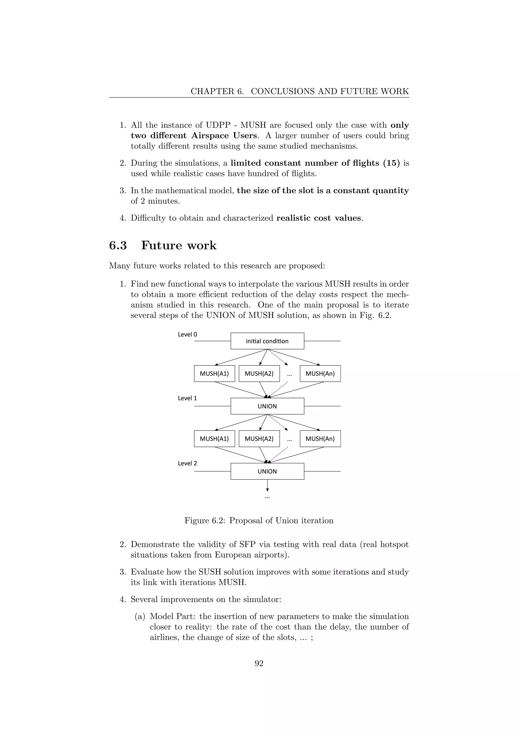
This document is a master's thesis from the University of Trieste focusing on optimal decision-making for air traffic slot allocation within a collaborative decision-making context. It explores various air traffic management mechanisms and models, including the Single User Single Hotspot (SUSH) and Multiple User Single Hotspot (MUSH) frameworks, and presents simulations and results to support the proposed methodologies. The final sections outline conclusions, limitations, and potential future work related to air traffic management optimization.
![List of Figures
1.1 CCS and hotspot . . . . . . . . . . . . . . . . . . . . . . . . . . . 12
1.2 Initial Arrival Time - Motivational Example . . . . . . . . . . . . 13
1.3 FPFS Scheduling - Motivational Example . . . . . . . . . . . . . 14
1.4 Swapping Scheduling - Motivational Example . . . . . . . . . . . 14
1.5 Research methodology . . . . . . . . . . . . . . . . . . . . . . . . 16
2.1 Gover Jack procedure, referring [4] . . . . . . . . . . . . . . . . . 19
2.2 Ration by Schedule and Compression procedures, referring [4] . . 20
2.3 Phases of SESAR project . . . . . . . . . . . . . . . . . . . . . . 21
2.4 Average care costs per delayed passenger, ref. [19] . . . . . . . . 23
2.5 Total passenger costs of delay per minute, ref. [19] . . . . . . . . 23
2.6 Graph passenger costs of delay per minute . . . . . . . . . . . . . 24
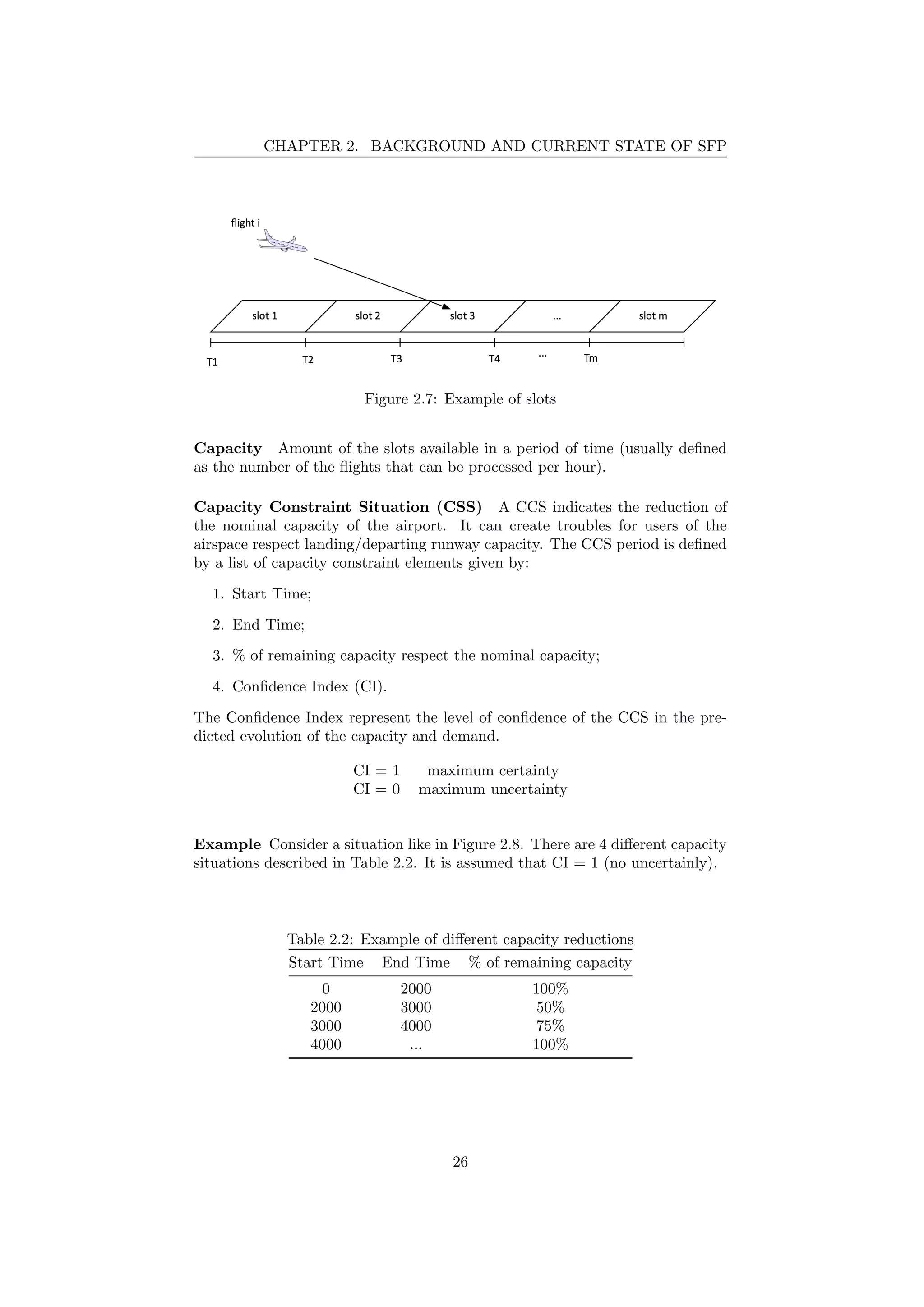
2.7 Example of slots . . . . . . . . . . . . . . . . . . . . . . . . . . . 26
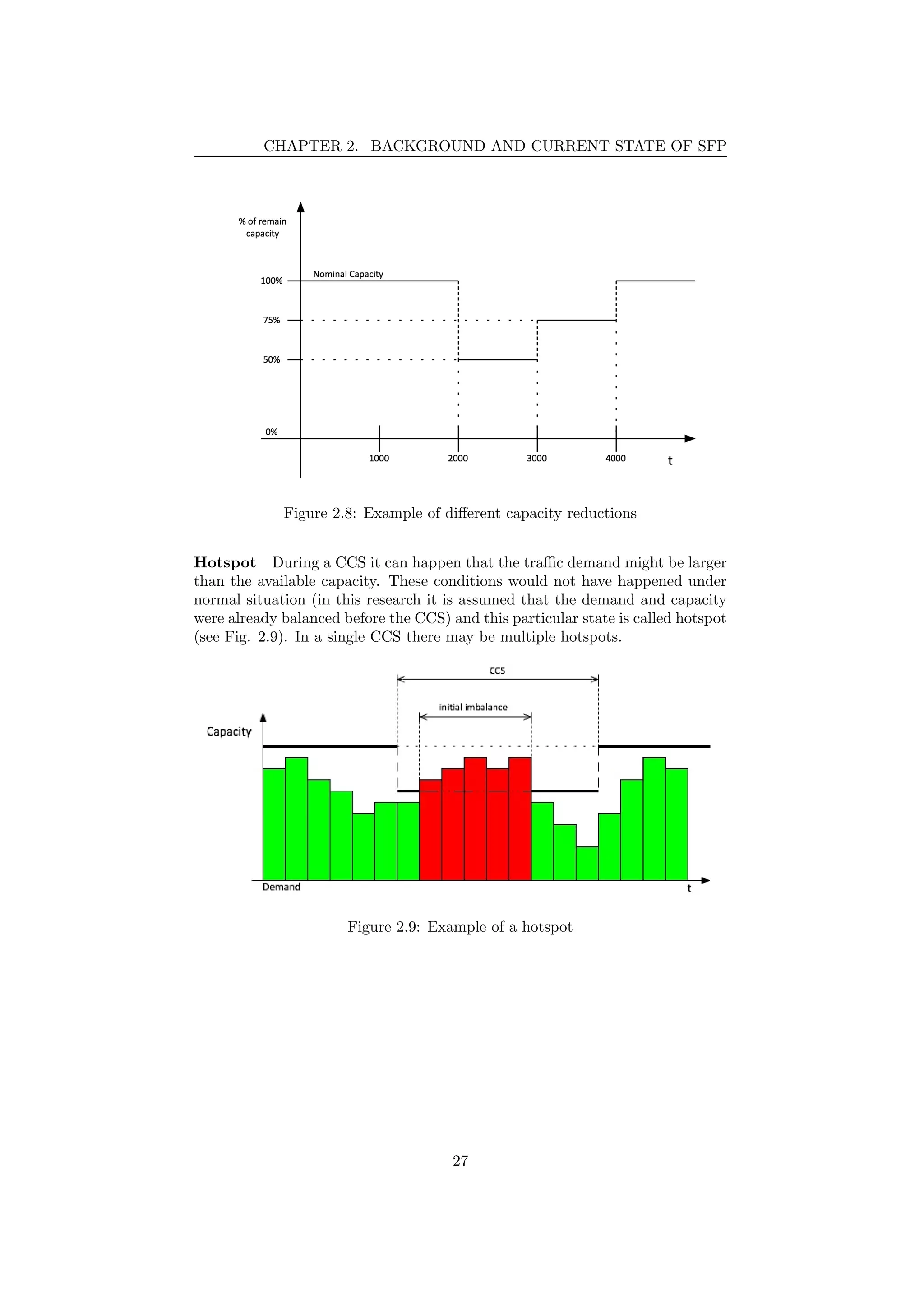
2.8 Example of different capacity reductions . . . . . . . . . . . . . . 27
2.9 Example of a hotspot . . . . . . . . . . . . . . . . . . . . . . . . 27
2.10 Stress and Recovery Period of a hotspot . . . . . . . . . . . . . . 28
2.11 Different cases of Hotspots . . . . . . . . . . . . . . . . . . . . . . 29
2.12 Different time requests . . . . . . . . . . . . . . . . . . . . . . . . 30
2.13 Initial condition - example 1 . . . . . . . . . . . . . . . . . . . . . 31
2.14 Suspension condition - example 1 . . . . . . . . . . . . . . . . . . 31
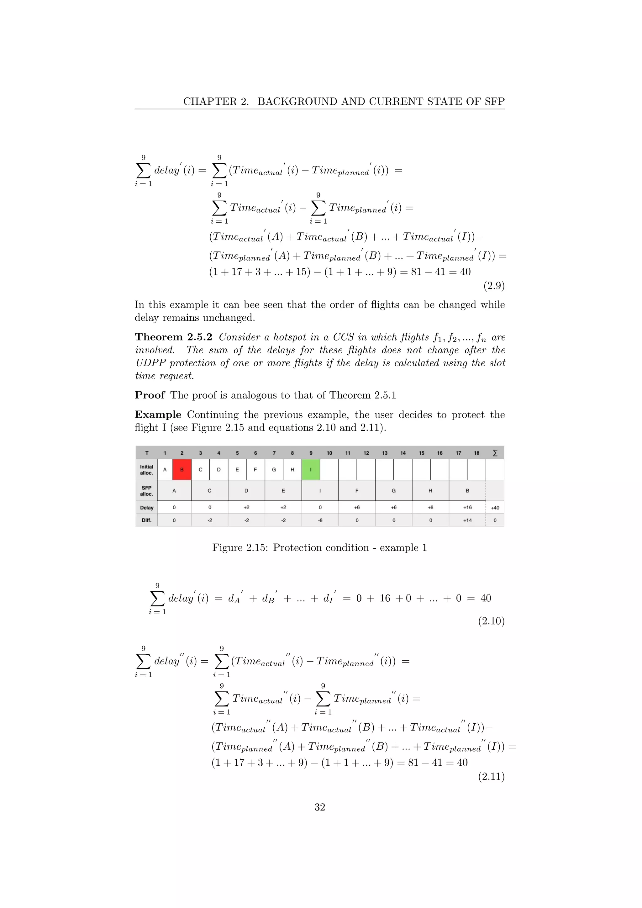
2.15 Protection condition - example 1 . . . . . . . . . . . . . . . . . . 32
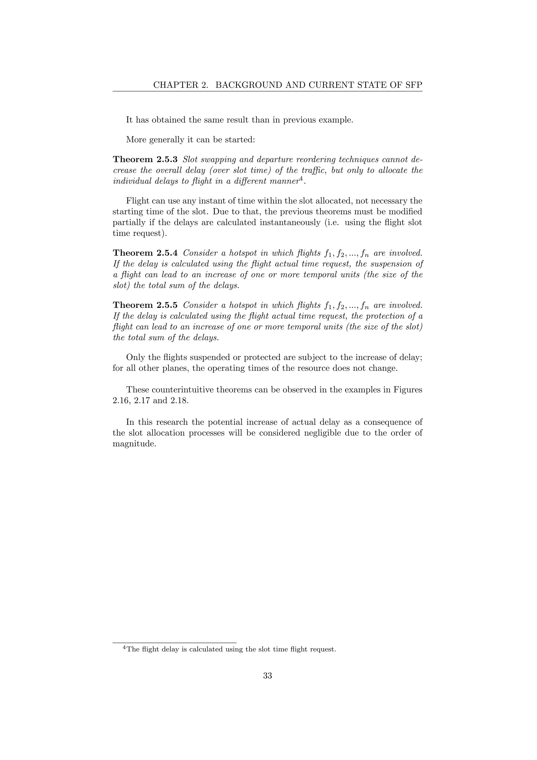
2.16 Changing of delay in suspension - slots size of 2 . . . . . . . . . . 34
2.17 Changing of delay in suspension - slots size of 3 . . . . . . . . . . 34
2.18 Changing of delay in protection - slots size of 2 . . . . . . . . . . 35
2.19 Graph of flights, slots and costs . . . . . . . . . . . . . . . . . . . 35
2.20 Initial condition - example 1 . . . . . . . . . . . . . . . . . . . . . 36
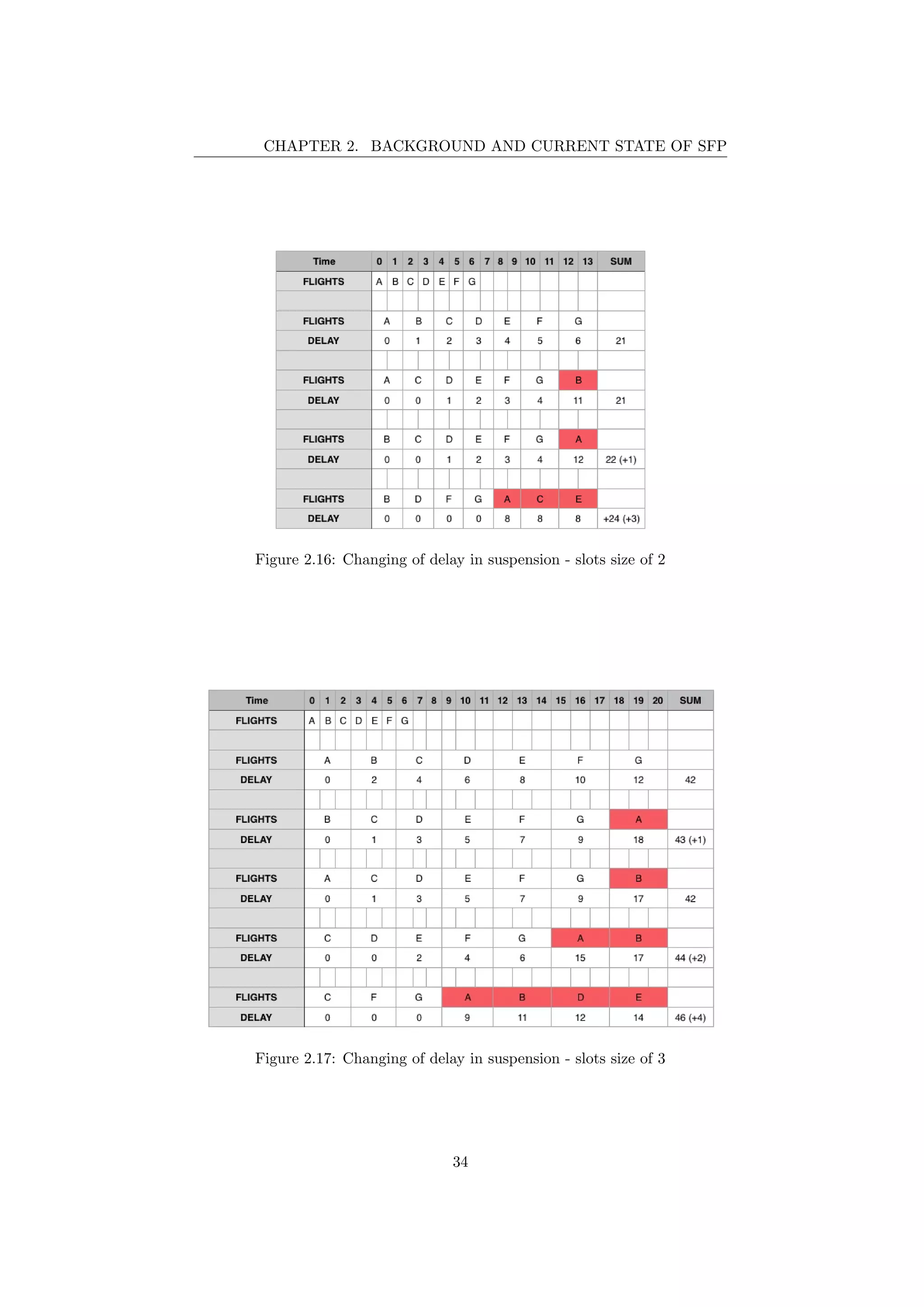
2.21 Initial condition graph - example 1 . . . . . . . . . . . . . . . . . 37
2.22 Suspension flight B - example 1 . . . . . . . . . . . . . . . . . . . 38
2.23 Suspension condition graph - example 1 . . . . . . . . . . . . . . 38
2.24 Protection of flight I - example 1 . . . . . . . . . . . . . . . . . . 39
2.25 Protection condition graph - example 1 . . . . . . . . . . . . . . 39
2.26 FPFS scheduling - example 2 . . . . . . . . . . . . . . . . . . . . 40
2.27 Suspension of flight B - example 2 . . . . . . . . . . . . . . . . . 41
2.28 Protection of flight E and I - example 2 . . . . . . . . . . . . . . 41
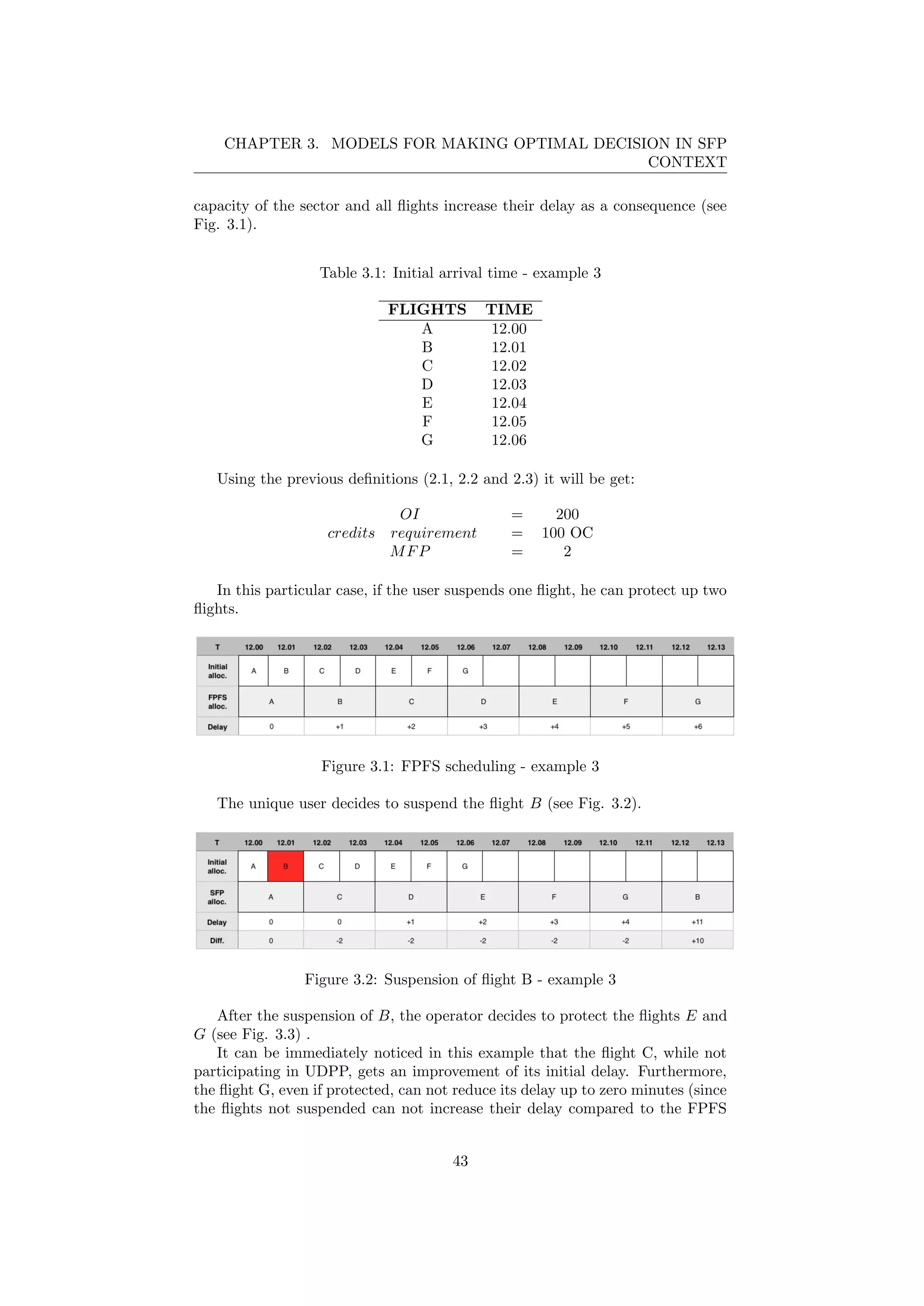
3.1 FPFS scheduling - example 3 . . . . . . . . . . . . . . . . . . . . 43
3.2 Suspension of flight B - example 3 . . . . . . . . . . . . . . . . . 43
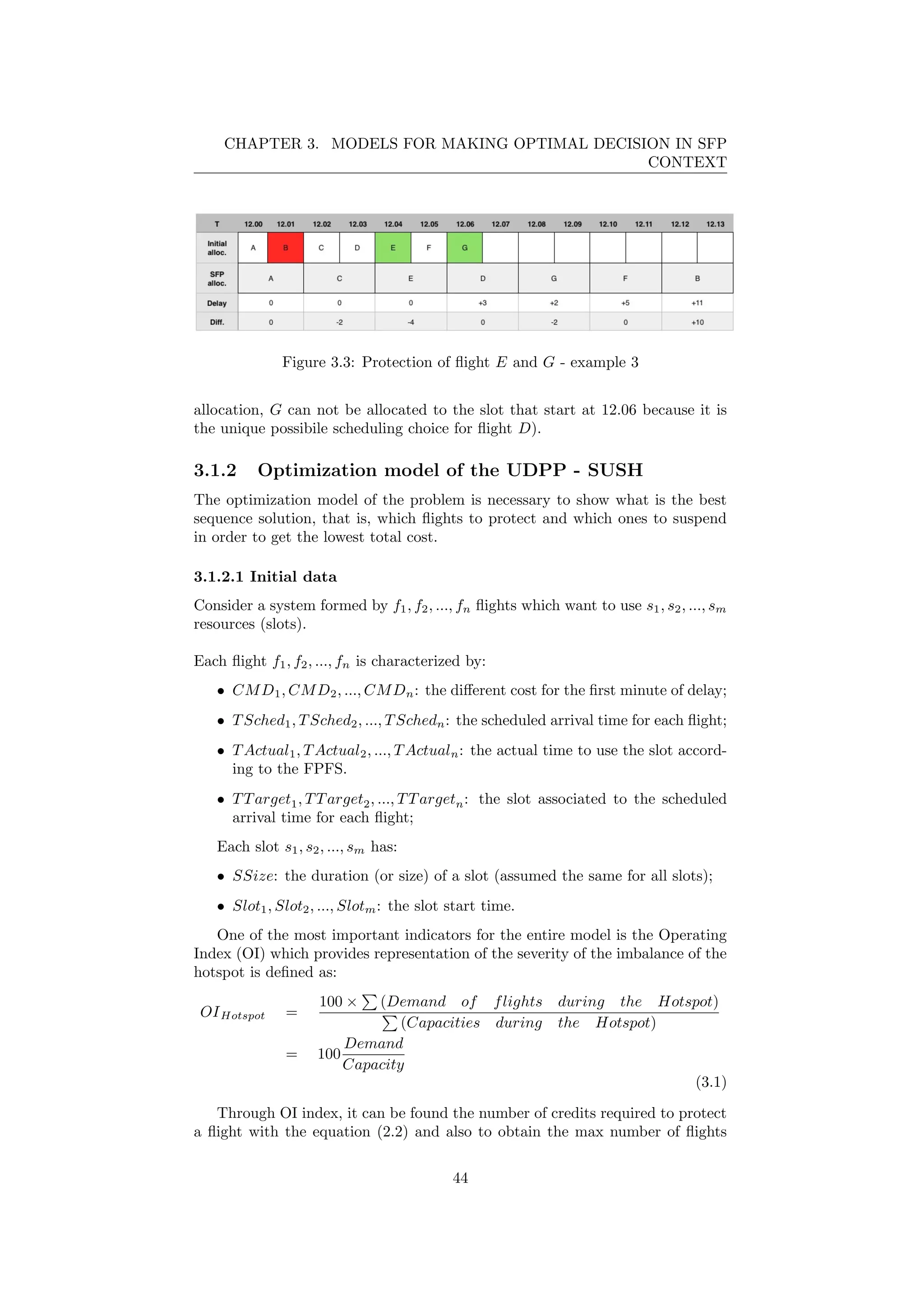
3.3 Protection of flight E and G - example 3 . . . . . . . . . . . . . . 44
3](https://image.slidesharecdn.com/tesi-160525173017/75/Optimal-decision-making-for-air-traffic-slot-allocation-in-a-Collaborative-Decision-Making-context-4-2048.jpg)


![Chapter 1
Introduction
In recent years the large amount of air traffic in Europe has led to a significant
increase in flight delays that become large costs for airlines (fuel, crew, taxes,
discontent of passengers, ...).
In 2014, around 880 million of passengers used the air transportation sys-
tem in Europe [1]. The United Kingdom reported the highest number of air
passengers in this period, with 220 million or an average of 3.4 passengers per
inhabitant (which was the double the EU-28 of passengers average). In Table
1.1 is shown the number of passengers in the busiest European airports for that
year (2014).
Table 1.1: The busiest airports in 2014
AIRPORT PASSENGERS
London Heathrow 73 million
Paris’ Charles de Gaulle 64 million
Frankfurt 59 million
Amsterdam’s Schiphol 55 million
After 2016, the traffic growth in Europe is estimated at around 2.6% increase
rate per year [2]. The 2008 peak of traffic of 10.1 million flights is forecasted to
be reached again in 2017. The new forecast is for 11.4 million IFR (Instrument
Flight Rules) movements in 2021, accounting for 19% more than in 2014.
These huge numbers are expected to keep growing exponentially in the in-
coming years and they represent the complexity of Air Traffic Management
(ATM) in Europe.
SESAR (Single European Sky ATM Research), with the aim of increasing
capacity but also to use the available capacity in a more efficient manner, de-
signed some solutions for this growing problem given the large amount of air
passengers.
This research is focused on creating an optimization model of one of the
mechanisms introduced by SESAR to manage the excess demand in reduced
capacity situation: User-Driven Prioritisation Process (UDPP).
The air traffic is planned and scheduled from several weeks ago up to a few
11](https://image.slidesharecdn.com/tesi-160525173017/75/Optimal-decision-making-for-air-traffic-slot-allocation-in-a-Collaborative-Decision-Making-context-12-2048.jpg)
![CHAPTER 1. INTRODUCTION
1.3 Methodology
In order to find the optimal decision making for AUs with respect to flight pri-
oritisation request in the context of SFP, a mathematical programming model is
developed in Section 3 in order to reflect the optimal operator behavior during
a hotspot.
The methodology is described in Fig.1.5: once the problem is observed, it is
followed by the development of a mathematical model. With the model, a set of
simulations can be performed in order to make predictions of the various cases
of the problem instances.
Figure 1.5: Research methodology
The main methodological steps in this research are:
1. Study of the Literature inherent to the UDPP;
2. Study of the Ground Delay Program (GDP) [4][11];
3. Development of linear programming model;
4. Design of the optimization mathematical model of UDPP-SUSH and UDPP-
SFP using the graph theory.
5. Implementation of the optimization mathematical model in FICO Xpress-
Optimizer [12], a commercial optimization solver for linear programming
(LP), thus obtaining a small software suite that manages the different
cases studied (FPFS - SUSH - MUSH).
6. Design and implementation of an agent-based simulator in JAVA in order
to study thousands of instances of the problem (Monte Carlo simulation2
).
7. Analyze the results and extract conclusions.
2Monte Carlo methods is a class of computational algorithms that use large random sam-
pling to obtain numerical results.
16](https://image.slidesharecdn.com/tesi-160525173017/75/Optimal-decision-making-for-air-traffic-slot-allocation-in-a-Collaborative-Decision-Making-context-17-2048.jpg)
![Chapter 2
Background and current
state of SFP
2.1 Current air traffic tactical slot allocation mech-
anisms
In Europe the Air Traffic Management (ATM) authority imposes a regulation
when there is imbalance between the requested demand and available capacity
which consists in forcing delays (Air Traffic Flow Management (ATFM) delays)
to some flights ([5],[25]). ATFM delays are imposed on a concept of equity but
without considering the Airspace User (AU) costs1
. The ATM authority then
manages flights through a First Planned First Served (FPFS) policy, which rep-
resent a fair procedure.
The Air Traffic Management authority focuses primarily on safety and capac-
ity to manage the various Airspace Users. Subsequently secondary objectives are
related to efficiency and costs and they are the ATM and flight cost-efficiency.
In order to manage these goals, Single European Sky ATM Research (SESAR)
has designed several procedures and mechanism which aim to manage the Euro-
pean ATM system (see Section 2.2.1), such as the Network collaborative man-
agement, dynamic demand, capacity balancing, airport integration in the ATM
network (Airport Collaborative Decision Making (A-CDM)), traffic synchro-
nization and 4D trajectory management.
2.1.1 Collaborative Decision Making in USA: Ground De-
lay Program
Interesting from a comparison viewpoint, the paradigm of Collaborative Deci-
sion Making in the USA is based on improving data exchange and communica-
tion between the Federal Aviation Administration (FAA) and the airlines, which
lead to better decision making. The primary focus of the CDM at the beginning
was the implementation of Ground Delay Program (GDP) enhancements. This
1The UDPP-SFP mechanism instead manages the various costs for users while maintaining
the concept of fairness and increasing flexibility for the AUs.
18](https://image.slidesharecdn.com/tesi-160525173017/75/Optimal-decision-making-for-air-traffic-slot-allocation-in-a-Collaborative-Decision-Making-context-19-2048.jpg)
![CHAPTER 2. BACKGROUND AND CURRENT STATE OF SFP
procedure is usually instantiated when one of the following events occur at the
airport:
• bad weather;
• an aircraft incident;
• closed runways;
• a large volume of aircraft going to an airport;
• a large volume of aircraft going en route to another airport in the same
line of flight;
• a condition that requires increased spacing between aircraft (such as the
Instrument Landing System (ILS) approaches vs. Visual Flight Rules
(VFR) approaches).
In the Ground Delay Program flights that are scheduled to arrive during
periods of congestion are assigned delays prior to their departure (it is assumed
that is less expensive and safer to delay a flight on the ground than in airborne).
This type of allocation can be viewed as a resource allocation problem, i.e.: the
available arrival capacity (arrival slots) is allocated to flights (and a new depar-
ture slot is allocated to flights). The central idea of GDP is to manage delays
and cancellations of flights to optimize the scheduling with special procedures.
2.3.3.2 GDP procedures
Before the implementation of GDP flights were assigned to slots by a First Come
First Served (FCFS) algorithm known as Grover Jack. The affected flights were
ordered according to their most recent estimated arrival times. This method of
assigning flights to slots penalized the airlines for providing accurate information
(if a flight delay increases and this is not communicated, the aircraft preserves
the same slot).
Figure 2.1: Gover Jack procedure, referring [4]
The new idea of the GDP paradigm is to consider the allocation of capacity to
an assignment of slots to airlines. This has led to two new mechanisms, called
Ration-By-Schedule (RBS) and Compression. The RBS algorithm generates
the initial allocation of slots to airlines, based on the recognition that airlines
have claims on the arrival capacity through the original flight schedules. FAA
periodically execute Compression: an algorithm that updates the schedule by
an inter-airline slot exchange, which aims to provide airlines with an incentive to
report flight cancelations and delays (unlike the Gover Jack procedure). Airlines
can adjust their schedules by substituting and canceling flights.
19](https://image.slidesharecdn.com/tesi-160525173017/75/Optimal-decision-making-for-air-traffic-slot-allocation-in-a-Collaborative-Decision-Making-context-20-2048.jpg)
![CHAPTER 2. BACKGROUND AND CURRENT STATE OF SFP
Figure 2.2: Ration by Schedule and Compression procedures, referring [4]
2.2 SESAR
The European Commission (EC) developed in 1999 a legislative framework for
European aviation to manage the dramatic growth in the air travel. The pre-
vious airspace design driven by national boundaries are expected to merge into
airspace blocks to maximize the efficiency of the airspace. Air Traffic Manage-
ment will be driven by the requirements of the airspace user and the need to
provide for increasing air traffic beyond the primary objective of safety.
In 2004 Single European Sky sets up the Single European Sky ATM Re-
search (SESAR) project to define ATM systems through definitions, develop-
ments and deployments of new solutions, called SESAR Solutions.
SESAR is the EU-wide framework whose High-Level Goals are described in
Table 2.1 [3].
Table 2.1: SESAR goals
GOAL DESCRIPTION
CAPACITY
enable a threefold increase in capacity which will also reduce
delays both on the ground and in the air
SAFETY improve safety by a factor of 10
ENVIRONMENT 10% reduction in the effects flights have on the environment
COST
provide ATM services to airspace users at a cost of at least 50 %
less
SESAR contributes to these High-Level Goals managing the resources of the
entire ATM community, including:
• the Network Manager (NM)2
;
• civil and military air navigation service providers (ANSPs);
• airports and military aerodromes opened to civil air traffic;
• civil and military airspace users;
• staff associations;
• academia;
• research centers.
2EUROCONTROL, https://www.eurocontrol.int
20](https://image.slidesharecdn.com/tesi-160525173017/75/Optimal-decision-making-for-air-traffic-slot-allocation-in-a-Collaborative-Decision-Making-context-21-2048.jpg)
![CHAPTER 2. BACKGROUND AND CURRENT STATE OF SFP
SESAR project is composed by 3 different phases [6]:
1. Definition phase (2005 − 2008). This phase was characterized by differ-
ent goals :
• define European air transport system performance requirements up
to 2020 and beyond;
• identify globally interoperable ATM solutions;
• produce the detailed research and technology work programme;
• propose the legislative, financial and regulatory framework;
• establish a detailed deployment plan.
This phase was co-financed by the European Commission (through the
Trans-European Transport Network (TEN-T) programme) and EURO-
CONTROL. Its total cost was 60 million Euro (50% European Commis-
sion, 50% EUROCONTROL).
2. Development phase (2008 − 2016). This phase is managed by the
SESAR Joint Undertaking 3
: a joint undertaking created under European
Community law on 27th of February 2007. SESAR Joint Undertaking
produced the required new generation of technological systems, compo-
nents and operational procedures as defined in the SESAR ATM Master
Plan and Work Program. Its total cost is 2.1 Billion Euro (1/3 European
Commission, 1/3 EUROCONTROL, 1/3 Industries).
3. Deployment phase (2014−2020). It will be a large-scale production and
implementation of the new air traffic management infrastructure composed
of interoperable components guaranteeing high performance air transport
activities. It will cost 20 Billion Euro paid by the Industry.
Figure 2.3: Phases of SESAR project
The SESAR Solution are operational and technological improvements which
aim to manage the European ATM system. The concept of operations is based
on the following topics:
• Moving from airspace to 4D trajectory management allows the
sharing of aircraft trajectories between all the ATM users. Airspace Users
(AU) and Air Navigation Service Providers (ANSP) have the same view
of all the flights in the system. They can have the the most up-to-date
data available to perform their tasks therefore it let dynamic adjustment
aircraft trajectories or scheduling.
3SESAR Joint Undertaking, http://www.sesarju.eu.
21](https://image.slidesharecdn.com/tesi-160525173017/75/Optimal-decision-making-for-air-traffic-slot-allocation-in-a-Collaborative-Decision-Making-context-22-2048.jpg)
![CHAPTER 2. BACKGROUND AND CURRENT STATE OF SFP
• Traffic synchronization aims to reach an optimum traffic sequence:
optimize the sequencing of aircraft surface movements, arrivals and de-
partures at airports so to avoid the Air Traffic Control (ATC) tactical
intervention.
• Network collaborative management, dynamic demand and ca-
pacity balancing aim different phases of operation planning from long
to medium/short term. All users of the system progressively share more
and more precise data to build a common traffic and operational envi-
ronment picture: the Network Operations Plan (NOP)[14]. This topic is
closely related to the first argument: 4D Trajectory which is a first ex-
ample of sharing precise data in the entire system. The Collaborative
Decision Making (CDM) and the User Driven Priorisation Process
(UDPP) are part of this topic. During periods of imbalance between de-
mand and capacity in particular sector of ATM, the process UDPP will
be activated: users can negotiate together and make proposal to change
the scheduling of flights to manage the critical condition in an efficient
and equitable way.
• Airport integration and throughput aims a full integration of airports
into the ATM network. An important topic of SESAR is the implementa-
tion of Airport Collaborative Decision Making (A-CDM) which improves
Air Traffic Flow and Capacity Management (ATFCM) at airports reduc-
ing delays and improving the predictability and efficiency.
• Conflict management and automation aims at reducing controller
task load per flight through a increment of integrated automation support.
Air Navigation Service Provider (ANSP) and pilots will be assisted by new
automated functions to handle decision-making processes.
• System Wide Information Management (SWIM) consists of new
standards, infrastructure and governance enabling the management of
ATM information. It is a complete change in the way of how informa-
tion is managed along its lifecycle: the future European ATM intranet.
2.3 Cost of delay
One of the main objectives of SESAR is to reduce the various costs for Airspace
Users, as shown in Table 2.1. One of the major costs that SESAR aims at
reducing is the cost of delay.
The actual cost of delay of a particular flight depends on many factors and it
is difficult to know it with exactitude even for the operator of the flight. However
it is possible to approximate these costs through statistical characterization. In
[19] some reference values are given.
The cost of delay can be split in two sides: hard and soft costs.
Hard are those costs resulting from passenger delay, such as those due to pas-
senger rebooking, compensation and care. Table 2.4 shows reference values (ref.
[19]) of different care costs per passenger for different hours of delay.
22](https://image.slidesharecdn.com/tesi-160525173017/75/Optimal-decision-making-for-air-traffic-slot-allocation-in-a-Collaborative-Decision-Making-context-23-2048.jpg)
![CHAPTER 2. BACKGROUND AND CURRENT STATE OF SFP
Figure 2.4: Average care costs per delayed passenger, ref. [19]
Soft costs manifest in several ways, for example as follow:
• A passenger with a flexible ticket may arrive at an airport and decide to
take a competitors on-time flight instead of a delayed flight.
• Passengers may perceive the airline unpunctual and choose another.
• Due to a delay, a passenger may defect from an unpunctual airline as a
result of dissatisfaction.
Soft costs are rather more difficult to quantify, but may even overcome the
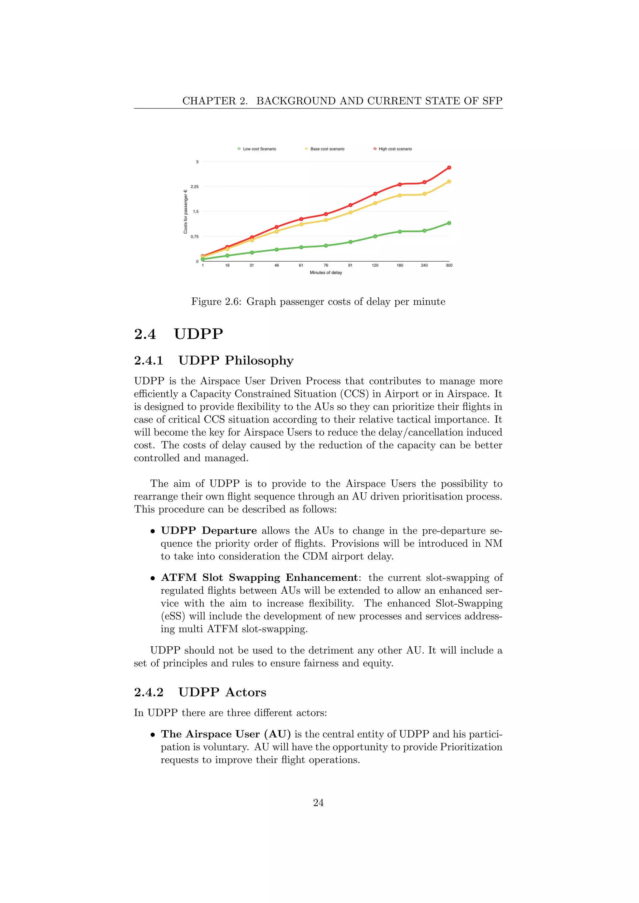
hard costs. Longer delays have higher associated costs per minute. This fact,
together with the different absolute values of the delay cost for each individual
flight, can be described by a particular function of costs, similar to that in
Figure 2.5 (these three different functions are made using the data in Table 2.6
that represents the costs of delay in three different scenarios (low, normal and
high cost scenario), [19]).
Figure 2.5: Total passenger costs of delay per minute, ref. [19]
23](https://image.slidesharecdn.com/tesi-160525173017/75/Optimal-decision-making-for-air-traffic-slot-allocation-in-a-Collaborative-Decision-Making-context-24-2048.jpg)
![CHAPTER 2. BACKGROUND AND CURRENT STATE OF SFP
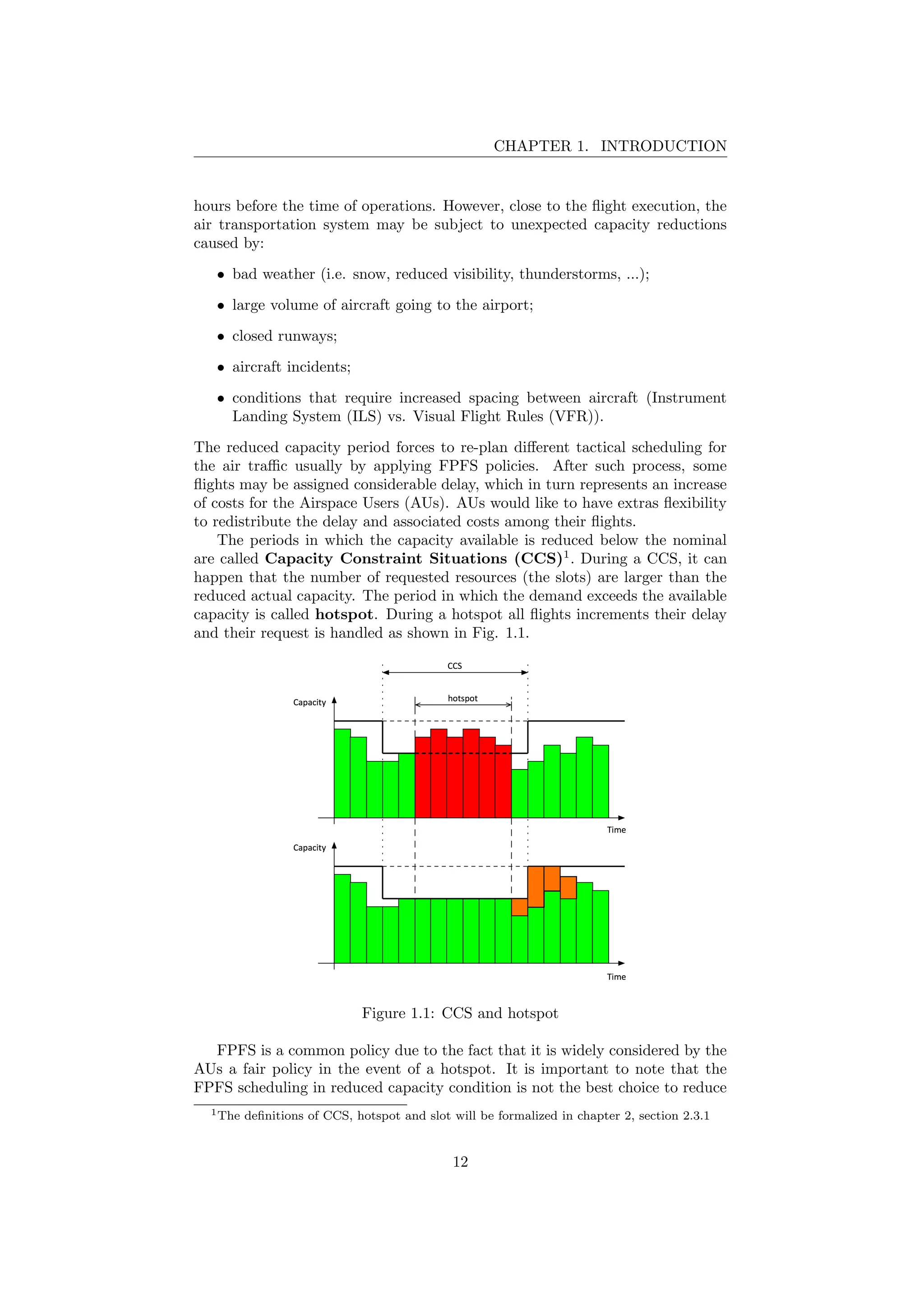
The excess demand during hotspots must be managed and spread (by ap-
plying delays to individual flights) to handle all the requests for slot allocation.
There are therefore two different periods during hotspots [22]:
1. Stress Period: period of time in which there is an imbalance between
demand and capacity (there is an excess of demand) and the trend of the
average of the delay is growing.
2. Recovery Period: period of time in which there is a free slot where the
last flight of the excess demand can be allocated and therefore the sector
is no longer under stress (the excess demand is fully absorbed).
Figure 2.10: Stress and Recovery Period of a hotspot
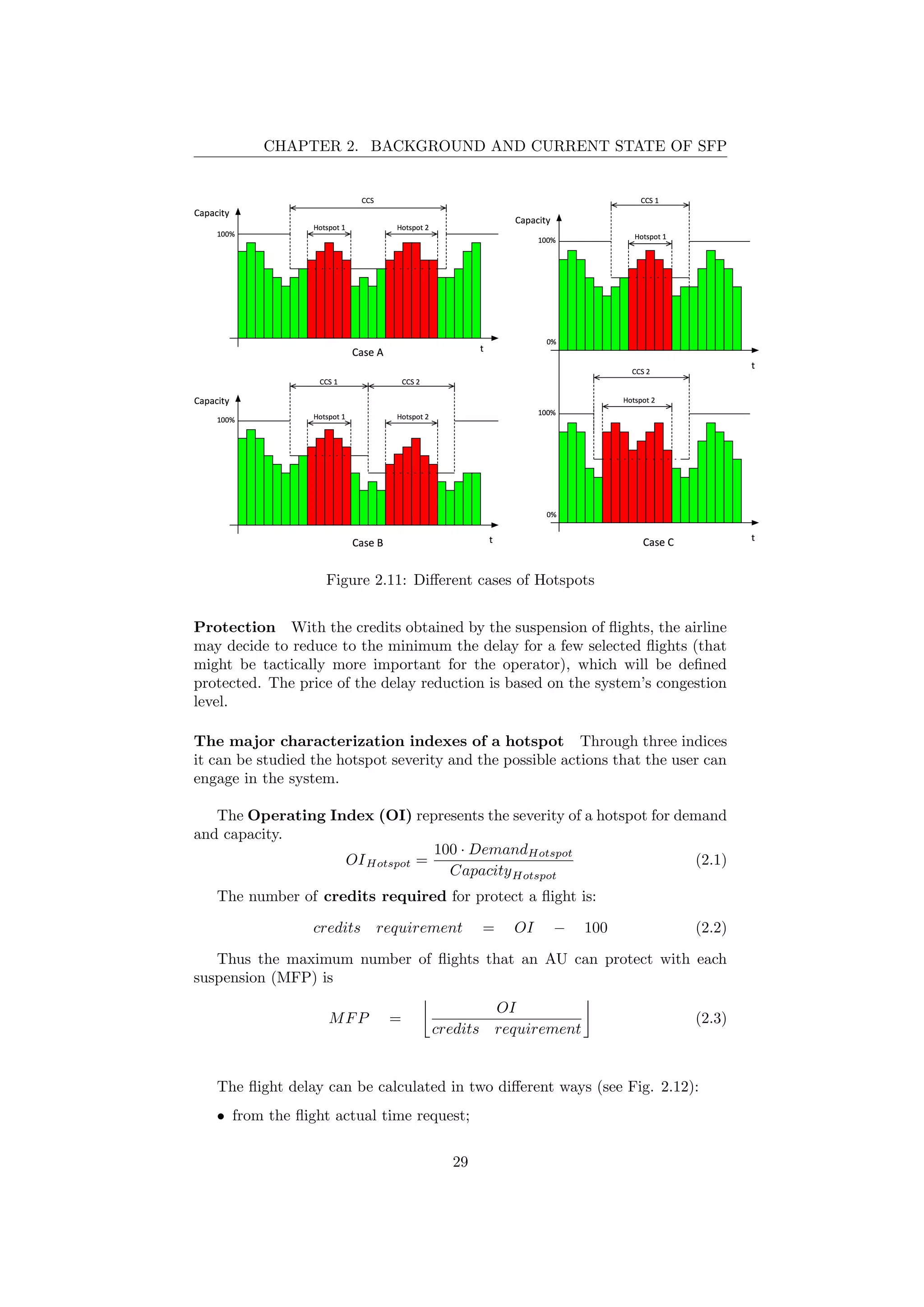
It can be considered also a situation with multiple hotspots. These can be
included in one or more CSSs, as it can be seen in Figure 2.11. In this research
only single hotspot will be considered. Furthermore will not be studied the po-
tential interdependencies between hotspots.
There are three different connections between hotspots and CSSs:
(A) There may be two or more hotspots in the same CCS;
(B) There may be two or more hotspots in different CSSs in the same geograph-
ical area (eg. the same track, the same airport, ...).
(C) There may be two or more hotspots in different CCSs in different territorial
areas (eg. two or more different airports).
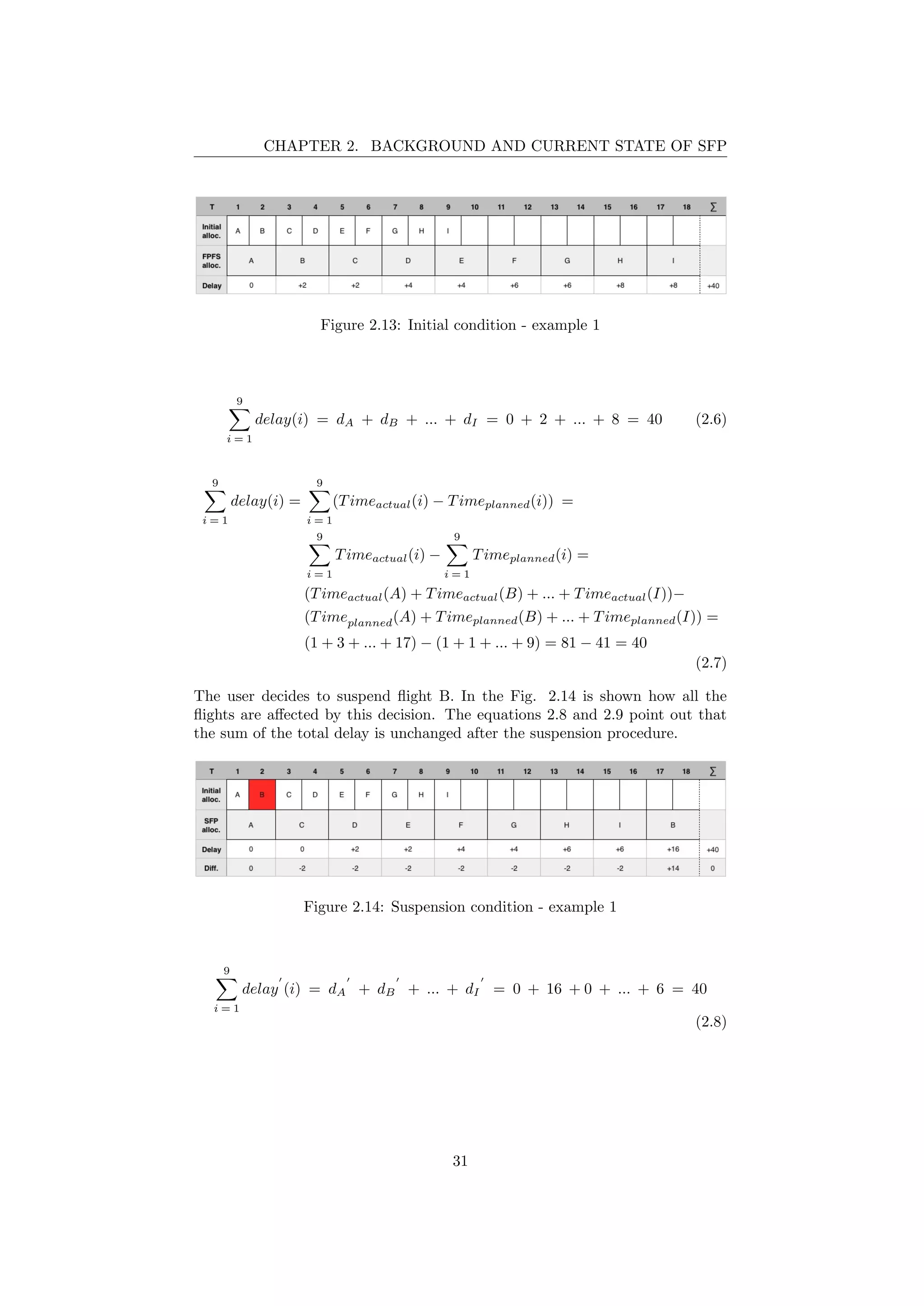
Suspension One of the basic SFP procedure tasks is the suspension of a flight.
An airline can decide to increase the delay of one of its flights until the end of
the hotspot area; for each suspended flight, the flight operator can manage 100
credits for prioritization rights.
28](https://image.slidesharecdn.com/tesi-160525173017/75/Optimal-decision-making-for-air-traffic-slot-allocation-in-a-Collaborative-Decision-Making-context-29-2048.jpg)
![CHAPTER 2. BACKGROUND AND CURRENT STATE OF SFP
• from the flight slot time request.
Figure 2.12: Different time requests
In this research it is assumed that a flight whose its initial scheduling time
is in the middle of a slot due to a capacity reduction, it can be associated to
that slot with a delay of zero minutes (no negative delays). For example in the
Fig. 2.12 the considered flight will be allocated in the slot i.
These two calculation methods lead to different consequences regarding the
change of the total sum of the minutes delay of the flights, explained in Theorems
2.4.1, 2.4.2, 2.4.3, 2.4.4 and 2.4.5.
Theorem 2.5.1 Consider a hotspot in a CCS in which flights f1, f2, ..., fn are
involved. The sum of the delays for these flights does not change after the UDPP
suspension of one or more flights if the delay is calculated using the slot time
request.
Proof Notice that the delay of a single flight is defined as the sum of the actual
flight arrival time minus its scheduled arrival (slot) time so:
n
i=1
delay(i) =
n
i=1
(Timeactual − Timeplanned) (2.4)
Consider the two different part that form the delay
n
i=1
delay(i) =
n
i=1
(Timeactual) −
n
i=1
(Timeplanned) (2.5)
The summation of the planned flight (slot) time doesn’t change after a suspen-
sion because it is constant in time. Instead the sort of the actual flight times is
different but the sum remains unchanged. So the final sum of the delays remains
the same after a suspension procedure.
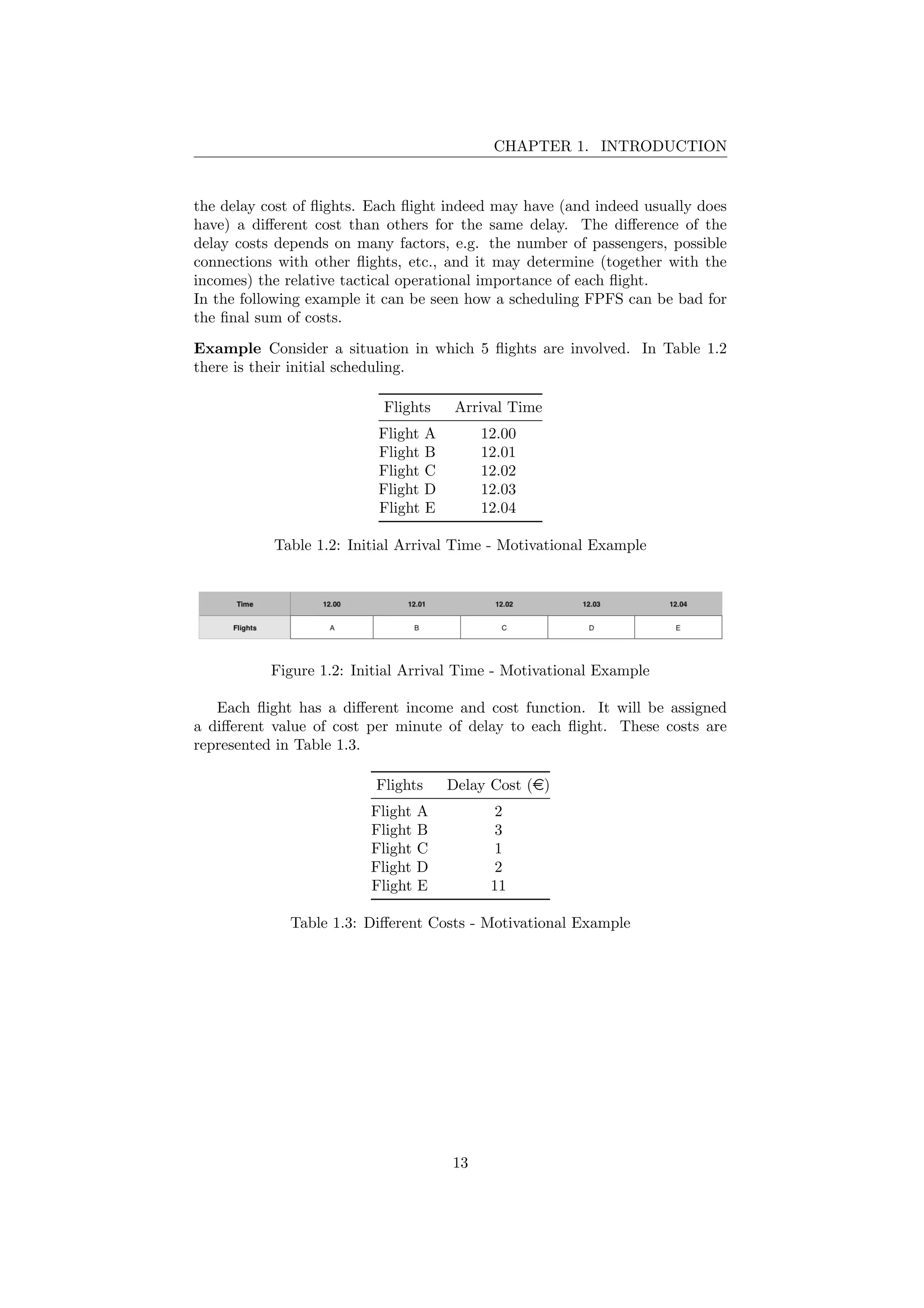
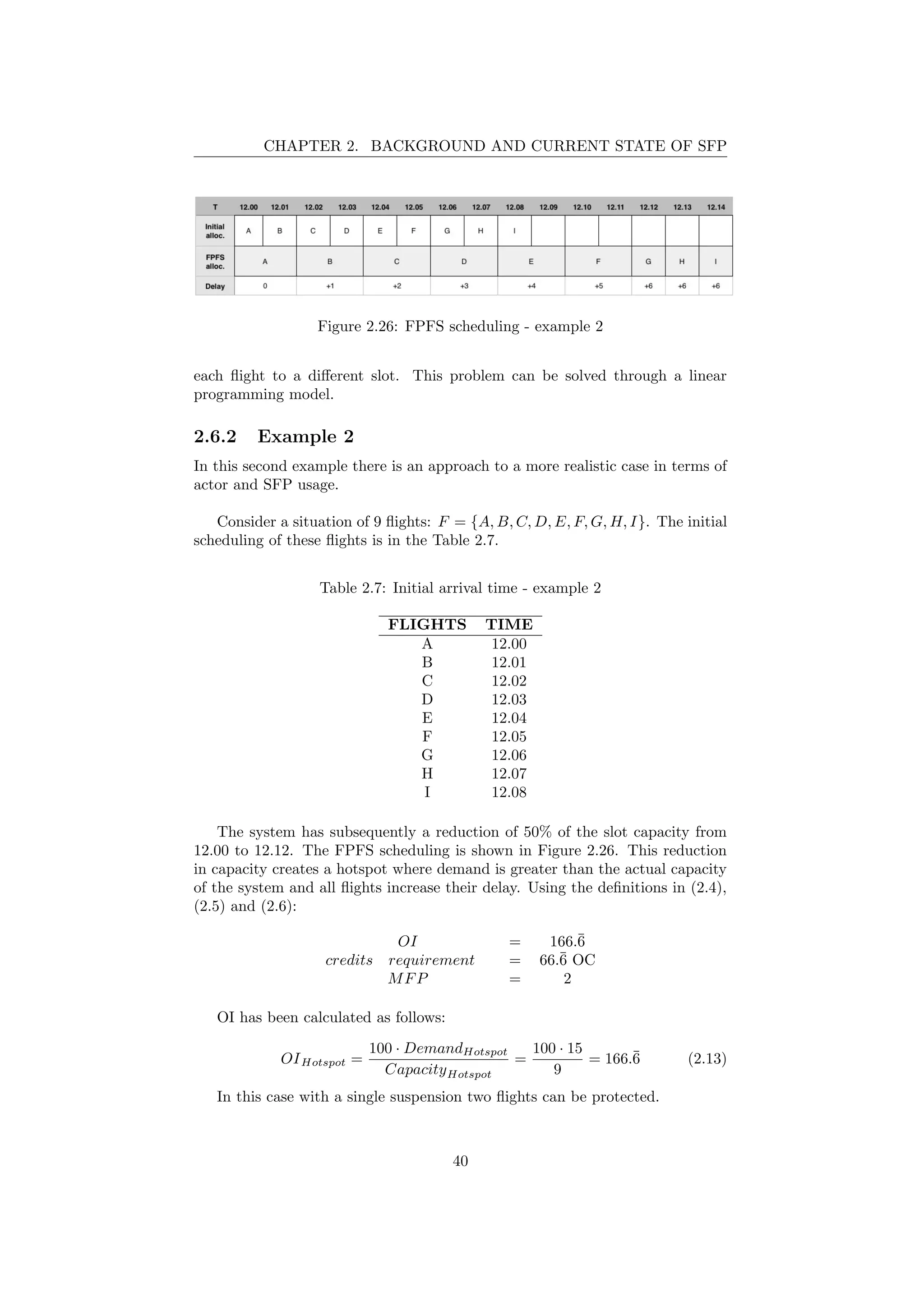
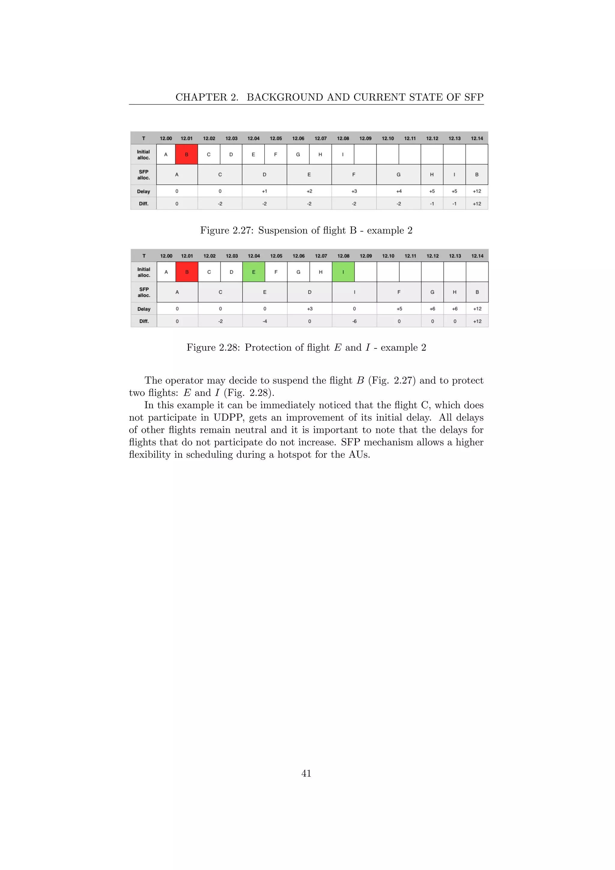
Example Consider the following example. Such scenario is characterized by a
set of 9 flights, F = {A, B, C, D, E, F, G, H, I}, that configures the slot demand
over a period of t = [1, 9] with a capacity reduction of the 50% for the period
(slot size of 2 minutes). In this example the sum of all the total delays in FPFS
scheduling is 40 minutes (see equations 2.6 and 2.7). In Figure 2.13 is shown the
different flights slots allocation between the initial situation and FPFS schedul-
ing.
30](https://image.slidesharecdn.com/tesi-160525173017/75/Optimal-decision-making-for-air-traffic-slot-allocation-in-a-Collaborative-Decision-Making-context-31-2048.jpg)
![CHAPTER 2. BACKGROUND AND CURRENT STATE OF SFP
Figure 2.18: Changing of delay in protection - slots size of 2
2.6 Selective Flight Protection optimization prob-
lem
This Selective Flight Protection optimization problem can be thought as a graph
problem [17]. The entities that fill the system are the flights, slots and the costs
of each flight for each slot. The entire system can be thought as a graph with
two types of vertices: flights and slots. The weight of the arcs that connect that
vertices are the costs5
(see Fig. 2.19).
Figure 2.19: Graph of flights, slots and costs
5i.e. the cost ci,j
35](https://image.slidesharecdn.com/tesi-160525173017/75/Optimal-decision-making-for-air-traffic-slot-allocation-in-a-Collaborative-Decision-Making-context-36-2048.jpg)
![CHAPTER 2. BACKGROUND AND CURRENT STATE OF SFP
Table 2.3: Initial arrival time - example 1
FLIGHTS TIME
A 1
B 2
C 3
D 4
E 5
F 6
G 7
H 8
I 9
Each arc has a weight and the goal of the optimal procedure is to find the
right set of arcs that minimizes costs for the entire system and connect each
flight to a different slot. It is important to highlight that usually not all flights
can be connected to every slots: this link depends on the flight arrival time and
the slot actual time. This concept will be further discussed in the Chapter 3.
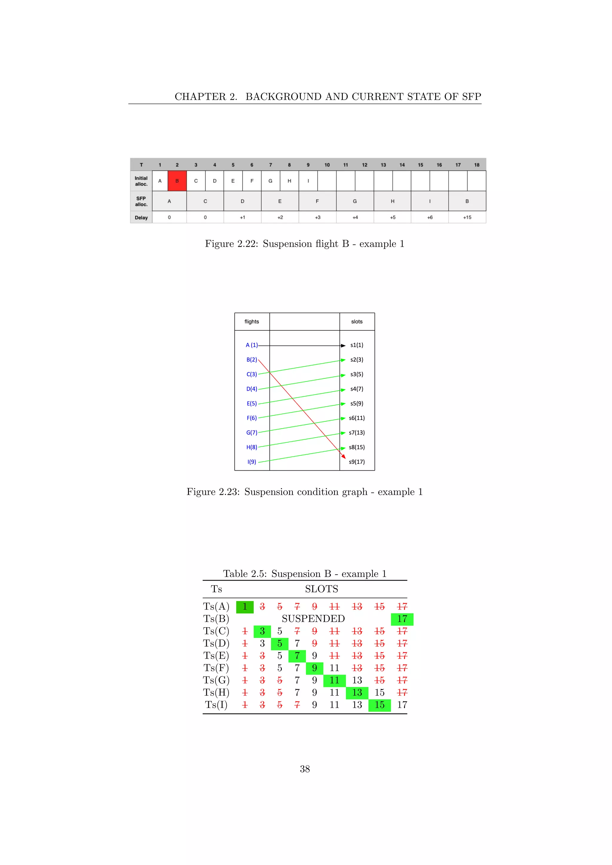
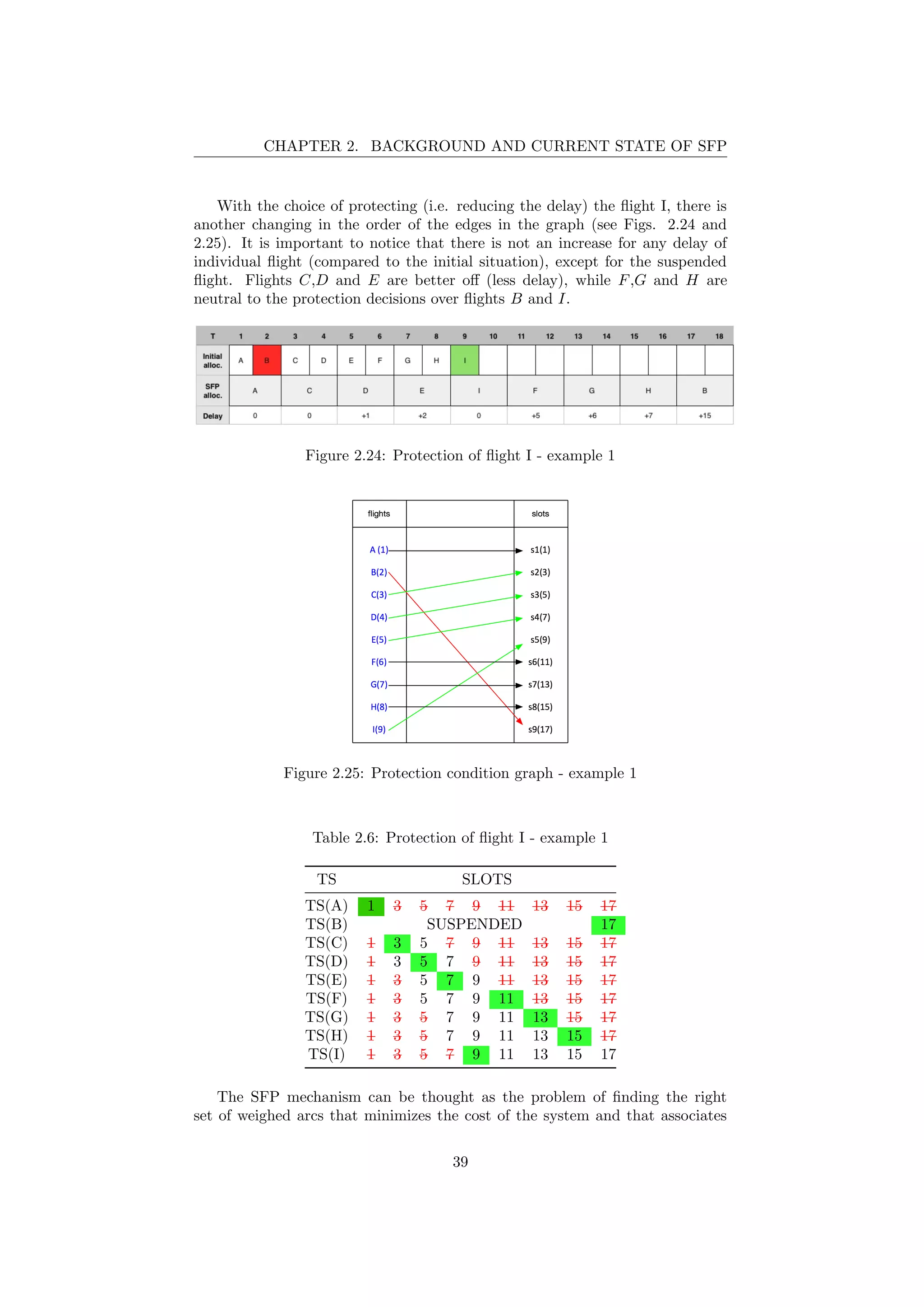
2.6.1 Example 1
Using the above representation, a scenario will be described in which 9 flights
F = {A, B, C, D, E, F, G, H, I} are involved over a period of t = [1, 9] (see Fig.
2.20). Their scheduled time is in Table 2.3. Assume there is a capacity reduction
of the 50% so the flights can no longer use the resources every minute. The
operator, using SFP mechanism, decides to suspend the flight B and to reduce
as much as possible the delay of the flight I.
Figure 2.20: Initial condition - example 1
In Figure 2.21, there is the graph representation of this problem example.
The blue nodes are the flights (in the parenthesis there is the scheduled time)
and the black nodes instead represent the slots (in the parenthesis there is the
new allocated time).
In Table 2.4, Ts is the set of slots that flights are willing to accept in ex-
change for the actual slot.
36](https://image.slidesharecdn.com/tesi-160525173017/75/Optimal-decision-making-for-air-traffic-slot-allocation-in-a-Collaborative-Decision-Making-context-37-2048.jpg)
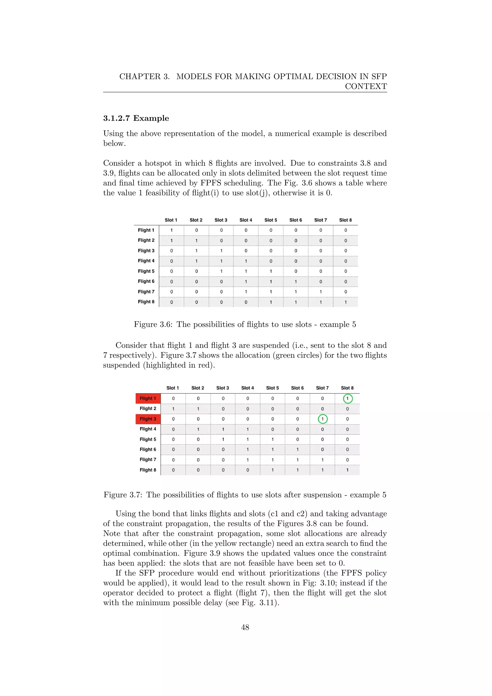
![CHAPTER 3. MODELS FOR MAKING OPTIMAL DECISION IN SFP
CONTEXT
that can be protected from a single suspension MFP.
Each flight has a different delay for every sequence position in the hotspot.
The matrix d(i, j) represent these values.
d(i, j)
i in 1..n, j in 1..m
= delay for flight fi in slot sj (3.2)
3.1.2.2 The decisional variables
The binary decisional variable is x(i, j).
x(i, j)
i in 1...n, j in 1...m
=
1 if flight fi use slot sj
0 otherwise
(3.3)
All the flights can be divided in normal [n], protected [p] and suspended [s]
ones so three new binary variables are introduced.
flights =
normal flights
protected flights
suspended flights
(3.4)
3.1.2.3 The objective function
The objective function of the model is to minimize the costs for all the AUs.
minimize
i in 1...n, j in 1...m
x(i, j) · d(i, j) · f(d(i, j)) · CMD(i) (3.5)
f(d(i, j)) is a function used to calculate the flight cost due to the delay. In
the implementation of the simulator it will be used a pseudo-real cost function
found through Cook, Tanner, Jovanovic, Lawes studies about the cost of delay
to air transport in Europe [19] (see Section 5.1.2).
3.1.2.4 The constraints
Constraint c1: ”Each flight must have one and only one slot allocated”.
∀ i
i in 1..n
j in 1..m
x(i, j) = 1 (3.6)
Constraint c2: ”Each slot cannot be allocated to more than a single flight”.
∀ j
j in 1..m
i in 1..n
x(i, j) ≤ 1 (3.7)
Constraint c3: ”Each flight is normal [n] or protected [p] or suspended [s]”.
∀ i
i in 1..n
n(i) + p(i) + s(i) = 1 (3.8)
45](https://image.slidesharecdn.com/tesi-160525173017/75/Optimal-decision-making-for-air-traffic-slot-allocation-in-a-Collaborative-Decision-Making-context-46-2048.jpg)
![CHAPTER 3. MODELS FOR MAKING OPTIMAL DECISION IN SFP
CONTEXT
Constraint c4: ”The delay of each flight, except for the suspended ones, must
be between 0 minutes and the FPFS scheduling delay”.
if delayactual(i) > delayF P F S(i) ⇒ x(i, j) ≤ s(i)
for every i in 1...n, j in 1...m
(3.9)
Constraint c5: ”The suspended flights are scheduled in the last position of
the hotspot”.
In order to highlight which are the suspended flights it will be checked if the
flight increases its delay more than the FPFS baseline delay. If so, it must be a
suspended flight.
if delayactual(i) > delayF P F S(i) ⇒ s(i) = 1
for every i in 1...n
(3.10)
There is a vector r indicating the possible position of the flights suspended at
the end of the optimization. It will be formed as follows: r : [0, ..., 0, 1, ..., 1]
(suspended flights can be placed only on the last hotspot position). The num-
ber of 1 in the vector is equal to the sum of flights suspended in the sector.
if s(i) = 1 ⇒ x(i, j) · s(i) · r(j) = 1
for every i in 1...n, j in 1...m
(3.11)
Constraint c6: ”The number of credits for every operator cannot be negative
(i.e., proportional effort is required first before any flight protection)”.
Cr ≥ 0 (3.12)
Constraint c7: ”The protected flights will be scheduled in their best possible
position (least possible delay)”.
To find out which flights are protected compared to non-prioritized flights, it
will be introduced a new vector h. It represents the amount of delay improved
due to the suspension for the individual flights. In the following example there
will be a practical representation of how the vector h is made and how it behaves
due to flight suspensions.
Example Consider a case in which 5 flights F = {A, B, C, D, E} are involved
in a situation of 50% reduction of sector capacity. In Figure 3.4 is shown the
FPFS scheduling.
Figure 3.4: FPFS scheduling - example 4
The operator decides to suspend the flights B and D, as shown in Fig. 3.5.
46](https://image.slidesharecdn.com/tesi-160525173017/75/Optimal-decision-making-for-air-traffic-slot-allocation-in-a-Collaborative-Decision-Making-context-47-2048.jpg)
![CHAPTER 3. MODELS FOR MAKING OPTIMAL DECISION IN SFP
CONTEXT
Figure 3.5: Suspension of B and D - example 4
The vector h, that represents in a system without protection the change of
the non-prioritized flight delay, in this example is: h : [0, s, 2, s, 4] (the letter s
represents the suspended flights).
The non-prioritized flights in this particular instance are A, C and E, re-
spectively the first, the third and the fifth position of the vector h.
If a flight has a larger reduction of the delay than the corresponding value in
h, it has been protected: its delay reduction is larger than the non-prioritized
flights reduction.
if(−∆delay(i) > h(i)) ⇒ p(i) = 1
for every i in 1...n
(3.13)
3.1.2.5 The definitions
Definition d1: with a flight suspension, the user gets 100 OC and these credits
are included in its total budget.
Budget = 100 ·
i in 1,...,n
s(i) (3.14)
Definition d2: The amount of credits to protect the flights are:
Credits spent = [OI − 100] ·
i in flights
p(i) (3.15)
These credits can be used in order to prioritize certain flights.
Definition d3: d1 and d2 can be combined to calculate the residual value
of the user’s credits .
Cr = 100 ·
i in flights
s(i) − [OI − 100] ·
i in flights
p(i) (3.16)
3.1.2.6 The rules
Rules r1: AUs can suspend flights at any place in the sector;
Rules r2: AUs can protect flights at any place in the sector, irrespective of
whether there has been a previous suspension;
47](https://image.slidesharecdn.com/tesi-160525173017/75/Optimal-decision-making-for-air-traffic-slot-allocation-in-a-Collaborative-Decision-Making-context-48-2048.jpg)
![CHAPTER 3. MODELS FOR MAKING OPTIMAL DECISION IN SFP
CONTEXT
3.1.3.1 Linear programming problem
One of the first problems encountered during the implementation of the math-
ematical model was the need to linearize the non-linear constraints, in order
to transform the problem studied in a linear problem[13],[10]. New decision
variables were introduced to solve the linearization and it has made extensive
use of the mathematical structure of the big O1
, that was used to manage all
edge cases in the constraints.
The problematic polynomial constraints are for suspension c4 - 3.10 and c5
- 3.11 and for the prioritization c7 - 3.13.
Constraint c4 - 3.10 This first constraint highlights the suspended flights:
if the flight initial delay increases then it is suspended.
During the implementation it will be created a new vector that represents the
difference of the delay between the initial (FPFS) and the final situation.
Two new values will be introduced: very large BigO ( 1) and a very little
SmallO (0 < SmallO 1).
∀ i in 1...n
s(i) ≥ −
diffDelay(i)
Big O
− Small O
s(i) ≤ (1 − Small O) −
diffDelay(i)
Big O
(3.17)
Constraint c5 - 3.11 The second constraint to linearize is used to place the
flights suspended into the last positions of the hotspot. It can be seen that it is
a multiplication of three decision variables.
Two new binary decision variables have been introduced in order to solve this
polynomial problem: y and k. k represent the multiplication of x · r. The
constraint can then be represented by the following disequations:
∀ i in 1, ..., n y(i) ≥ s(i) (3.18)
∀ i in 1, ..., n j in 1, ..., m
k(i, j) ≥ x(i, j) + r(j) − 1
k(i, j) ≤
x(i, j) + r(j)
2
(3.19)
∀ i in 1, ..., n y(i) ≤
j:in 1,...,m
k(i, j) (3.20)
1The formal explanation of the meaning of big O is in Appendix A at the end of this
document
52](https://image.slidesharecdn.com/tesi-160525173017/75/Optimal-decision-making-for-air-traffic-slot-allocation-in-a-Collaborative-Decision-Making-context-53-2048.jpg)
![CHAPTER 3. MODELS FOR MAKING OPTIMAL DECISION IN SFP
CONTEXT
3.2.2 Optimization model of the UDPP - MUSH
The mathematical model of UDPP Multiple Users Single Hotspot (MUSH) does
not differ too much with respect the SUSH model (Section 3.1.2). In order to
focus in the relevant differences, only the variations of MUSH respect SUSH
model will be presented (incremental approach). The major difference is that
the user can’t handle the scheduling of all the flights in the sector but he can
only manage its own flights.
The following section will describe only the new variables, constraints and objec-
tive function present in MUSH model, whereas the explanation of the common
elements between SUSH and MUSH can be found in Section 3.1.2.
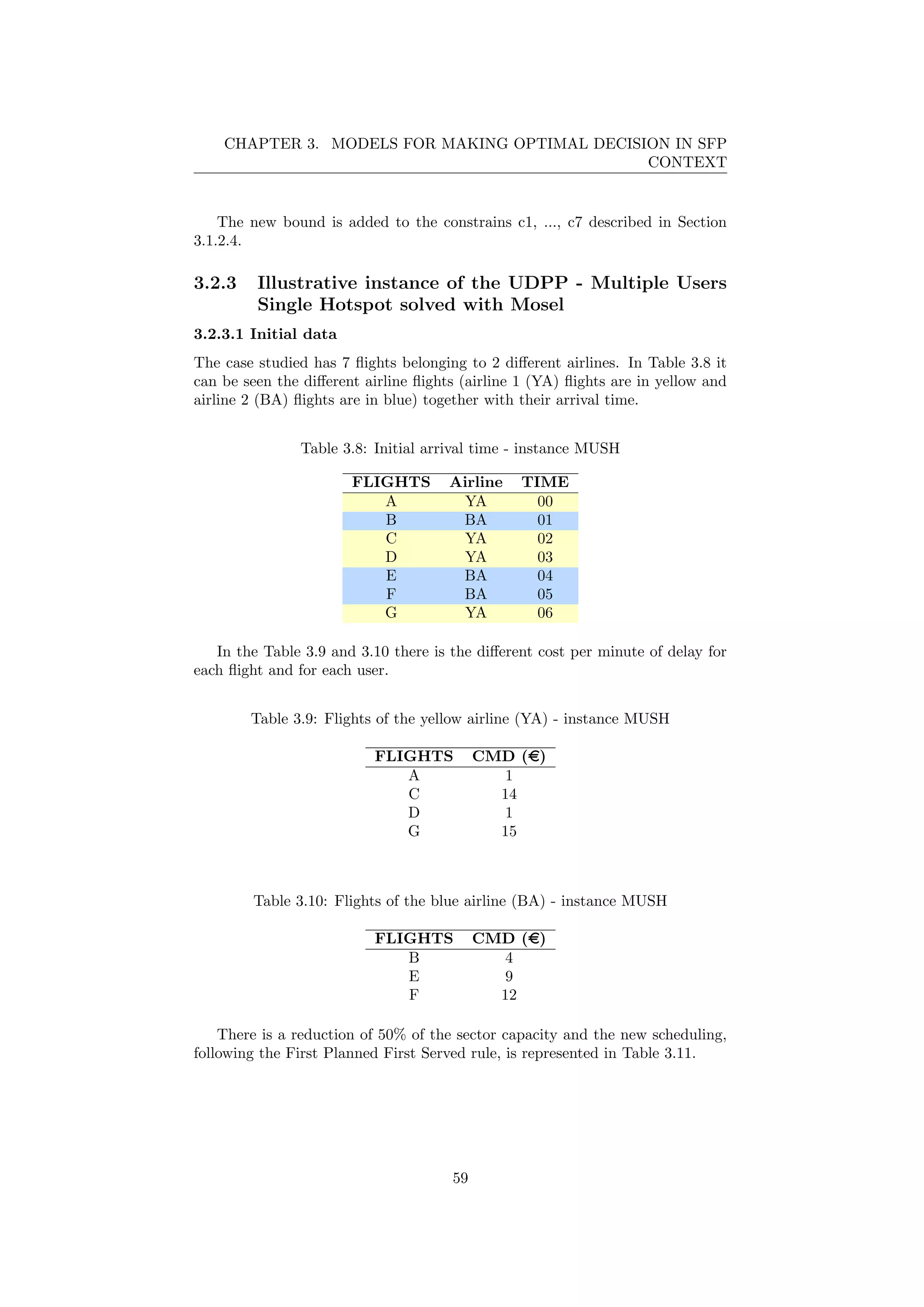
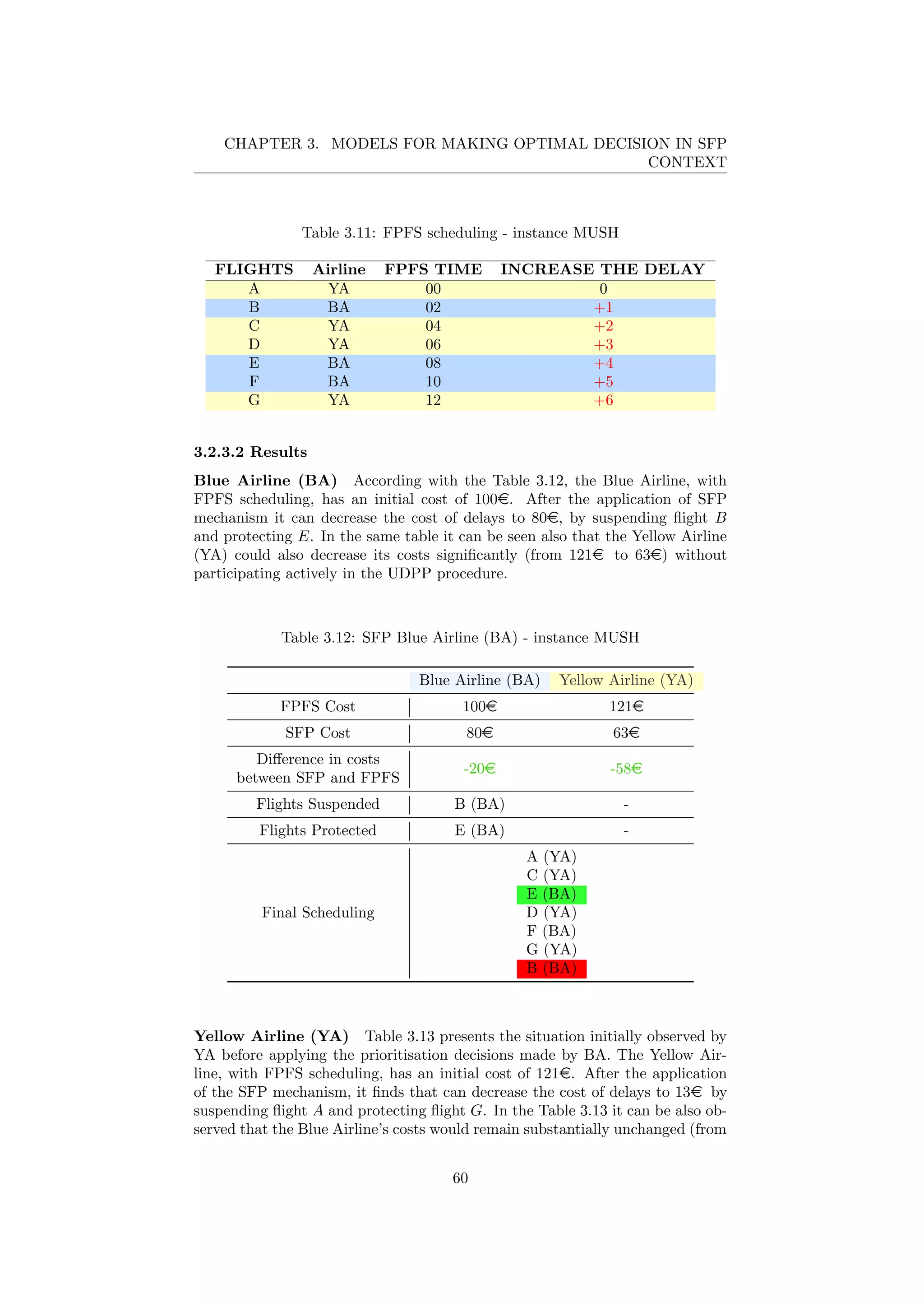
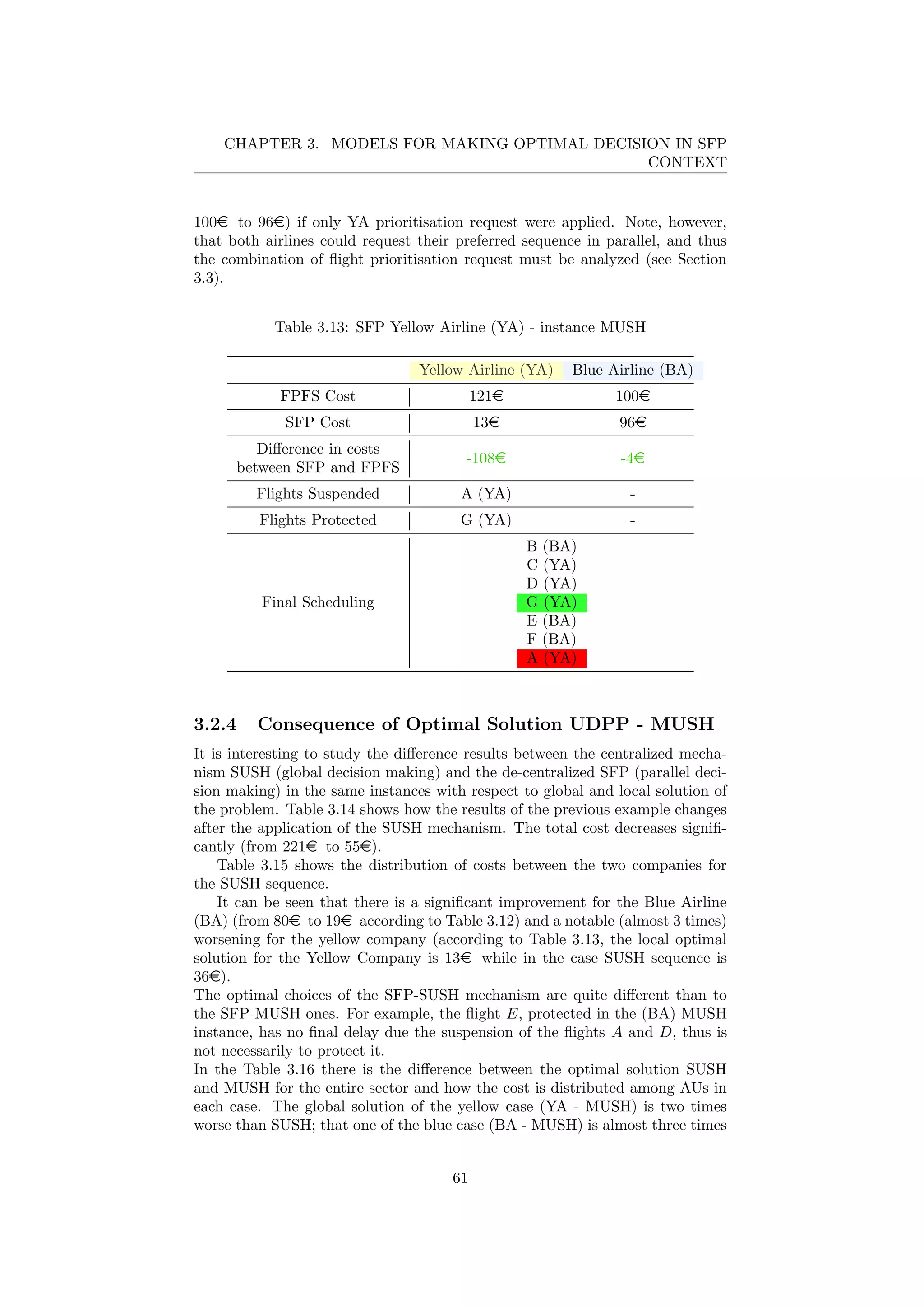
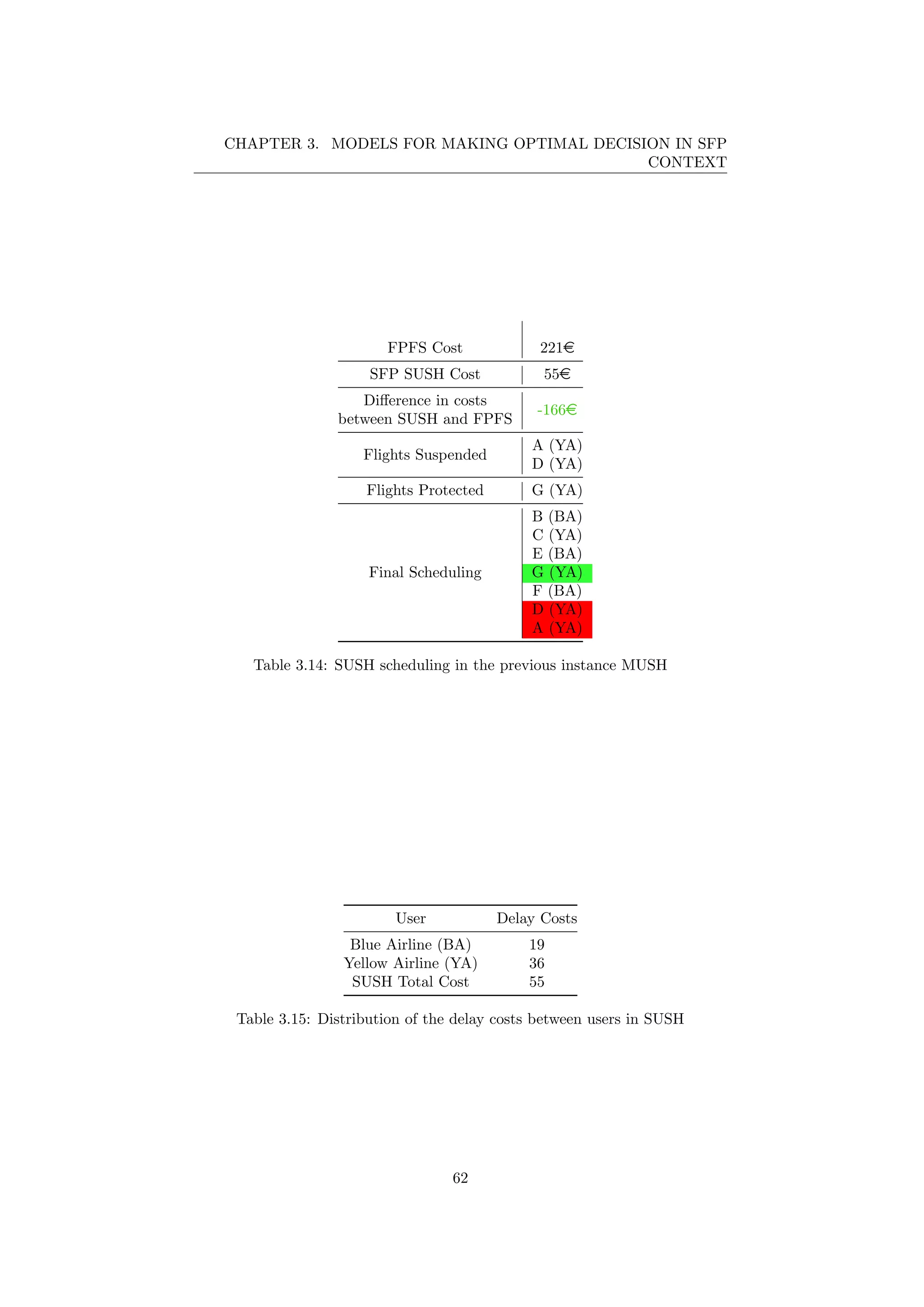
3.2.2.1 Initial data
For MUSH model a new binary vector is required, called MyFlight that repre-
sents which is the set of flights that the user can manage in the sector.
MyFlight =
1 Considered flights
0 Flights of other users
(3.24)
The vector of CMD will be 0 for all flights not considered because the user
does not care about the flights of other airlines. In the real world, airlines do
not usually know the CMD of other companies.
This new vector is complementary to the initial data for SUSH, described in
Section 3.1.2.1.
3.2.2.2 The objective function
The objective function of MUSH model is to minimize the costs for the spe-
cific airline, with no attention to the import of other users (assuming ”selfish
behaviour).
minimize
i in 1...n, j in 1...m
MyFlights(i) · [ x(i, j) · d(i, j) · f(d(i, j)) · CMD(i) ]
(3.25)
f(d(i,j)), as in the SUSH model, is a function related to the delay of the
flights than the slots (see Section 5.1.2).
3.2.2.3 The constraints
There is only one different constraint from the previous model. This new bound-
ary condition puts in a ”normal” status the flights that do not belong to the
selected user.
Constraint c8: ”The flights of other airlines can not be managed”.
∀ i in 1, ..., n
if (MyFlight(i) = 0) ⇒ n(i) = 1
(3.26)
58](https://image.slidesharecdn.com/tesi-160525173017/75/Optimal-decision-making-for-air-traffic-slot-allocation-in-a-Collaborative-Decision-Making-context-59-2048.jpg)
![Chapter 4
Simulator
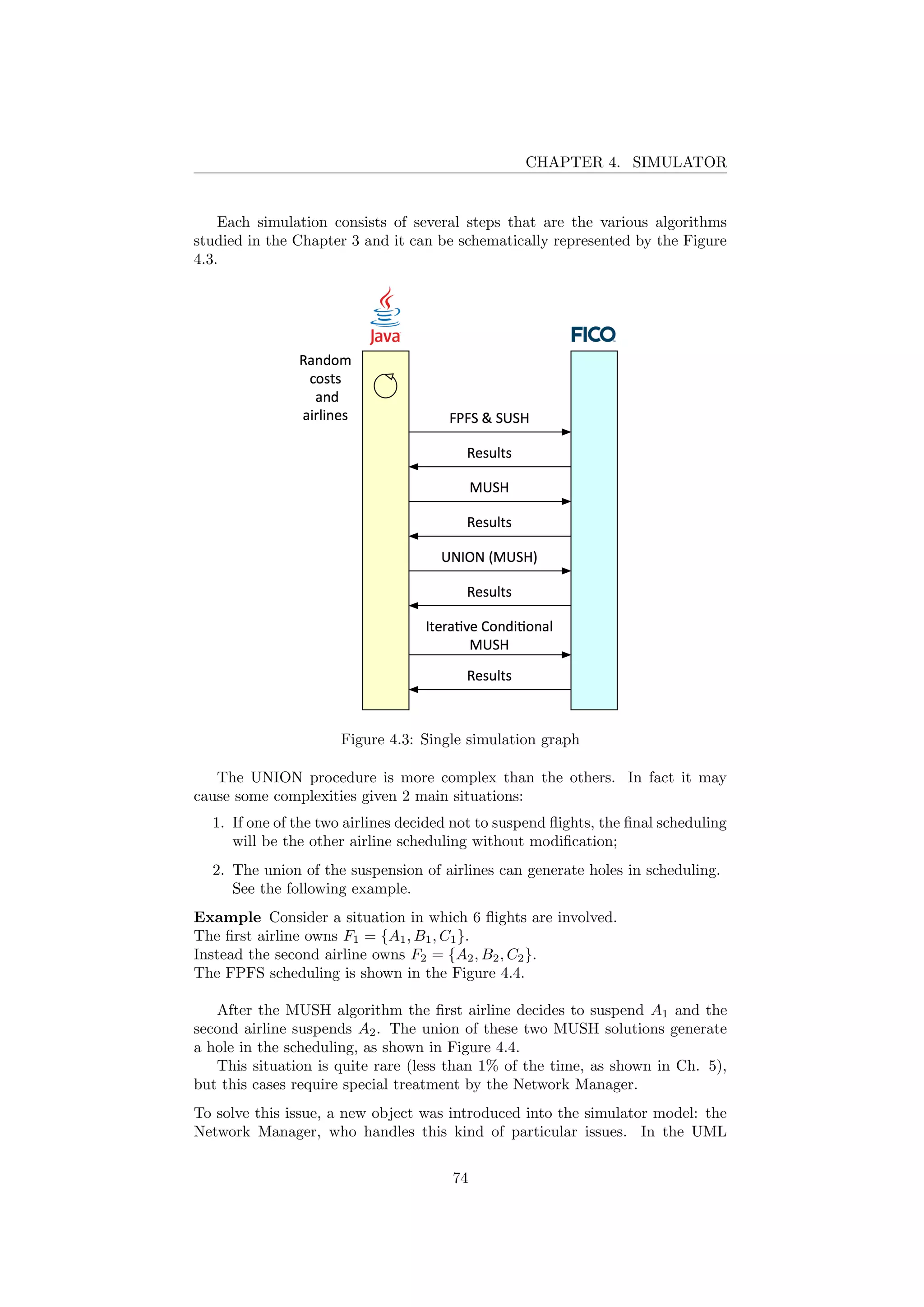
During the last phases of this research, a simulator in JAVA was designed and
implemented to evaluate the different impacts of the various algorithms intro-
duced in Chapter 3.
To program this simulator, the software development platform NetBeans 8.1
has been used[10].
4.1 Concept of the Simulator
The simulator uses the optimization model written in FICO Mosel Xpress to
find the optimal solutions of the instances created and the data is exported in
Microsoft Excel for analysis in an easier and faster way.
Java was considered as the programming language, since it is independent of
the platform and also contains many useful tools and libraries for the purpose
of research.
The core idea of the simulator is to create a connection bridge between JAVA,
FICO Mosel and the final output format: Excel spreadsheet.
Figure 4.1: Concept of the simulator
72](https://image.slidesharecdn.com/tesi-160525173017/75/Optimal-decision-making-for-air-traffic-slot-allocation-in-a-Collaborative-Decision-Making-context-73-2048.jpg)
![CHAPTER 4. SIMULATOR
In order to make the connections between the different layers two different
libraries were used two different libraries:
• Apache POI - the Java API for Microsoft Documents [16], made by The
APACHE Software Foundation;
• XPRD, XPRS, XPRB, XPRM - the JAVA API for FICO Xpress Mosel.
In this software, there are three different layers:
1. the top level: FICO Xpress;
2. the middle level: JAVA;
3. the output level: Apache POI - Excel.
4.2 Design of the Simulator
The simulator recreates hotspots of 15 aircraft that belong to two different air-
lines. The cost of the first minute of delay1
of each flight and of which airline is
each plane are chosen randomly.
After an initial phase of setting (as to set the number of simulations), the
simulator starts to perform by communicating with the various layers as shown
in Figure 4.2.
Figure 4.2: Connection between layers in the simulator
1The CMD is chosen in a range of possibile values due to the studies of cost-delay function,
see Section 5.1.2.
73](https://image.slidesharecdn.com/tesi-160525173017/75/Optimal-decision-making-for-air-traffic-slot-allocation-in-a-Collaborative-Decision-Making-context-74-2048.jpg)
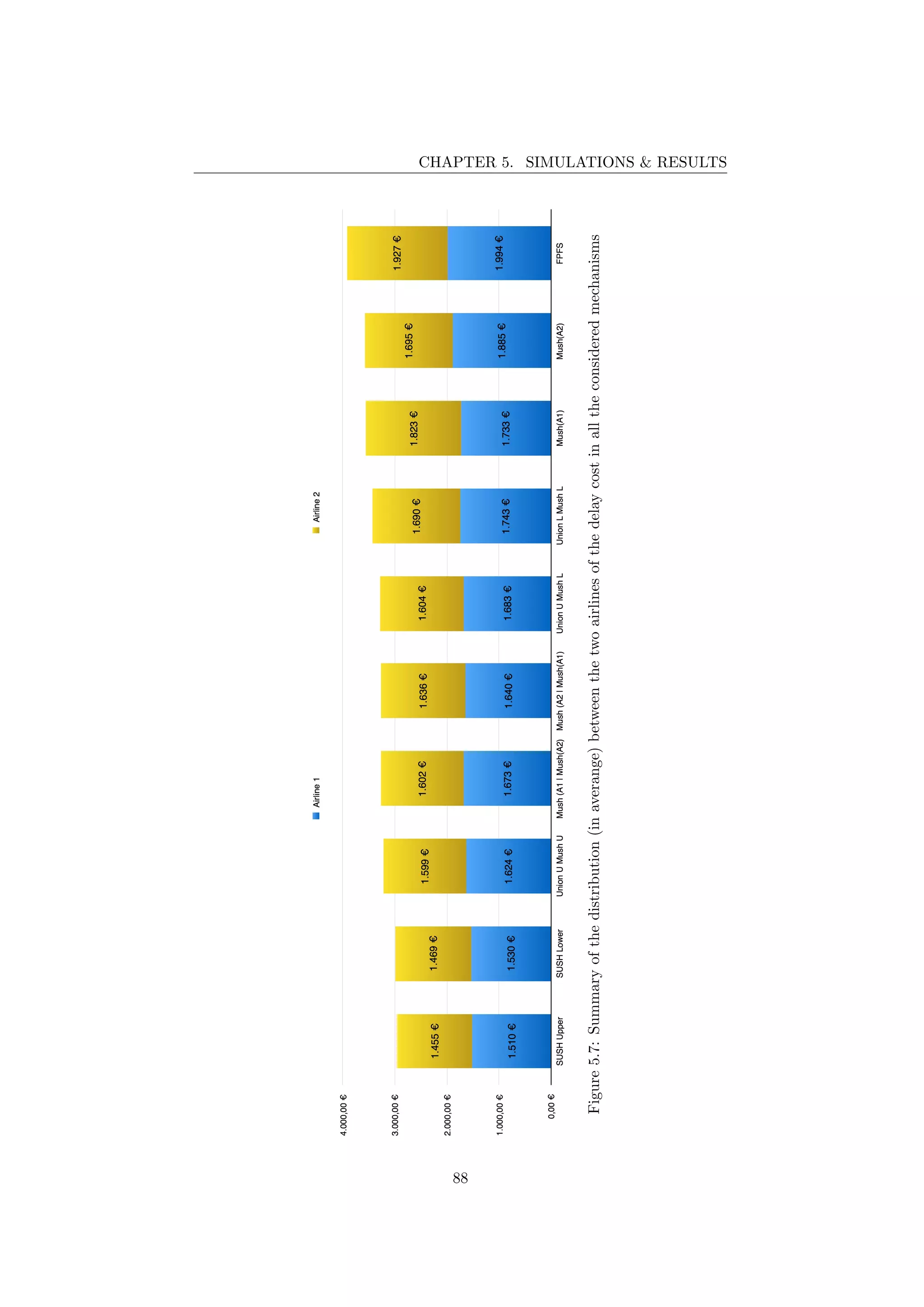
![CHAPTER 5. SIMULATIONS & RESULTS
• no negative delay is allowed (d ≥ 0). It is assumed that the flights cannot
be ready before the time in which the flight was originally planned to
use the slot. In real operations there might be some tolerance. This is a
parameter that can be changed in the model;
• a flight whose initial scheduling time is in the middle of a slot due to a
capacity reduction, it can be associated to that slot with a delay of zero
minutes (no negative delays).
• the granularity of time is in the order of minutes.
• the scheduling of the flights is accurate to the minute;
• the cost of the delay for each plane is calculate precisely (see Section 2.2.1).
In the real world flight operator might have no perfect information about
the actual costs of a flight.
• slots have a constant time size accurate to the minute;
• the demand and capacity are considered to be balanced before the CCS;
• the potential interdependencies between hotspots are not considered;
• each flight has on average 150 passengers;
• the flight delays do not exceed 240 minutes.
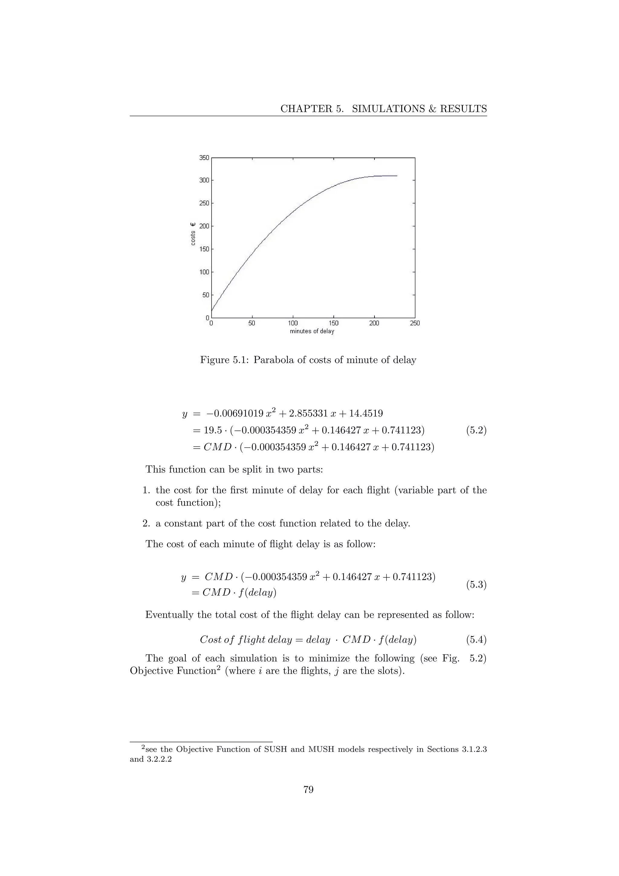
5.1.2 Objective Function parametrization
In Section 2.2.2 it has been introduced the concept of different cost per minute
of delay. Cook, Tanner, Jovanovic and Lawes studied about the cost of delay to
air transport in Europe ([19]) and found a trend of the function similar to that
pointed out in Fig 2.6 (Sec. 2.2.2).
Assuming that each flight has on average 150 passengers, through MATHE-
MATICA Software1
and the data in the Fig. 2.5 (Sec. 2.2.2), it has been found
a mathematical function that has been used to characterized the typical delay
cost structure of flights. The curve that represents (on average) the cost of the
minute delay (not considering delays larger than 240 minutes) is:
y = −0.00691019x2
+ 2.85533x + 14.4519 (5.1)
This function is a parabola and in Fig. 5.1 it can be seen his value between 0
and 240 minutes of delay.
Through the data in Table 2.5 and the assumption about the average num-
ber passengers per flight (150 passengers per flight), it can be argued that the
cost of the first minute of delay (CMD) per flight in a normal cost scenario is
19.5e.
The equation 5.1 can therefore be seen as follows:
1WOLFRAM MATHEMATICA, http://www.wolfram.com/mathematica
78](https://image.slidesharecdn.com/tesi-160525173017/75/Optimal-decision-making-for-air-traffic-slot-allocation-in-a-Collaborative-Decision-Making-context-79-2048.jpg)
![CHAPTER 5. SIMULATIONS & RESULTS
Figure 5.2: Models objective function
5.1.3 Some model implementations issues
As introduced in Section 3.1.2.8, the implementation of the constraint of the
protection (see Section 3.1.2.4 - Constraint c7) has led to the development of
two different models: SFPUpperBound and SFPLowerBound.
The only difference in these models is the implementation of c7, which was
made as follows, respectively:
SFPUpperBound : ”the user is free to allocate the protected flights in any slot
between that one obtained in flight initial allocation (before the reduction of the
sector capacity) and that one resulting by the sequence that follow the FPFS
policy, choosing the best slot for reducing its delay costs”.
This constraint does not ensure that the protected flights are placed in their first
position possible (flights are allocated in the best slot for minimizing the delay
costs which is not necessarily their first possible slot). This is a soft constraint
and the final solution will have slightly lower or equal delay cost than the SFP
optimal solution;
SFPLowerBound : ”the flights protected will be placed only in their initial al-
location slot (before the reduction of the sector capacity) if this is possible, oth-
erwise they will not be protected”. This solution will have the same or slightly
larger cost than the optimal solution.
All simulations were handled with these two models simultaneously in par-
allel in order to evaluate the various differences. The final optimal solution will
be therefore in the range [ SFPUpperBound , SFPLowerBound ].
5.2 Methods for result analysis
The main method used to analyze the simulation results is the linearization of
the solution space within the gap between SUSH and FPFS solutions (i.e., the
best and worst case), as shown in Figure 5.3.
The purpose is to find ”how far” are in percentage the solutions of different
MUSH strategies with respect the best and worst case (see Section 5.4 where
the discussion about the need and interest of such analysis can be found), with
respect the total delay cost in a sector (total delay cost), but also for each AU
80](https://image.slidesharecdn.com/tesi-160525173017/75/Optimal-decision-making-for-air-traffic-slot-allocation-in-a-Collaborative-Decision-Making-context-81-2048.jpg)

![APPENDIX A - ORDERS
OF COMPLEXITY
During this research it has been treated several times the orders of complexity
in the algorithms found. In this appendix, it will be explained how that kind of
orders are structured and it will be introduced the Big O notation [15].
Big O Notation
Big O notation is a mathematical notation that describes the limiting behavior
of a function when the argument tends towards a particular value or infinity. It
is how fast a function grows or declines. It is a member of a family of notations
invented by Edmund Landau and Paul Bachmann (indeed it is called Bachmann-
Landau notation (or asymptotic notation)). The letter O is used because the
rate of growth of a function is called order.
Example To describe the complexity of an algorithm it is defined a function
which evaluates the total number of steps (or the amount of time) given an
initial problem of size n.
E.g. this value is T(n) = 15n3
− 6n2
+ 3n + 2.
The constants and the slower growing terms will be ignored and it can be said
that T(n) grows at the order of n3
and write: T(n) = O(n3
).
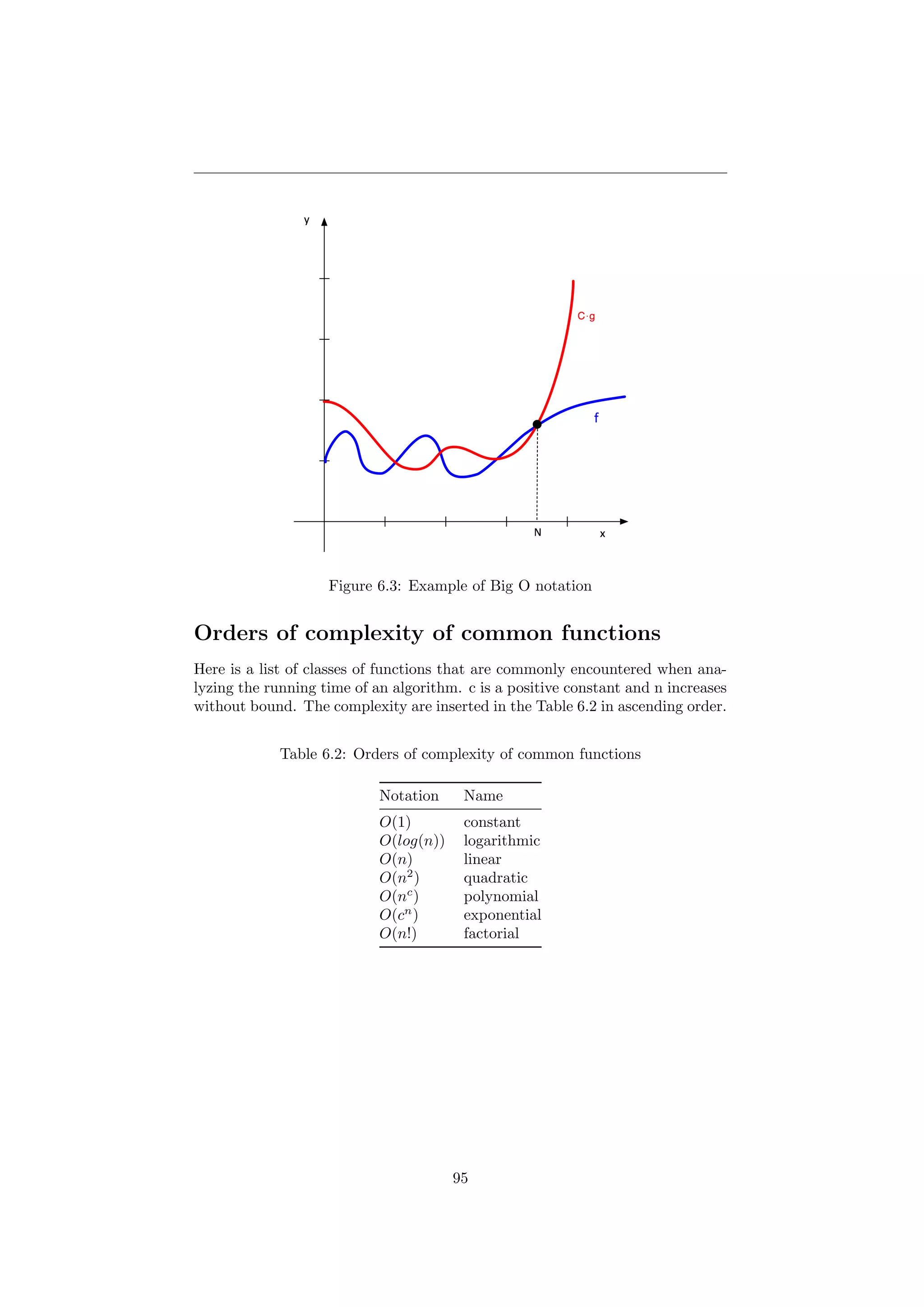
For the formal definition, suppose f(x) and g(x) are two functions defined
on some subset of the real numbers.
f(x) = O(g(x)) for x → ∞ (6.1)
if and only if there exist constants N and C such that
|f(x)| ≤ C|g(x)| for all x > N (6.2)
f does not grow faster than g.
94](https://image.slidesharecdn.com/tesi-160525173017/75/Optimal-decision-making-for-air-traffic-slot-allocation-in-a-Collaborative-Decision-Making-context-95-2048.jpg)
![Bibliography
[1] Eurostat, Passenger transport statistics, data from January 2016.
[2] EUROCONTROL, Seven-Year Forecast, February 2015.
[3] SESAR, European ATM Master Plan, 2015.
[4] T. Vossen, M. Ball, Optimization and Mediated Bartering Models for
Ground Delay Programs, Naval Research Logistics 51, pp. 75-90, 2006
[5] L. Castelli, R. Pesenti, A. Ranieri, The design of a market mechanism to
allocate Air Traffic Flow Management slots, Transportation research part
C: Emerging technologies 19 (5), 931-943, 2011.
[6] europa.eu Welcome to the SESAR project, 2015.
[7] EUROCONTROL Lexicon, UDPP, www.eurocontrol.int/lexicon/lexicon/en/index.php/UDPP.
[8] S. Ruiz, Strategic Trajectory De-confliction to Enable Seamless Aircraft
Conflict Management, Ph.D Thesis, 2013
[9] SESAR Joint Undertaking. http://www.sesarju.eu.
[10] NETBEANS, https://netbeans.org
[11] R. Hoffman, Integer Programming Models for Ground-Holding in Air Traf-
fic Flow Management, Ph.D Thesis, 1997
[12] FICO Xpress Optimisation Suite, www.fico.com
[13] D. G. Luenberger, Y. Ye, Linear and Nonlinear Programming, Third Edi-
tion, Springer, 2008
[14] EUROCONTROL, European Network Operations Plan 2015 - 2019, 2015
[15] MIT - Introduction to Computer Science and Programming - Lecture 8:
Efficiency and Order of Growth
[16] Apache POI - the Java API for Microsoft Documents,
https://poi.apache.org
[17] C. Demetrescu, I. Finocchi, Algoritmi e strutture dati, McGraw-Hill, 2008
[18] FICOT M
Xpress Optimization Suite, MIP formulations and linearizations,
2009
97](https://image.slidesharecdn.com/tesi-160525173017/75/Optimal-decision-making-for-air-traffic-slot-allocation-in-a-Collaborative-Decision-Making-context-98-2048.jpg)
![[19] A. Cook, G. Tanner, R. Jovanovic, A. Lawes, The cost of delay to air
transport in Europe - quantification and management, 13th Air Transport
Research Society (ATRS) World Conference, 27-30 June 2009, Abu Dhabi,
United Arab Emirates, Paper No. 107
[20] S. Martello, Fondamenti di ricerca operativa, progetto Leonardo, 2006
[21] P. Serafini, Ricerca Operativa, Springer, 2008
[22] SESAR, UDPP Credits feasibility report, 2015
[23] Computing in Science and Engineering, volume 2, no. 1, 2000
[24] M. Ball, C. Bamhart, G. Nemhauser, A. Odoni, Air Transportation: Ir-
regular Operations and Control, in G. Laport and C. Barnhart, editors,
Handbooks in Operations Research & Management Science: Transporta-
tion, Handbooks in Operations Research and Management Science. North
Holland (8 Dec 2006), 2006.
[25] L. Castelli, R. Pesenti, A. Ranieri, Allocating Air Traffic Flow Management
Slots, International journal of revenue management 6 (1-2), 28-44, 2011
98](https://image.slidesharecdn.com/tesi-160525173017/75/Optimal-decision-making-for-air-traffic-slot-allocation-in-a-Collaborative-Decision-Making-context-99-2048.jpg)