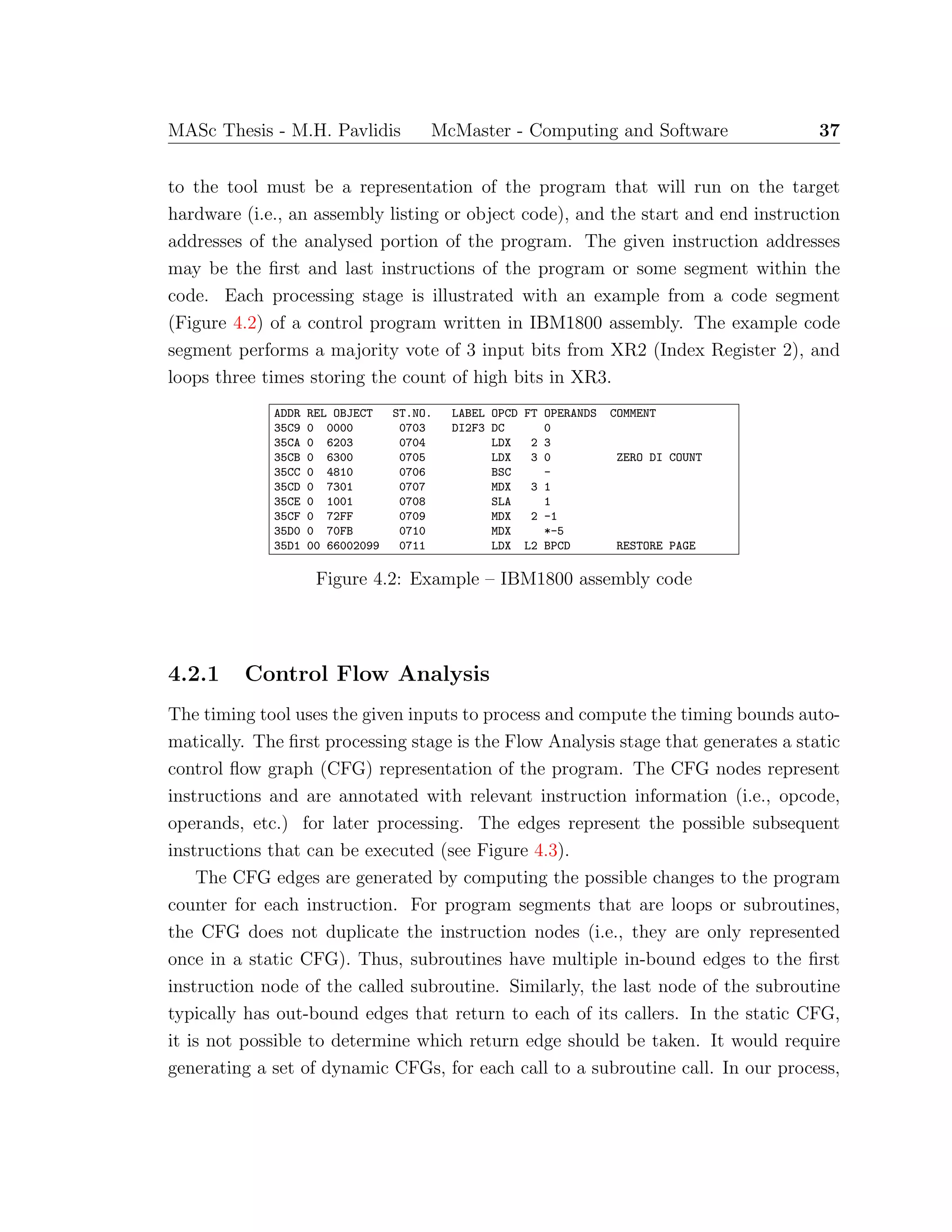
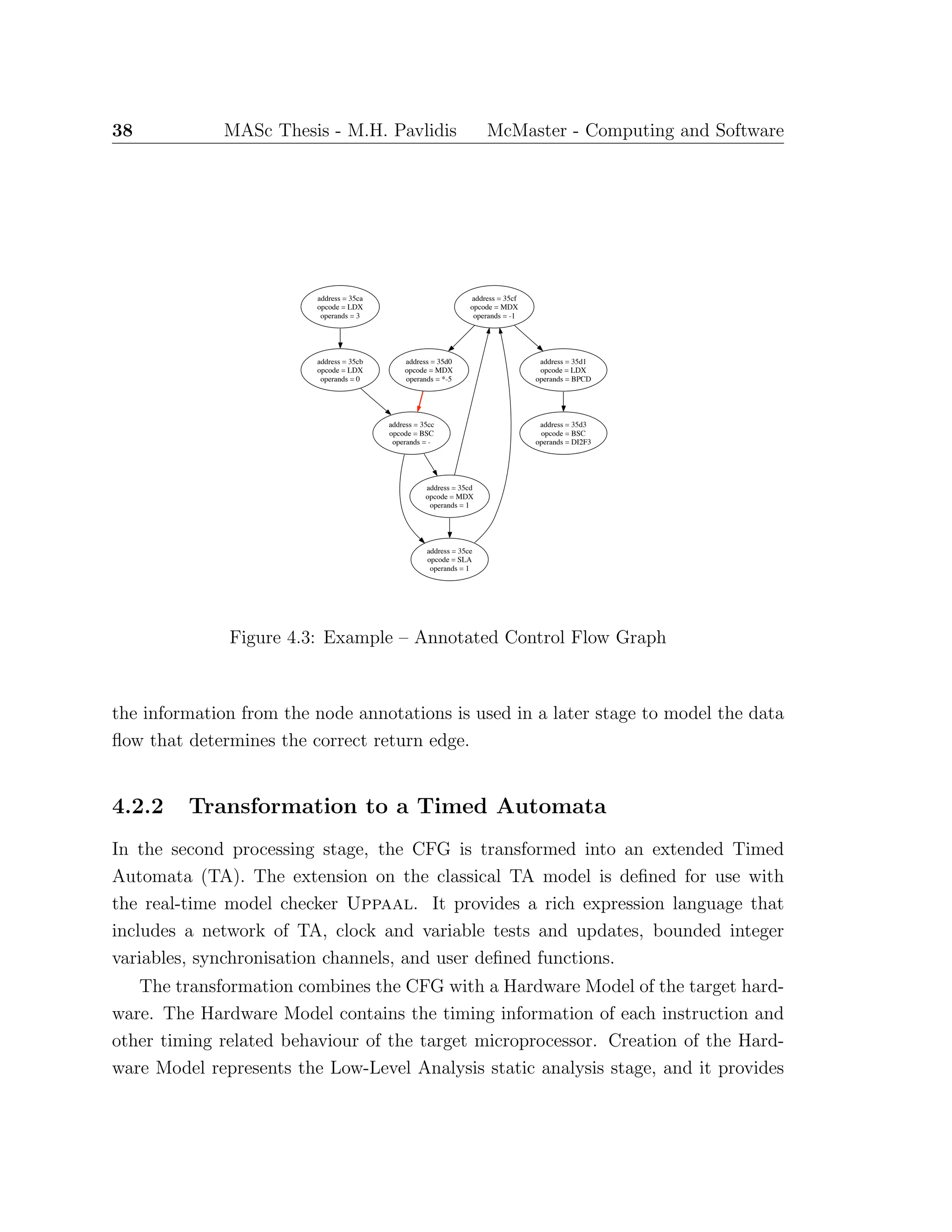
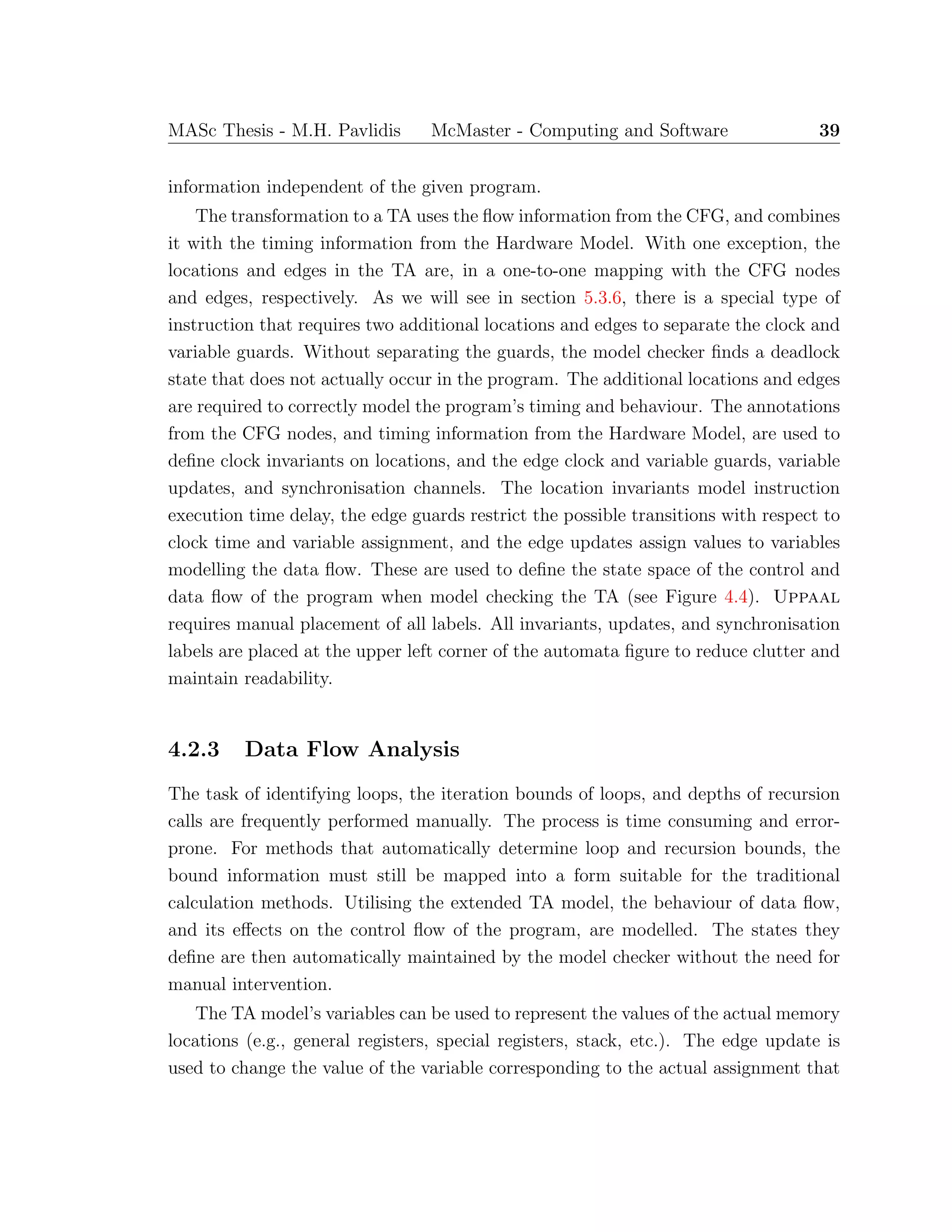
This thesis proposes an automated method for obtaining tight best-case and worst-case timing bounds on unstructured assembly code without manual annotation. A control flow graph is generated from assembly code and transformed into a timed automata model. Instruction times are modeled and the processor state is tracked with variables. Model checking is used to extract shortest and longest paths, yielding best-case and worst-case execution times. The method is demonstrated on examples for the PIC and IBM1800 microcontrollers.


![Chapter 1
Introduction
Why do we need the timing bounds of an embedded real-time program?
Embedded real-time systems are used to control many tasks in the physical world
that were not previously controlled with computers. These include safety-critical
tasks such as the control of nuclear power generating stations, aerospace and auto-
motive vehicles, and telecommunication systems among others. A commonality of
these tasks is that they are increasingly being implemented as software programs
controlling embedded real-time systems. A system failure due to a missed timing
deadline may result in catastrophic loss of human and/or economic resources. More-
over, on a volume basis, nearly all processors (up to 98%) manufactured are used in
embedded systems[41]. Therefore, a great deal of research effort has gone into devel-
oping methods to verify that these systems meet functional requirements to ensure
correct operation.
More recently, research on determining timing bounds of embedded systems has
been pursued. The timing bounds include both the Worse Case Execution Time
(WCET) and Best Case Execution Time (BCET) of the system. The timing bounds
are used in the validation of the timing requirements of the systems. The timing
of the execution of a real-time program is critical in determining if the functional
requirements are met, because control of physical systems require that decisions must
made by some hard real-time limit. Furthermore, a large variance in timing of control
decisions may make the physical system unstable. Timing bounds are also used in
schedulability analysis of the system, and determining the capabilities (and cost) of
1](https://image.slidesharecdn.com/1cc5036e-53e1-4bf9-87fe-9bea3c729be7-150414001600-conversion-gate01/75/thesis-hyperref-15-2048.jpg)
![MASc Thesis - M.H. Pavlidis McMaster - Computing and Software 3
Semantic Analysis Library
Graph Generation Tools & Library
Timing Analysis Tool
Semantic Analysis Tools
Requirements Repository
Graph Analysis Tools
Assembly Representation
Library & Emulators
Requirements V&V Tools
(Scenario Analysis, Testing, etc.)
Functionality Analysis &
Design Recovery Tools
Figure 1.1: Reverse Engineering Tool Suite Uses Hierarchy
worst-case execution times are required. Finally, it was necessary to address and
overcome limitations of a previous timing analysis tool by fully automating the timing
analysis process.
1.1.2 Timing Analysis Difficulties
The conceptual use of WCET in scheduling algorithms for hard real-time systems
has long been studied [27], but determining the actual precise execution time bounds
of real-time programs is difficult, error-prone, and time consuming. More recently,
research has focused on determining the WCET estimate that is a safe overestimate
using static analysis of the program source or object code.
Static timing analysis methods have reduced much of the time and effort required
to obtain timing bound results, but they do not entirely eliminate the human-in-the-
loop required to add annotations for control flow. The required annotations include
determining loop iteration bounds, branching flow and infeasible paths, and behaviour
due to function calls and recursion. Some methods to automatically determine pro-
gram behaviour have been developed [13], but these are restricted to special cases of](https://image.slidesharecdn.com/1cc5036e-53e1-4bf9-87fe-9bea3c729be7-150414001600-conversion-gate01/75/thesis-hyperref-17-2048.jpg)
![4 MASc Thesis - M.H. Pavlidis McMaster - Computing and Software
structured code and/or require high-level source code (recall the constraint of reverse
engineering assembly code).
1.1.3 Timing Bound Uses
To answer the opening question why we need to determine the timing bounds of real-
time programs?, we look at the uses of the timing bounds. First is the need to
determine timing bounds that satisfy functional timing requirements and timing tol-
erances in reverse engineering safety-critical real-time programs to high-level require-
ments. Moreover, determining the timing bounds of an implementation can be used
in the forward development process to validate a program implementation against
functional timing requirements, and verify that the jitter is acceptable for the spec-
ified timing tolerances [43]. Finally, other uses for timing bounds include selection
of sampling frequency, data rates, schedulability, hardware (i.e., processor) selection,
and complier optimisation.
1.2 Related Work
In this section, the work directly related to the development of the Symbolic Timing
Analysis of Real-Time Systems (STARTS) tool suite is presented. It includes work
previously completed for the Reverse Engineering project, and other tools used in its
implementation.
1.2.1 Timing Analysis Tool
A WCET Analysis Tool (WAT) was developed by Sun [36]. The tool was developed
to be the Timing Analysis Tool (TAT) component of the Reverse Engineering Tool
Suite. The interactive tool consists of a path-based WCET calculation. It partially
automates analysis, but it still requires intensive manual annotation to identify loops
and determine their bounds, and to mark infeasible paths. Further, the traces are
generated as sequential textual output.
These limitations of the WAT motivated development of a tool that automates
the process to eliminate time consuming and error-prone manual annotations. It also](https://image.slidesharecdn.com/1cc5036e-53e1-4bf9-87fe-9bea3c729be7-150414001600-conversion-gate01/75/thesis-hyperref-18-2048.jpg)
![MASc Thesis - M.H. Pavlidis McMaster - Computing and Software 5
identified the need for a graphical visualisation of the traces as an aid in comprehen-
sion for the reverse engineering efforts. Additionally, a tool that finds both BCET
and WCET is preferred to one that only computes the latter. The development of
the WAT provides a methodology for obtaining possible execution traces and insight
into troublesome IBM1800 instructions that complicate feasible path determination.
The feasible paths are found by pruning the infeasible edges from the output of a
Control Flow Graph tool.
1.2.2 Control Flow Graph Tool
Everets [14] implemented a tool for generating a static control flow graph (CFG) rep-
resenting an approximation of the possible execution paths of the BPC code. The tool,
Lst2Gxl, is a part of one of the lowest-level components, the Graph Analysis Tool,
of the Reverse Engineering Toolset. Lst2Gxl uses the complier generated code listing
(LST) file to create a CFG with each instruction represented as a node in the graph.
The graph nodes include additional annotations that contain relevant information
from the assembly code that can be further used to determine the feasible dynamic
execution paths. Figure 1.2 is an example of a CFG generated from a code segment of
the IBM1800 assembly code. The CFG is represented in Graph eXchange Language
(GXL) [19], an Extensible Markup Language (XML) sub-language designed to be a
standard exchange format for graphs. The GXL-based CFG can be processed by Ex-
tensible Stylesheet Language Transformation (XSLT) [47], an XML-based language
used for the transformation of XML documents, to another XML-based document.
For example in Section 6.2.4, an XSLT specification is defined to transform a CFG
in GXL to an XML-based timed automata model used by Uppaal.
1.2.3 UPPAAL
Uppaal is a graphical tool for modelling, simulation and verification of real-time
systems [42], depicted in Figure 1.3. It is appropriate for systems that can be modeled
as a collection of non-deterministic processes with finite control structure and real-
valued clocks (i.e., timed automata), communicating through channels and/or shared
data structures.
Typical application areas include real-time controllers, communication protocols,](https://image.slidesharecdn.com/1cc5036e-53e1-4bf9-87fe-9bea3c729be7-150414001600-conversion-gate01/75/thesis-hyperref-19-2048.jpg)

![MASc Thesis - M.H. Pavlidis McMaster - Computing and Software 7
Figure 1.3: Uppaal 3.6 Screenshot - Modeling Editor
and other systems in which timing aspects are critical. Uppaal is a joint develop-
ment between real-time system researchers at Uppsala University, in Sweden, and
Aalborg University, in Denmark. It provides a model checking engine to verify safety
and bounded liveness properties expressed as reachability queries [24, 3]. It was ini-
tially released in 1995, and it continues to be actively developed and supported on
MS Windows, Linux, and Mac OS X platforms. Throughout the years, many no-
table improvements have been made to Uppaal, including efficient data structures
and algorithms, symmetry reduction, and symbolic representations that dramatically
reduce computation time and memory space use in light of possibly enormous state
space explosion.
The most recent stable release, version 4.0.1 (as of June 2006), includes a stan-
dalone verification engine, fastest trace generation (for BCET)1
, XML-based TA
model, process priorities, progress measures, bounded integer ranges, meta variables,
and user-defined functions. These features permit the modeling of microprocessor ar-
chitecture and instruction execution used to perform timing analysis by the method
proposed in this thesis.
1
The slowest trace generation is currently possible in an unreleased prototype version of Uppaal.](https://image.slidesharecdn.com/1cc5036e-53e1-4bf9-87fe-9bea3c729be7-150414001600-conversion-gate01/75/thesis-hyperref-21-2048.jpg)

![14 MASc Thesis - M.H. Pavlidis McMaster - Computing and Software
2.2.2 Timed Automata
The theory of timed automata was initially developed by Alur and Dill [5], as an
extention of finite-state B¨uchi automata with clock variables. A timed automaton is
structured as a directed graph with nodes representing locations and edges represent-
ing transitions.
Constraints on the clocks are used to restrict the behaviour of the automaton and
enforce progress properties. Clock constraints on locations, called invariant condi-
tions, force a transition when a clock value would violate the clock invariant. The
transition (if one exists) is required because states where the clock invariant is violated
are considered infeasible.
Transitions of the automaton have clock constraints guarding the transition edge,
called triggering conditions, restricting when a transition can be taken based on the
clock guard. Transitions include clock resets, where some clock variables are reset to
zero when the transition is taken.
Definition 2.4 A Timed Automaton is a tuple,
A = (L, C, l0, E, I),
where L is a finite set of locations, C is a finite set of non-negative real-valued clocks,
l0 ∈ L is an initial location, E ⊆ L×B(C)×2C
×L is a set of edges labelled by guards
and a set of clocks to be reset, and I : L → B(C) assigns location invariants to clocks,
where B(C) = x, c, ∼ | x ∈ C ∧ c ∈ N ∧ ∼∈ {<, ≤, ==, ≥, >} : x ∼ c is the set of
guards on clocks.
Bengtsson et al. [8] provide an extension of the classical theory of timed automata
to ease the task of modelling with a more expressive language. The extension adds
more general data type variables (i.e., boolean, integer), in an attempt to make the
modelling language closer to real-time high-level programming languages.
Definition 2.5 An Extended Timed Automaton is a tuple,
Ae = (L, C, V, A, l0, E, I),
where L is a finite set of locations, C is a finite set of non-negative real-valued clocks,
V is a set of finite data variables. A is the set of synchronising actions where](https://image.slidesharecdn.com/1cc5036e-53e1-4bf9-87fe-9bea3c729be7-150414001600-conversion-gate01/75/thesis-hyperref-28-2048.jpg)

![18 MASc Thesis - M.H. Pavlidis McMaster - Computing and Software
Hardware measurement methods have minimal intrusiveness on the software be-
ing measured because probing does not affect execution time or order of execution.
However, the methods can only be used on a system when the hardware setup per-
mits the connection of the analysing probes. An example of a scenario that does not
permit the use of such tools would be an embedded safety-critical system, where it
is not be safe to connect probes to hardware or run test cases they may result in a
system failure.
Oscilloscope measurements only provide results from externally visible signals,
and cannot determine the internal state of the processor or executing program. How-
ever, the granularity of logic analysers is at the machine instruction level. For both
methods, the measurements of numerous test executions are logged, and the changes
of signals over time are analysed to determine the timing results. Although these
methods provide the smallest timing resolutions, as with all of the dynamic WCET
methods, it cannot typically guarantee safe timing bounds because in general test
cases cannot be exhaustive. The latter is also true for the software measurement
techniques described below.
3.1.2 Software Measurements
Software measurements involve adding instrumentation points into the source code of
the program or around the program. An example of software measurement methods
are function profiling tools (e.g., gprof() [17]) that measure the execution profile of
called subroutines, providing a call graph and associated execution time. Another
is using instrumentation points that drive output pins that can be measured with
hardware to determine the execution time.
Unfortunately, adding instrumentation code into a real-time program changes the
timing, execution path and, for complex processors with cache and pipelines, proces-
sor dynamics, of the program proper. It results in an overestimation for the timing
bounds. The impact on the WCET bound is an overestimated result, that is more
safe. The impact on the BCET bound is far more critical to the analysis of response
jitter, since the overestimation can push the BCET bound into to the right of the
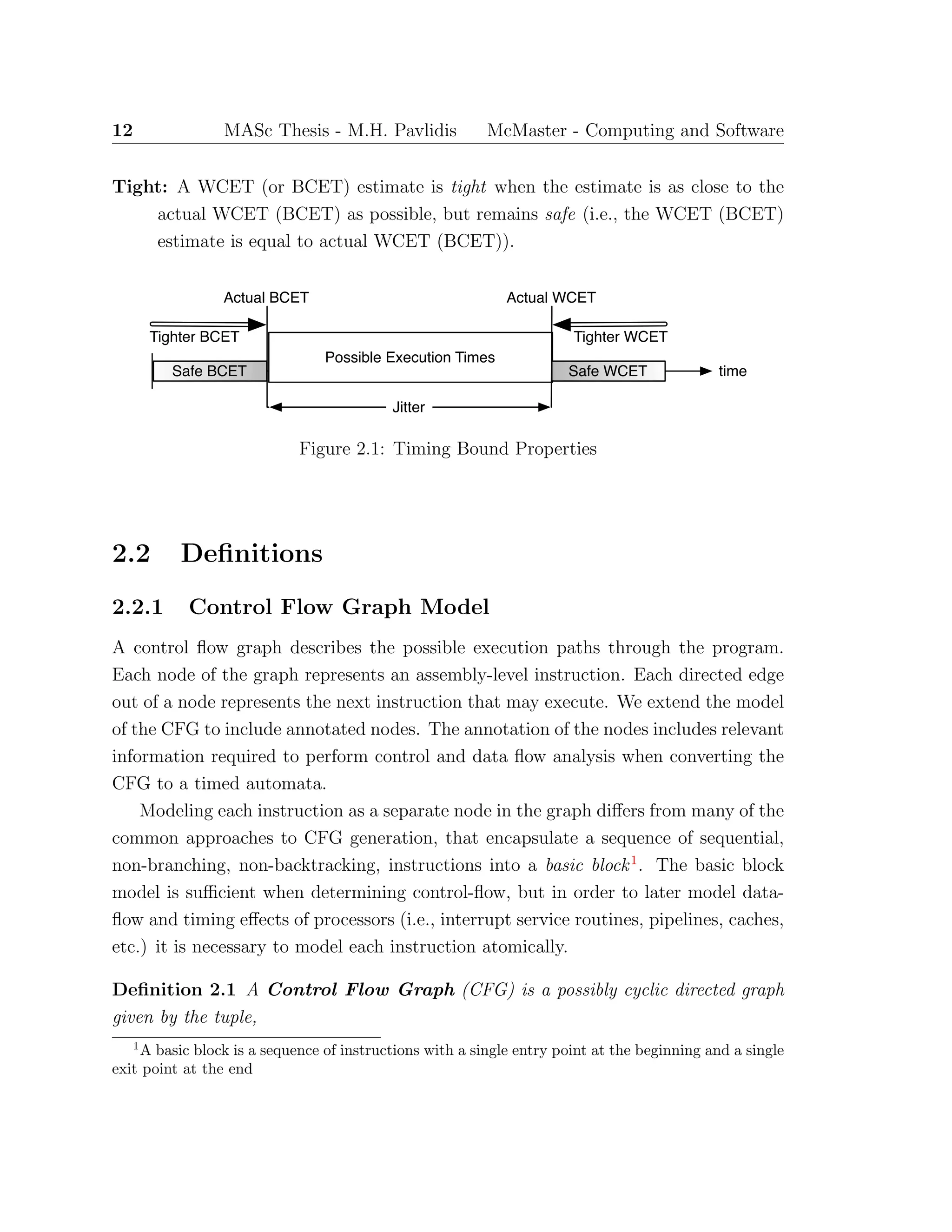
safe BCET time region, as illustrated in Figure 2.1, leading to an underestimated
response jitter.](https://image.slidesharecdn.com/1cc5036e-53e1-4bf9-87fe-9bea3c729be7-150414001600-conversion-gate01/75/thesis-hyperref-32-2048.jpg)
![MASc Thesis - M.H. Pavlidis McMaster - Computing and Software 19
Software measurements that do not add instrumentation points in the code require
operating system or emulator support to obtain the start and end times of execution.
The former has a high granularity (i.e., program level) and high timing resolution
that is dependent on the operating platform (i.e., UNIX time() command). Emulation
provides instruction level granularity, low timing resolution, and can provide execution
traces, but development of an emulator can be costly and time consuming.
3.1.3 Dynamic Timing Analysis Feasibility
Despite its common use in industry, it is very difficult for dynamic timing analysis
to ensure safe timing bound results. The methods yield timing bounds that are
within the range of possible execution time (Figure 2.1). The initial state and input
selection of test cases strives to push the results outward toward the actual bounds.
For safety-critical real-time systems, if system response is too fast or too slow it
can cause the system to enter a state that is unstable and uncontrollable, resulting in
possible catastrophic failure. Thus dynamic timing analysis techniques do not provide
a feasible solution to our problem with its previously stated set of constraints. The
requirement to obtain safe timing bounds motivated the investigation of static timing
analysis methods. More recently, dynamic measurement techniques have been used
to enhance static analysis in [44] for high-end processors that cannot be effectively
analysed due to computational complexity. We note that to avoid these complexities
and because of market factors, we limit our analysis to the class of processor that are
low-end, for which static timing analysis is feasible.
3.2 Static Timing Analysis
Static timing analysis involves the use of analytical methods to determine timing
bounds from program code (high-, assembly-, or object-level) without executing the
code. Each stage of static timing analysis provides information about a program
and its execution architecture used to obtain a safe and tight (as possible) WCET.
This section outlines the three stages of static WCET analysis, commonly presented in
literature, and presents some timing analysis tools that provide static timing analysis.](https://image.slidesharecdn.com/1cc5036e-53e1-4bf9-87fe-9bea3c729be7-150414001600-conversion-gate01/75/thesis-hyperref-33-2048.jpg)
![20 MASc Thesis - M.H. Pavlidis McMaster - Computing and Software
3.2.1 Flow Analysis
The first stage of static timing analysis involves determining possible sequences of
instruction execution of the program. This includes sequential blocks of instructions,
branching and conditional branching instructions, and number of loop iterations. For
the latter, the common approaches require manual annotation of loop iterations. This
thesis presents a method that does not require manually determining loop bounds a
priori. The flow analysis is represented by a CFG, where instructions are represented
by nodes and the execution path is determined by the directed edges.
In cases where source code is available, the flow analysis stage may also determine
called functions and recursions. Based on the constraints of the reverse engineering
problem, high-level source code will not be considered in the implementation of the
timing analysis tool, and it is only mentioned for completeness.
Flow analysis must determine a safe execution path approximation, that includes
all feasible paths with as few infeasible paths as possible. In the method proposed
in this thesis, Low-level Analysis (Section 3.2.2) of the architecture yields conditions
on edges that prevent inclusion of infeasible paths in the timing bound calculation.
Calculation methods that do not perform partial data flow simulation do not maintain
enough of the state information to eliminate infeasible paths from the calculation of
the timing bounds. This results in time bounds that are less tight. The task of flow
analysis is decomposed into three steps: Extraction, Representation, and Calculation
conversion.
Extraction of flow information for assembly-level code involves the identification
of all possible paths for each instruction based on the operational semantics of the
architecture, typically defined informally in the technical manuals of the target pro-
cessor.
Once flow information is extracted, it is necessary to introduce notation to rep-
resent it. The representation of flow analysis may take the form of some type of
graph [34, 37, 45] or tree [33, 10], source code annotation [22], or by defining a lan-
guage to describe the possible paths through the program [31, 21]. Together with
flow information, loop identification and loop iteration bounds are added to the flow
representation. Commonly, loop information is annotated manually. Since manual
annotation is prone to error and tedious, there have been some developments in au-](https://image.slidesharecdn.com/1cc5036e-53e1-4bf9-87fe-9bea3c729be7-150414001600-conversion-gate01/75/thesis-hyperref-34-2048.jpg)
![MASc Thesis - M.H. Pavlidis McMaster - Computing and Software 21
tomatically identifying loops and related iteration bounds at assembly-level code for
some classes of well-structured loops [18].
The choice of representation may negatively impact the capabilities of the related
Calculation method (Section 3.3) to find safe and tight timing bounds. In the final
step, Calculation conversion, the flow information is mapped to a form that is a
feasible input for the chosen method of computing the bounds. In addition to flow
information to perform the calculation, the execution time of the underlying hardware
architecture must be determined by low-level analysis.
3.2.2 Low-Level Analysis
The precise execution time of each instruction is determined at the low-level analysis
stage. The target architecture instruction set defines each atomic action the processor
performs, and how long each action takes. The execution time of each instruction
is impacted by the complexity of the architecture. Microprocessor designers add
physical complexity to increase instruction throughput with pipelined and out-of-order
execution, and to decrease memory access delays with cache. We leave investigation
of these types of processors to future work as they are outside of the scope of our
problem definition.
Logical complexity is added the the hardware architecture with interpreted in-
structions, where the operator mnemonic (or opcode) alone does not determine the
action of the instruction. Further, for some complex architectures (i.e., CISC-based
processors like the Intel x86 line) instructions are interpreted into a set of micro-
instructions encapsulated in the hardware and hidden from the instruction set. More
logical complexity of the instruction set requires interpreting the instruction opera-
tor, flag bits, and operands. This is done to understand the action performed by the
processor for each instruction format, and accordingly the precise execution time.
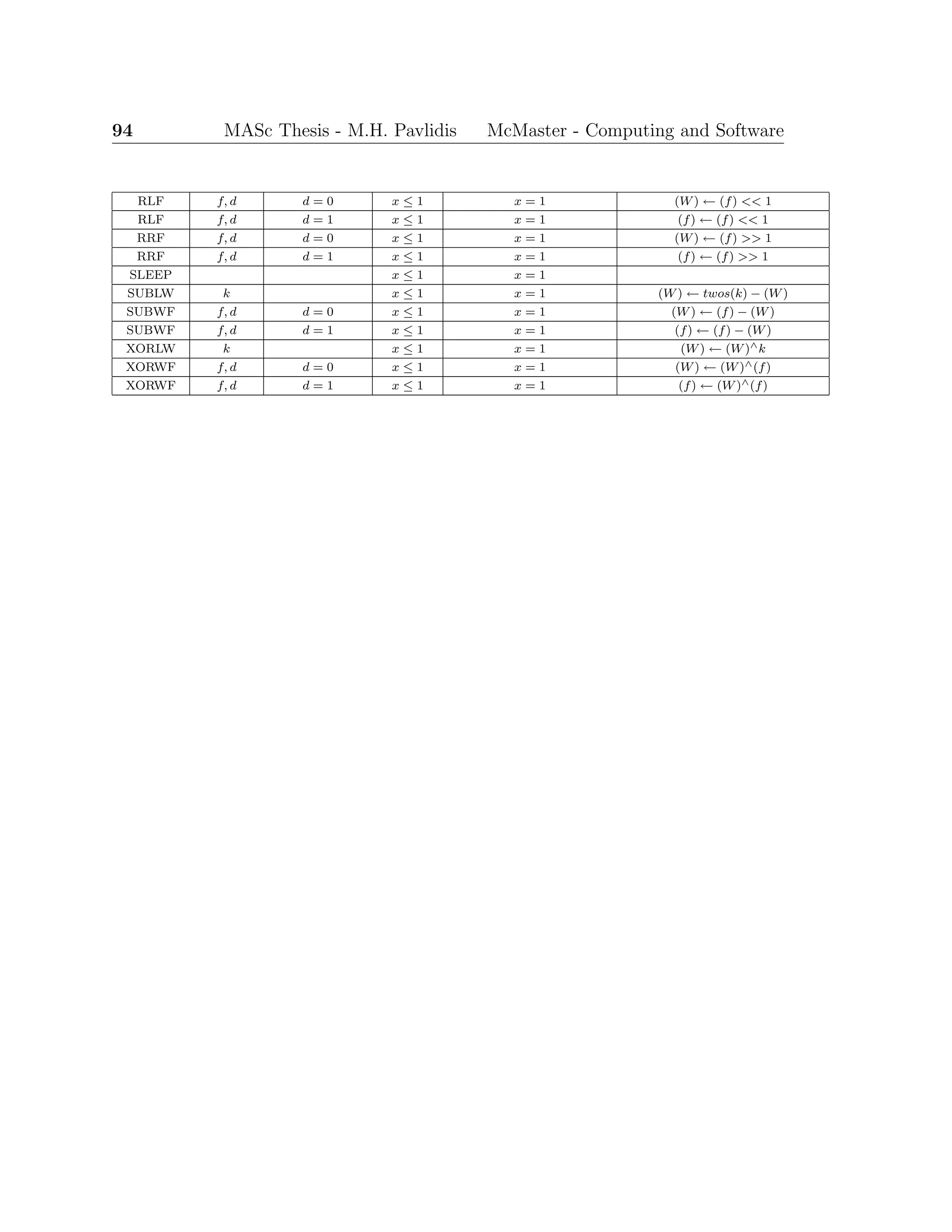
For example, the IBM1800 instruction set’s precise execution time of an instruc-
tion depends on the instruction length of a single- or double-word (i.e., format bit
F = 0 or F = 1, respectively), if the instruction register or index registers are used
(i.e., tag bits T = 0 or T = {1, 2, 3}, respectively), and if indirect addressing is
used. The execution time, or execution cycle count, must be determined for each
case and then converted to the format used in the final stage, namely the timing](https://image.slidesharecdn.com/1cc5036e-53e1-4bf9-87fe-9bea3c729be7-150414001600-conversion-gate01/75/thesis-hyperref-35-2048.jpg)
![MASc Thesis - M.H. Pavlidis McMaster - Computing and Software 23
culating tighter timing results due to the architecture dependent effects of execution
of particular sequences of instructions.
For programs with many branches and/or loops it is obvious that the number
of possible paths quickly explodes. Utilising the fact that path-based methods are
manageable for limited segments of code, such as a single loop or branch path, the
complexity of enumerating the paths is mitigated by decomposing the TG into a
scope graph [12] . A scope graph is constructed from subgraphs of the TG, where each
subgraph is a node representing a scope. Each scope corresponds to a loop or function
contained in the TG subgraph. The WCET calculation then works hierarchically on
the scopes. The longest path must verified to ensure that it is a feasible path. If
it is not, the next longest path is chosen for the WCET calculation and is check for
feasibility. Moreover, for unstructured code (i.e., assembly-level or optimised object
code) it can be difficult to determine the scope that a node of the TG belongs to.
Finally, the task of identifying loops and associated loop bounds must be performed
manually or automatically, prior to the calculation phase of analysis.
Piece-wise calculation strategies, such as the scope graph, result in an overesti-
mated (i.e., less tight) WCET if data-flow information reaches over the borders of
the decomposed pieces. The problem is illustrated by considering a triangular loop,
a nested loop where the number of iterations of the inner loop is dependent on the
iteration count of the outer loop (see Figure 3.1). The inner loop yields a worst-case
iteration bound of 10, as does the outer loop. Thus, the piece-wise calculation over
the path would result in 100 executions of inner loop body, while the actual result
should only be 55.
for(i = 0; i < 10; i++) Outer Loop bound: 10
for(j = i; j < 10; j++) Inner Loop bound: 10
body Piece-wise Execution count: 10 × 10 = 100
Actual Execution count: 10
i=0 i = 55
Figure 3.1: Triganular Loop Example
Path-based calculation methods are useful to obtain explicit execution traces for
timing bounds but are limited by the complexity of the analysed program, yielding](https://image.slidesharecdn.com/1cc5036e-53e1-4bf9-87fe-9bea3c729be7-150414001600-conversion-gate01/75/thesis-hyperref-37-2048.jpg)
![24 MASc Thesis - M.H. Pavlidis McMaster - Computing and Software
safe but less tight results.
3.3.2 Tree-based
Tree-based calculation generates the WCET by a bottom-up traversal of a syntax-
tree of the program. The syntax-tree is a representation of the program where the
nodes describe the structure of the program at the source-code level, and the leaves
represent basic blocks.
The syntax-tree is derived from the flow representation (i.e., timing graph). Tim-
ing is computed by translating each node into an equation that expresses the timing of
its children nodes, then summing the expressions following a set of rules for traversing
the tree.
Tree-based calculation was first introduced by Park and Shaw [32], as timing
schema. It was further extended to include hardware level timing influences, such as
pipelines and cache. It is a simple and efficient method to compute WCET, but it
requires source-level code or highly structured assembly-code. Some instruction sets,
such as the IBM1800 or PIC microcontroller, are inherently unstructured. That is,
branches and loops are not easily identifiable by mechanical or manual methods. Fur-
ther, complier optimisations of object-code results in unstructured code. Therefore,
tree-based calculation is unsuitable for the constraints imposed upon the work of this
thesis, but is feasible in specific cases of small and well-structured source-code.
3.3.3 Implicit Path Enumeration Technique
Due to the space and time complexity issues encountered with the previous calcula-
tion methods, Implicit Path Enumeration Technique (IPET), as the name suggests,
does not find every execution path to determine the WCET. The methods initially
developed in [26, 30, 34] state the problem of finding the WCET by maximising a
sum that is restricted by a set of constraints modeling program flow and hardware
timing (Figure 3.2).
The WCET is found either by constraint solving methods, or more popularly,
by integer linear programming (ILP). The advantages of this method is that each
path does not have be explicitly determined. Instead the behaviour is expressed as
a set of constraints. More importantly, the calculation stage of finding the WCET](https://image.slidesharecdn.com/1cc5036e-53e1-4bf9-87fe-9bea3c729be7-150414001600-conversion-gate01/75/thesis-hyperref-38-2048.jpg)
![MASc Thesis - M.H. Pavlidis McMaster - Computing and Software 25
WCET = max(
i∈BB
xi ∗ ti),
{a set of constrains on ∀i∈BBxi},
where BB is the set of all basic blocks,
xi is the execution count of the basic block,
ti is its execution time.
Figure 3.2: IPET Objective Function and Constraints
is performed by ILP methods and tools (e.g., lp solve() [11]) that are extensively
researched and efficient. This serves to remove the onus on the WCET tools by way of
reuse. An analogous strategy is used for the proposed calculation method described
in the next chapter.
IPET offloads the calculation stage of analysis to other tools, but the earlier
stages of determining loops and loop bounds are still required. Depending on the
analysed code, this process is often done manually and it is tedious and prone to
error. An additional limitation of IPET is that the WCET path is not explicitly
defined. Instead, only a number representing the amount of time or number cycles
the worst-case path would take is reported. Determining the explicit WCET path
requires additional processing. The actual WCET path is valuable information when
analysing the behaviour of the program and requires an additional processing stage to
search for the path. Despite this limitation, IPET is the favoured calculation method
of the popular academic and commercial WCET tools.
3.4 WCET Tools
This section provides an overview of some of the popular timing analysis tools. These
tools are designed to find WCET and they are branded as such, but some are also
capable of determining BCET.
The primary motivation for commercial development of tools is their effective and
efficient use in industry and current practical issues that the theory of static timing
analysis aids in overcoming. Ermedahl has developed the following set of requirements](https://image.slidesharecdn.com/1cc5036e-53e1-4bf9-87fe-9bea3c729be7-150414001600-conversion-gate01/75/thesis-hyperref-39-2048.jpg)
![26 MASc Thesis - M.H. Pavlidis McMaster - Computing and Software
that a WCET tool should support [12]:
• The tool should produce safe and tight estimates of the WCET and provide
deeper insight into the timing behaviour of the analysed program and target
hardware.
• The tool should be reasonably retargetable, supporting several type of proces-
sors with different hardware configurations. It is valuable to provide insight in
how different hardware features will affect the execution time.
• The tool should be able to handle optimised and unstructured code. Also, code
for which some of the source-code is not available (e.g., library functions and
hand-written assembler).
• The tool and analysis should be reasonably automatic, easy to use and should
not require any complex user interaction.
• The user should be able to interact with the tool and provide additional infor-
mation for tightening the WCET estimate, (e.g., constraints on variable values
and information on infeasible paths).
• The user should be able to specify which part of the code to measure, ranging
from individual statements, loops and functions to the whole program.
• The user should be able to view extracted results on both a source code and
object code level. The information should provide insight in code parts which
are executed, and how often.
A survey of available tools, both academic and commercial, yields no tool that
fully supports all of the requirements listed above. The reasons noted for the ab-
sence of such a tool are the complexity in determining precise timing behaviour of
modern processors (with pipelines, caches, branch prediction, etc.), and the fact that
embedded system engineers are unfamiliar with static analysis methods, thus limiting
the market for theses tools. Moreover, there is a belief that the market for timing
analysis tools is small because the number of high-end processors used in embedded
systems is proportionally very small. While this is true for the high-end processors](https://image.slidesharecdn.com/1cc5036e-53e1-4bf9-87fe-9bea3c729be7-150414001600-conversion-gate01/75/thesis-hyperref-40-2048.jpg)
![MASc Thesis - M.H. Pavlidis McMaster - Computing and Software 27
that these tools target, since these tools are primarily focused on solving the hard
problem of processors with high complexity. There is generally a lack of focus on
low-end processors, despite the tremendous market size in terms of volume. The
processor market for 4-, 8-, 16-bit, DSPs and microcontrollers is over 90%, with the
simple 8-bit processors making up 55% of the market. Further, of the less than 10%
market share of 32-bit processors, 98% of those are used in embedded systems [41].
Thus, despite the huge potential market for timing analysis tools for these low-end
processors, the research and industrial communities have largely ignored this market
in favour of attempting to solve more complex problems for processors with a small
market share.
Herein lies the motivation for developing a tool that provides precise timing analy-
sis for high volume, low-end processors. Having the capability of proving that a given
task can safely execute on a less powerful processor yields significant production cost
savings. This is instead of using a much more powerful processor to ensure timing
behaviour is safe but at a higher unit cost.
Another reason for the lack of tools that fully support the list of requirements
is that most tools support WCET analysis at either source-code level or object-code
level. The difficulty these methods introduce is in the mapping of high-level flow
information from source-code down to low-level object-code in order to compute the
timing bounds. The complier is the logical component that links the source-code
flow with the object level timing information. Unfortunately, many compilers are
closed-source provided by the processor manufacturer, and open-source compliers
(i.e., gcc[16]) generate much less efficient object code.
Obtaining the flow of data information (e.g., loop bounds) automatically from
source code is significantly less complex than from object code, that requires main-
taining flow of data between registers and memory. For the Reverse Engineering
project, we are in effect only considering the latter case because the program was
implemented in assembly. Further, at the source level the variable names are more
meaningful to the analyst than memory and register addresses. Regardless of whether
the methods to obtain loop bounds operate on source- or object-code are manual or
automatic, the problem of converting the information into a form for the calculation
state remains.
Academic WCET tools have developed out of the motivation for a proof-of-concept](https://image.slidesharecdn.com/1cc5036e-53e1-4bf9-87fe-9bea3c729be7-150414001600-conversion-gate01/75/thesis-hyperref-41-2048.jpg)
![28 MASc Thesis - M.H. Pavlidis McMaster - Computing and Software
implementation of a new theoretical approach, or to provide a set of functions that
allow for theory to be examined and extended. Development of the academic type of
tools tends to stall once it reaches a desired level of stability, or the researchers move
on to other areas of interest.
One such example is the research prototype Cinderella [25], developed at Princeton
University, that has not been actively developed for ten years. Cinderella determines
both BCET and WCET for the Intel i910 and Motorola M68000 processors. It pro-
vides a graphical development environment from source-code to object-code, and the
mapping between them.
In Cinderella, timing bound calculation is based on the IPET developed by Li
and Malik [26]. The tool determines the linear constraints for cache and pipeline
behaviour of the processors, but requires manual annotation of flow behaviour to
tighten the timing bounds. For example, the triangular loop problem (Figure 3.1)
would require the analyst to determine the linear constraint x3 = 55 x1, where x1
represents the outer for-loop’s basic block, and x3 represents the inner-loop body’s
basic block. Another limitation of the prototype is that it does not provide the
best- and worst-case execution paths because it depends on IPET for timing bound
calculation.
The tool provides the capability to retarget the timing bound estimation of differ-
ent hardware platforms through a well-defined C++ interface. Retargeting requires
the implementation of backends for the object file, instruction set, and machine model.
Cinderella provides a good model of modularisation to separate the computation and
interface implementation from the backend modules that perform the control flow
and low-level analysis.
Other academic tools are prototype research implementations strictly focused on
source-code level dependent analysis. These are not feasible to extend for this work
due to the dependence on high-level source-code and manual annotation requirements.
They include Calc wcet 167 [40] that is an implementation of Kirner and Puschner
[21] for the Siemens C167CR processor from the Vienna University of Technology
and Heptane [2] static WCET analyzer for several processors from ACES Group at
IRISA.
Some research projects have evolved into commercial products. One such tool
is Bound-T [39] from Tidorum Ltd. in Finland. Bound-T supports several architec-](https://image.slidesharecdn.com/1cc5036e-53e1-4bf9-87fe-9bea3c729be7-150414001600-conversion-gate01/75/thesis-hyperref-42-2048.jpg)
![MASc Thesis - M.H. Pavlidis McMaster - Computing and Software 29
tures and analyses machine-level code to compute WCET and its execution path.
It automatically determines loop bounds for counter-type loops and allows for user
assertions on the program behaviour. Another commercial tool is aiT [1], an im-
plementation of the Abstract Interpretation and ILP method developed by Theiling
et al[38]. aiT is targeted for high-end processors with cache and pipelines and it
computes the WCET and graphically displays the worse-case execution path, but
aiT requires manual annotations of loop and recursion bounds and does not find the
BCET.](https://image.slidesharecdn.com/1cc5036e-53e1-4bf9-87fe-9bea3c729be7-150414001600-conversion-gate01/75/thesis-hyperref-43-2048.jpg)

![32 MASc Thesis - M.H. Pavlidis McMaster - Computing and Software
4.1.1 Timed Automata
The original theory of timed automata was developed by Alur and Dill [5, 6], for
modeling and verifying real-time systems. A continuous-time timed automaton model
is a finite-state B¨uchi automaton with a finite set of non-negative real-valued clocks.
The automaton is an abstract model of a real-time system, providing a state transition
system of the modeled system. It is represented as a directed graph, with nodes
representing locations and edges representing transitions.
Constraints on the clocks are used to restrict the behaviour of the automaton
and enforce progress properties. Clock constraints on locations, called invariant con-
ditions, are invariants forcing a transition when the state would violate the clock
invariant.
Transitions of the automaton have clock constraints guarding the transition edge,
called triggering conditions, restricting when a transition can be enabled based on the
clock guard. Transitions include clock resets, where some clock variables are reset to
zero.
Describing a complete system in one timed automaton is large and cumbersome,
thus TA have been extended with communication signals on transitions. The real-
time system can then be described as a set of timed automata, with each process of
the system decomposed into its own automata. Later, the theory of timed automata
was later extended by Bengtsson et al. [8], to include data variables in the state space,
that can be used in transition guards and updates.
4.1.2 Model Checking
Given a real-time system modeled as a timed automaton, system properties can be
expressed as temporal logic formulas and model checked. The temporal logic com-
monly used is Timed Computation Tree Logic (TCTL) [4], and is used to express
safety and liveness properties of the system. Model checkers search the automata
state space exhaustively until a counterexample is found to refute a claimed system
property of the model. Due to the potential of state space explosion, model checker
implementations use data structures, approximation methods, and symbolic states to
efficiently represent and search the state space. Further, some model checkers (e.g.,
Uppaal) restrict clock guards to maintain convex zones and check only a subset of](https://image.slidesharecdn.com/1cc5036e-53e1-4bf9-87fe-9bea3c729be7-150414001600-conversion-gate01/75/thesis-hyperref-46-2048.jpg)
![MASc Thesis - M.H. Pavlidis McMaster - Computing and Software 33
TCTL formulae. Consequently, the model checking results are generated faster, in
less space, making checking of larger models feasible.
Model checking has proven to be very successful in the verification of system
requirements and design models against system specification properties. In particular,
model checking has been used in practice for verifying real-time embedded safety-
critical systems design, potentially identifying design errors early in the development
cycle. The behaviour of the system design is modeled according to the state transition
system notation used by the model checker (e.g., timed automata) with respect to
high-level abstract actions that the system performs. The model is created manually
by, or in collaboration with, a domain expert of the system, and care must be taken
to accurately represent the system.
The model representation of the system abstracts away the details of the under-
lying software and hardware systems execution, and only models significant timing
events [15] (e.g., deadlines, periods, feasible WCET). When the design model success-
fully verifies against the specification properties, the system is implemented accord-
ing to the design in the selected programming language and compiled for the target
hardware. Foreshadowing our method proposed in the next section, an interesting
observation can be made; although model checking is a widely accepted method of
verifying the system design, attempts to verify system implementations are typically
done by executing test cases on the implementation and/or manual inspection.
4.1.3 Model Checking Implementations
Published examples of the use of model checking representations of implementations
are sparse. One such example, by Fidge and Cook [15], is a case study that investi-
gated the behaviour of interrupt-driven software.
The case study models the assembly code of an aircraft altitude computation
and display program, to be referred to as Altitude Display, that reads an altimeter
and computes an estimate for the aircraft’s altitude. The program asynchronously
requests the current value from the altimeter and the value is returned to the program
by way of an interrupt. While waiting for the interrupt, the program computes an
estimate of the altitude. If the interrupt from the altimeter does not arrive in time,
the estimate is displayed instead of the actual value returned from the altimeter. The](https://image.slidesharecdn.com/1cc5036e-53e1-4bf9-87fe-9bea3c729be7-150414001600-conversion-gate01/75/thesis-hyperref-47-2048.jpg)
![34 MASc Thesis - M.H. Pavlidis McMaster - Computing and Software
assembly code is modeled in the Symbolic Analysis Laboratory (SAL, one of the SRI
FormalWare tools)[35], with each state representing a basic block of assembly code.
The motivation for the case study is an interest in the behaviour of the interrupt-
driven program, that depends on the relative arrivals of the interrupt over time and
its impact on the accuracy of the altitude displayed. Instead of modeling all possible
interrupt points, only those points in time when significant events occur (i.e., the
cases when the altimeter responds on time or not) are modelled. Many equivalent
states are thereby eliminated when modelling interrupt behaviour of the program’s
execution.
Model checkers, such as SAL, exhaustively search the state space until a coun-
terexample is found to refute a claimed property of the model, or the system is found
to satisfy the property. In the case of SAL’s Bounded Model Checker and the model
of the Altitude Display program, the property claim is a temporal logic formula as-
serting reachability of the last instruction. Modeling the Altitude Display task in SAL
involves understanding the behaviour of the code and manually modeling its effects
on the register and memory values, program flow (i.e., assignment of the program
counter), and the instruction cycle execution time of each action. The first is directly
translated from the assembly code, while the latter two are implicitly described in
the code and require knowledge of the hardware environment for precise execution
time and program counter assignment. The execution time is modeled by a variable,
Now, of type Time, that is used to guard actions and is updated on the transitions
with a value representing the execution time of the instructions model by the associ-
ated action. Moreover, the interrupt behaviour of the hardware is used to model the
different possible significant events, modeling equivalent actions. Thus, a limitation
of the method is that it requires complete understanding of the given assembly code
and hardware environment to correctly manually model the task.
A further limitation of the method presented by Fidge [15] that prevents it from
being used to obtain timing bounds from model checking is that SAL searches for
the shortest counterexample to the property given as a temporal logic formula. In
this case, it would be a reachability property to the guarded action representing
the last basic block of assembly code. The counterexample found is the shortest
trace, in terms of number of transitions, through the model representing the program
code. Thus, SAL’s Bounded Model Checker is not capable of finding the fastest and](https://image.slidesharecdn.com/1cc5036e-53e1-4bf9-87fe-9bea3c729be7-150414001600-conversion-gate01/75/thesis-hyperref-48-2048.jpg)
![MASc Thesis - M.H. Pavlidis McMaster - Computing and Software 35
slowest traces, with respect to the variable modeling time, because its search does
not explicitly take time (or time variables) into consideration when searching for the
counterexample. Moreover, there is no way to express the temporal logic property
to find fastest/slowest timed traces. Therefore, in its current form, the SAL model
checker is not a feasible tool to use to find timing bounds of program implementations
by model checking.
4.1.4 Timing Analysis by Model Checking
The lack of publications in the area of performing timing analysis with model check-
ing possibly indicates that model checking alternatives do not offer advantages to the
present static timing analysis methods. Wilhelm [46] presents several methods for
using model checking and argues that none offer acceptable performance. The solu-
tions focused on target hardware with cache, which this thesis does not address, but
the method applies this work. The cited problems with the model checking methods
were that the state space is too large or require too many model checking iterations
to find a precise upper bound.
Metzner [28] countered the argument that model checking is adequate for finding
timing bounds and, furthermore, can improve the results. The method models the
program and its interaction with the hardware as an automaton. The automaton
includes a set of variables, some of which are used to track time consumed. It begins
with the source C program with annotation to bound loop iterations. The annotations
are preserved in the translation into assembly code. The assembly code is used to
generate an automaton. The automaton representation is a C program that is used
as input to the OFFIS verification environment. The automaton is model checked
for a reachability query to a termination point for some cycles bound N. Based on
the result, the bound is then increased or decreased as appropriate until a tight value
is obtained for the upper bound of execution cycles. Typically the approach uses a
binary search method to choose the next attempt for N. The experimental results
revealed that the multiple model checking iterations do not lead to an infeasible
method.
Metzner’s method and results indicate that timing analysis by model checking
is feasible. It finds a precise bound and provides a concrete execution path for the](https://image.slidesharecdn.com/1cc5036e-53e1-4bf9-87fe-9bea3c729be7-150414001600-conversion-gate01/75/thesis-hyperref-49-2048.jpg)
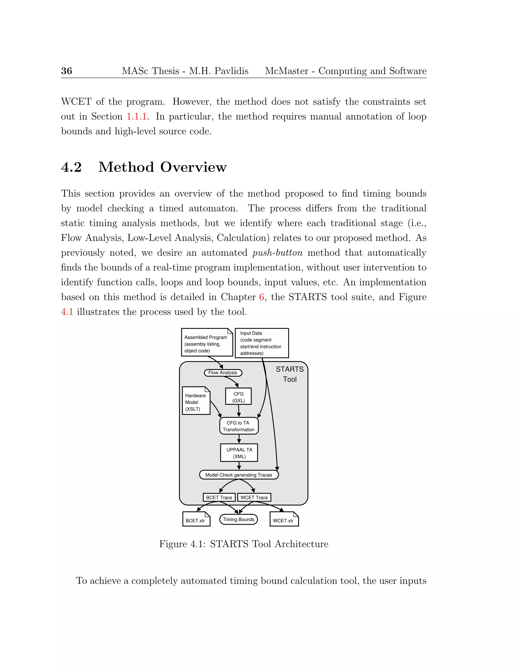
![MASc Thesis - M.H. Pavlidis McMaster - Computing and Software 41
4.2.4 Calculating Timing Bounds
Creating a TA model from the CFG, followed by annotating the model with timing
information from the Hardware Model and data flow information from the CFG an-
notation, results in a precise model of the program execution. Further, the model
includes clock invariants, guards, and updates that provide the precise clock delay of
the actual program execution.
The model checker must feature the capability to find the fastest and slowest traces
based on the accumulated clock delay of the TA model (e.g., as is done in a prototype
version of Uppaal). The real-time model checker can be used to calculate the timing
of the BCET and WCET of the program. The reachability checker for the slowest
trace must include the capability to detect infinite loops and ensure termination, as
Uppaal provides [7].
The model checker attempts to verify a reachability property from the initial
location (i.e., the user given start instruction address) to the end location (i.e., the
given end instruction address). Instructing the model checker to generate fastest
and slowest witnessing traces when verifying the reachability property produces the
BCET and WCET traces, respectively, for the modeled program. The value of the
accumulated clock delay at the end of the trace represents the number of clock cycles
the trace execution would require on the target microprocessor. If the clock rate of
the target processor is known, the program’s timing bounds could also be expressed
in units of time.](https://image.slidesharecdn.com/1cc5036e-53e1-4bf9-87fe-9bea3c729be7-150414001600-conversion-gate01/75/thesis-hyperref-55-2048.jpg)

![Chapter 5
A Timing Analysis Transformation
System
The details of the transformation process from machine-code representation to CFG,
and CFG to TA, previously described are presented in this chapter. The primary focus
is on the latter transformation of the CFG representation of the program instructions
to a TA model that describes the execution of the instructions. The instruction
set operations are decomposed into six types of transformations, categorised by the
instruction’s effects on control- and data-flow. The TA model obtained from the
transformations is used to determine the BCET and WCET of the program.
5.1 Control Flow Graph Representation
The transformation from assembly- or machine-code to a static CFG representation
is the first step of the process to generate a TA that can be used for timing analysis.
The primary contribution of this thesis is the timing analysis of real-time programs by
model checking Timed Automata. Thus, the details of the CFG generation is outside
its scope. The reader is referred to [37, 23, 21, 45] for in-depth details of how the
graph representing execution paths of the program is constructed. Here, we limit the
description of the CFG to what is required to proceed to the next processing step,
transformation to a TA.
With respect to the transformation process, it is assumed that all the paths
43](https://image.slidesharecdn.com/1cc5036e-53e1-4bf9-87fe-9bea3c729be7-150414001600-conversion-gate01/75/thesis-hyperref-57-2048.jpg)
![44 MASc Thesis - M.H. Pavlidis McMaster - Computing and Software
through the CFG represent at least all the feasible execution paths of the program.
The transformation to a TA requires the CFG nodes to be annotated with specific
relevant instruction information (i.e., instruction address, opcode, operands, etc.).
A complete list of the required information depends on the instruction set and the
hardware architecture. Thus, the precise node annotations will vary between target
architectures. In general, the annotations must include all the fields of the assembly
code instruction and the instruction address. The information in the annotated CFG
is combined with the Hardware Model of the target architecture to transform the
model into a TA describing the behaviour of the program’s execution.
5.2 Timed Automata Representation
The second step of the transformation process is from the CFG representation of the
program to a TA model. The model is transformed into a format that can be used
with TA model checker that will generate the BCET and WCET.
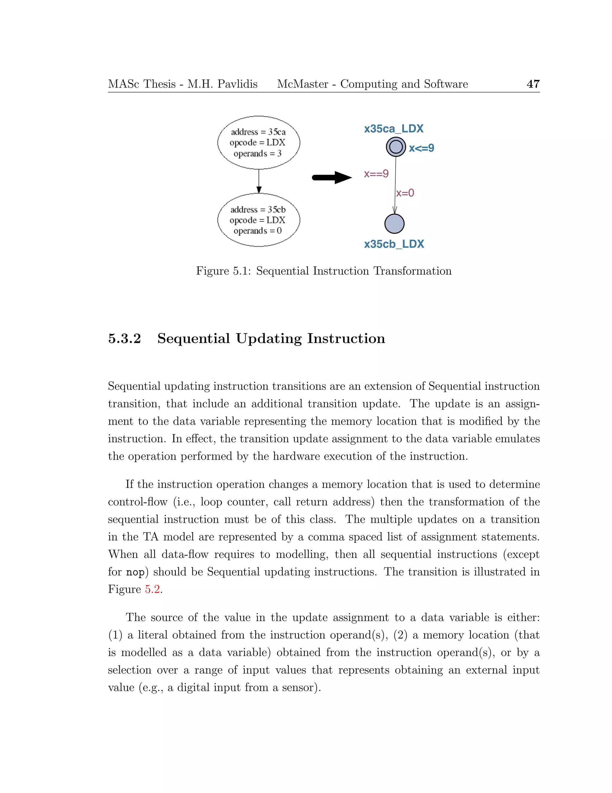
The instructions of the program, represented as the nodes of the CFG, are mapped
directly to locations in the TA. The execution time of each instruction is represented
by a clock invariant on the location of the form x ≤ n, where x is a clock maintaining
the instruction execution time, and n ∈ N. The units of n may be a clock cycle,
an instruction cycle, or the smallest fraction of instruction execution time, and is
defined in the Hardware Model. The invariant creates a delay transition in the TA
that represents the passage of time (clock cycles) for the execution of the instruction,
by allowing the TA to remain at the location. The invariant forces one of the feasible
action transitions to occur when the delay at the location equals the execution time.
The action transitions include a clock guard, of the form x == n, that prevents the
transition from occurring early.
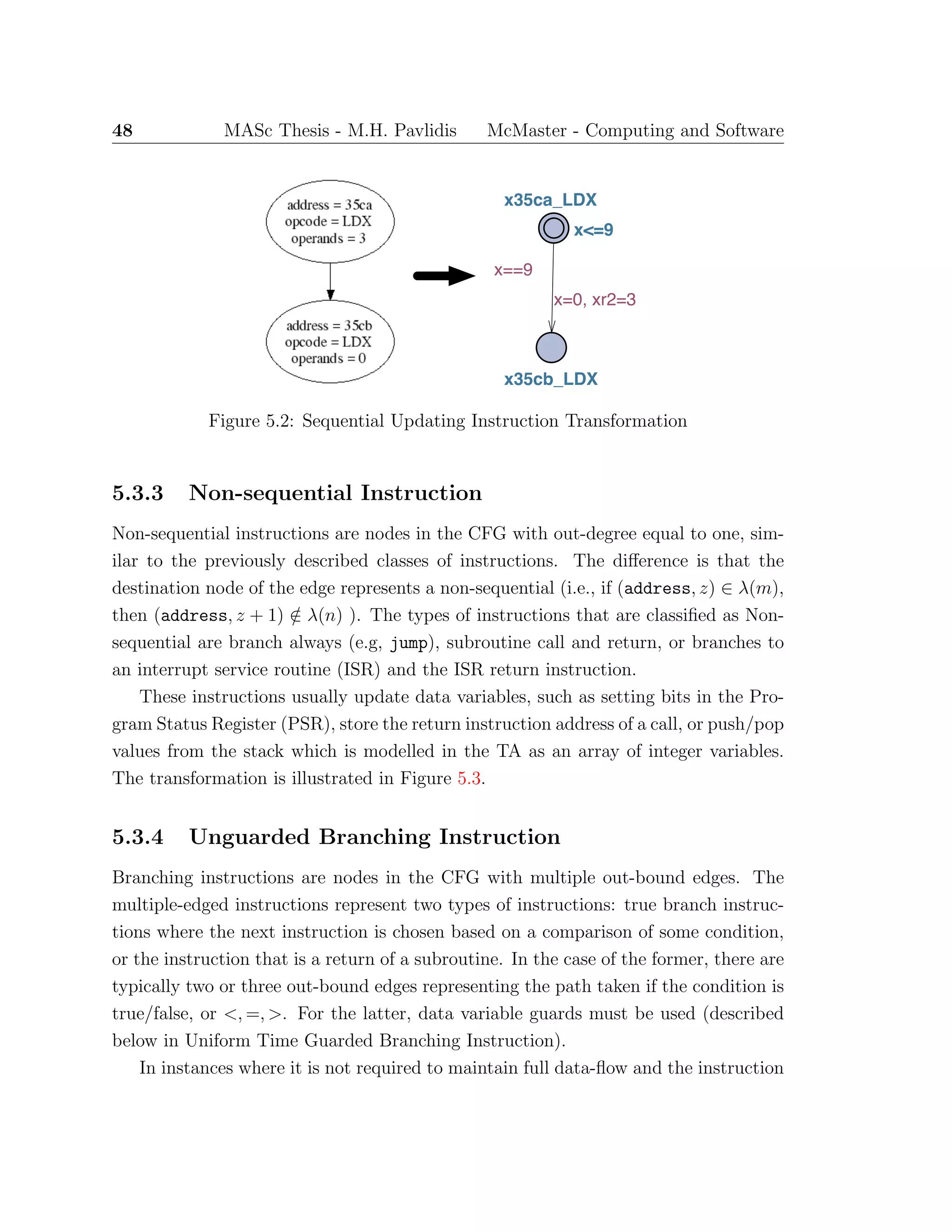
The action transitions indicate the possible subsequent executable instructions.
Each transition includes the clock guard described above, that enforces the instruc-
tion’s execution time, and a reset of the clock (i.e., v[x := 0]) for the next location.
Additional data variable guards are added to restrict the possible traces to feasible
execution traces. For example, if memory location x34B1 stores a loop bound, and
x34B0 stores a loop counter, then the transition that represents exiting a loop will
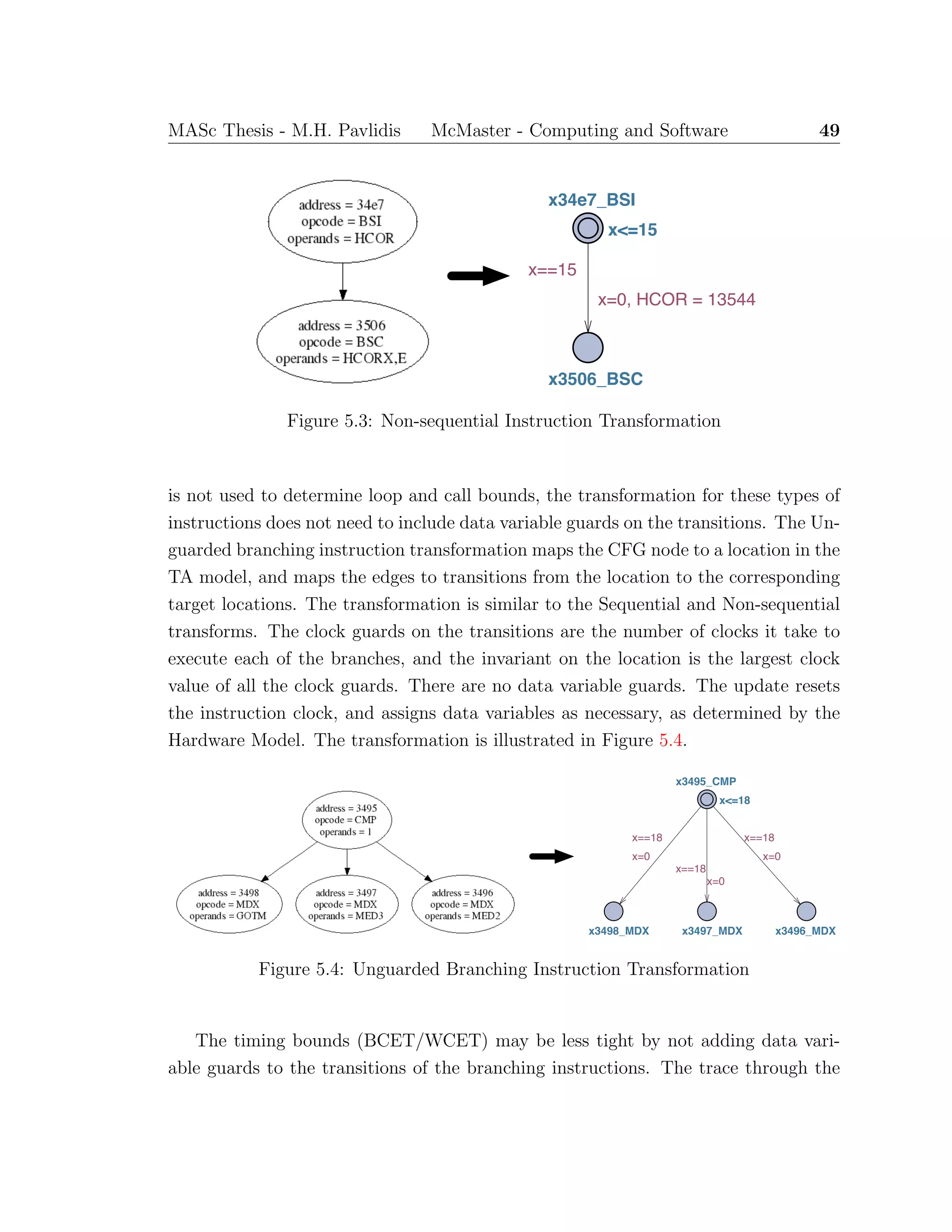
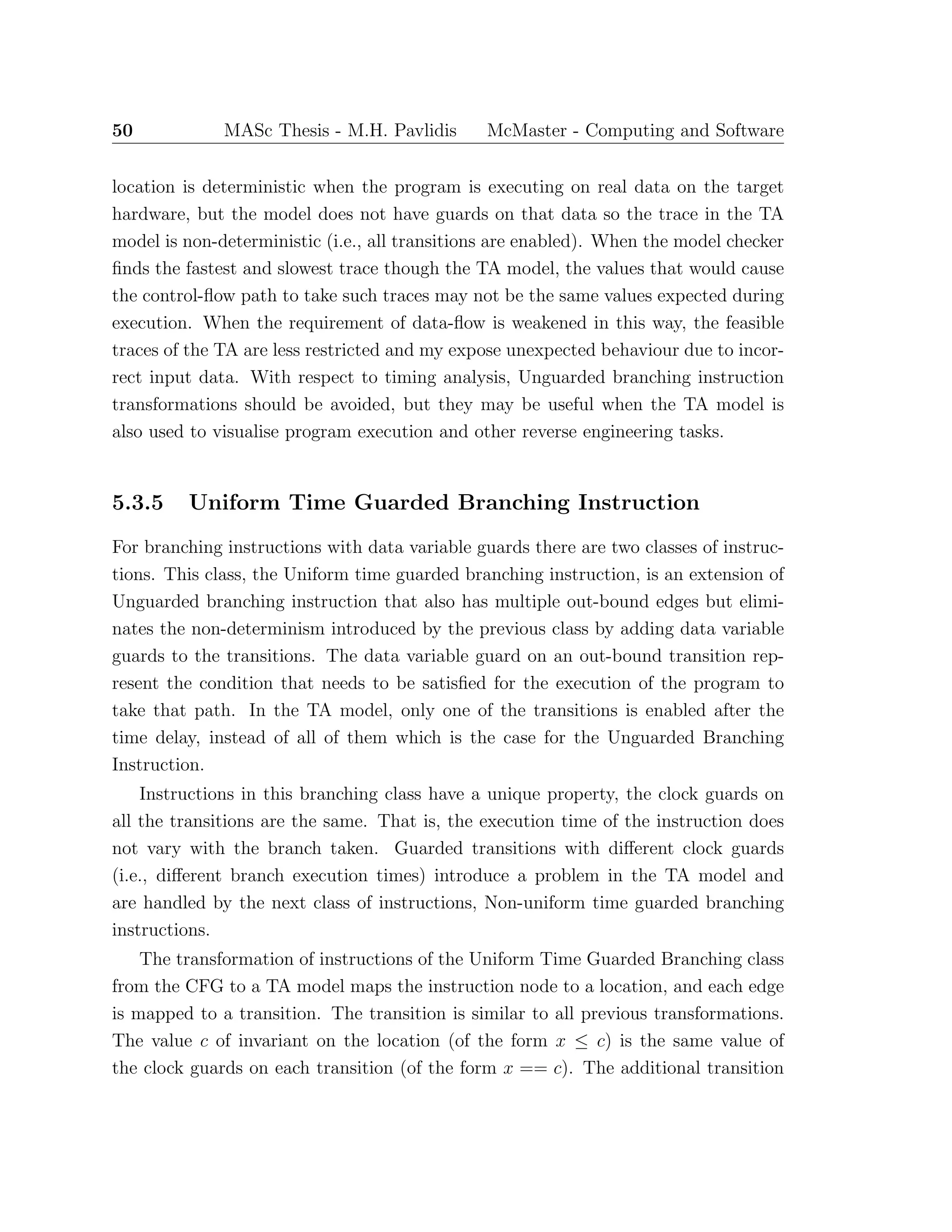
have a variable guard of the form, x34B0 ≥ x34B1. Similarly, a transition from some](https://image.slidesharecdn.com/1cc5036e-53e1-4bf9-87fe-9bea3c729be7-150414001600-conversion-gate01/75/thesis-hyperref-58-2048.jpg)
![52 MASc Thesis - M.H. Pavlidis McMaster - Computing and Software
ss
x10d_retlw
x<=2
x8e_swapf
xba_swapf
xda_btfss
x==2
&& stack[tos-1] == 142
x=0, tos--
x==2
&& stack[tos-1] == 186
x=0, tos--
x==2
&& stack[tos-1] == 218
x=0, tos--
Figure 5.6: Return Instruction Transformation
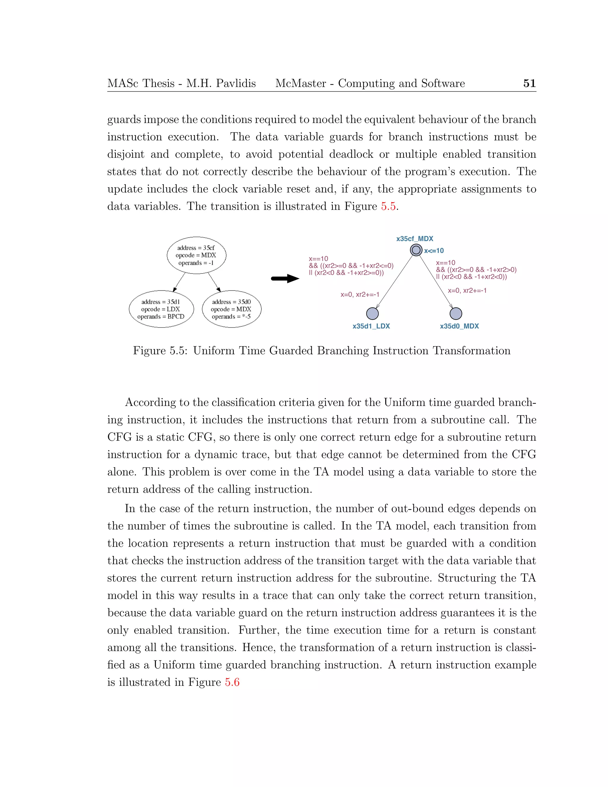
5.3.6 Non-Uniform Time Guarded Branching Instruction
Non-uniform time guarded branching instructions are similar to instructions of the
previous class, but differ in one important aspect. The execution time of the multiple
transitions take different clock times. If the clock guards are transformed using the
method applied for Uniform Time Guarded Branching instruction of the previous
subsection, deadlock states are introduced into the TA model when no deadlock occurs
in the program.
The potential deadlock in the model stems from the fact that the invariant on the
location must be the largest clock value of all the transition clock guard values. The
invariant allows for a delay transition to model the execution time of the instruction.
As a result, the invariant value must be the maximum clock delay. The data variable
guards on the transitions of a branching instruction are disjoint and complete. Based
on the value of the data variable in the guard, only one of the multiple transitions
is enabled, and that occurs only when the instruction clock satisfies the clock guard.
An example of the TA model is illustrated in Figure 5.7.
The deadlock state is introduced when the transition has a satisfied data variable
guard and a clock guard with a value less than the maximum embodied by invariant
value. The transition is only enabled when the clock guard is satisfied. That is, at the
value of the clock variable that represents the execution time of taking that branch.
In this case, TA model does not force taking the enabled transition, because it can
remain at the location while the clock invariant is satisfied. In this case, there are no
enabled transitions when the instruction clock reaches its upper bound enforced by](https://image.slidesharecdn.com/1cc5036e-53e1-4bf9-87fe-9bea3c729be7-150414001600-conversion-gate01/75/thesis-hyperref-66-2048.jpg)
![MASc Thesis - M.H. Pavlidis McMaster - Computing and Software 53
xda_btfss
x<=2
xdb_goto xdc_bsf
x==1
&& (dr[128*b+41] & pow(2,7))==0
x=0
x==2
&& (dr[128*b+41] & pow(2,7))!=0
x=0
Figure 5.7: Potential Deadlock on Guarded Branching Instruction Transformation
the invariant. Therefore, the model checker identifies a deadlock state that does not
accurately reflect the behaviour of the program.
To overcome the introduction of a deadlock state that does not occur in the
program code, the mapping of location and edges does not follow the typical one-to-
one as with all other transformations. The instructions of this transform class have a
one-to-(n + 1) node to location mapping, where n is the number of out-bound edges.
Similar to the previous transforms, one of the locations represents the instruction.
This location is an urgent location (i.e., time is not allowed to pass in an urgent
location), so it does not model the execution time delay of the instruction. It is the
target of all in-bound transitions to the instruction and has n data variable guarded
transitions representing the paths to the subsequent instructions. The targets of these
transitions are not the next instruction locations, rather they are auxiliary locations
create by the transformation. The auxiliary locations model the execution time of the
instruction, thus the transformation puts the clock invariant on the auxiliary location
for each branch.
The edges of the CFG that represent the possible branches of the instruction are
mapped one-to-two into transitions in the TA model. The first transition is from the
instruction location to the respective auxiliary location. There is no update assign-
ment or clock guard on the transition. The only guard is the data variable guard
representing the condition that needs to be satisfied to take the branch. The second
transition is from the auxiliary location to the instruction location that represents the
target of the edge from the CFG. This transition is annotated with all the the appro-](https://image.slidesharecdn.com/1cc5036e-53e1-4bf9-87fe-9bea3c729be7-150414001600-conversion-gate01/75/thesis-hyperref-67-2048.jpg)
![54 MASc Thesis - M.H. Pavlidis McMaster - Computing and Software
priate guards and updates (similar to the previous classes of transformations). The
transition guard includes the clock guard that models execution time, and the same
data variable guard from the first mapped transition. It also includes a reset of the
instruction clock, and any necessary data variable assignments. This transformation
is illustrated in Figure 5.8.
ss
xda_btfss
x<=1 x<=2
xdb_goto xdc_bsf
(dr[128*b+41] & pow(2,7)) == 0
x==1
&& (dr[128*b+41] & pow(2,7))==0
x=0
(dr[128*b+41] & pow(2,7))!=0
x==2
&& (dr[128*b+41] & pow(2,7))!=0
x=0
Figure 5.8: Non-Uniform Time Guarded Branching Instruction Transformation
5.4 Summary
The TA model generated by the transformations on the CFG describes the timing
and behaviour of the source assembly program. The execution time of the instruction
is modelled by the delay transition that is caused by the combination of the clock
invariant on the location and the clock guard on transitions. The behaviour of the
the program is modelled by the data variable guards and data variable update on the
transitions. The updates emulate the program’s assignments to memory locations,
and the guards restrict the traces through the model to only the feasible execution
traces.
With a formalisation of the transformations, the behaviour of the program de-
scribed by the TA model can be proven correct (i.e., the model includes only the
feasible traces) using structural induction over the instructions of the program. In-
formally, it is shown that the behaviour described by the TA model is correct because
the result of the transformation of each instruction exhibits the same operations that
occur in the processor executing the machine code.](https://image.slidesharecdn.com/1cc5036e-53e1-4bf9-87fe-9bea3c729be7-150414001600-conversion-gate01/75/thesis-hyperref-68-2048.jpg)

![68 MASc Thesis - M.H. Pavlidis McMaster - Computing and Software
CFG is generated that includes only the connected instruction nodes of the function.
The BPC functions analysed include Boiler Pressure Median (MEDIAN), Corrected
Hilborn Average (HLBN), Setback Majority Vote (DI2F3), and the Turbine Feedback
Calculation (TRBFB) that also calls DI2F3 . The TRBFBns is the same function but the
path that shortcuts the feedback calculation is made unfeasible. The last example
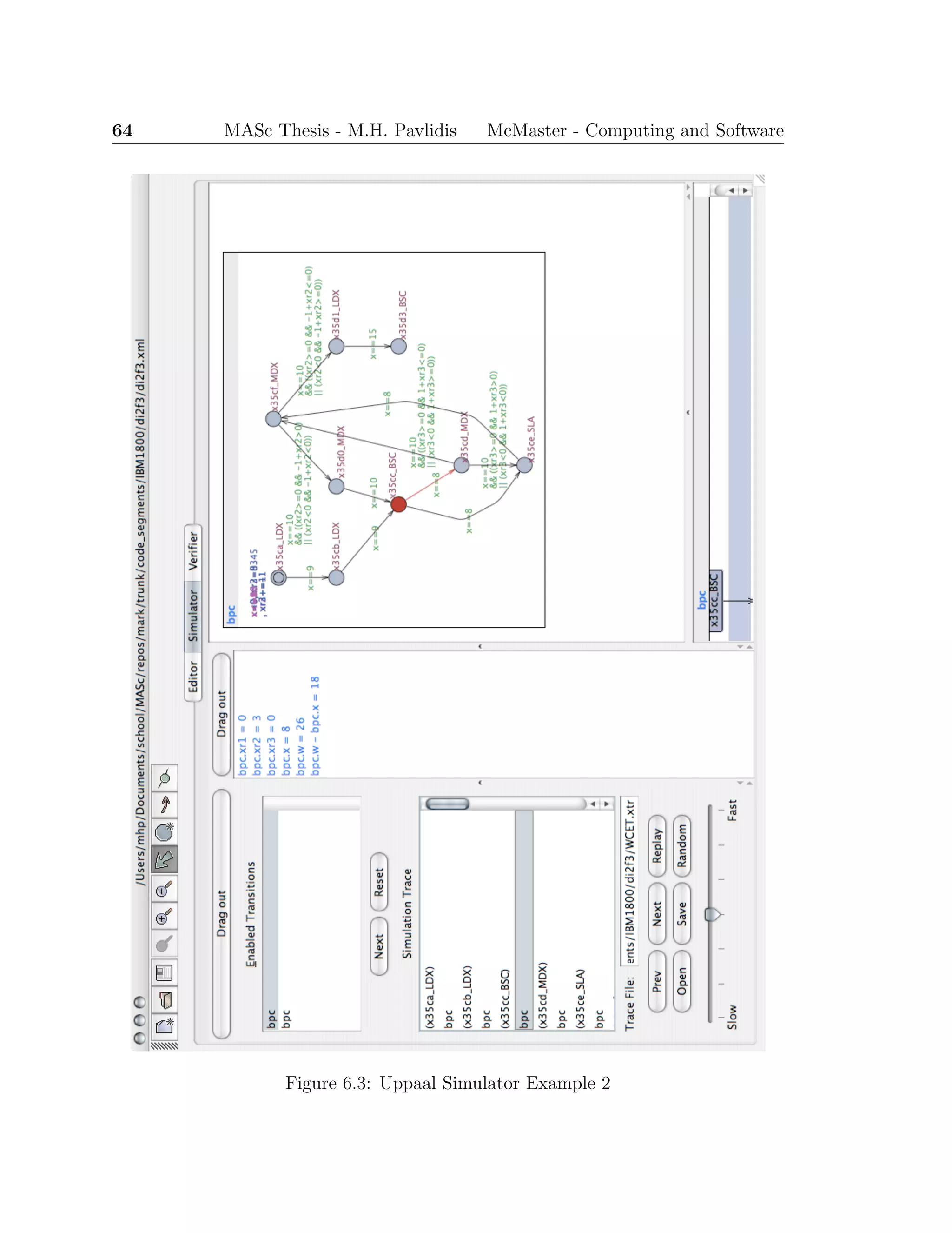
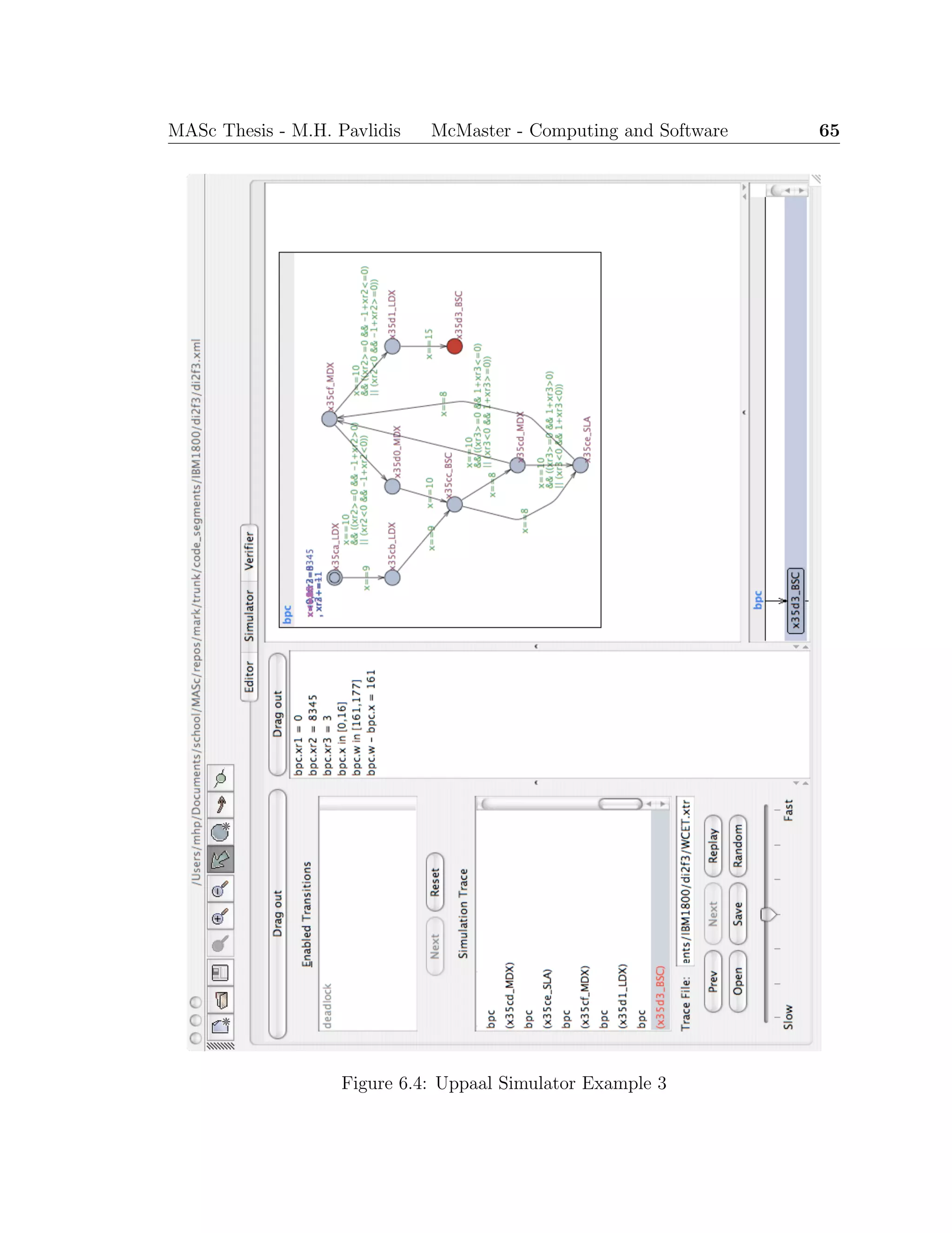
demonstrates the different traces through the DI2F3 subroutine that affects the branch
taken after the subroutine has completed for the BCET and WCET traces of the
feedback calculation.
The code examples were small enough to allow manual verification of the results
generated by the STARTS tool suite is correct and presented in Table 7.1.
Table 7.1: IBM1800 BPC Results
Function BCET (clocks) BCET (µs) WCET (clocks) WCET (µs)
MEDIAN 45 10.25 143 35.75
HLBN 1437 359.25 4461 1115.25
DI2F3 147 36.75 177 44.25
TRBFB 452 113 771 192.75
TRBFBns 646 161.5 771 192.75
Sun [36] analysed the same TRBFB segment of code with the WCET tool he im-
plemented. The worse-case execution path generated by the tool is exactly the same
at the WCET trace generated by Uppaal. Sun’s WCET reported by the tool was
189.5 ms (units should be µs). The difference from the STARTS output of 192.75 µs
is attributed to small differences in the execution time assigned to some instructions.
For example, the first LD instruction of the code segment is 3.75 µs in Sun’s work, but
17 clocks (or 4.25 µs) in the STARTS hardware model. The execution time of each
instruction was obtained from the IBM1800 Functional Characteristics manual [20].
The source of the discrepancy in instruction execution times could not be determined.
7.3 PIC Timing Analysis Results
The program used to experiment with the PIC implementation of the STARTS tool
suite was a Software PID Control of an Inverted Pendulum Using the PIC16F684](https://image.slidesharecdn.com/1cc5036e-53e1-4bf9-87fe-9bea3c729be7-150414001600-conversion-gate01/75/thesis-hyperref-82-2048.jpg)
![MASc Thesis - M.H. Pavlidis McMaster - Computing and Software 69
[9] provided by Microchip. The assembly code implementation includes loops, sub-
routine calls, A/D input conversion, and an ISR. Experimentation with the code
provided insights in to handling data-flow, subroutine calls, and additional hardware
functionality.
The assembly code of the inverted pendulum controller was modified by a student
for a graduate course project. The project was to design and implement a controller
that stabilises the magnetic levitation of a permanent magnet beneath a solenoid by
controlling the current flow and direction through the solenoid. The program is a
busy-wait loop that modifies the output of the program’s feedback control loop after
the ISR updates the input sensor value. The ISR is triggered by an internal clock
timer initially set to update the input value, and accordingly execute the feedback
control loop to modify the output value, every 256Hz. The implementation of the
magnetic levitation controller realised a system that would not remain stable for
longer than short periods of time.
Analysing the implementation with the STARTS tool, the WCET of the feedback
control loop was calculated to be 867 cycles, and the WCET of the ISR was 51 cycles.
Thus the combined worse-case execution time of the ISR and the feedback control loop
was 918 cycles, or 114.75µs. The combined execution time is the minimum period
required for the interrupt timer. By identifying the WCET of the feedback control
loop and the ISR, the maximum frequency of the interrupt timer was computed to
be 8714Hz. Therefore the setting for the clock timer to interrupt was changed from
256Hz to 8kHz, and increasing the response rate resulted in a stable system.](https://image.slidesharecdn.com/1cc5036e-53e1-4bf9-87fe-9bea3c729be7-150414001600-conversion-gate01/75/thesis-hyperref-83-2048.jpg)

![74 MASc Thesis - M.H. Pavlidis McMaster - Computing and Software
instruction in the program where the deadlock or livelock occurs. When generating
the WCET trace, this property is checked prior to generating the trace to ensure
termination of the worse-case trace.
Reachability properties (i.e, E<> p) to instructions of interest can be used to verify
that instructions of the implementation are on a feasible execution path. That is, the
instruction is reachable from the beginning of the program (i.e., helping to identify
dead code). With traces enabled, if the property is satisfied then a trace will be
generated to the instruction that can be used for further analysis of the program’s
functional and timing behaviour.
Safety properties of the program can be verified with the above temporal prop-
erties to ensure an instruction is reached, or that it is reached within a specific time
limit. Another safety property that can be verified makes use of the leads to (i.e.,
p --> q) property, meaning whenever p holds eventually q will hold as well. p --> q
is equivalent to A[] (p imply A<> q). This property can be used to verify that an
instruction will always be executed at some point after some other instruction. An
example is a safety property that states: if a shutdown signal is detected the sys-
tem must shutdown. Whether the implementation satisfies the safety property can
be verified by checking the property p --> q, where p is the instruction where the
shutdown signal is detected and q is the instruction that shutdowns the system.
Other properties can be verified with respect to execution states of the program,
values or range of values on inputs or memory locations. Thus, the TA model of
program can be used for numerous tasks other than finding timing bounds. It is useful
in forward development to verify system requirements, and for the identification of
system requirements in reverse development.
8.1.5 Execution Path Visualisation
In addition to verifying specific properties of a real-time program, the model can be
used to effectively emulate the program’s execution. Using the Simulator component
of Uppaal, the execution path of the program is visualised graphically. Input values
and locations with multiple enabled transitions can be selected manually and the
resulting traces examined.
The visualisation can be used in reverse engineering efforts to facilitate under-](https://image.slidesharecdn.com/1cc5036e-53e1-4bf9-87fe-9bea3c729be7-150414001600-conversion-gate01/75/thesis-hyperref-88-2048.jpg)
![MASc Thesis - M.H. Pavlidis McMaster - Computing and Software 77
some other memory location variable. Such a method could possibly use a function1
to set or return the appropriate value.
The current control-flow graph generation tools do not maintain information re-
quired to include branching to instructions via indirect addressing. The indirect
branching must be included in the CFG for the indirect branching transitions to be
included in the model. Further, the model must support indirect addressing if the
transitions of an indirect branch are guarded with the target instruction address (e.g.,
indirect reference to a return instruction address).
8.2.2 Overflow and Out-of-Range Detection
The TA model defines the state space of feasible execution paths and values for the
program. The model can be used to verify that the implementation does not perform
an operation that will cause an overflow or out-of-range assignment, or to identify
input values that result in an overflow. Overflow in a hard real-time system can have
catastrophic results, thus overflow detection is important to the verification of an
implementation.
For example, an input value used in an arithmetic operation that will overflow
the size of the memory location that stores the result. An 8-bit memory location
can be represented in the model by a bounded integer within the range [0, 255] or
[-127,128]. The model checker can detect any out-of-range assignments that are in the
state space of the model, thereby identifying the instruction and a value that creates
an overflow.
The documented behaviour of Uppaal when an out-of-range integer variable as-
signment occurs is to stop the simulation or verification and report the error to the
user. A simple example was created that models a pathological loop where the loop
counter and loop bound are both incremented. The example revealed Uppaal did
not stop and identify the error as documented, but proceeds without performing the
assignment to the integer variable. A bug report was submitted2
and the problem
was corrected in the recently released version 4.0.1. A full investigation of overflow
and out-of-range detection can now be performed.
1
Uppaal supports function declarations.
2
http://bugsy.grid.aau.dk/cgi-bin/bugzilla/show bug.cgi?id=48](https://image.slidesharecdn.com/1cc5036e-53e1-4bf9-87fe-9bea3c729be7-150414001600-conversion-gate01/75/thesis-hyperref-91-2048.jpg)

![Bibliography
[1] AbsInt, “aiT: Worse-Case Execution Time Analyzers.” http://www.absint.
com/ait/, 2006. 3.4
[2] ACES Group, “Heptane static wcet analyzer.” http://www.irisa.fr/aces/
work/heptane-demo/heptane.html, 2003. 3.4
[3] L. Aceto, A. Bergueno, and K. G. Larsen, “Model checking via reachability test-
ing for timed automata,” in In Proceedings of the 4th International Workshop
on Tools and Algorithms for the Construction and Analysis of Systems. Gul-
benkian Foundation, Lisbon , Portugal, 31 March - 2 April, 1998. (B. Steffen,
ed.), Lecture Notes in Computer Science 1384, pp. 263–280, 1998. 1.2.3
[4] R. Alur, C. Courcoubetics, and D. Dill, “Model Checking for Real-Time Sys-
tems,” in Fifth Annual IEEE Symposium on Logic in Computer Science, (Wash-
ington, D.C.), pp. 414–425, IEEE Computer Society Press, June 1990. 4.1.2
[5] R. Alur and D. Dill, “Automata for modeling real-time systems, in lecture notes
in computer science 443,” in Proc. of the 17th International Colloquium on Au-
tomata, Languages and Programming, Springer-Verlag, 1990. 2.2.2, 4.1.1
[6] R. Alur and D. Dill, “Automata for modelling real-time systems,” Theoretical
Computer Science, vol. 126, no. 2, pp. 183–236, Apr. 1994. 4.1.1
[7] G. Behrmann, K. G. Larsen, and J. I. Rasmussen, “Beyond liveness: Efficient
parameter synthesis for time bounded liveness,” in Formal Modeling and Analysis
of Timed Systems, Third International Conference, FORMATS 2005, Uppsala,
Sweden, September 26-28, 2005, Proceedings (P. Pettersson and W. Yi, eds.),
vol. 3829 of Lecture Notes in Computer Science, pp. 81–94, Springer, 2005. 4.2.4
79](https://image.slidesharecdn.com/1cc5036e-53e1-4bf9-87fe-9bea3c729be7-150414001600-conversion-gate01/75/thesis-hyperref-93-2048.jpg)
![80 MASc Thesis - M.H. Pavlidis McMaster - Computing and Software
[8] J. Bengtsson, K. G. Larsen, F. Larsson, P. Pettersson, and W. Yi, “Uppaal
— a Tool Suite for Automatic Verification of Real–Time Systems,” in Proc. of
Workshop on Verification and Control of Hybrid Systems III, no. 1066 in Lecture
Notes in Computer Science, pp. 232–243, Springer–Verlag, Oct. 1995. 2.2.2, 4.1.1
[9] J. Charais and R. Lourens, “An964 - software pid control of an inverted pen-
dulum using the pic16f684.” http://www.microchip.com/stellent/idcplg?
IdcService=SS GET PAGE&nodeId=1824&appnote=en021807, 2006. 7.3
[10] A. Colin and G. Bernat, “Scope-tree: A program representation for symbolic
worst-case execution time analysis,” in ECRTS, p. 50, IEEE Computer Society,
2002. 3.2.1
[11] K. Eikland and P. Notebaert, “lp solve.” http://lpsolve.sourceforge.net/
5.5/, 2006. 3.3.3
[12] A. Ermedahl, A Modular Tool Architecture for Worst-Case Execution Time Anal-
ysis. PhD thesis, Uppsala University, Sweden, May 14 2003. 3.3.1, 3.4
[13] A. Ermedahl and J. Gustafsson, “Deriving annotations for tight calculation of
execution time,” in European Conference on Parallel Processing, pp. 1298–1307,
1997. 1.1.2
[14] K. Everets, “Assembly language representation and graph generation in a pure
functional programming language,” Master’s thesis, Dept. of Computing and
Software, McMaster University, December 2004. 1.2.2
[15] C. Fidge and P. Cook, “Model checking interrupt-dependent software,” 12th
Asia-Pacific Software Engineering Conference (APSEC’05), Jan. 01 2005. 4.1.2,
4.1.3
[16] Free Software Foundation, “Gcc, the gnu compiler collection.” http://www.gnu.
org/software/gcc/, 2006. 3.4
[17] Free Software Foundation, “Gnu binutils.” http://www.gnu.org/software/
binutils/, 2006. 3.1.2](https://image.slidesharecdn.com/1cc5036e-53e1-4bf9-87fe-9bea3c729be7-150414001600-conversion-gate01/75/thesis-hyperref-94-2048.jpg)
![MASc Thesis - M.H. Pavlidis McMaster - Computing and Software 81
[18] C. Healy, M. Sjodin, V. Rustagi, and D. B. Whalley, “Bounding loop iterations
for timing analysis,” in IEEE Real Time Technology and Applications Sympo-
sium, pp. 12–21, 1998. 3.2.1
[19] R. Holt, A. Winter, and A. Schrr, “Gxl: Towards a standard exchange format,”
2000. 1.2.2
[20] IBM Systems Reference Library, IBM 1800 Functional Characteristics,
eighth ed., July 1969. 7.2
[21] R. Kirner and P. Puschner, “Timing analysis of optimised code,” 2003. 3.2.1,
3.4, 5.1
[22] R. Kirner, R. Lang, G. Freiberger, and P. P. Puschner, “Fully automatic worst-
case execution time analysis for matlab/simulink models,” in ECRTS, pp. 31–40,
IEEE Computer Society, 2002. 3.2.1
[23] R. Kirner and P. Puschner, “Supporting control-flow-dependent execution times
on WCET calculation,” Dec. 07 2000. 5.1
[24] K. G. Larsen, P. Pettersson, and W. Yi, “Model-Checking for Real-Time Sys-
tems,” in Proc. of Fundamentals of Computation Theory, no. 965 in Lecture
Notes in Computer Science, pp. 62–88, Aug. 1995. 1.2.3
[25] Y.-T. S. Li, “Cinderella 3.0 home page.” http://www.princeton.edu/∼yauli/
cinderella-3.0/, 1996. 3.4
[26] Y.-T. S. Li and S. Malik, “Performance analysis of embedded software using
implicit path enumeration,” in Workshop on Languages, Compilers, & Tools for
Real-Time Systems, pp. 88–98, 1995. 3.3.3, 3.4
[27] C. L. Liu and J. W. Layland, “Scheduling algorithms for multiprogramming in
a hard-real-time environment,” Journal of the ACM, vol. 20, no. 1, pp. 46–61,
1973. 1.1.2
[28] A. Metzner, “Why model checking can improve WCET analysis,” in CAV, Com-
puter Aided Verification, 16th International Conference, CAV 2004, Boston,](https://image.slidesharecdn.com/1cc5036e-53e1-4bf9-87fe-9bea3c729be7-150414001600-conversion-gate01/75/thesis-hyperref-95-2048.jpg)
![82 MASc Thesis - M.H. Pavlidis McMaster - Computing and Software
MA, USA, July 13-17, 2004, Proceedings (R. Alur and D. Peled, eds.), vol. 3114
of Lecture Notes in Computer Science, pp. 334–347, Springer, 2004. 4.1.4
[29] Microchip Technologies Inc., PIC12F629/675 Data Sheet – 8-Pin FLASH-Based
8-Bit CMOS Microcontrollers, 2003. B.1
[30] G. Ottosson and M. Sj¨odin, “Worst-case execution time analysis for modern hard-
ware architectures,” in ACM SIGPLAN 1997 Workshop on Languages, Compil-
ers, and Tools for Real-Time Systems (LCT-RTS’97), 1997. 3.3.3
[31] C. Y. Park, “Predicting program execution times by analyzing static and dy-
namic program paths,” Real-Time Systems, vol. 5, no. 1, pp. 31–62, 1993. 3.2.1
[32] C. Y. Park and A. C. Shaw, “Experiments with a program timing tool based on
source-level timing schema,” Computer, vol. 24, no. 5, pp. 48–57, 1991. 3.3.2
[33] P. Puschner and C. Koza, “Calculating the maximum execution time of real-time
programs,” Real-Time Systems, vol. 1, no. 2, pp. 159–176, 1989. 3.2.1
[34] P. P. Puschner and A. V. Schedl, “Computing maximum task execution times -
A graph-based approach,” Real-Time Systems, vol. 13, no. 1, pp. 67–91, 1997.
3.2.1, 3.3.3
[35] SRI International, “Symbolic analysis laboratory.” http://sal.csl.sri.com/,
2006. 4.1.3
[36] J. Sun, “Documentation and tools to support worst case execution time analysis,”
Master’s thesis, Dept. of Computing and Software, McMaster University, April
2005. 1.2.1, 7.2
[37] H. Theiling, “Extracting safe and precise control flow from binaries,” in RTCSA,
pp. 23–30, IEEE Computer Society, 2000. 3.2.1, 5.1
[38] H. Theiling, C. Ferdinand, and R. Wilhelm, “Fast and precise WCET prediction
by separated cache and path analyses,” Real-Time Systems, vol. 18, no. 2/3,
pp. 157–179, 2000. 3.4](https://image.slidesharecdn.com/1cc5036e-53e1-4bf9-87fe-9bea3c729be7-150414001600-conversion-gate01/75/thesis-hyperref-96-2048.jpg)
![MASc Thesis - M.H. Pavlidis McMaster - Computing and Software 83
[39] Tidorum Ltd., “Bound-t execution time analyzer.” http://www.tidorum.fi/
bound-t/, 2006. 3.4
[40] TU-Vienna, “calc wcet 167.” http://www.vmars.tuwien.ac.at/∼raimund/
calc wcet/, 2004. 3.4
[41] J. Turley, “The two percent solution.” http://www.embedded.com/
showArticle.jhtml?articleID=9900861, December 2002. 1, 3.4
[42] UPPAAL, “About uppaal.” http://uppaal.com/, 2006. 1.2.3
[43] A. Wassyng, M. Lawford, and X. Hu, “Timing tolerances in safety-critical soft-
ware,” in FM 2005: Formal Methods, International Symposium of Formal Meth-
ods Europe, Newcastle, UK, July 18-22, 2005, Proceedings (J. Fitzgerald, I. J.
Hayes, and A. Tarlecki, eds.), vol. 3582 of Lecture Notes in Computer Science,
pp. 157–172, Springer, 2005. 1.1.3
[44] I. Wenzel, R. Kirner, B. Rieder, and P. Puschner, “Measurement-based worst-
case execution time analysis,” SEUS, vol. 00, pp. 7–10, 2005. 3.1.3
[45] I. Wenzel, B. Rieder, R. Kirner, and P. P. Puschner, “Automatic timing model
generation by CFG partitioning and model checking,” in DATE, pp. 606–611,
IEEE Computer Society, 2005. 3.2.1, 5.1
[46] R. Wilhelm, “Why AI + ILP is good for WCET, but MC is not, nor ILP alone,”
in Verification, Model Checking, and Abstract Interpretation, 5th International
Conference, VMCAI 2004, Venice, January 11-13, 2004, Proceedings (B. Steffen
and G. Levi, eds.), vol. 2937 of Lecture Notes in Computer Science, pp. 309–322,
Springer, 2004. 4.1.4
[47] World Wide Web Consortium, “The extensible stylesheet language family (xsl).”
http://www.w3.org/Style/XSL/, 2006. 1.2.2](https://image.slidesharecdn.com/1cc5036e-53e1-4bf9-87fe-9bea3c729be7-150414001600-conversion-gate01/75/thesis-hyperref-97-2048.jpg)

![86 MASc Thesis - M.H. Pavlidis McMaster - Computing and Software
data-flow is required since loops can be modelled considering only the values in the
Index Registers and the operations acting upon them.
Table A.1: Control-flow behaviour of the MDX instruction
Initial Value No Skip Skip
XRi > 0 XRi + D > 0 XRi + D ≤ 0
XRi ≤ 0 XRi + D < 0 XRi + D ≥ 0
Subroutine calls are initiated with the BSI instruction that stores the return
address (i.e., the program counter) to the memory address given by the operand, and
begins executing the instruction following that address. Control is returned to the
calling routine with a BSC or BSI instruction referencing the same memory address
as its target memory address. Thus, the dynamic control-flow can be modelled using
the target address as its guard. Further, due to the BSI method of calling subroutines
recursion is not supported by the IBM1800.
A.2 IBM1800 Timing Analysis Transformations
The following table lists the all the instruction set formats. It includes the location
invariant for the instruction and transition guard and updates for the transition that
satisfies the condition field. No condition indicates a location with a single transition.
[Indirect] indicates an indirect addressing instruction format and is not implemented
in STARTS. The instruction clock variable reset (x = 0) is omitted from all updates
for space and readability considerations. Further, ∆(x) and Σ(x) in the Guards are
replace by the following conditions:
∆(x) ≡ (XRx > 0 ∧ XRx + disp > 0) ∨ (XRx ≤ 0 ∧ XRx + disp < 0)
Σ(x) ≡ (XRx > 0 ∧ XRx + disp ≤ 0) ∨ (XRx ≤ 0 ∧ XRx + disp ≥ 0)
Opcode Format Tag Target Condition Invariant Guard Update
A 0 0-3 x ≤ 17 x = 17
A 1 0 x ≤ 24 x = 24
A 1 1-3 x ≤ 25 x = 25
AD 0 0-3 x ≤ 27 x = 27](https://image.slidesharecdn.com/1cc5036e-53e1-4bf9-87fe-9bea3c729be7-150414001600-conversion-gate01/75/thesis-hyperref-100-2048.jpg)
![MASc Thesis - M.H. Pavlidis McMaster - Computing and Software 87
AD 1 0 x ≤ 33 x = 33
AD 1 1-3 x ≤ 35 x = 35
AND 0 0-3 x ≤ 17 x = 17
AND 1 0 x ≤ 24 x = 24
AND 1 1-3 x ≤ 25 x = 25
BSC 0 0-3 x ≤ 8 x = 8
BSC 1 0-3 = Source+1 x ≤ 16 x = 8
BSC 1 0 = Source+1 x ≤ 16 x = 16
BSC 1 1-3 = Source+1 x ≤ 17 x = 8
BSC 1 1-3 [Indirect] x ≤ 17 x = 17
BSI (short) 0 0-3 = Source+1 x ≤ 15 x = 8
BSI (long) 0 0-3 = Source+2 x ≤ 15 x = 8
BSI (short) 0 0-3 = Source+1 x ≤ 15 x = 15 [’operands’] ← Source+1
BSI (long) 0 0-3 = Source+2 x ≤ 15 x = 15 [’operands’] ← Source+2
BSI (short) 1 0-3 = Source+1 x ≤ 24 x = 8
BSI (long) 1 0-3 = Source+2 x ≤ 24 x = 8
BSI (short) 1 0 = Source+1 x ≤ 24 x = 24 [’operands’] ← Source+1
BSI (long) 1 0 = Source+2 x ≤ 24 x = 24 [’operands’] ← Source+2
BSI (short) 1 1-3 = Source+1 x ≤ 25 x = 25 [’operands’] ← Source+1
BSI (long) 1 1-3 = Source+2 x ≤ 25 x = 25 [’operands’] ← Source+2
CMP 0 0-3 all x ≤ 18 x = 18
CMP 1 1-3 all x ≤ 25 x = 25
CMP 1 1-3 all x ≤ 26 x = 26
D 0 0-3 x ≤ 171 x = 171
D 1 1-3 x ≤ 176 x = 176
D 1 1-3 x ≤ 178 x = 178
DCM 0 0-3 all x ≤ 27 x = 27
DCM 1 1-3 all x ≤ 33 x = 33
DCM 1 1-3 all x ≤ 35 x = 35
EOR 0 0-3 x ≤ 17 x = 17
EOR 1 0 x ≤ 24 x = 24
EOR 1 1-3 x ≤ 25 x = 25
LD 0 0-3 x ≤ 17 x = 17
LD 1 1-3 x ≤ 24 x = 24
LD 1 1-3 x ≤ 25 x = 25
LDD 0 0-3 x ≤ 25 x = 25
LDD 1 1-3 x ≤ 32 x = 32
LDD 1 1-3 x ≤ 33 x = 33
LDS x ≤ 8 x = 8
LDX 0 0 x ≤ 9 x = 9
LDX 0 1 x ≤ 9 x = 9 XR1 ← ’operands’
LDX 0 2 x ≤ 9 x = 9 XR2 ← ’operands’
LDX 0 3 x ≤ 9 x = 9 XR3 ← ’operands’
LDX 1 0 x ≤ 15 x = 15
LDX 1 1 x ≤ 15 x = 15 XR1 ← sub(’binary’,5)
LDX 1 2 x ≤ 15 x = 15 XR2 ← sub(’binary’,5)
LDX 1 3 x ≤ 15 x = 15 XR3 ← sub(’binary’,5)](https://image.slidesharecdn.com/1cc5036e-53e1-4bf9-87fe-9bea3c729be7-150414001600-conversion-gate01/75/thesis-hyperref-101-2048.jpg)
![88 MASc Thesis - M.H. Pavlidis McMaster - Computing and Software
M 0 0-3 x ≤ 61 x = 61
M 1 1-3 x ≤ 68 x = 68
M 1 1-3 x ≤ 69 x = 69
MDX 0 0 x ≤ 10 x = 10
MDX 0 1 No Skip x ≤ 10 x = 10 ∧ ∆(1) XR1 ← ’operands’
MDX 0 1 Skip x ≤ 10 x = 10 ∧ Σ(1) XR1 ← ’operands’
MDX 0 2 No Skip x ≤ 10 x = 10 ∧ ∆(2) XR2 ← ’operands’
MDX 0 2 Skip x ≤ 10 x = 10 ∧ Σ(2) XR2 ← ’operands’
MDX 0 3 No Skip x ≤ 10 x = 10 ∧ ∆(3) XR3 ← ’operands’
MDX 0 3 Skip x ≤ 10 x = 10 ∧ Σ(3) XR3 ← ’operands’
MDX 1 (L) 0 x ≤ 41 x = 41
MDX 1 (L) 1 No Skip x ≤ 41 x = 41 ∧ ∆(1) XR1 ← [’operands’]
MDX 1 (L) 1 Skip x ≤ 41 x = 41 ∧ Σ(1) XR1 ← [’operands’]
MDX 1 (L) 2 No Skip x ≤ 41 x = 41 ∧ ∆(2) XR2 ← [’operands’]
MDX 1 (L) 2 Skip x ≤ 41 x = 41 ∧ Σ(2) XR2 ← [’operands’]
MDX 1 (L) 3 No Skip x ≤ 41 x = 41 ∧ ∆(3) XR3 ← [’operands’]
MDX 1 (L) 3 Skip x ≤ 41 x = 41 ∧ Σ(3) XR3 ← [’operands’]
MDX 1 (I) 0 x ≤ 19 x = 19
MDX 1 (I) 1 No Skip x ≤ 19 x = 19 ∧ ∆(1) [Indirect]
MDX 1 (I) 1 Skip x ≤ 19 x = 19 ∧ Σ(1) [Indirect]
MDX 1 (I) 2 No Skip x ≤ 19 x = 19 ∧ ∆(2) [Indirect]
MDX 1 (I) 2 Skip x ≤ 19 x = 19 ∧ Σ(2) [Indirect]
MDX 1 (I) 3 No Skip x ≤ 19 x = 19 ∧ ∆(3) [Indirect]
MDX 1 (I) 3 Skip x ≤ 19 x = 19 ∧ Σ(3) [Indirect]
NOP x ≤ 8 x = 8
OR 0 0-3 x ≤ 17 x = 17
OR 1 0 x ≤ 24 x = 24
OR 1 1-3 x ≤ 25 x = 25
S 0 0-3 x ≤ 17 x = 17
S 1 0 x ≤ 24 x = 24
S 1 1-3 x ≤ 25 x = 25
SD 0 0-3 x ≤ 27 x = 27
SD 1 0 x ≤ 33 x = 33
SD 1 1-3 x ≤ 35 x = 35
SLA 0 ’operands’-4 ≤ 0 x ≤ 8 x = 8
SLA 0 ’operands’-4 < 0 x ≤’operands’+4 x = ’operands’+4
SLA 1-3 x ≤ 67 x ≥ 8 ∧ x ≤ 67
SLC 0 ’operands’-4 ≤ 0 x ≤ 8 x = 8
SLC 0 ’operands’-4 < 0 x ≤’operands’+4 x = ’operands’+4
SLC 1-3 x ≤ 69 x ≥ 10 ∧ x ≤ 69
SLCA 0 ’operands’-4 ≤ 0 x ≤ 8 x = 8
SLCA 0 ’operands’-4 < 0 x ≤’operands’+4 x = ’operands’+4
SLCA 1-3 x ≤ 69 x ≥ 10 ∧ x ≤ 69
SLT 0 ’operands’-4 ≤ 0 x ≤ 8 x = 8
SLT 0 ’operands’-4 < 0 x ≤’operands’+4 x = ’operands’+4
SLT 1-3 x ≤ 67 x ≥ 8 ∧ x ≤ 67
SRA 0 ’operands’-4 ≤ 0 x ≤ 8 x = 8](https://image.slidesharecdn.com/1cc5036e-53e1-4bf9-87fe-9bea3c729be7-150414001600-conversion-gate01/75/thesis-hyperref-102-2048.jpg)


![Appendix B
Timing Analysis for the PIC
Microcontroller
B.1 PIC Overview
The series of PIC microcontrollers are a RISC family of programmable processors
produced by Microchip Technology Inc. The PIC12F629/75 model [29] of the mi-
crocontroller is the target architecture implementation of the PIC instruction set
architecture. It is a CMOS Flash-based 8-bit microcontroller architecture in an 8-pin
package and features 4 channels for the 10-bit Analog-to-Digital (A/D) converter, 1
channel comparator and 128 bytes of EEPROM data memory. This device is used
for automotive, industrial, appliances and consumer entry-level product applications
that require field re-programmability. The PIC microcontroller is used for a wide
range of embedded systems from simple controllers, such as the Apple iPod remote,
to hard real-time motor controllers and communication system components. Other
models of the PIC will have a similar hardware model to the one developed for the
STARTS tool suite.
B.1.1 Architecture and Instruction Set Features
The PIC instruction set is small, 35 single word instructions, and highly orthogo-
nal. Each instruction executes in one instruction cycle (4 oscillator cycles), except
branching instructions that may take two cycles. The instructions with transitions
91](https://image.slidesharecdn.com/1cc5036e-53e1-4bf9-87fe-9bea3c729be7-150414001600-conversion-gate01/75/thesis-hyperref-105-2048.jpg)
![MASc Thesis - M.H. Pavlidis McMaster - Computing and Software 93
and readability considerations. Memory locations and literal values are indicated by
italicised variable name (e.g., W, f, d, k), and the contents of memory locations are in-
dicated by parentheses. Stared (*) opcodes indicate Non-Uniform Guarded Branching
instructions that have different execution times depending on the transition.
Opcode Operands Condition Invariant Guard Update
ADDLW k x ≤ 1 x = 1 (W) ← (W) + twos(k)
ADDWF f, d d = 0 x ≤ 1 x = 1 (W) ← (W) + (f)
ADDWF f, d d = 1 x ≤ 1 x = 1 (f) ← (W) + (f)
ANDLW k x ≤ 1 x = 1 (W) ← (W)&k
ANDWF f, d d = 0 x ≤ 1 x = 1 (W) ← (W)&(f)
ANDWF f, d d = 1 x ≤ 1 x = 1 (f) ← (W)&(f)
BCF f, b x ≤ 1 x = 1 (f) ← (f)&(255 − 2b)
BSF f, b x ≤ 1 x = 1 (f) ← (f)|(255 − 2b)
BTFSC* f, b No skip x ≤ 1 x = 1 ∧ (f)&2b = 0
BTFSC* f, b Skip x ≤ 2 x = 2 ∧ (f)&2b = 0
BTFSS* f, b No skip x ≤ 1 x = 1 ∧ (f)&2b = 0
BTFSS* f, b Skip x ≤ 2 x = 2 ∧ (f)&2b = 0
CALL k x ≤ 2 x = 2 stack[tos] ← ’address’+1, tos ← tos+1
CLRF f x ≤ 1 x = 1 (f) ← 0
CLRW x ≤ 1 x = 1 (W) ← 0
CLRWDT x ≤ 1 x = 1
DECF f, d d = 0 x ≤ 1 x = 1 (W) ← (f) − 1
DECF f, d d = 1 x ≤ 1 x = 1 (f) ← (f) − 1
DECFSZ* f, d d = 0∧ No Skip x ≤ 1 x = 1 (W) ← (f) − 1
DECFSZ* f, d d = 0∧ Skip x ≤ 2 x = 2 (W) ← (f) − 1
DECFSZ* f, d d = 1∧ No Skip x ≤ 1 x = 1 (f) ← (f) − 1
DECFSZ* f, d d = 1∧ Skip x ≤ 1 x = 1 (f) ← (f) − 1
GOTO k x ≤ 1 x = 1
INCF f, d d = 0 x ≤ 1 x = 1 (W) ← (f) + 1
INCF f, d d = 1 x ≤ 1 x = 1 (f) ← (f) + 1
INCFSZ* f, d d = 0∧ No Skip x ≤ 1 x = 1 (W) ← (f) + 1
INCFSZ* f, d d = 0∧ Skip x ≤ 2 x = 2 (W) ← (f) + 1
INCFSZ* f, d d = 1∧ No Skip x ≤ 1 x = 1 (f) ← (f) + 1
INCFSZ* f, d d = 1∧ Skip x ≤ 1 x = 1 (f) ← (f) + 1
IORLW k x ≤ 1 x = 1 (W) ← (W)|k
IORWF f, d d = 0 x ≤ 1 x = 1 (W) ← (W)|(f)
IORWF f, d d = 1 x ≤ 1 x = 1 (f) ← (W)|(f)
MOVF f, d d = 0 x ≤ 1 x = 1 (W) ← (f)
MOVF f, d d = 1 x ≤ 1 x = 1 (f) ← (f)
MOVLW k x ≤ 1 x = 1 (W) ← twos(k)
MOVWF f x ≤ 1 x = 1 (f) ← (W)
NOP x ≤ 1 x = 1
RETFIE x ≤ 2 x = 2∧ stack[tos-1] = TgtAddr tos ← tos-1
RETLW k x ≤ 2 x = 2∧ stack[tos-1] = TgtAddr (W) ← k, tos ← tos-1
RETURN x ≤ 2 x = 2∧ stack[tos-1] = TgtAddr tos ← tos-1](https://image.slidesharecdn.com/1cc5036e-53e1-4bf9-87fe-9bea3c729be7-150414001600-conversion-gate01/75/thesis-hyperref-107-2048.jpg)