This document presents a bachelor thesis that explores using C functions to accelerate genetic programming (GP) systems that are typically implemented in high-level languages like R. It first provides background on GP and how it is implemented in R using the RGP package. It then describes a concept for translating RGP's core functions like initialization, selection, crossover and mutation into C to improve performance. Several experiments are discussed that test the C implementation versus RGP, optimize parameters, and compare performance to a commercial GP system. Results show the C implementation provides significant speedups for GP runs while maintaining solution quality.


![1 Introduction
The analysis of the behavior of a transfer system (so-called system identification) is a
difficult task.[17] There are different approaches to meet these difficulties. When there is
very little prior knowledge about the parameters or the basic behavior of the system, it
is not possible to apply standard procedures like linear or non-linear regression to model
the relationship between the input and output variables.
In these cases often procedures like artificial neural networks are used with the big dis-
advantage that they produce black box models.
A way to address both problems is to use symbolic regression, which does not need
prior knowledge of the system and is capable of producing white box models. These
models express the relation between input and output in an human-understandable
mathematical function. A widespread method to do symbolic regression is Genetic
Programming(GP).[20] The main drawback of Symbolic regression and thus GP sys-
tems is the high computational effort.
Therefore in this thesis the attempt is made to accelerate a high-level language GP
system by using C code to significantly reduce the computation time.
This thesis starts with an introduction to GP, followed by an analysis of the GP system
RGP and the performance characteristics of its high level implementation language R.
After that, the objectives and the concept for accelerating RGP are discussed. Next the
implementation of this concept is described and experiments comparing the performance
of both systems are conducted. Finally, the results of these experiments are discussed
and summarized and conclusions are drawn.
1](https://image.slidesharecdn.com/7917a8af-6d0a-4b34-9fa4-99117e0f65d0-160111142603/75/Thesis-7-2048.jpg)
![2 Basics
2.1 Genetic Programming
"Genetic Programming (GP) is an evolutionary computation technique that automatically
solves problems without requiring the user to know or specify the form or structure of the
solution in advance" [20]
This Chapter deals with the basics of Genetic Programming(GP), this involves the repre-
sentation, selection, crossover and mutation of tree-based GP. GP is inspired by biological
evolution. Analogous to the biological world, it uses individuals, reproduction, mutation,
and selection. Individuals are formulas, which describe possible solutions for a problem.
In this thesis only tree-based GP will be used, therefore other options of representation
will not be reviewed. The following sections shall explain the basic idea behind GP and
how it works in general. The implementation of these ideas will be discussed in Section
2.3 and 3.3.
This section is based on Chapter 2 of "A Field Guide to Genetic Programming" . [20]
2.1.1 Representation
Figure 2.1: Individual,
x + (3 · 5)
In tree-based GP individuals are expressed as syntax trees,
Figure 2.1 shows a very basic example of a syntax tree for
the function f(x) = x + (3 · 5). In this case "3", "5" and
"x" are the leaf nodes of the tree, while "+" is an inner
node. The inner nodes are functions, e.g.,"+","-","*","sin".
A important aspect of functions is the arity of the function.
The arity is the number of arguments a function will accept.
For "+" the arity is 2, for "sin" it is 1. To know the exact
arity of a function is essential when building or modifying
trees. The leaf nodes are terminals consisting of constants
and variables. The functions or terminals are defined as sets to specify the allowed
functions, variables and constants. In this thesis the inner nodes will hereinafter be
simply referred to as nodes, while the leaf nodes will be referred to as leaves.
Depending on the programming language there are different ways of storing GP trees.
The exact implementation of individuals used in this thesis will be discussed in Section
2.2.2.
2](https://image.slidesharecdn.com/7917a8af-6d0a-4b34-9fa4-99117e0f65d0-160111142603/75/Thesis-8-2048.jpg)
![2.1.2 The Population
Figure 2.2: Depth of an in-
dividual tree
A GP population consists of N [1, 2, ..., N] individuals.
There are different approaches for creating the population.
The two basic methods are called full and grow. Both
methods have a hard limit regarding the maximal size of the
tree, the maximal depth. The depth describes the number of
edges that can be followed from the root node to the deepest
leaf, see Figure 2.2. The full method creates a tree with the
maximal depth, i.e., all leaves have the same depth. The
nodes are random functions from the user-defined function
set. The grow method has a random probability, usually a
subtree-probability, to grow a tree up to the maximal depth.
Therefore the true depth of the tree varies greatly. A combination of both functions can
be used, leading to the well-known ramped-half-and-half strategy. [20]
2.1.3 Selection
In a GP run, certain individuals are chosen for recombination and mutation. This is
accomplished during the selection by measuring and comparing the fitness of the in-
dividuals. The ones with a better fitness have a higher probability to be chosen for
recombination. The tournament selection is the most commonly used method for
selecting individuals. For each tournament a sample of the population is randomly
drawn. The selected individuals are compared with each other and the best individual
of them is chosen to be parent. Every recombination needs two parents to create off-
spring, therefore at least two tournaments are needed for selecting parents. The children
will replace the inferior individuals, creating a population with a equal or better overall
fitness.
3](https://image.slidesharecdn.com/7917a8af-6d0a-4b34-9fa4-99117e0f65d0-160111142603/75/Thesis-9-2048.jpg)
![2.1.6 A GP Cycle
Figure 2.4: The core of a
basic GP evo-
lution run
Figure 2.4 shows the core of a basic GP evaluation run with
the steps creation, selection, crossover and mutation. Af-
ter the creation of the population a cycle is performed until
the stop criterion is reached. The stop criterion considers
a certain budget, e.g., time or number of function evalua-
tions. It can also be something like a fitness limit. A fitness
limit itself is rarely used because it is difficult to guess the
appropriate value for a evolution run.
2.1.7 Advantages and Disadvantages of GP
The main advantage of GP is that a solution can be found
without initial knowledge of the structure of the problem.
Also, this solution is a white-box model and therefore easily
comprehensible. The primary disadvantage is the approxi-
mately infinite search space and thus the large computation
time.[12]
5](https://image.slidesharecdn.com/7917a8af-6d0a-4b34-9fa4-99117e0f65d0-160111142603/75/Thesis-11-2048.jpg)
![2.2 R and the C Interface
R [22, 21] is a programming language and provides an environment for statistical comput-
ing and graphics. It is an open source project and can be regarded as an implementation
of the S language developed at Bell Laboratories by Rick Becker, John Chambers and
Allan Wilks.
The R Foundation for Statistical Computing describes the features of R as follows:
"R is an integrated suite of software facilities for data manipulation, calculation and
graphical display. It includes
• an effective data handling and storage facility,
• a suite of operators for calculations on arrays, in particular matrices,
• a large, coherent, integrated collection of intermediate tools for data analysis,
• graphical facilities for data analysis and display either on-screen or on hardcopy,
and
• a well developed, simple and effective programming language (called S) which in-
cludes conditionals, loops, user defined recursive functions and input and output
facilities. (Indeed most of the system supplied functions are themselves written in
the S language.)" [21]
R is an rapidly growing system and has been extended by a large collection of different
packages. The R system is highly modifiable: C, C++ and Fortran code can be linked
and called from R at runtime and it is possible to directly manipulate R objects from C
code. In the next sections the following topics will be discussed:
• how to call C code from R
• the structure of R objects
• important functions to use and manipulate R objects
6](https://image.slidesharecdn.com/7917a8af-6d0a-4b34-9fa4-99117e0f65d0-160111142603/75/Thesis-12-2048.jpg)
![2.2.1 C Calls from R
R has implemented two different methods to call C code during runtime. Using .C() or
using .Call(). The .C() function is a method where all arguments have to be vectors
of doubles or integers. It can only return an integer or double as well. Therefore it is not
possible to manipulate or even use R objects. .Call() accepts R objects of all kind and
can return R objects. The .Call() method is also faster than the .C() method. [14] To
implement the RGP system, a GP system programmed in R, in C, it is essential to alter
R objects in C, thus the .Call() method will be used.1 To compile a C file, the GCC
compiler is utilized. The most important commands are:
• R CMD SHLIB file.c creates a .so library (on Unix/Linux, .dll on windows)
• dyn.load("file.so ") loads the library into the R-environment
• .Call("function name ",argument1,argument2,....) the call itself
R provides two C header Rinternals.h and R.h which have to be included for access
to the R functions and data structures.
2.2.2 Important Functions and Data Structures
SEXPs
All variables and objects which can be used in the R environment are symbols bound
to a value. [23] This value is a SEXP, a pointer to a "Symbolic Expression"(SEXPREC),
a structure with different types2, so-called SEXPTYPEs. All objects in R are expressed
trough these structures. SEXPREC cannot be accessed directly, but trough R provided
accessor functions. The SEXPTYPEs used in this thesis are:
• NILSXP NULL
• SYMSXP symbols , e.g., "x","+"
• VECSXP lists of SEXP, e.g., a population of individuals(CLOSXP)
• INTSXP integer vectors, e.g., "1", "-1"
• REALSXP numeric vectors, e.g., "123.456"
• STRSXP character vectors, e.g., "hello"
• CLOSXP closures
• LANGSXP language objects
• LISTSXP pairlists
Of peculiar interest are CLOSXP and LANGSXP.
1
RGP is explained in section 2.3
2
also called a "tagged union"
7](https://image.slidesharecdn.com/7917a8af-6d0a-4b34-9fa4-99117e0f65d0-160111142603/75/Thesis-13-2048.jpg)


![PROTECT(); UNPROTECT()
protects or unprotects a SEXP form being collected by the R internal garbage col-
lector and therefore the allocated memory from being freed
2.2.3 Additional Characteristics of R
Computation Speed
One big disadvantage of R is the speed for some operations. [13] R is an interpreted
language and provides a huge set of functions which are all in certain ways generalized
to support different kinds of arguments. e.g, the eval() function of R supports many
different operators and arguments like values, symbols or matrices. This makes this
function presumably much slower than a specialized function which only supports a
small set of operators with similar arguments. Thus specialized C functions are in many
cases much faster than the internal R functions.
For-loops or recursive functions are very slow in R and should be avoided or replaced by
vectorized functions or by using linked C code. [16]
Garbage Collection
R uses an internal garbage collector [21], thus the memory is not freed by the user,
instead, the memory is from time to time garbage collected. In this process some or
all of the memory not being used is freed. Therefore it is crucial to manually protect
objects when writing C code, because without protecting the garbage collector assumes
they are not being used, which automatically leads to memory related errors. To protect
or unprotect an object, the macros PROTECT() and UNPROTECT() are provided. The right
use of the protection can be verified by using gctorture(TRUE) in R. This forces the
garbage collector to collect objects more often and thus mistakes are easier noticeable.
10](https://image.slidesharecdn.com/7917a8af-6d0a-4b34-9fa4-99117e0f65d0-160111142603/75/Thesis-16-2048.jpg)
![2.3 RGP
The concept of RGP [9, 10, 11, 12] is to provide a easy accessible, understandable,
modifiable open source GP system. Therefore R was chosen as the environment. RGP
represents GP individuals as R functions, thus it is possible to analyze and use these
functions by all available R based tools and to benefit from the wide variety of statis-
tical methods and the methods provided by additional packages, e.g., Snow or SPOT.
Snow is a package for supporting parallel execution of functions.[24] SPOT is a toolbox
for automatic and interactive tuning of parameters.[2] All packages, including RGP, are
available on the Comprehensive R Archive Network(CRAN).
RGP is very modular and supports untyped and strongly typed GP. In untyped GP all
variables and functions have to return the same data type(e.g., a double), while strongly
typed GP supports different data types, as long as they have been specified for each value
beforehand.[19] It can also use multi-objective selection, e.g., Pareto selection, in which
the complexity of an individual has influence on its fitness. The focus of this thesis lies on
the untyped GP, which uses a tree-based representation of the individuals and is mainly
used for symbolic regression. RGP is an continuously modified and updated system.Thus
new functions are frequently inserted into the RGP system. Up to now RGP supports
a wide variety of different methods like Niching [8]. For this thesis the basic functions
and how they are implemented in R are the most important, because it is intended to
implement these functions in C. The following sections provide a detailed view of these
basic functions and how they are implemented in R.
2.3.1 RGP Parameters
The subsequent listed variables are the main transfer parameters for R, used in many
of the implemented functions. They are once explained here and not again below each
function.
funcset: function set used for generating the tree, e.g., +, -, sin, exp
inset: input variable set, based on the dimension of the function, e.g., x1, x2, x3
conset: constant factory set, provides functions for generating constants, e.g., for
uniform or normal distribution
const_p: probability for creating a constant, any value between 0 and 1. The comple-
mentary is the probability for creating an input variable
11](https://image.slidesharecdn.com/7917a8af-6d0a-4b34-9fa4-99117e0f65d0-160111142603/75/Thesis-17-2048.jpg)
![2.3.2 Initialization
The first step in every GP run is the initialization of the population, which is made of N
tree-based individuals. There are different strategies to create a population, RGP uses
the normal grow, full and ramped-half-and-half methods described in section 2.1.2. All
these methods use a random tree generation, implemented as a recursive function. The
grow function builds a tree with regard to the input parameter sets. The full function
is completely identical, but a subtree probability of one(100%) is used. The Listing 2.1
displays the pseudocode of the functions rand_expr_grow and create_population:
Listing 2.1: RGP: random expression grow
rand_expr_grow ( funcset , inset , conset , max_d, const_p , subtree_p , c_depth )
i f rand () <= ( subtree_b && c_depth < max_d)
then
function= choose_function_from_funcset
funcarity= a r i t y ( function )
expr= function
for i=1 to funcarity do
arg_i= rand_expr_grow ( . . . , c_depth + 1)
expr= add ( expr , arg_i )
else
i f rand () <= const_p
then
expr= choose_constant
else
expr= choose_variable
return expr
create_population ( p_size , funcset , inset , conset , max_d, const_p , subtree_p )
for i=0 to p_size do
pop [ i ]= rand_expr_grow ( . . . , c_depth= 0)
return pop
The functions have the following input and output parameters:
max_d: maximal depth of the tree
c_depth: current depth of the tree
expr: the expression which is being returned,
e.g., sin(x) + exp(x2) - x3
p_size: size N of the population
pop: population, a set of individuals
12](https://image.slidesharecdn.com/7917a8af-6d0a-4b34-9fa4-99117e0f65d0-160111142603/75/Thesis-18-2048.jpg)
![subtree_p: probability for creating a subtree, any value in the range
[0;1]. This value greatly effects the depth of the trees.
The deeper the tree, the lower the probability to create a
new subtree, like in a probability tree.
2.3.3 Selection
The selection is part of the GP run and can use different kinds of selection algorithms.
RGP uses a steady state rank-based selection. Steady state algorithms offer a good trade
off between exploration and exploitation in GP and have advantages in terms of memory
allocation, but have always the risk that the population is dominated by copies of highly
fit individuals.[18]
In this implementation a certain sized sample is drawn from the population and evaluated
by a fitness function which returns a fitness value, e.g., a root mean square error(RMSE).
Then the individuals are ranked by fitness and divided in equal sets of winners and losers.
The winners are the upper half of the ranked individuals, the losers are the lower half.
RGP uses two rank-based selections for a greater variety and because it is convenient for
performing the crossover, which needs two parents. The sampling for each rank-based
selection is done by drawing without replacement. However there might be equal ele-
ments in the set of winners, since for each ranking an independent sample is drawn from
the population. The Listing 2.2 displays the pseudocode of the rank-based selection
and the part of the GP run where the selection is performed.
Listing 2.2: RGP: rank-based selection
rb_selection_function ( t_size , pop , fit_function )
s_size= t_size / 2
sample_idxs []= sample (pop , t_size )
for i= 1 to t_size
f i t n e s s [ i ]= evaluation ( pop [ sample_idxs [ i ] ] , fit_function )
ranked_individuals []= rank ( f i t n e s s [ ] , sample_idxs [ ] )
s e l _ i nd i v i d u a l s []= divide_winners_loosers ( ranked_individuals [ ] , s_size )
return s e l _ in d i v i d u a l s [ ]
// the s e l e c t i o n part of the GP_Run:
selectedA= rb_selection_function ( t_size , population , fit_function )
selectedB= rb_selection_function ( t_size , population , fit_function )
winnersA []= select_winners ( selectedA )
winnersB []= select_winners ( selectedB )
losersA []= s e l e c t _ l o s e r s ( selectedA )
losersB []= s e l e c t _ l o s e r s ( selectedB )
l o s e r s []= add ( losersA [ ] , losersB [ ] )
13](https://image.slidesharecdn.com/7917a8af-6d0a-4b34-9fa4-99117e0f65d0-160111142603/75/Thesis-19-2048.jpg)
![t_size: sample size, always smaller than the population size,
e.g., 10
pop: population, a set of individuals
fit_function: the fitness function for evaluating the individuals,
e.g., function which returns a RMSE
sel_individuals[]: a ranked set of individuals divided into winners and losers
2.3.4 Crossover
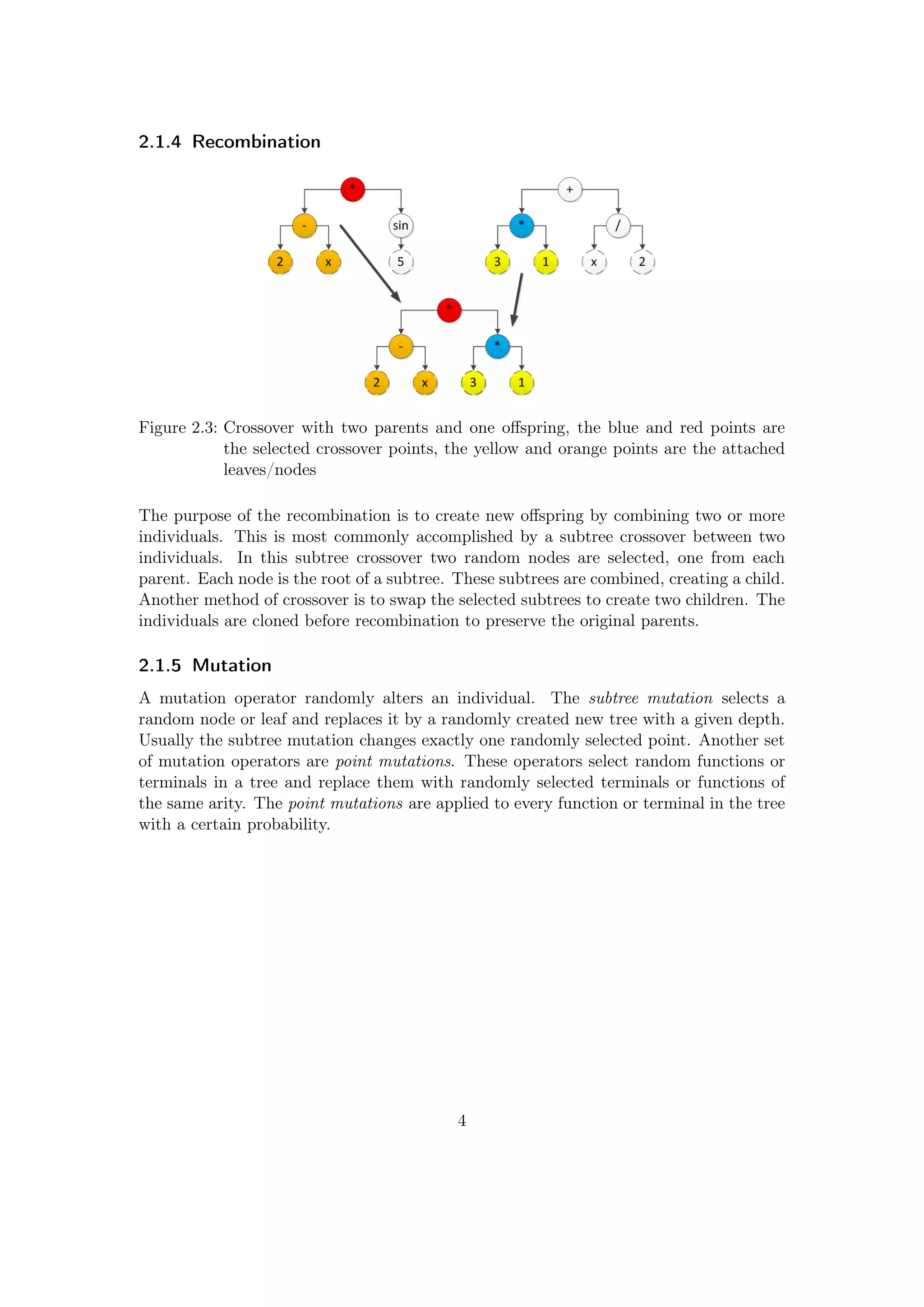
Figure 2.6: The probability for
choosing a crossover
point in the RGP
crossover
The crossover is performed with the winners of the
rank based selection. The crossover needs two par-
ents and selects a random crossover point from each
with a certain probability. The offspring is build
through combining the selected subtrees or termi-
nals. So with each crossover one child is created, as
shown in Figure 2.3. Each point has a probability
to be chosen when passed, the crossover probabil-
ity. If the point is not chosen, the tree is passed
further. The crossover works recursively similar to
the rand_expr_grow, therefore the probability for
a crossover point to get chosen is larger for points
situated higher in the tree. Figure 2.6 shows the
probability for each point to be directly chosen for
a crossover probability of 0.5 (50%). If no crossover
point is directly chosen, the last passed point is used
for the crossover.
The Listing 2.3 displays the pseudocode of the Crossover.
Listing 2.3: RGP: crossover
crossover ( expr1 , expr2 , cross_p )
newexpr1= expr1
i f is_node ( expr1 ) //no terminal
cross_idx= select_left_or_right_subtree ( expr1 )
i f rand () <= cross_p {
then
newexpr1 [ cross_idx ]= select_random_subtree ( expr2 , cross_p )
else
newexpr1 [ cross_idx ]= crossover ( expr1 [ cross_idx ] , expr2 , cross_p )
return newexpr1
14](https://image.slidesharecdn.com/7917a8af-6d0a-4b34-9fa4-99117e0f65d0-160111142603/75/Thesis-20-2048.jpg)
![expr1: the first parent, an individual
e.g., 10
expr2: the second parent, an individual
cross_p: probability for selecting a subtree for crossover, any value between
0 and 1. This value determines the probability to choose a crossover point
newexpr1: the child created by the crossover, an individual
2.3.5 Mutation
RGP uses different methods for altering an individual:
Insert Subtree
This mutation operator selects leaves by uniform random sampling and replaces them
with new created subtrees of a certain depth. Initially the total amount of leaves in the
tree is measured and a certain amount of leaves is selected by uniform random sampling.
Then all points in the tree are analyzed whether it is a node(function) or leaf(constant
or variable). If a leaf is found and matches one of the selected leaves, this leaf is replaced
by a new subtree of a given depth. This subtree is created by use of the full method. If
the current point is a node, the mutation is called recursively with each subtree of this
node. The pseudocode in Listing 2.4 shows the function insert_subtree.
Listing 2.4: RGP: insert subtree
insert_subtree ( expr , funcset , inset , conset , strength , sub_d)
no_of_leaves= count_leaves ( func )
no_of_samples= select_smaller ( strength , no_of_leaves )
s_leaves []= sample_wout_replace ( no_of_leaves , no_of_samples )
c_leaf= 0;
insert_subtree_r ( . . . )
insert_subtree_r ( expr , s_leaves [ ] , funcset , inset , conset , sub_d , c_leaf )
i f is_variable ( expr ) or is_constant ( expr )
then
c_leaf= c_leaf + 1
i f s_leaves [ ] c o n s i s t s c_leaf
then
expr= swap_with_new_tree ( funcset , inset , conset , sub_d)
else i f is_node ( expr )
then
for i=1 to a r i t y ( expr )
insert_subtree_r ( subtree_i ( expr ) , . . . )
15](https://image.slidesharecdn.com/7917a8af-6d0a-4b34-9fa4-99117e0f65d0-160111142603/75/Thesis-21-2048.jpg)
![expr: the expression tree altered by the mutation,
e.g., sin(x) + exp(x2) - x3 at begin, then certain subtrees or leaves
strength: max number of leaves to be altered
s_leaves[]: set of numbers of the selected leaves
c_leaf: current leaf
Delete Subtree
This mutation operator selects subtrees of a certain depth by uniform random sampling
and replaces them by a randomly selected terminal. First, the number of subtrees of an
user defined depth is measured. A set consisting of the current number for each subtree
is stored. Then a number of these subtrees, depending on the mutation strength, is
selected by uniform random sampling. Next the expression tree is analyzed. If a subtree
with matching depth is found and its number is in the set of the selected subtrees, it is
removed and replaced by a terminal. The pseudocode of delete_subtree is shown in
Listing 2.5.
Listing 2.5: RGP: delete subtree
delete_subtree ( expr , inset , conset , str , subtree_d , const_p )
no_subtree_match_d= count_matching_subs ( expr , subtree_d )
no_of_samples= select_smaller ( str , no_stree_match_d )
s_match_subtrees []= sample_wout_replace ( no_stree_match_d , no_of_samples )
c_matching_subtree= 0
delete_subtree_rec ( . . . )
delete_subtree_rec ( expr , c_m_stree , s_m_stres [ ] , subtree_d , conset , i n s e t )
i f is_node ( expr )
then
i f depth ( expr ) == subtree_d
then
c_m_stree= c_m_stree + 1
then
i f s_m_strees [ ] c o n s i s t s c_m_stree
then
i f rand () <= const_p
then
expr= new_constant ( conset )
else
expr= new_input_variable ( i n s e t )
for i=1 to a r i t y ( expr )
delete_subtree_rec ( subtree_i ( expr ) , . . . )
16](https://image.slidesharecdn.com/7917a8af-6d0a-4b34-9fa4-99117e0f65d0-160111142603/75/Thesis-22-2048.jpg)
![expr: the expression tree altered by the mutation,
e.g., sin(x) + exp(x2) - x3 at begin, then certain subtrees or leaves
str: max number of deleted subtrees
subtree_d: depth of subtrees to be deleted
s_m_stres[]: set of selected matching subtree numbers
c_m_stree: current depth matching subtree
Change Label
This mutation operator selects certain points in the tree by uniform random sampling
and alters them. First the total amount of mutation points is measured. A mutation
point is a node or leaf of the tree. Then certain mutation points are selected from this
amount by uniform random sampling. All points in the tree are analyzed whether they
are a node, constant or variable and if the current mutation point matches one of the
selected mutation points. Then the following actions are performed depending on the
type of the mutation point:
• for a constant, a uniform random value is added to this constant
• for a variable, this variable is replaced by another(maybe identical) variable from
the variable set
• for a node, the arity of the connected function is measured and a random function
is chosen from the function set. If the chosen function matches the arity of the old
function, the functions are swapped. If they do not match, the old function is used.
Also if the mutation point is a node, the change label mutator is called recursively
with each subtree.
The function is named change_label because it alters the labeling of a node oder leaf.
The Listing 2.6 shows the pseudocode of change_label, the parameters are:
expr: the expression tree altered by the mutation,
can be a node(function) or leaf(constant or variable)
strength: max number of altered points
sample_mps[]: set of selected mutation points
curren_mp: current mutation point
17](https://image.slidesharecdn.com/7917a8af-6d0a-4b34-9fa4-99117e0f65d0-160111142603/75/Thesis-23-2048.jpg)
![Listing 2.6: RGP: change label
change_label ( expr , funcset , inset , conset , strength )
no_of_mutation_points= func_size ( func )
no_of_samples= select_smaller ( strength , no_of_mutation_points )
sample_mps []= sample_wout_replace ( no_of_mutation_points , no_of_samples )
current_mp= 0
mutate_label ( expr , sample_mps [ ] , funcset , inset , current_mp )
mutate_label ( expr , sample_mps [ ] , funcset , inset , current_mp )
current_mp= current_mp + 1
i f is_variable ( expr )
then
i f sample_mps [ ] c o n s i s t s current_mp
then
expr= new_input_variable ( i n s e t )
else i f is_constant ( expr )
then
i f sample_mps [ ] c o n s i s t s current_mp
then
expr= actual_constant + rand ()
else i f is_node ( expr )
then
i f sample_mps [ ] c o n s i s t s current_mp
then
old_function= function_name ( expr )
arity_old_function= get_arity ( old_function )
new_function= get_random_function ( funcset )
i f a r i t y ( new_function ) == arity_old_function
then
expr= new_function
for i=1 to a r i t y ( expr )
mutate_label ( subtree_i ( expr ) , . . . )
18](https://image.slidesharecdn.com/7917a8af-6d0a-4b34-9fa4-99117e0f65d0-160111142603/75/Thesis-24-2048.jpg)
![2.3.6 Crossover and Mutation in the GP run
The crossover and mutation are applied after the selection. First a crossover is performed
with the two winner sets, then the children are mutated. The mutation function is
selected by uniform random sampling, so for each of the described mutation methods
there is a chance of 1/3(33.3%) to be used. This process is done twice to generate
enough mutated children to match the number of losers. The pseudocode of the GP run
where the functions are used is displayed in Listing 2.7:
Listing 2.7: RGP: crossover and mutation in the GP run
for i= 0 to i= length ( winnersA [ ] ) do
winner_childrenA [ i ]= mutatefunc ( crossover ( winnersA [ i ] , winnersB [ i ] ) )
for i= 0 to i= length ( winnersB ) do
winner_childrenB [ i ]= mutatefunc ( crossover ( winnersA [ i ] , winnersB [ i ] ) )
winner_children []= add ( winner_childrenA [ ] , winner_childrenB [ ] )
2.3.7 Extinction Prevention
This method is not used by default by RGP, but a similar method will be implemented
in C later on, therefore it is described here. It is used to prevent duplicate individuals
from occurring in the population. The winner children and the losers are combined to a
wl set. Then the amount of unique individuals in this wl set is measured. If it is equal
or greater than the amount of losers, the losers are replaced by the individuals in this
set. If not, a warning is send and the amount of missing individuals in the wl set is filled
with duplicates. The Listing 2.8 shows the pseudocode.
Listing 2.8: RGP: extinction prevention
e x t i n c t i o n _prevention ( winner_children [ ] , l o s e r s [ ] )
no_losers= length ( l o s e r s [ ] )
wl_children []= add ( winnerChildren [ ] , l o s e r s [ ] )
unique_wl_children []= unique ( wl_children [ ] )
no_unique_wl_children= length ( unique_wl_children [ ] )
i f no_unique_wl_children < no_losers
warning ( "not␣enough␣ unique ␣ i n d i v i d u a l s " )
no_missing= no_losers − no_unique_wl_children
for i= 1 to no_missing
replace [ i ]= wl_children [ i ]
unique_wl_children []= add ( unique_wl_children [ ] , replace [ ] )
for i= 1 to no_losers
unique_children [ i ]= unique_wl_children [ i ]
l o s e r s []= unique_children [ ]
winner_children[]: the set of the individuals created by the crossover
losers[] set of losers, sorted by the selection
19](https://image.slidesharecdn.com/7917a8af-6d0a-4b34-9fa4-99117e0f65d0-160111142603/75/Thesis-25-2048.jpg)

![3 Concept, Objectives and
Implementation
3.1 Concept for Accelerating RGP
The R environment is for some applications not the fastest system, as described in section
2.2.3. RGP uses many recursive functions and some loops, therefore the computation
speed is partially slow. In general, GP systems need a lot of computation time because
they have a giant search space. So this problem is particularly noticeable for experiments
with a large number of input variables and a large function set. These runs may take
from several hours to days to complete with a good result. This directly led to the
question how to improve the performance of the system. One idea was to have parallel
computation runs by using some package like Snow [24]. This has been implemented and
it greatly reduces the runtime for a set of runs, but a single run takes as long as before.
Another idea was to parallelize the functions itself, but this was much more complicated
to implement, therefore the idea was dropped for the time being. The actual used concept
is to overcome the typical problems of the R environment, the slow loops and overloaded
functions, by using the option of R to link and use C code.
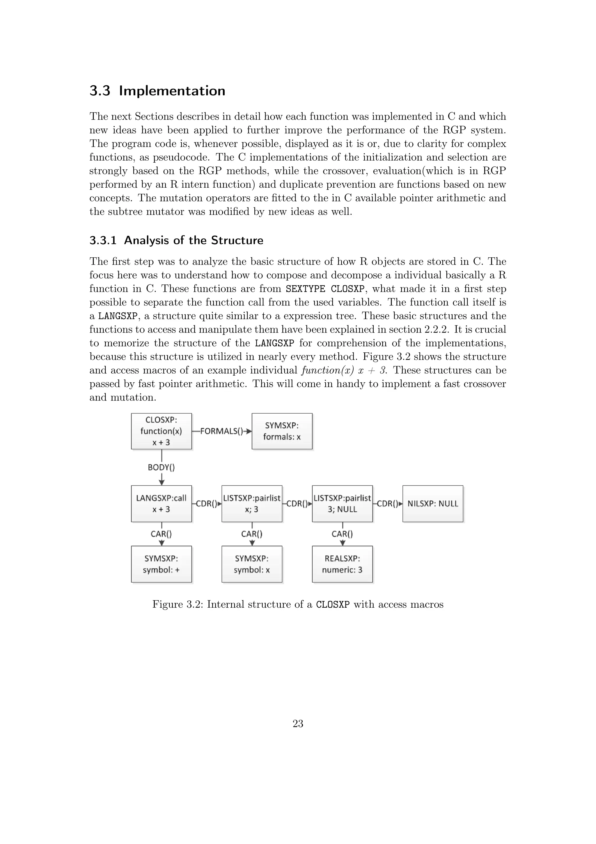
3.1.1 R code as Executable Specification for C Code
Figure 3.1: Concept for the RGP/C
implementation
The basic concept is to have C code which has ex-
actly the same functionality as the existing RGP
R Code. R code is quite easy to read and under-
stand and since the system is provided in R, it is
assumable that the users of RGP have a certain
knowledge of R, but not necessarily of C. The di-
rect manipulation of R objects in C is quite rarely
used and there is neither a good documentation
nor many people who have the required insight into
the R structures to do this. Therefore the concept
comes to two levels of RGP, one on the surface,
programmed in R, and one under the surface, im-
plemented in C.
This combines two main advantages:
• the speed of C functions
• the easy usability of the R environment
21](https://image.slidesharecdn.com/7917a8af-6d0a-4b34-9fa4-99117e0f65d0-160111142603/75/Thesis-27-2048.jpg)


![Listing 3.1: C: wrapper
SEXP randExprGrow (SEXP funcSet , SEXP inSet , SEXP maxDepth_ext ,
SEXP constProb_ext , SEXP subtreeProb_ext , SEXP constScaling_ext )
{
SEXP rfun ;
struct RandExprGrowContext TreeParams ; // s t r u c t u r e for s t o r i n g values
TreeParams . nFunctions= LENGTH( funcSet ) ; //number of functions
const char ∗ arrayOfFunctions [ TreeParams . nFunctions ] ;
int arrayOfArities [ TreeParams . nFunctions ] ;
TreeParams . a r i t i e s = arrayOfArities ;
// convert funcSet to chars
for ( int i= 0; i < TreeParams . nFunctions ; i++) {
arrayOfFunctions [ i ]= CHAR(STRING_ELT( funcSet , i ) ) ;
} // get the a r i t i e s of the functions
g e t A r i t i e s ( arrayOfFunctions , TreeParams . a r i t i e s , TreeParams . nFunctions ) ;
TreeParams . functions = arrayOfFunctions ;
// Variables
TreeParams . nVariables= LENGTH( inSet ) ;
const char ∗ arrayOfVariables [ TreeParams . nVariables ] ;
for ( int i= 0; i < TreeParams . nVariables ; i++) {
arrayOfVariables [ i ]= CHAR(STRING_ELT( inSet , i ) ) ;
}
TreeParams . v a r i a b l e s = arrayOfVariables ;
//maximal depth of tree
PROTECT(maxDepth_ext = coerceVector (maxDepth_ext , INTSXP ) ) ;
TreeParams . maxDepth= INTEGER(maxDepth_ext ) [ 0 ] ;
// constant prob
PROTECT( constProb_ext = coerceVector ( constProb_ext , REALSXP) ) ;
TreeParams . constProb= REAL( constProb_ext ) [ 0 ] ;
// subtree prob
PROTECT( subtreeProb_ext = coerceVector ( subtreeProb_ext , REALSXP) ) ;
TreeParams . probSubtree= REAL( subtreeProb_ext ) [ 0 ] ;
// constant s c a l i n g
PROTECT( constScaling_ext = coerceVector ( constScaling_ext , REALSXP) ) ;
TreeParams . constScaling= REAL( constScaling_ext ) [ 0 ] ;
int currentDepth= 0;
GetRNGstate ( ) ;
PROTECT( rfun= randExprGrowRecursive(&TreeParams , currentDepth ) ) ;
PutRNGstate ( ) ;
UNPROTECT( 5 ) ;
return rfun ;
}
3.3.4 Constant Creation and Scaling
The parameter constScaling_ext is a scaling factor used in the constant creation, nor-
mally the constants have a range[-1;1]. With this value this range can be adjusted. The
range is simply multiplied by the scaling factor. For example, the range would be [-5;5]
for a scaling factor of 5. In RGP this factor can be applied by defining a constant factory,
25](https://image.slidesharecdn.com/7917a8af-6d0a-4b34-9fa4-99117e0f65d0-160111142603/75/Thesis-31-2048.jpg)
![a function for generating constants. It has many advantages to have this kind of factor,
so it was directly implemented in the C code. The Listing 3.2 shows how a constant is
created in C.
Listing 3.2: C: random number creation
SEXP randomNumber(double constScaling ) {
SEXP Rval ;
PROTECT( Rval = allocVector (REALSXP, 1 ) ) ;
REAL( Rval ) [ 0 ] = constScaling ∗ (( unif_rand () ∗ 2) − 1 ) ;
UNPROTECT( 1 ) ;
return Rval ; }
26](https://image.slidesharecdn.com/7917a8af-6d0a-4b34-9fa4-99117e0f65d0-160111142603/75/Thesis-32-2048.jpg)
![3.3.5 Initialization
The first step was to implement a function to compose new individuals, which has the
same design and functionality as the rand_expr_grow in section 2.3.2. Since this function
should provide the exact same functionality as the one from RGP, the code is strongly
based on the pseudocode of the mentioned function. The C implementation is displayed
in Listing 3.3 and the transfer parameters are explained below.
Listing 3.3: C: random expression grow
SEXP randExprGrowRecursive ( struct RandExprGrowContext ∗ TreeParams ,
int currentDepth ) {
i f (( unif_rand () <= TreeParams−>probSubtree)&&(currentDepth <
TreeParams−>maxDepth ))
{
const int funIdx= randIndex ( TreeParams−>nFunctions ) ;
const int a r i t y= TreeParams−>a r i t i e s [ funIdx ] ;
SEXP expr ;
PROTECT( expr= R_NilValue ) ;
for ( int i =0; i < a r i t y ; i++ ) {
SEXP newParameter ;
PROTECT( newParameter = randExprGrowRecursive ( TreeParams ,
currentDepth +1));
PROTECT( expr= LCONS( newParameter , expr ) ) ;
}
PROTECT( expr= LCONS( i n s t a l l ( TreeParams−>functions [ funIdx ] ) , expr ) ) ;
UNPROTECT(2 + 2∗ a r i t y ) ;
return expr ;
}
else i f ( unif_rand () <= TreeParams−>constProb ){ // create constant
return randomNumber( TreeParams−>constScaling ) ;
} else {
const int varIdx= randIndex ( TreeParams−>nVariables ) ; // create v a r i a b l e
SEXP expr2 ;
PROTECT( expr2= i n s t a l l ( TreeParams−>v a r i a b l e s [ varIdx ] ) ) ;
UNPROTECT( 1 ) ;
return expr2 ;
}
}
// Create Population
SEXP createPopulation (SEXP popSize_ext , SEXP funcSet , SEXP inSet ,
SEXP maxDepth_ext , SEXP constProb_ext , SEXP subtreeProb_ext ,
SEXP constScaling_ext ) {
SEXP pop ;
PROTECT( popSize_ext = coerceVector ( popSize_ext , INTSXP ) ) ;
int popSize= INTEGER( popSize_ext ) [ 0 ] ;
PROTECT( pop= allocVector (VECSXP, popSize ) ) ;
for ( int i =0; i < popSize ; i++) {
SET_VECTOR_ELT(pop , i , randFuncGrow ( funcSet , inSet , maxDepth_ext ,
constProb_ext , subtreeProb_ext , constScaling_ext ) ) ; }
UNPROTECT( 2 ) ;
return pop ;
}
27](https://image.slidesharecdn.com/7917a8af-6d0a-4b34-9fa4-99117e0f65d0-160111142603/75/Thesis-33-2048.jpg)

![3.3.6 Selection
The selection is grounded on the RGP code displayed in Section 2.3.3. The only difference
is the sampling method. In RGP a unique sample without replacement for each rank
based selection is drawn, resulting in a probability for drawing the same individuals for
each ranking. For this implementation, one sample without replacement is drawn and
then divided. Thus it is ensured that both rank based selections are using different
individuals. The individuals themselves may be equal though. This fact is taken care of
in the duplicate prevention. The core of the selection is displayed in Listing 3.5.
Listing 3.5: C: Selection
GetRNGstate ( ) ;
snr ( sampleSize , ( popSize ) , y , x ) ;
PutRNGstate ( ) ;
for ( int i =0; i < ( sampleSize / 2) ; i++) {
sampleNumbersA [ i ]=y [ i ] ; }
for ( int i= ( sampleSize / 2) ; i < sampleSize ; i++) {
int j= i − ( sampleSize / 2 ) ;
sampleNumbersB [ j ]=y [ i ] ; }
PROTECT( rmseVectorA= allocVector (VECSXP, ( sampleSize / 2 ) ) ) ;
PROTECT( rmseVectorB= allocVector (VECSXP, ( sampleSize / 2 ) ) ) ;
for ( int i =0; i < ( sampleSize / 2) ; i++) {
SET_VECTOR_ELT( rmseVectorA , i ,
PROTECT( evalVectorizedRmse (VECTOR_ELT( population ,
( sampleNumbersA [ i ] −1)) , actualParameters , targetValues , bestRMSE ) ) ) ;
SET_VECTOR_ELT( rmseVectorB , i ,
PROTECT( evalVectorizedRmse (VECTOR_ELT( population ,
( sampleNumbersB [ i ] −1)) , actualParameters , targetValues , bestRMSE ) ) ) ;
UNPROTECT( 2 ) ; }
int ∗sortedNumbersA= Calloc (( sampleSize /2)∗ sizeof ( int ) , int ) ;
int ∗sortedNumbersB= Calloc (( sampleSize /2)∗ sizeof ( int ) , int ) ;
double ∗sortedRMSEA= Calloc (( sampleSize /2)∗ sizeof (double ) , double ) ;
double ∗sortedRMSEB= Calloc (( sampleSize /2)∗ sizeof (double ) , double ) ;
sortByRmse ( sampleNumbersA , sortedNumbersA , ( sampleSize /2) ,
rmseVectorA , sortedRMSEA ) ;
sortByRmse ( sampleNumbersB , sortedNumbersB , ( sampleSize /2) ,
rmseVectorB , sortedRMSEB ) ;
29](https://image.slidesharecdn.com/7917a8af-6d0a-4b34-9fa4-99117e0f65d0-160111142603/75/Thesis-35-2048.jpg)
![3.3.7 Evaluation
Figure 3.3: Addition tree
The evaluation is the critical element in the evolu-
tion run since it uses most of the computation time.
This behavior can easily be explained: e.g., for a re-
ally small individual shown in 3.3 with seven nodes
with the function "+", only variables as leaves with
an input vector of, e.g., 500 parameters for each
variable, the number of additions needed would
sum up to 500*7= 3500. For a selection size of 20
and only this kind of individuals this would result
in 70.000 additions for each evolution step. This value scales linear with the number
of nodes, number of input parameters and the selection size. Thus a new specialized
evaluator was designed to have a great impact on the overall performance of the system.
In an first attempt a new evaluator was designed which worked in a loop. After some
experiments it was obvious that the internal R evaluator was faster for greater numbers
of input parameters. This loop-evaluator had the big disadvantage, that for every differ-
ent input parameter value the whole tree had to be analyzed.
In a second attempt this evaluator was redesigned. The basic structure of the loop-
evaluator to analyze the trees was inherited, but the operations themselves were vector-
ized. So an individual tree needs to be analyzed only once.
In a third step this vectorized evaluator was improved by Olaf Mersmann and Oliver
Flasch by the use of the m4 macro package [1] to work more efficiently and support a
greater set of functions.
The vectorized evaluator returns a RMSE value, which is calculated in the wrapper
of the function. The code of the function itself is quite complex ( »1000 lines of code),
therefore only the basic pseudocode for a small set of functions is displayed in Listing 3.6.
Code Description:
To understand how the functions are analyzed, a quick look at the structure (Sec-
tion 3.3.1) is adjuvant. The function tree is passed and if a leaf (constant or
variable) is found the result vector is either filled with the constant or the with
the values of the related variable. If a node is found, the function symbol will be
compared with a hard coded set of functions. If it is a match and got the arity of
two, the proper arithmetic operation is performed with the resulting vector of both
subtrees. If the function has a arity of one, only the left subtree is used(as there is
no right one). If a function or variable is not in the related function/variable set,
an error is returned and the evaluation is terminated.
30](https://image.slidesharecdn.com/7917a8af-6d0a-4b34-9fa4-99117e0f65d0-160111142603/75/Thesis-36-2048.jpg)
![Listing 3.6: C: evaluator
void eval_vectorized ( expr , no_samples , i n s e t [ ] , params [ ] , no_vars , ∗ r e s u l t )
i f is_constant ( expr )
then
for i = 0 to i < no_samples
r e s u l t [ i ] = numeric_value ( expr )
return
else i f is_variable ( expr )
then
for i=0 to i < no_vars
i f expr == i n s e t [ i ]
then
for int j = 0 to j < no_samples
r e s u l t [ i ] = params [ i ∗ samples + j ]
return
else i f is_node ( expr )
then
func_sym= function_symbol ( expr )
i f func_sym == "+"
new l e f t _ r e s u l t [ no_samples ]
new right_result [ no_samples ]
eval_vectorized ( left_subtree , . . . , l e f t _ r e s u l t [ ] )
eval_vectorized ( right_subtree , . . . , right_result [ ] )
for i = 0 to i < no_samples
r e s u l t [ i ] = l e f t _ r e s u l t [ i ] + right_result [ i ] ;
return
else i f func_sym == "∗"
new l e f t _ r e s u l t [ no_samples ]
new right_result [ no_samples ]
eval_vectorized ( left_subtree , . . . , l e f t _ r e s u l t [ ] )
eval_vectorized ( right_subtree , . . . , right_result [ ] )
for i = 0 to i < no_samples
r e s u l t [ i ] = l e f t _ r e s u l t [ i ] ∗ right_result [ i ] ;
return
else i f func_sym == " sin "
then
new l e f t _ r e s u l t [ no_samples ]
eval_vectorized ( left_subtree , . . . , l e f t _ r e s u l t [ ] )
for i = 0 to i < no_samples
r e s u l t [ i ] = sin ( l e f t _ r e s u l t [ i ] )
return
else
e r r o r ()
no_samples: size of parameter vector per input variable
params[] input variable parameter vector
no_vars: number of different variables in inset
31](https://image.slidesharecdn.com/7917a8af-6d0a-4b34-9fa4-99117e0f65d0-160111142603/75/Thesis-37-2048.jpg)
![3.3.8 Duplicate Prevention
The duplicate prevention is a development introduced to the C implementation, seizing
the basic concept behind the extinct prevention (Section 2.3.7). The reason is as follows:
If the populations approaches a local optimum and the best RMSE value does not change
for many evolution steps, the best individual can dominate the whole population.1 In
the end, only equal individuals are selected for the crossover, leading to very similar
children and thus less variation. In a standard GP run, the winners themselves are never
changed. To prevent individuals from dominating the population, the idea is to identify
individuals with equal fitness in the winner population and to replace or alter them before
the crossover takes place. This function has therefore two effects: the winners can be
modified(with exception of the best individual), this can lead to a better fitting of the
problem. Furthermore the winners can be replaced by completely new individuals. This
greatly rises the variety of the population, especially due to the fact that this operation
is performed before the crossover.
Code Description:
After the selection, the RMSE values of the winner sets are compared against each
other, if they have the same RMSE value, the duplicate individuals from winner
set A are replaced by new grown trees. The duplicate individuals of winner set B
are modified by a random mutation operator.
Listing 3.7: C: duplicate prevention
for ( int i =0; i < (( sampleSize /4) −1); i++) {
i f (sortedRMSEA [ i ] == sortedRMSEA [ i +1]) {
SET_VECTOR_ELT( population , sortedNumbersA [ i +1] − 1 ,
randFuncGrow ( funcSet , inSet , maxDepth_ext , constProb_ext ,
subtreeProb_ext , constScaling_ext ) ) ;
}}
for ( int i =0; i < (( sampleSize /4) −1); i++) {
i f (sortedRMSEB [ i ] == sortedRMSEB [ i +1]) {
SET_VECTOR_ELT( population , sortedNumbersB [ i +1] − 1 ,
PROTECT( deleteInsertChangeSubtree (VECTOR_ELT( population ,
sortedNumbersB [ i +1] − 1) , funcSet , inSet , constProb_ext , subtreeProb_ext ,
maxDepth_ext , maxLeafs_ext , maxNodes_ext , constScaling_ext ) ) ) ;
UNPROTECT( 1 ) ; }}
1
this is caused by the steady state rank-based selection
32](https://image.slidesharecdn.com/7917a8af-6d0a-4b34-9fa4-99117e0f65d0-160111142603/75/Thesis-38-2048.jpg)
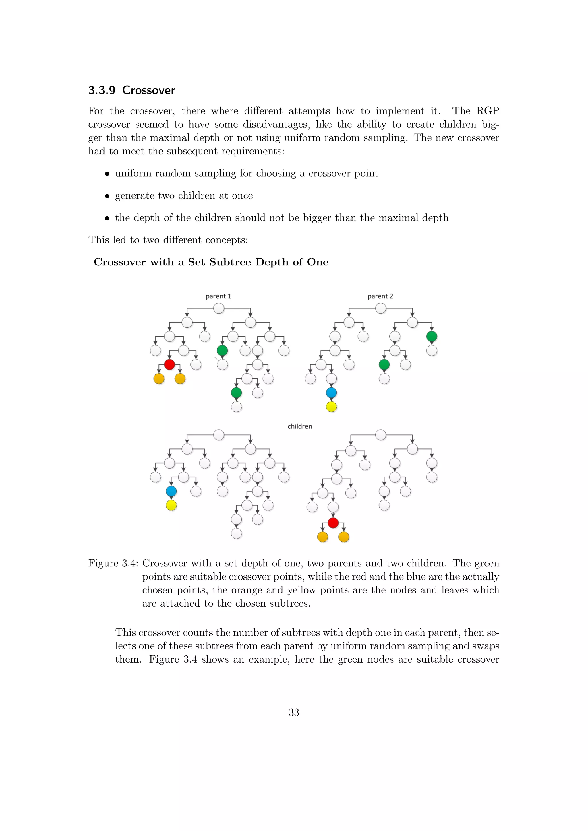
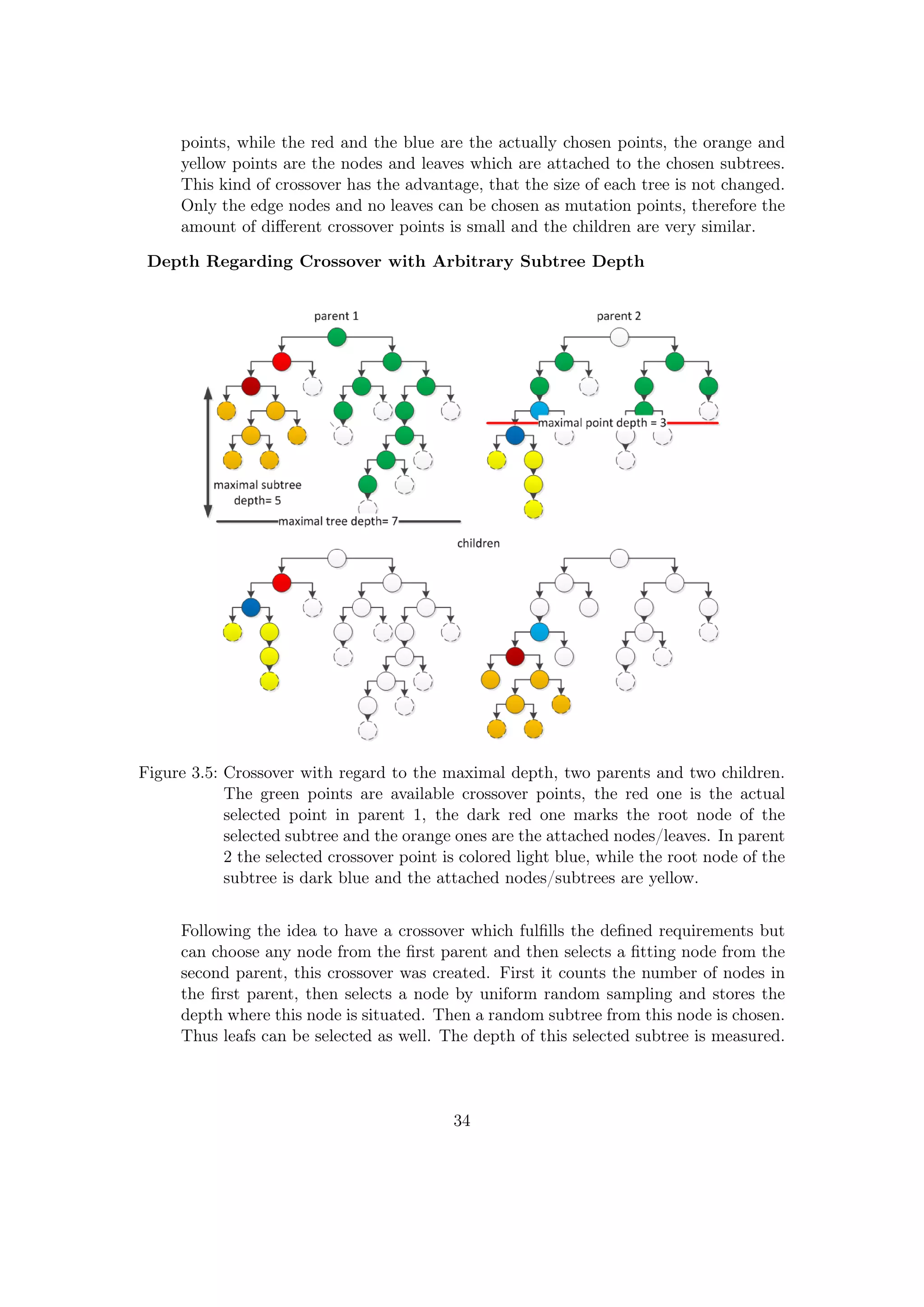


![Mutate Nodes
The mutate_nodes function works similar to the mutate_leaves with the difference that
it changes nodes. Every node in a tree is changed by a certain probability and the node
function is replaced by a function of the same arity. The swapping process itself is the
main difference to the original change_label mutator (Section 2.3.5) since it selects a
random function from the function set until a matching one with the same arity is found.
Listing 3.11 shows the C code. The struct RandExprGrowContext * TreeParams is part
of the initialization and explained in Section 3.3.5.
Listing 3.11: C: mutate nodes
void changeNodesRecursive (SEXP rExpr ,
struct RandExprGrowContext∗ TreeParams ) {
i f ( isNumeric ( rExpr )) {
return ;
} else i f ( isSymbol ( rExpr )) {
return ;
} else i f (( isLanguage ( rExpr )) && ( unif_rand () <= 0 . 3 ) ) {
int oldArity= expression_arity ( rExpr ) ;
SEXP replacement ;
int arity , funIdx ;
while ( a r i t y != oldArity ) {
funIdx= randIndex2 ( TreeParams−>nFunctions ) ;
a r i t y= TreeParams−>a r i t i e s [ funIdx ] ;
}
PROTECT( replacement= i n s t a l l ( TreeParams−>functions [ funIdx ] ) ) ;
SETCAR( rExpr , replacement ) ;
UNPROTECT( 1 ) ;
}
changeNodesRekursive (CADR( rExpr ) , TreeParams ) ;
i f ( ! i s N u l l (CADDR( rExpr ) )) { // for functions with a r i t y one , e . g . , sin ()
changeNodesRekursive (CADDR( rExpr ) , TreeParams ) ; }
}
38](https://image.slidesharecdn.com/7917a8af-6d0a-4b34-9fa4-99117e0f65d0-160111142603/75/Thesis-44-2048.jpg)
![Remove Subtree
The function remove_subtree is again strongly based on the original R function(Section
2.3.5). It analyzes the tree and counts the subtrees with the depth of one. Then one of
these subtrees is selected by uniform sampling, removed and replaced by a constant or
variable. The Listing 3.12 displays the core of the C function.
Listing 3.12: C: remove subtree
void removeSubtreeRecursive (SEXP rExpr ,
struct deleteSubtreeContext ∗delSubCon , int ∗ counter ) {
SEXP replacement ;
i f ( isNumeric ( rExpr )) { // numeric constant . . .
return ; // nothing to do
} else i f ( isSymbol ( rExpr )) { //
return ; // nothing to do
} else i f ( isLanguage ( rExpr )) {// composite . . .
for (SEXP c h i l d = CDR( rExpr ) ; ! i s N u l l ( c h i l d ) ; c h i l d = CDR( c h i l d )) {
i f ( isLanguage (CAR( c h i l d )) ) {
i f ( ! isLanguage (CADR(CAR( c h i l d ) ) ) &&
! isLanguage (CADDR(CAR( c h i l d ) ) ) ) {
∗ counter= ∗ counter + 1;
i f (∗ counter == delSubCon−>rSubtree ) {// s e l e c t e d subtree found
i f ( unif_rand () <= delSubCon−>constProb ) {
replacement= allocVector (REALSXP, 1 ) ;
REAL( replacement )[0]= delSubCon−>constScaling ∗
(( unif_rand () ∗ 2) − 1 ) ;
} else {
int varIdx= randIndex ( delSubCon−>nVariables ) ;
replacement= i n s t a l l ( delSubCon−>v a r i a b l e s [ varIdx ] ) ;
}
SETCAR( child , replacement ) ;
}}}}
i f (∗ counter <= delSubCon−>rSubtree ) {
removeSubtreeRecursive (CADR( rExpr ) , delSubCon , counter ) ;
i f ( ! i s N u l l (CADDR( rExpr ) )) { // for functions with a r i t y one e . g sin ()
removeSubtreeRecursive (CADDR( rExpr ) , delSubCon , counter ) ;
}}}}
deleteSubtreeContext *delSubCon
A special struct created and filled in the wrapper of remove subtree. It contains
the input variable set, the number of input variables, the constant probability and
scaling value, the subtree counter and the selected subtree number.
39](https://image.slidesharecdn.com/7917a8af-6d0a-4b34-9fa4-99117e0f65d0-160111142603/75/Thesis-45-2048.jpg)
![Insert Subtree
The C implementation of the insert_subtree mutator comprises some additional ideas.
The basic structure is again strongly based on the original function(Section 2.3.5), thus
this mutation operator basically counts the leaves in a tree and replaces one uniformly
chosen by a subtree of depth one. For the C mutation operator is was thought to be
advantageous to add a soft restart criterion: The amount of leaves and nodes and com-
pared with a user defined maximal number of nodes/leaves. If this number is matched,
the tree is recognized as oversized and replaced by a new grown tree. This effectively
restricts the maximal size of the trees in the population and adds some variation. It also
replaces very small trees with only one leaf and a depth of zero. Since this mutator is
not the optimal place for a complexity measurement, this function is to be moved into
the selection process later on. As the code of this function is again quite large, only a
part of the in this case more interesting wrapper is illustrated in Listing 3.13.
Listing 3.13: C: insert subtree
SEXP insertSubtree (SEXP rFunc , SEXP funcSet , SEXP inSet ,
SEXP constProb_ext , SEXP subtreeProb_ext , SEXP maxDepth_ext ,
SEXP maxLeafs_ext , SEXP maxNodes_ext , SEXP constScaling_ext ) {
// i n i t TreeParams , convert S−o b j e c t s
. . .
countLeafs (BODY( rFunc ) , &leafCounter ) ;
countNodes (BODY( rFunc ) , &nodeCounter ) ;
// Rprintf (" %d" , nodeCounter ) ;
// depth= countDepth (BODY( rFunc ) , depth ) ;
// Rprintf (" depth %d" , depth ) ;
i f (( leafCounter > 1) && ( leafCounter <= maxLeafs)&&
( nodeCounter <= maxNodes )) {
GetRNGstate ( ) ;
rLeaf= rand_number( leafCounter ) ;
insertSubtreeRecursive (BODY( rFunc ) , &TreeParams ,& counter , rLeaf , depth ) ;
PutRNGstate ( ) ; //Todo Else for symbols and constants
} else { // r e s t a r t i f t r e e s get too big or small
SEXP rExpr ;
PROTECT( subtreeProb_ext = coerceVector ( subtreeProb_ext , REALSXP) ) ;
TreeParams . probSubtree= REAL( subtreeProb_ext ) [ 0 ] ;
GetRNGstate ( ) ;
PROTECT( rExpr= randExprGrowRecursive(&TreeParams , 1 ) ) ;
PutRNGstate ( ) ;
SET_BODY( rFunc , rExpr ) ;
UNPROTECT( 2 ) ;
}
UNPROTECT( 5 ) ;
return rFunc ;
40](https://image.slidesharecdn.com/7917a8af-6d0a-4b34-9fa4-99117e0f65d0-160111142603/75/Thesis-46-2048.jpg)

![maxleaves and maxnodes
restart criterion used in the insert subtree mutator, if a tree got equal or more
leaves/nodes it is replaced by a new one
constprob
probability for generating a constant in all tree growing functions
constscaling
scaling factor for the constants, normally they have the range [-1,1], this range is
multiplied by this factor
subtreeprob
probability for creating a subtree in all tree growing functions
rmselimit
stop criterion, if set to a value greater than zeroï¿1
2, the run is stopped if this value
is smaller or equal the best reached RMSE. For zero it is disabled
returnrmse
if set to zero, the population is returned after the evolution is stopped, for one the
reached best RMSE.
silent
if set to one, all outputs are stopped, if zero the system continuously displays the
step number, reached best RMSE and runtime in seconds
timelimit
stop criterion, if set to a value greater zero, the run is stopped after a given time
in seconds. For zero it is disabled
43](https://image.slidesharecdn.com/7917a8af-6d0a-4b34-9fa4-99117e0f65d0-160111142603/75/Thesis-49-2048.jpg)
![4 Experiments
The experiments were designed to prove the acceleration and performance. Also a com-
parison with DataModeler [7] is done to rank the overall performance of the system
in comparison to a well-established GP system. DataModeler is a state-of-the-art GP
system in the mathematica environment for symbolic regression.
In detail the experiments cover:
• Unit tests of the initialization, evaluation and mutation
• A performance comparison between the GP evaluation runs of RGP and the C
implementation with a set of one and two dimensional problems
• Parameter tuning of the C GP system
• A comparison between the C implementation and DataModeler
The unit tests and the performance comparison between RGP and the C implementation
were performed on a Core i5 2500k with 8G of ram. The comparison with DataModeler
is done on a Core 2 Duo P8600 with 4G of RAM. The initialization, evaluation and
mutation are compared in terms of computation speed. The computation speed is defined
by CPU time each function uses to execute. The CPU time was measured by the internal
R system.time() function which returns the user time, system time and total elapsed
time. The user time is the CPU time charged for the execution of user instructions of
the calling process, therefore it will be used here.[22]
44](https://image.slidesharecdn.com/7917a8af-6d0a-4b34-9fa4-99117e0f65d0-160111142603/75/Thesis-50-2048.jpg)
![4.1 Unit tests
4.1.1 Initialization: Growing Full Trees
In this test the initialization of RGP and the C implementation were compared in terms
of computation speed. To get a good insight into the behavior of the functions, they
were parametrized to build exact the same trees. The full function was used, thus the
subtree probability was one. The function set was set to the basic functions with the
arity of two( +, -, *, /) . This was done to have a fixed amount of nodes and leaves in a
tree for a given depth. These amounts can be calculated by
• sum of nodes and leaves: n = 2depth+1 − 1
• number of leaves: 2depth
• number of nodes:
n
2
The experiments were performed in the ranges [0;12] for the tree depth and [10;100000]
for ntrees, the number of created trees. The computation time was measured in seconds
by steps of 10 milliseconds. Listing 4.1 shows the R code for the benchmark functions
and the used input parameters.
Listing 4.1: Experiments: growing random trees
functionSet <− functionSet ( "+" , "−" , "∗" , "/" )
inputVariableSet <− inputVariableSet ( "x" )
numericConstantSet <− constantFactorySet ( function () r u n i f (1 , −1, 1))
RGPGrowTrees <− function ( depth , number) {
for ( i in 1: number){
randExprGrow ( functionSet , inputVariableSet , numericConstantSet ,
subtreeprob = 1 , maxdepth = depth , constprob= 0.2 , curdepth= 0)
}}
benchRGPtree <− function ( depth , number) {
time <− system . time (RGPGrowTrees( depth , number ))
// return f i r s t element of time object , the time used by t h i s process
return time [ [ 1 ] ] }
CfuncSet= c ( "+" , "−" , "∗" , "/" )
CinSet= c ( "x" )
CGrowTrees <− function ( depth , number) {
for ( i in 1: number){
. Call ( "randExprGrow" , CfuncSet , CinSet , maxdepth= depth ,
constprob= 0.2 , subtreeprob= 1 , c o n s t s c a l i n g= 1)
}}
benchCtree <− function ( depth , number) {
time <− system . time ( CGrowTrees ( depth , number ))
return time [ [ 1 ] ] }
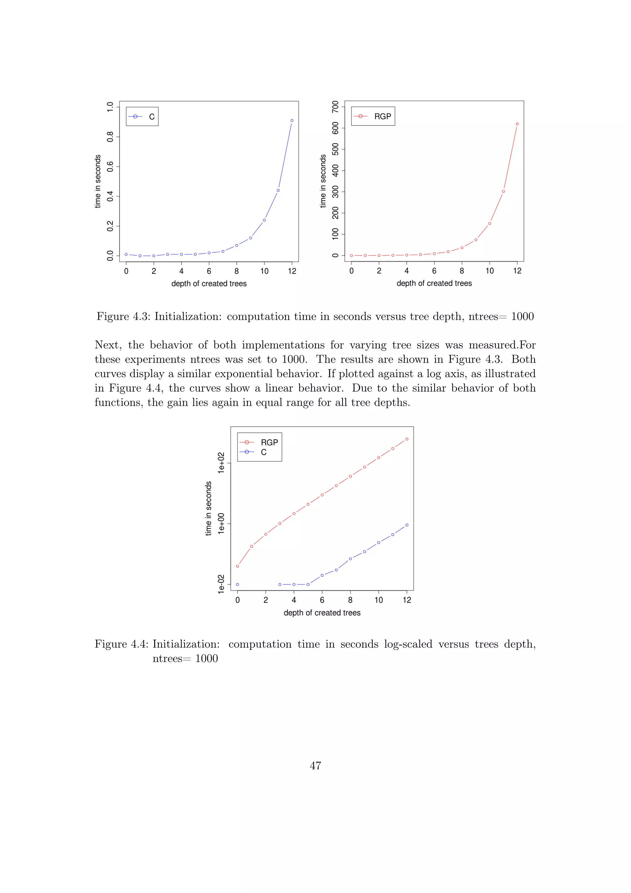
45](https://image.slidesharecdn.com/7917a8af-6d0a-4b34-9fa4-99117e0f65d0-160111142603/75/Thesis-51-2048.jpg)
![Figure 4.1: Initialization: computation time in seconds versus ntrees,tree depth= 7
Figure 4.1 displays the computation time vs ntrees for a set tree depth of 7. The course
of the curves shows for both implementations a linear behavior, the C implementation
curve has some variance. The gain of computation speed can easily be seen if plotting
both curves together against a log-scaled time axis, as done in Figure 4.2. The gain lies
in the range [1.e+2;1.e+3], e.g., for 10000 trees the speed gain is 538.
Figure 4.2: Initialization: computation time in seconds log-scaled versus ntrees,
tree depth= 7
46](https://image.slidesharecdn.com/7917a8af-6d0a-4b34-9fa4-99117e0f65d0-160111142603/75/Thesis-52-2048.jpg)

![speed_gain ≈
cRGP
cC
= 553.
Note that is is a rough approximation, since for greater tree sizes the speed gain gets
even higher. For a tree depth of 11, the cRGP is 7.6e-5 and cC is 11.8e-8 , therefore the
speed gain is 644.
4.1.2 Evaluation
The basic functionality of the C evaluation was already ensured during the development.
Therefore it calculates exactly the same as the internal R eval() function. For this test,
the behavior for boundary values was analyzed in a first step, then computation time
benchmarks were executed. Then different benchmark tests were performed to compare
the computation time of the R eval() used by RGP and the C evaluation function. The
setup for this tests was:
• 1000 randomly fully grown trees with the complete function set +, -, *, /, sin, cos,
tan, exp, log, sqrt, abs
• different input vector sizes in the range [10;1.e+6]
• different tree depths in the range [2;10]
The computation time was measured in seconds by steps of 10 milliseconds.
Boundary Values
Next, the behavior of the C evaluation function for boundary values was tested. This
was done for the functions with critical behavior for some values, i.e., /, tan, log, sqrt.
The C code is compiled by the GCC, which uses the IEEE 754 floating point numbers
and therefore supports the values INF(infinity) and NaN(Not a Number). These values
are returned for some boundary values in certain functions, in detail:
• x / 0 division by zero, e.g., f(x)= x / 0 returns INF for positive x values and -INF
for negative values of x
• tan(x) has the same behavior for values where cos(x)= 0 (
π
2
,
3π
2
,...), it returns INF
or -INF
• log(x) for a x value of zero it returns -INF, for negative x values NaNs are returned
• sqrt(x) for negative x values, NaNs are returned
Positive or negative INF values are no problem, they have just an infinite high RMSE
and are eliminated in the selection. NaNs cause problems in the selection, therefore they
are identified and replaced by very high RMSE values to have them eliminated by the
selection. These replacements are done in the wrapper of the evaluation function, where
the RMSE values are calculated.
49](https://image.slidesharecdn.com/7917a8af-6d0a-4b34-9fa4-99117e0f65d0-160111142603/75/Thesis-55-2048.jpg)
![R Benchmark Code
Listing 4.2 shows the R functions used for this comparison.
Listing 4.2: Experiments: evaluation
CfuncSet= c ( "+" , "∗" , "−" , "/" , "exp" , " sin " , " cos " , "tan" , " sqrt " , " log " , "abs" )
CinSet= c ( "x1" )
pop1 <− . Call ( " createPopulation " ,1000 , CfuncSet , CinSet ,
maxdepth= 4 , constprob= 0.2 , subtreeprob= 1 , s c a l i n g =1)
evalC <− function (x) {
for ( i in 1: length ( pop1 )) {
. Call ( " evalVectorized " , pop1 [ [ i ] ] , x) }
}
evalRGP <− function (x) {
for ( i in 1: length ( pop1 )) {
pop1 [ [ i ] ] ( x) }
}
benchEvalRGP <− function (x) {
time <− system . time (evalRGP ( 1 : x ))
time [ [ 1 ] ] // f i r s t element of time object , the time used by t h i s process
}
benchEvalC <− function (x) {
time <− system . time ( evalC ( 1 : x ))
time [ [ 1 ] ]
}
50](https://image.slidesharecdn.com/7917a8af-6d0a-4b34-9fa4-99117e0f65d0-160111142603/75/Thesis-56-2048.jpg)
![Computation Speed Comparison
Figure 4.6: RGP and C, computation time in seconds versus size of input vector,
tree depth= 6, N= 1000
Figure 4.6 shows a comparison of computation time for both evaluation functions for a
set population size of N= 1000 and a tree depth of 6 in the range [10;10000]. Both curves
have an linear behavior, the slope is slightly higher for the R eval() function. The gain
is initially high, due to the small computation time values of the C implementation, and
then becomes lower.
Table 4.2: Evaluation: speed gain vs depth and input vector size
Tree Depth
2 4 6 8 10
Vector Size Gain
10 NA 5 12 23 24.5
100 2 3 5 5 5.5
1000 1.2 1.53 1.66 1.72 1.79
10000 1.11 1.23 1.27 1.31 1.33
1.e+5 1.07 1.22 1.27 1.41 1.47
1.e+6 0.99 1.14 1.2 1.15 1.18
Table 4.2 shows the speed gain vs depth and input vector size. The value for tree
depth 2 and vector size 10 is NA, because the measured computation time was below 10
51](https://image.slidesharecdn.com/7917a8af-6d0a-4b34-9fa4-99117e0f65d0-160111142603/75/Thesis-57-2048.jpg)

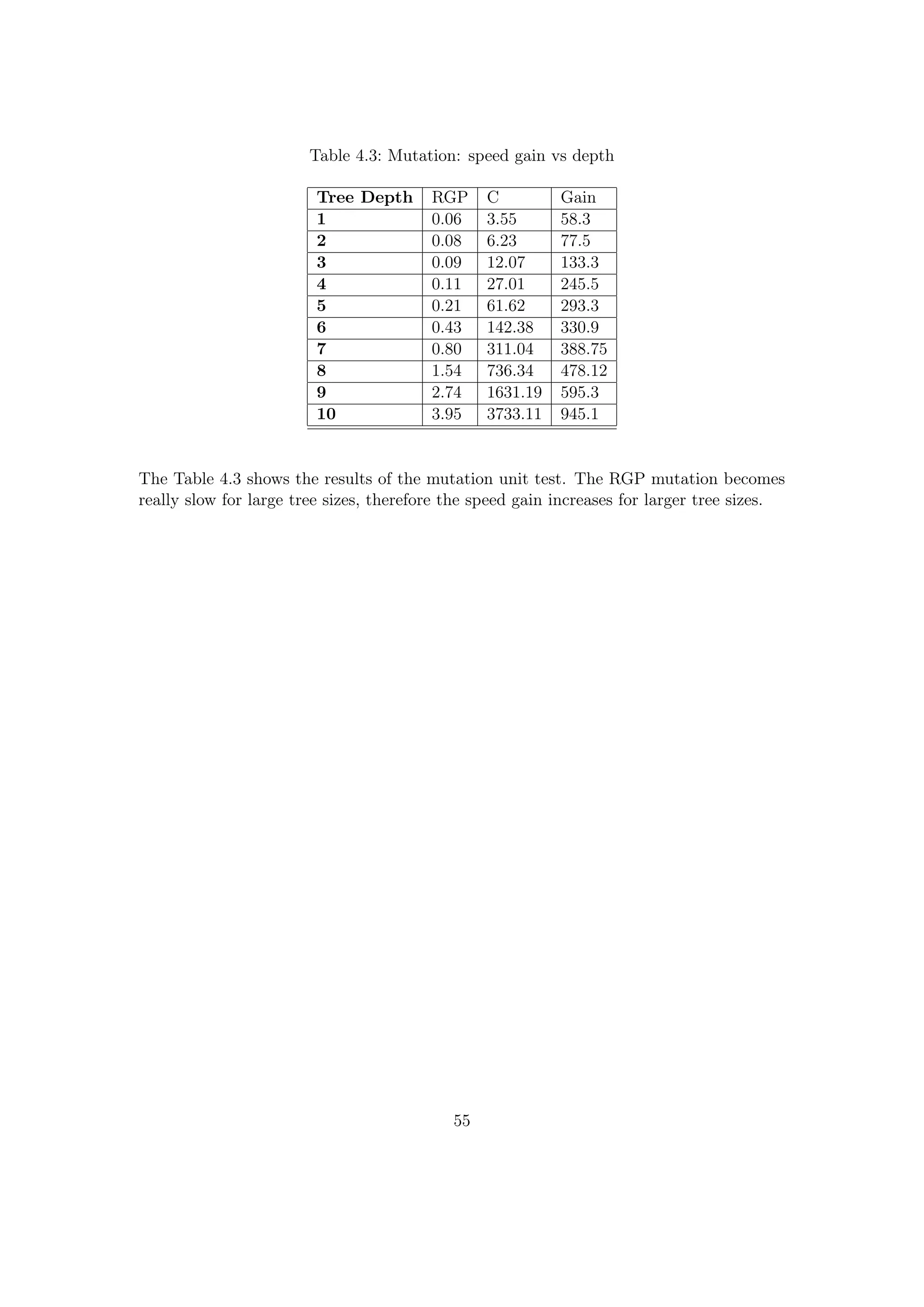
![4.1.3 Mutation
Some of the mutation operators are different for the RGP and the C implementation and
they use the random tree grow function, therefore a unit test is complicated. Thus in
this test, the insert and delete mutation operators, which are very similar, are compared.
The mutation changes the population, therefore for each comparison a new population
had to be generated. To control the number of nodes in the trees and minimize the
variation, the basic function set with functions of arity two and full grown trees were
used. Thus the equations for the number of nodes or leaves introduced in Section 4.1.1
can be applied. The population size was set to N=10000 to further reduce the effective
variation in the different populations.
The detailed test setup was:
• population: N= 10000, full grown trees
• tree depth range: [1;10]
• function set: +,-,*,/
Listing 4.3: Experiments: mutation
funcSet= c ( "+" , "∗" , "−" , "/" ,)
inSet= c ( "x" )
cmut <− function ( depth ) {
pop1 <− . Call ( " createPopulation " ,10000 , funcSet , inSet ,
maxdepth= depth , constprob= 0.2 , subtreeprob= 1 , s c a l i n g =1)
time <− system . time ( for ( i in 1: length ( pop1 )) {
CmutateDeleteInsert ( pop1 [ [ i ] ] ) } , gcFirst = TRUE)
time [ [ 1 ] ]
}
rgpmut <− function ( depth ) {
pop1 <− . Call ( " createPopulation " ,10000 , funcSet , inSet ,
maxdepth= depth , constprob= 0.2 , subtreeprob= 1 , s c a l i n g =1)
time <− system . time ( for ( i in 1: length ( pop1 )) {
RGPmutateDeleteInsert ( pop1 [ [ i ] ] ) } , gcFirst = TRUE)
time [ [ 1 ] ]
}
53](https://image.slidesharecdn.com/7917a8af-6d0a-4b34-9fa4-99117e0f65d0-160111142603/75/Thesis-59-2048.jpg)
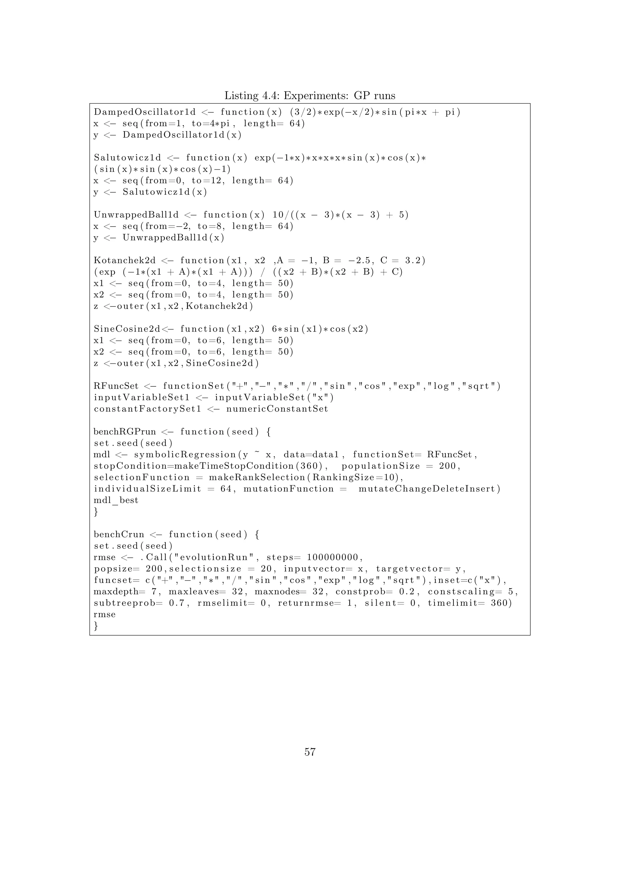
![4.2.1 Test Setup One-Dimensional Problems
Figure 4.2.1 displays the used one-dimensional functions.
(a) Damped Oscillator (b) Salustowicz (c) Unwrapped Ball
Figure 4.11: GP run: One dimensional problem set
Damped Oscillator function:
f(x) =
3
2
× exp (
−x
2
) × sin (π × x + π)
64 equidistant samples the range [1;4π]
Salustowicz function:
f(x) = exp(−x) × x3 sin(x) × cos(x) × (sin(x)2 × cos(x) − 1)
64 equidistant samples in the range [0;12]
Unwrapped Ball function:
f(x) =
10
(x − 3) × (x − 3) + 5
64 equidistant samples in the range[-2;8]
58](https://image.slidesharecdn.com/7917a8af-6d0a-4b34-9fa4-99117e0f65d0-160111142603/75/Thesis-64-2048.jpg)
![4.2.2 Test Setup Two-Dimensional Problems
Figure 4.12 displays the used two-dimensional functions.
(a) Kotanchek (b) SinusCosinus
Figure 4.12: GP run: Problem set 2d
Kotanchek function:
f(x) =
exp −(x1 − 1)2
(x2 − 2.5)2 + 3.2
x1, x2 range:[0;4] 50 equidistant samples each
input vector size: 50 × 50 = 2500 points for each variable
SinusCosinus function:
f(x) = 6 × sin(x1) × cos(x2)
x1, x2 range:[0;6] 50 equidistant samples each
input vector size: 50 × 50 = 2500 points for each variable
59](https://image.slidesharecdn.com/7917a8af-6d0a-4b34-9fa4-99117e0f65d0-160111142603/75/Thesis-65-2048.jpg)

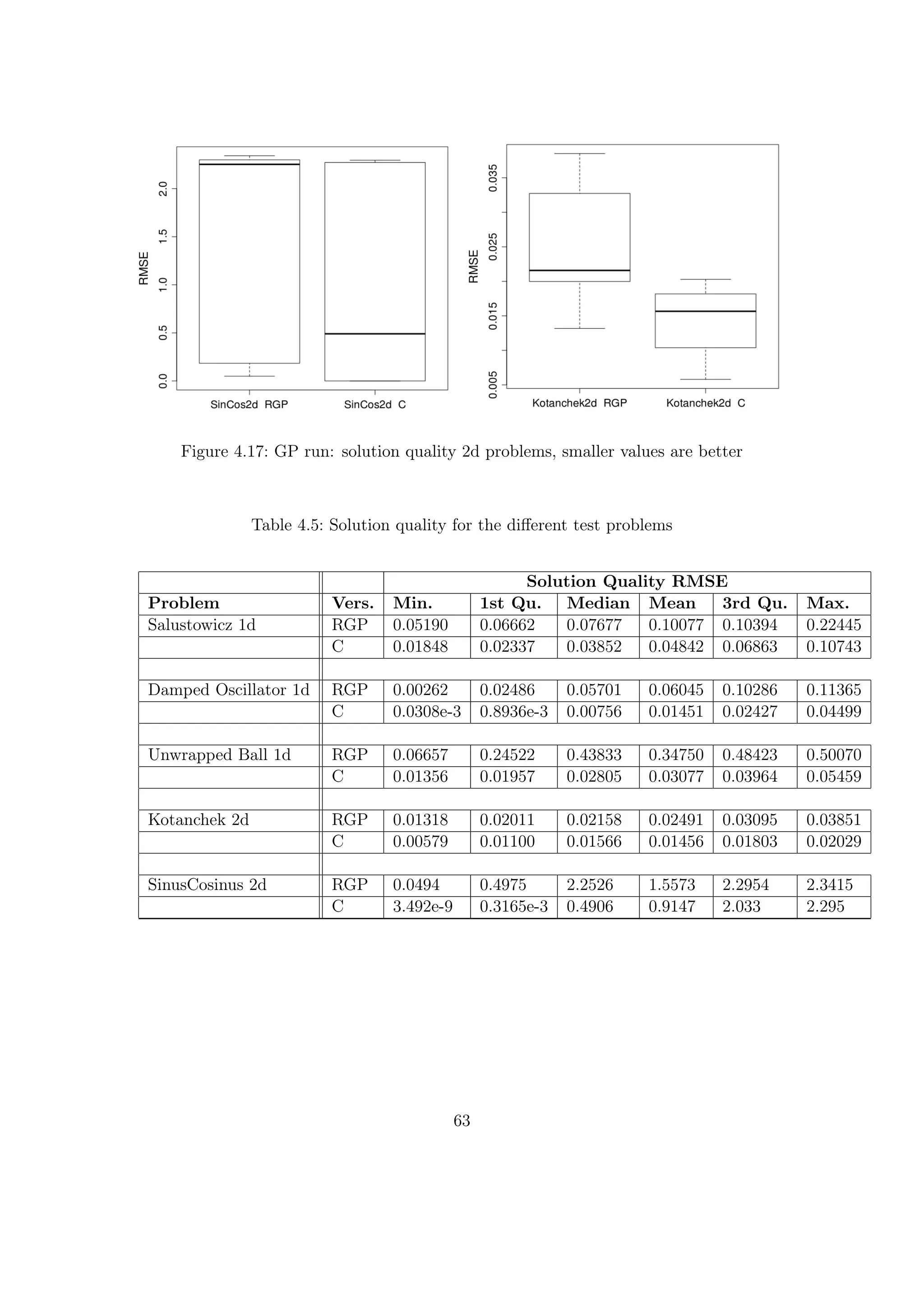
![Result Table
Table 4.4: Evolution steps for a time budget of 360 seconds
Evolution Steps
Problem Vers. Min. 1st Qu. Median Mean 3rd Qu. Max.
Salustowicz 1d RGP 3124 4320 5084 4731 5486 5566
C 433594 451225 487627 536267 542417 782853
Gain 95.91 113.35
Damped Oscillator 1d RGP 3008 3202 3589 3741 4126 5151
C 389479 417318 478049 487057 551984 610288
Gain 133.19 130.19
Unwrapped Ball 1d RGP 2181 3056 3202 3339 3423 4709
C 507292 613634 675082 724275 876777 993468
Gain 210.83 216.91
Kotanchek 2d RGP 4138 4970 6966 10932 14155 30098
C 22108 25202 29089 32335 34873 45262
Gain 4.18 2.96
SinusCosinus 2d RGP 2903 3464 3954 3979 4218 5702
C 23317 32472 36135 41630 42590 81847
Gain 9.14 10.46
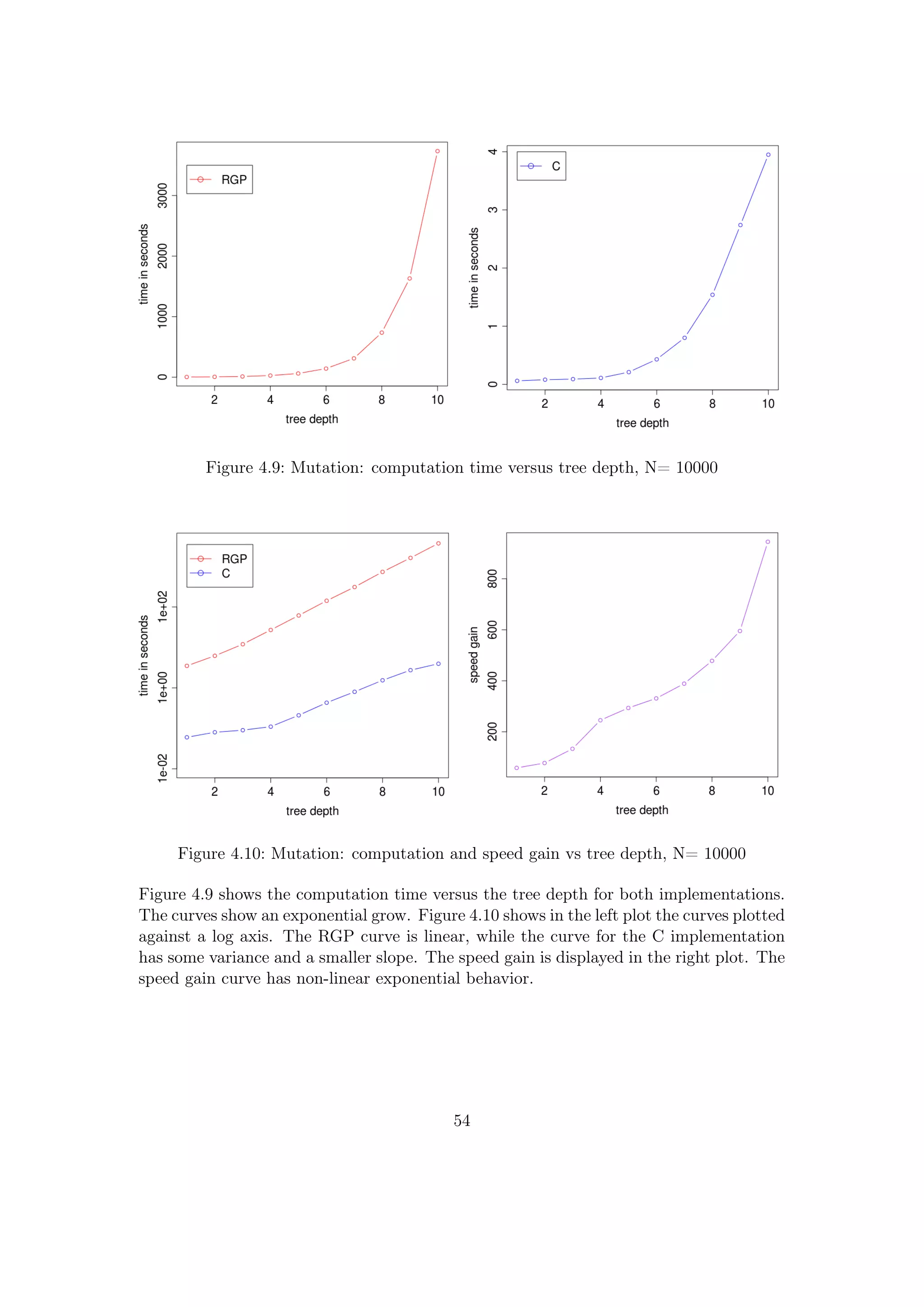
The results shown in the Figures 4.13 and 4.14 and display the behavior of both im-
plementations for the different functions. The Table 4.4 shows the different values in
comparison and the medium and mean speed gain for each function. RGP has an inter-
esting behavior, as it is faster for the 2d functions with the bigger sized input vectors.
The C implementation is very fast for the 1d problems, but gets much slower (factor
[10;20]) for the 2d problems.
Thus the speed gain is high for the one-dimensional test problems with small sized input
vectors with 64 samples points. For the two-dimensional problems with 2500 samples
points per variable, the speed gain gets much lower.
61](https://image.slidesharecdn.com/7917a8af-6d0a-4b34-9fa4-99117e0f65d0-160111142603/75/Thesis-67-2048.jpg)

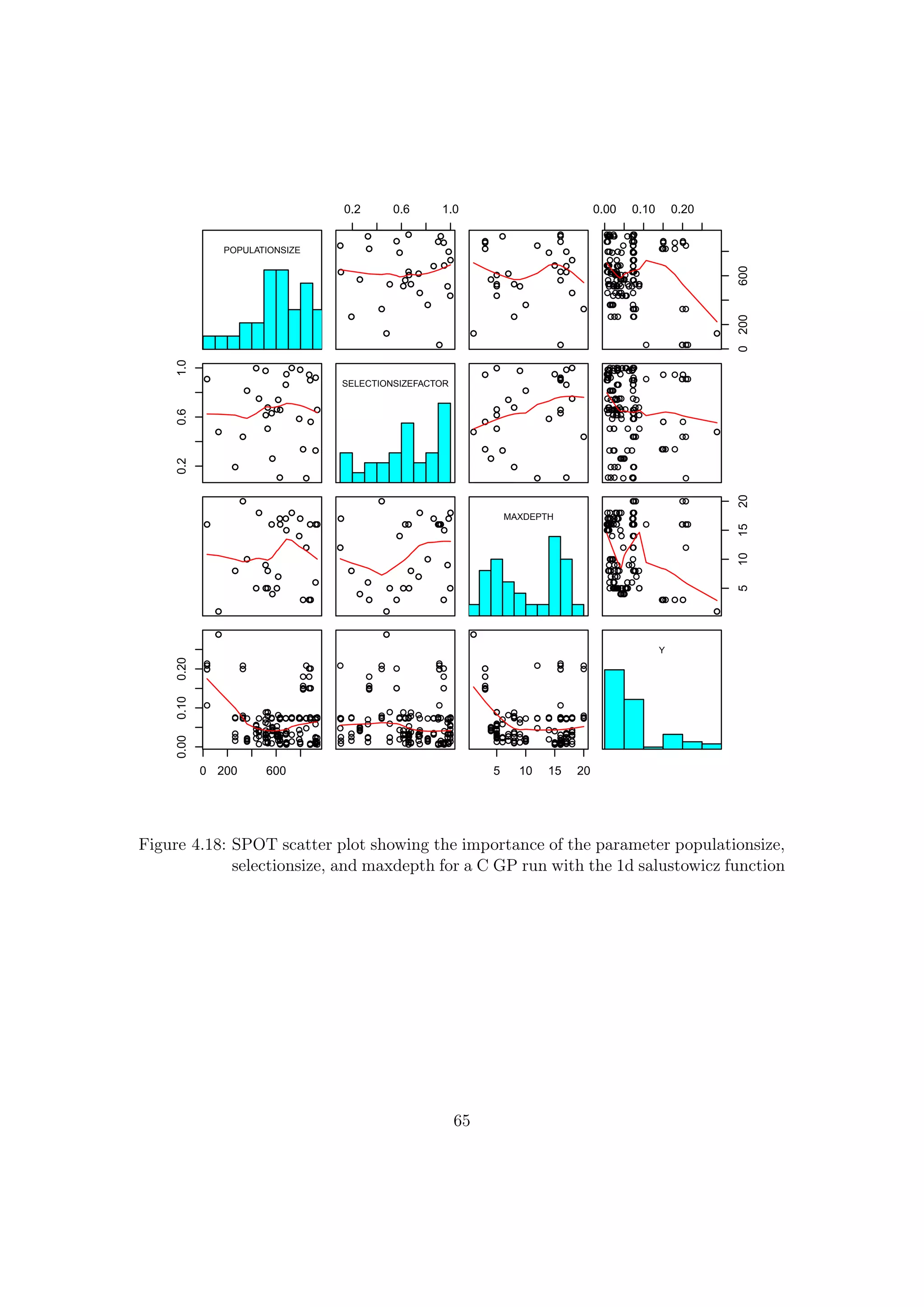
![4.3 SPOT Parameter Tuning
To improve the setup for the DataModler comparison, a sequential parameter optimiza-
tion(SPO) with SPOT [6, 5, 3] is performed. SPO is described as follows:
Sequential parameter optimization (SPO) is a heuristic that combines classical and mod-
ern statistical techniques to improve the performance of search algorithms. It includes a
broad variety of meta models, e.g., linear models, random forest, and Gaussian process
models (Kriging).[4]
SPO uses the available budget sequentially, explores the search space and builds one
or more meta-models. With the prediction of these meta-models new design points are
chosen and the meta-models are renewed. Ultimately it shows how the parameters be-
have in certain combinations.
In this case, SPO is used to tune the parameters populationsize, selectionsize and maxdepth
for a C GP run with the salustowicz function. Before the tuning, the search space has
to be defined. The used setup was:
• time budget: 360 seconds per independent run, 5 runs per point
• populationsize range: [20;1000]
• selectionsize factor range: [0.1;1], selectionsize = factor × populationsize
• maxdepth range: [1;20]
• global time budget: 24h
Figure 4.18 shows a scatter-plot of the results. The selectionssize has to be >200 to get
good results, for a value of 600 there is least variance. The selectionsize shows the least
variance for a factor of 0.7, while the maxdepth has to be >5 to get good results. For
maxdepth=10 is a good point with low variance. The results of this tuning will be used
in the comparison of the C implementation with DataModeler.
64](https://image.slidesharecdn.com/7917a8af-6d0a-4b34-9fa4-99117e0f65d0-160111142603/75/Thesis-70-2048.jpg)
![4.4 Comparison with DataModeler
In this comparison, the solution quality of the improved RGP system is measured against
DataModeler.[7, 15, 25] DataModeler is an commercial state-of-the-art GP system, the
developer describes it as follows:
DataModeler features state-of-the-art algorithms for symbolic regression via genetic pro-
gramming. Among the many benefits are rapid development of transparent human inter-
pretable models and identification of driving variables and variable combinations. Cor-
related variables are naturally handled and effective models may be built from large and
ill-conditioned data sets. Models may also have trust metrics to allow their use in dy-
namic data environments.[7]
This test covers two test problems, for each training and test sets were created. For the
one-dimensional problem, an interpolated test set was used, while an extrapolated test
set was used for the two-dimensional problem.
4.4.1 Comparison Setup
The detailed setup for this comparison was:
• DataModeler and C implementation
– function set: +, -, *, /, sin, cos, exp, log, sqrt
– 360 seconds budget per independent evolution run
– 32 independent runs per problem
• DataModeler
– default parameters, population size: 300
• C implementation
– population size N: 600, selection size: 420, maximal depth: 10
– maximal number of leaves: 250, maximal number of nodes= 250;
– constant probability: 0.3, constant scaling factor: 5, subtree probability: 0.7
66](https://image.slidesharecdn.com/7917a8af-6d0a-4b34-9fa4-99117e0f65d0-160111142603/75/Thesis-72-2048.jpg)
![4.4.2 test problems
Figure 4.19: Two-dimensonal salustowicz function
The problems for this comparison were the one- dimensional salustowicz function ( Sec-
tion 4.2.1 ) and the two-dimensional salustowicz function, displayed in Figure 4.19.
Salustowicz 2d:
f(x) = exp(−x1) × x3
1 × (x2 − 5) sin(x1) × cos(x1) × (sin(x1)2 × cos(x1) − 1)
salustowicz 1d interpolation problem
training set: range x: [0;12] 64 samples
test set range x:[0;12] 256 samples
salustowicz 2d extrapolation problem
training set: range x1, x2: [0;12] 32 samples, input vector: 32 × 32 = 1024
test set: range x1, x2: [-1,13] 40 samples, input vector: 40 × 40 = 1600
67](https://image.slidesharecdn.com/7917a8af-6d0a-4b34-9fa4-99117e0f65d0-160111142603/75/Thesis-73-2048.jpg)

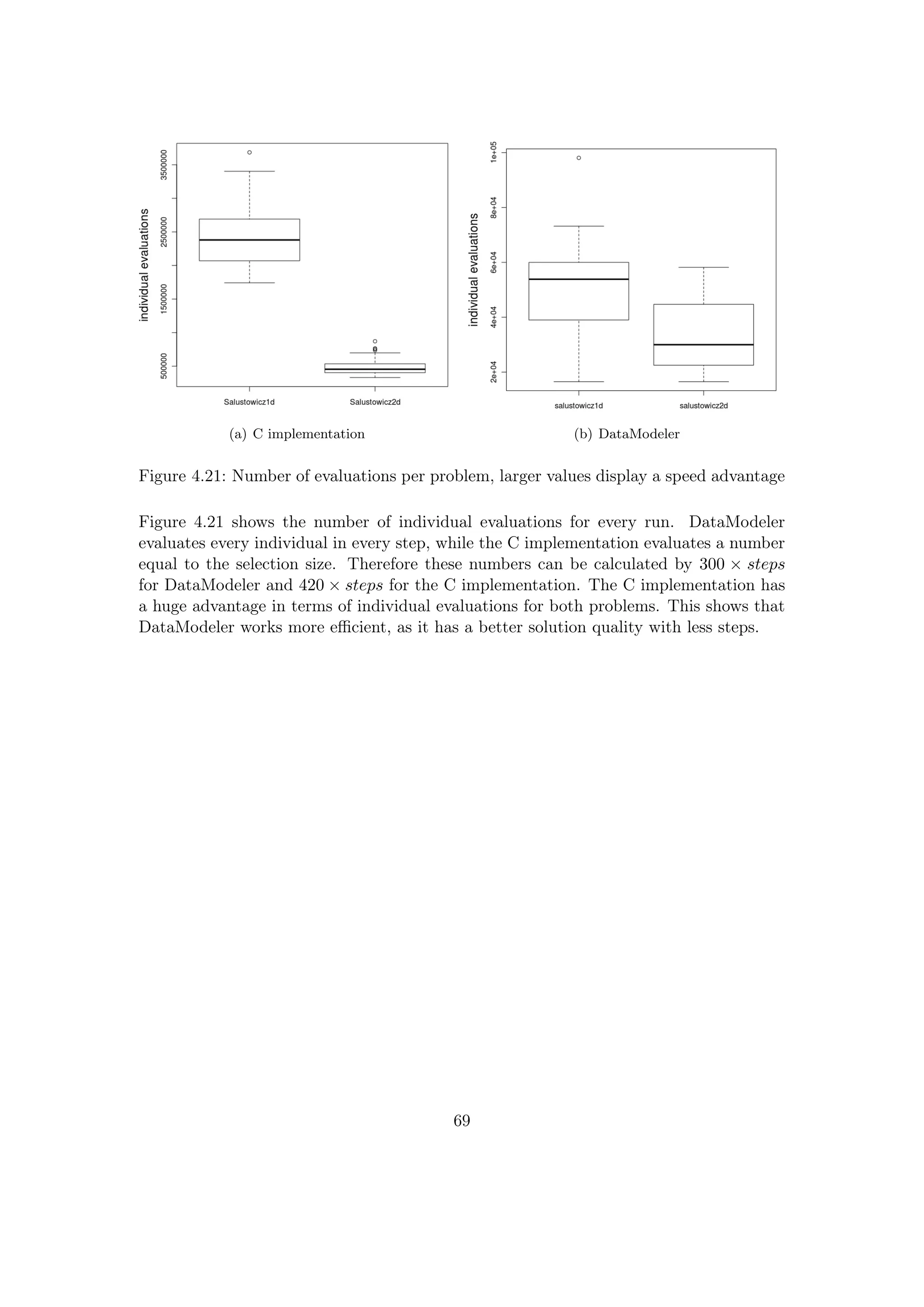
![5 Discussion
This chapter deals with possible explanations for the results. First the prior expecta-
tions are listed in comparison to the achieved results, then the experiments are discussed.
Finally, the results of the SPOT tuning and the comparison with DataModeler are re-
viewed.
5.1 Prior Expectations versus Achieved Results
Initially there were some expectations regarding the achievable speed gain trough imple-
menting the RGP functions in C. The expectations for the speed gain were based on the
following assumptions:
• there is a speed difference between compiled and interpreted languages
• loops and recursions are faster in C
• there is a speed gain due specialized and thus smaller functions
The Table 5.1 shows a comparison of the expectations and the results. Here td is the
tree depth, while iv is the input vector.
Table 5.1: Expectations and Results
Function Note Expected Gain Achieved Gain
Initialization [10;50]
Min. small td 350
Max. large td 650
Evaluation [50;100]
Min. small td and large iv 0.99
Max. large td and small iv 24.5
Mutation [10;50]
Min. small td 58
Max. large td 945
GP run [50;100]
Min. 2d large iv 3
Max. 1d small iv 216
70](https://image.slidesharecdn.com/7917a8af-6d0a-4b34-9fa4-99117e0f65d0-160111142603/75/Thesis-76-2048.jpg)
![5.2 Call-by-Value versus Call-by-Reference
To understand the results it is essential to take a deeper look into the R language and
how it handles values and objects. The R language uses solely the call-by-value method
for functions. [21] This means that in R on every function call all actual parameters are
copied, involving memory allocation with possible garbage collection and full traversal of
the of the data structures copied.1 The initialization and mutation heavily use recursive
functions to build or analyze the individual trees. This results in a huge amount of copy
operations for large tree depths.
For example, in a delete-subtree mutation (Section 2.3.5) the individual tree has to be
completely analyzed to measure the number of suitable subtrees. If a node is found, the
function is called recursively with the left and right subtree. For each recursive call the
subtrees of the current node and the all actual parameters have to be copied. This is
done for each node in the tree. For a full tree with the depth 7 and only functions of
arity two, the number of nodes is 127 (Section 4.1.1), resulting in the same number of
copy operations. This has a large negative impact on the computation performance, e.g,
a large full tree with depth 10 has 1023 nodes. The copied subtrees are in this case also
larger, therefore they require more memory and the copy operations are also slower.
C supports the call-by-reference method. In this method the actual parameters are
not copied, instead, a memory pointer to the data is used in the function. It is also
possible to directly modify this data, which is heavily used in the mutation functions.
The R structures are also linked pointer lists and can be passed very quickly by the
provided C macros (see Section 3.3.1). This ultimately leads to the high speed gain for
the initialization and mutation function, in which the trees are build or analyzed.
5.3 Optimized Evaluation
Initially the assumption was made, that the R eval() is kind of slow due the large
supported function set. But the results have shown that the R eval() is highly optimized
to support large input vectors and the mathematical operations are performed quite fast.
The speed gain trough the faster pointer arithmetic in C (Section 5.2) can be seen for
small input vectors and large tree sizes. In this cases, the speed gain is significant.
But as soon as the input vectors get large, the computation time is dominated by the
mathematical operations. This results in a much smaller speed gain around or even
below one (for very small trees). An explanation is that the R eval() uses a algorithm
which is highly optimized for large input vectors and even outperforms the specialized
C evaluator in terms of computation speed for vectorized mathematical operations. The
overall performance of the C evaluator is due to the faster pointer arithmetic still better
for the analyzed cases, with exception to very small trees (nodes <= 4).
1
to be exact, actual parameters are only copied when their values are referred to in the body the
function called
71](https://image.slidesharecdn.com/7917a8af-6d0a-4b34-9fa4-99117e0f65d0-160111142603/75/Thesis-77-2048.jpg)
![6 Conclusion
This thesis started with the description and performance analysis of RGP, a GP system
implemented in the high level programming language R. Afterwards, a concept to accel-
erate this system was designed and introduced. This concept lead to certain implemen-
tation tasks: First, the speed critical functions had to be implemented in C. Second, the
GP main loop had to be implemented in C. Third, other methods for improving the over-
all performance of the system had to be explored. A complete GP run was implemented
in C, thus the first and second objective were successfully achieved. The implementation
also contains some novel ideas, like a new additional uniform depth-regarding crossover
and new additional variation operators. These operators can improve the performance
of the system on some test problems, therefore the third objective is also fulfilled.
The experiments conducted with the new C implementation have shown the achievable
speed gain to vary greatly. The main factors influencing the speed gain are the maxi-
mal depth of the individuals and the size of the input vectors for each variable. The C
implementation has a substantial speed advantage for the initialization and mutation op-
erations, particularly when individuals get large (>50 nodes). The evaluation operation
has a significant speed gain as long as input vectors stay relatively small (<100 values).
Larger input vectors lead to a reduced speed gain. These facts influence the effective
speed gain for the complete GP run. For small sized input vectors, the speed gain is in
the range of [100, 200], for larger input vectors (>2000 values), the speed gain is in the
range [1, 10]. This also affects the solution quality achievable by the C implementation
in evolution runs with a fixed time budget, since less evolution steps can be performed.
Although the DataModeler comparison has shown that the C implementation of RGP
performs competitive for small dimensions at the first glance, it should be noted that
these results were obtained with a SPOT tuned version whereas DataModeler was not
tuned at all.
The experiments have therefore shown, that a C implementation has a huge impact on
the performance in cases where the individual trees have to be analyzed. This applies
especially for the uniform mutation and crossover operators where the complete indi-
vidual trees have to be analyzed multiple times. The R evaluation is already fast and
highly optimized for mathematical operations with large vector sizes(1.e+6), so that no
significant gain could be achieved by the C implementation for this cases. For even larger
input vectors, the R eval() might even be faster. This fact could be taken care of by
defining a vector size limit(>1.e+6) at which a fall back to the R eval() will be used.
This switching point would be easy implementable, since the R eval() can be called
from C.
73](https://image.slidesharecdn.com/7917a8af-6d0a-4b34-9fa4-99117e0f65d0-160111142603/75/Thesis-79-2048.jpg)


![Bibliography
[1] R. Adams. Take command: The m4 macro package. Linux Journal, 2002(96):6,
2002.
[2] Th. Bartz-Beielstein, O. Flasch, P. Koch, and W. Konen. SPOT: A toolbox for in-
teractive and automatic tuning in the R environment. In F. Hoffmann and E. Hüller-
meier, editors, Proceedings 20. Workshop Computational Intelligence, pages 264–273.
Universitätsverlag Karlsruhe, 2010.
[3] Thomas Bartz-Beielstein. Experimental Research in Evolutionary Computation—
The New Experimentalism. Natural Computing Series. Springer, Berlin, Heidelberg,
New York, 2006.
[4] Thomas Bartz-Beielstein and Matina Friese. Sequential parameter optimization and
optimal computational budget allocation for noisy optimization problems. CIOP
Technical Report 02/11, Research Center CIOP (Computational Intelligence, Op-
timization and Data Mining), Cologne University of Applied Science, Faculty of
Computer Science and Engineering Science, January 2011.
[5] Thomas Bartz-Beielstein, Christian Lasarczyk, and Mike Preuß. Sequential param-
eter optimization. In B. McKay et al., editors, Proceedings 2005 Congress on Evo-
lutionary Computation (CEC’05), Edinburgh, Scotland, volume 1, pages 773–780,
Piscataway NJ, 2005. IEEE Press.
[6] Thomas Bartz-Beielstein, Konstantinos E. Parsopoulos, and Michael N. Vrahatis.
Design and analysis of optimization algorithms using computational statistics. Ap-
plied Numerical Analysis and Computational Mathematics (ANACM), 1(2):413–433,
2004.
[7] Evolved Analytics LLC. DataModeler 8.0. Evolved Analytics LLC, 2010.
[8] O. Flasch, T. Bartz-Beielstein, P. Koch, and W. Konen. Clustering Based Niching
for Genetic Programming in the R Environment. In Proceedings: 20. Workshop
Computational Intelligence; Dortmund, 1.-3. Dezember 2010, page 33. KIT Scientific
Publishing, 2010.
[9] O. Flasch, Th. Bartz-Beielstein, A. Davtyan, P. Koch, W. Konen, T.D. Oyetoyan,
and M. Tamutan. Comparing SPO-tuned GP and NARX prediction models for
stormwater tank fill level prediction. In Gary et al. Fogel, editor, Proc. IEEE
Congress Evolutionary Computation (CEC), pages 1579–1586, 2010.
77](https://image.slidesharecdn.com/7917a8af-6d0a-4b34-9fa4-99117e0f65d0-160111142603/75/Thesis-83-2048.jpg)
![[10] O. Flasch, Th. Bartz-Beielstein, P. Koch, and W. Konen. Diversity Preservation
Methods for Genetic Programming in the R Environment. In F. Hoffmann and
E. Hüllermeier, editors, Proceedings 20. Workshop Computational Intelligence. Uni-
versitätsverlag Karlsruhe, 2010. in print.
[11] Oliver Flasch, Thomas Bartz-Beielstein, Patrick Koch, and Wolfgang Konen. Ge-
netic Programming Applied to Predictive Control in Environmental Engineering. In
Frank Hoffmann and Eyke Hüllermeier, editors, Proceedings 19. Workshop Compu-
tational Intelligence, pages 101–113, Karlsruhe, 2009. KIT Scientific Publishing.
[12] Oliver Flasch, Olaf Mersmann, and Thomas Bartz-Beielstein. RGP: An open source
genetic programming system for the R environment. In Martin Pelikan and Jürgen
Branke, editors, Genetic and Evolutionary Computation Conference, GECCO 2010,
Proceedings, Portland, Oregon, pages 2071–2072. ACM, 2010.
[13] Thomas Girke. Programming in R. UC Riverside, 2008.
[14] S. Højsgaard. Calling C functions from R using .C and .Call. Department of Molec-
ular Biology and Genetics, Aarhus University, January 2010.
[15] Mark Kotanchek, Guido Smits, and Ekaterina Vladislavleva. Pursuing the pareto
paradigm tournaments, algorithm variations & ordinal optimization. In Genetic
Programming Theory and Practice IV, volume 5 of Genetic and Evolutionary Com-
putation, chapter 12, pages 167–186. Springer, 11-13 May 2006.
[16] U. Ligges and J. Fox. R help desk: How can i avoid this loop or make it faster. R
News, 8(1):46–50, 2008.
[17] L. Ljung. Perspectives on system identification. Annual Reviews in Control, 34(1):1–
12, 2010.
[18] Sean Luke. Essentials of Metaheuristics. 2009. available at
http://cs.gmu.edu/∼sean/book/metaheuristics/.
[19] D.J. Montana. Strongly typed genetic programming. Evolutionary computation,
3(2):199–230, 1995.
[20] Riccardo Poli, William B. Langdon, and Nicholas Freitag McPhee. A field guide
to genetic programming. Published via http://lulu.com and freely available at
http://www.gp-field-guide.org.uk, 2008. (With contributions by J. R. Koza).
[21] R Development Core Team. An Introduction to R. R Foundation for Statistical
Computing, Vienna, Austria, 2011. ISBN 3-900051-11-9.
[22] R Development Core Team. R: A Language and Environment for Statistical Com-
puting. R Foundation for Statistical Computing, Vienna, Austria, 2011. ISBN
3-900051-07-0.
78](https://image.slidesharecdn.com/7917a8af-6d0a-4b34-9fa4-99117e0f65d0-160111142603/75/Thesis-84-2048.jpg)
![[23] R Development Core Team. R Internals. R Foundation for Statistical Computing,
Vienna, Austria, 2011. ISBN 3-900051-11-9.
[24] Luke Tierney, A. J. Rossini, Na Li, and H. Sevcikova. snow: Simple Network of
Workstations, 2009. R package version 0.3-3.
[25] Ekaterina Vladislavleva. Model-based Problem Solving through Symbolic Regression
via Pareto Genetic Programming. PhD thesis, Tilburg University, Tilburg, the
Netherlands, August 2008.
79](https://image.slidesharecdn.com/7917a8af-6d0a-4b34-9fa4-99117e0f65d0-160111142603/75/Thesis-85-2048.jpg)