This document discusses Bayesian analysis of the Weibull distribution using different priors in S-Plus software. It proposes a new lifetime distribution that is an extension of the Weibull distribution and derives the Weibull distribution as a special case of the proposed model. It describes the likelihood and posterior distributions for the Weibull parameters under different prior distributions and discusses Bayesian estimation methods and a simulation study to compare the mean square error of the estimators.

1. www.ijemr.net ISSN (ONLINE): 2250-0758, ISSN (PRINT): 2394-6962
64 Copyright © 2018. IJEMR. All Rights Reserved.
Volume-8, Issue-5, October 2018
International Journal of Engineering and Management Research
Page Number: 64-69
DOI: doi.org/10.31033/ijemr.8.5.03
On Extension of Weibull Distribution with Bayesian Analysis using S-Plus
Software
Bilal Ahmad Bhat
Associate Professor (Statistics), Division of Social Science, Faculty of Fisheries, SKUAST-Kashmir,Rangil Ganderbal, J&K,
INDIA
Corresponding Author: bhat_bilal@rediffmail.com
ABSTRACT
We introduce a new lifetime distribution which is an
extension of Weibull distribution and yields a number of well-
known distributions as a special case. The Bayesian analysis
using different priors is discussed using different priors with
the help of S-Plus software as nowadays great attention has
been given to Bayesian approach.
Keywords-- Weibull distribution, Bayesian method, Prior,
Probability density function, Statistical model
I. INTRODUCTION
One of the most remarkable application of
probability theory is to depict the real life phenomenon
through probability model or distribution. Statistical
models describe a phenomenon in the form of
mathematical equations. In the literature (Hogg & Crag
(1970), Johnson & Kotz (1970), Lawless (1982) etc.) we
come across different types of models e.g., Linear models,
Non-linear models, Generalized linear models,
Generalized addition models, Analysis of variance models,
Stochastic models, Empirical models, Simulation models,
Diagnostic models, Operation research models, Catalytic
models, Deterministic models, etc. Out of large number of
methods and tools developed so far for analyzing data (on
the life sciences etc.), the statistical models are the latest
innovations.
Weibull distribution was originally derived in
1928 by Professor R.A.Fisher and L.H.C. Tippet and
became known to researchers as the Fisher-Tippet Type III
distribution. In 1939, Waloddi Weibull developed this
distribution for analysis of breaking-strength data and he
also published several other papers on the wide
applicability of the distribution. The use of Weibull
distribution in reliability and quality control is well known.
The distribution is also useful in cases where the
conditions of strict randomness of exponential distribution
are not satisfied. It is some times used as a tolerance
distribution in the analysis of quantal response data. The
main justification for consideration of the Weibull
distribution is that it has been shown experimentally to
provide a good fit for many different types of
characteristics since Waloddi Weibull derived it in an
analysis of breaking strengths (Sinha (1986)). It is perhaps
the most popular parametric family of distributions, being
used as a failure model
In this paper, we propose a model which is an
extension of the model proposed by Bilal (2011) and
includes weibull distribution as a special case. Finally, we
discuss Bayesian method of estimation in case of Weibull
distribution. It is interesting to note that researchers are
trying to find out which estimation method is preferable
for the parameter estimation of a particular probability
distribution in order to get reliable estimates of the
parameters.
The most popular and easiest methods of utilizing
data from a random sample to estimate the parameters of
the Weibull distribution have been the log-log graphical
plot, the Weibull graphical plot, least square estimates,
moment estimates, maximum likelihood estimates and the
several more complicated methods proposed by
statisticians in technical journals.
II. BAYESIAN APPROACH
Bayesian Statistics is an approach to statistics which
formally seeks use of prior information with the data, and
Bayes Theorem provides the formal basis for making use
of both sources of information in a formal manner. Bayes
Theorem states that

2. www.ijemr.net ISSN (ONLINE): 2250-0758, ISSN (PRINT): 2394-6962
65 Copyright © 2018. IJEMR. All Rights Reserved.
Posterior  likelihood x prior
The prior is the probability of the parameter and represents
what was thought before seeing the data. The likelihood is
the probability of the data given the parameter and
represents the data now available.
The posterior represents what is thought given both prior
information and the data just seen. It relates the conditional
density of a parameter (posterior probability) with its
unconditional density (prior, since depends on information
present before the experiment).
or equivalently Bayes’ Theorem for a given parameter
 is given by
p ( data) = p (data ) p () / p (data)
1/p (data) is basically a normalizing constant
In spite of problems, Bayesian methods are very
popular with statisticians, even those who don’t accept
subjective Bayesian principles. Empirical Bayesian
statisticians use conjugate priors (priors that lead to simple
posteriors), uninformative priors (priors like the uniform
distribution), and improper priors (priors like the uniform
distribution on an infinite interval), to arrive at estimates
like those of classical sampling theory.
III. PROPOSED MODEL
Let g(x) be a continuous monotonic increasing
function in (k,  ) such that g(  )=  and g(k)=0 where k
is any positive real number, then the function
     ;)(exp)(')()(),,,,;( )()(1 xgxg
exgxgexgxggxf 
  
(1.1)
where α, θ, β and λ are non-negative, with θ
being shape parameter and α, and β being scale
parameters and λ acceleration parameter. The function
(1.1) can exhibit different behaviour depending on g(x)
and the values of the parameters chosen.
IV. DERIVATION OF WEIBULL
DISTRIBUTION
In fact, a number of new of new and some well-
known distributions follow the model(1.1) for a suitable
choice of the function g(x) and the parameters of the
proposed model. Here we mention Weibull model
Remark 1.1. Taking g(x)=x so that gˊ(x)=1 and
β=0 in (1.1), we have
f(x / ), =  
 xx 
exp1
; x, 0, 
= 0 otherwise
Which is the pdf of well-known two parameter
Weibull distribution with parameters α >0 and ɵ>0.
Similarly as above, many more distributions can
be shown as a particular case of the proposed statistical
model (1.1) for a suitable choice of the generating function
g(x) and the parameters.
V. METHODS OF ESTIMATION OF
WEIBULL MODEL
The probability density function of Weibull
model is given by
f(x / ), = 







 
 x
x exp1
; x, 0, 
= 0 otherwise (1.1.1)
If x1, x2, …, xn be iid observations from weibull
model, then the likelihood function is given by

3. www.ijemr.net ISSN (ONLINE): 2250-0758, ISSN (PRINT): 2394-6962
66 Copyright © 2018. IJEMR. All Rights Reserved.
L(x,α,θ)=  ),,( xf
= 







 n
n
in
n
x 





exp
1
The maximum likelihood estimator is given by
 

n
xi
(1.1.2)
Suppose shape parameters α be known and let
g(θ) 0,1,,
)/exp(


 


ca
a
c
(1.1.3)
be the prior distribution of θ. Then its posterior is










 

 cn
i ax
Kx




exp
)/( (1.1.4)
where
  1
0
1 )1(
exp

















 

 cn
i
cn
i
ax
cn
d
ax
K





Bays Estimator of θ is given by
1



cn
axi


In case of Jeffrey’s invaria nt prior, the prior
distribution of (θ, α) is g(θ) h(α) where
.,1)(0,1)( aaahandcg c  

 Wit
h these priors, the posterior distribution of (θ,α) is given by










 







 i
cn
n
xK
x exp)/,( 1
(1.1.5)
where






d
x
cnddxKandx cnn
i
i
nn
i
i 

 











0
1
1
1
0 0
1
1
)1()/,(

4. www.ijemr.net ISSN (ONLINE): 2250-0758, ISSN (PRINT): 2394-6962
67 Copyright © 2018. IJEMR. All Rights Reserved.
The Marginal posterior of α is given by






















 








0
1
1
1
1
1
1
)/(
d
x
x
x
cnn
i
i
n
cnn
i
i
n
(1.1.6)
Under square error loss function ,)ˆ()ˆ(   cl the risk function is given by





 





 












 

 
c
n
c
n
xc
c
n
xc
cR
n
i
i
n
i
i
211
ˆ2
ˆ)ˆ(
2
112

 (1.1.7)
and the Bays Estimator as





 


c
n
x
n
i
i
1
ˆ 1
2
Now under the loss function   )ˆ(l )ˆ(   , we obtain the Bays Estimators as















c
n
x
n
i
i
2
3
ˆ 1
3
VI. SIMULATION STUDY
In the simulation study, we have chosen n=35, 75,
100 to represent small, moderate and large sample size,
several values of the parameters α = 0.5, 1, 1.5, 2 with four
values of constants. The number of replication used was
R=1000. The simulation program was written by using S-
Plus/R software. After the parameter was estimated, mean
square error (MSE) and mean percentage error MPE were
calculated. We have
 
R
MPEand
R
MSE ii
 




1000
1
1000
1
ˆ
)ˆ(
ˆ
)ˆ(





VIII. RESULTS
Table 1 : Estimators with respect to MSE
Size of Sample   1

2

3

35 0.5 0.4
0.8
0.2001
0.2001
0.1349
0.1320
0.2120
0.2120

5. www.ijemr.net ISSN (ONLINE): 2250-0758, ISSN (PRINT): 2394-6962
68 Copyright © 2018. IJEMR. All Rights Reserved.
1 0.4
0.8
0.2221
0.2221
0.2089
0.2088
0.2287
0.2288
1.5 0.4
0.8
0.2343
0.2342
0.2322
0.2324
0.2335
0.2336
75 0.5 0.4
0.8
0.1248
0.1249
0.1213
0.1215
0.1289
0.1286
1 0.4
0.8
0.1231
0.1236
0.1201
0.1203
0.1223
0.1228
1.5 0.4
0.8
0.1266
0.1281
0.1249
0.1261
0.1304
0.1329
100 0.5 0.4
0.8
0.0887
0.0888
0.0886
0.0886
0.0939
0.0938
1 0.4
0.8
0.0886
0.0887
0.0858
0.0858
0.0874
0.0873
1.5 0.4
0.8
0.0886
0.0887
0.0854
0.0868
0.0888
0.0889
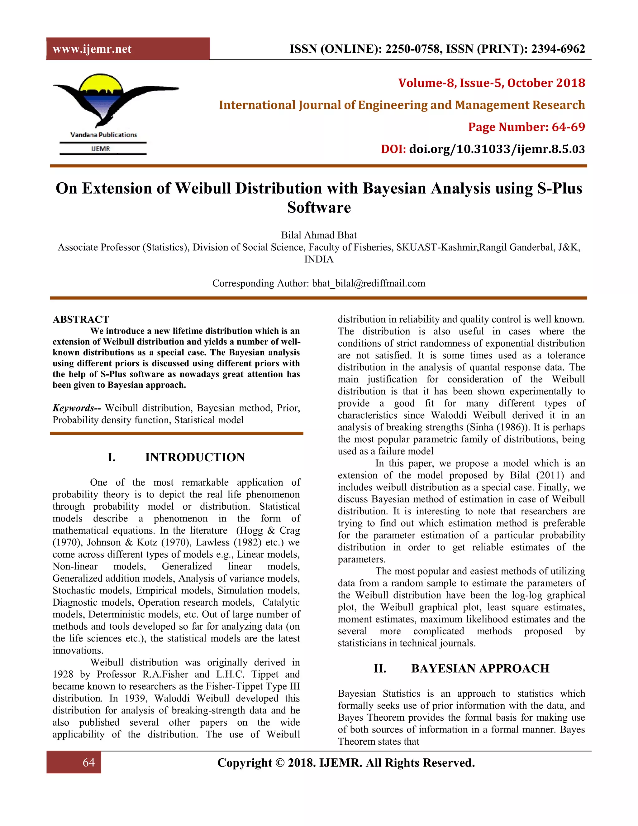
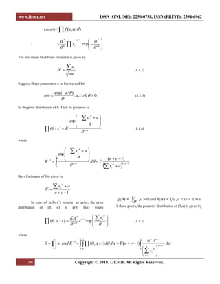
Table 2 : Estimators with respect to MPE
Size of Sample   1

2

3

35 0.5 0.4
0.8
0.0201
0.0203
0.0134
0.0131
0.0213
0.0212
1 0.4
0.8
0.0223
0.0224
0.0202
0.0203
0.0223
0.0224
1.5 0.4
0.8
0.0232
0.0233
0.0232
0.0232
0.0239
0.0241
75 0.5 0.4
0.8
0.0123
0.0124
0.0121
0.0122
0.0128
0.0141
1 0.4
0.8
0.0127
0.0129
0.0123
0.0122
0.0149
0.0148
1.5 0.4
0.8
0.0123
0.0124
0.0123
0.0123
0.0132
0.0133
100 0.5 0.4
0.8
0.0083
0.0082
0.0074
0.0073
0.0094
0.0093
1 0.4
0.8
0.0063
0.0064
0.0052
0.0053
0.0073
0.0072
1.5 0.4
0.8
0.0072
0.0073
0.0054
0.0053
0.0064
0.0063
VIII. CONCLUSION
The results obtained from the simulation study
presented in Table 1 and Table 2 reveals that Bayes
estimator with general Jeffery prior information, is the
best estimator when compared to standard Bayes and
Maximum likelihood estimator. The estimator with
smallest MSE is considered as best and with largest MSE
it is considered as worst. It is concluded that MSE and
MPE of Bayes estimators decrease with an increase of
sample size.
REFERENCES
[1] Bhat Bilal A. & A. B.Khan. (2011). A generalization
of gamma distribution. Adv. Res., 3(1), 90-91.
[2] Bhat Bilal A., T. A. Raja, M.S.Pukhta, & R.K.
Agnihotri. (2009). On a class of continuous type
probability distributions with application. International

6. www.ijemr.net ISSN (ONLINE): 2250-0758, ISSN (PRINT): 2394-6962
69 Copyright © 2018. IJEMR. All Rights Reserved.
Journal of Agricultural and Statistical Sciences, 6(1), 147-
156.
[3] Bhat Bilal A., A. Shafat, Raja T.A., & Parimoo R.
(2006). On a Class of Statistical Models and their
application in Agriculture. International Journal of
Agricultural and Statistical Sciences, 2(2), 265-274.
[4] Bhat Bilal A. Hassan, & S.A. Mir. (2003). a quick
method of obtaining weibull distribution and its bayesian
estimation. SKUAST Journal of Research, 2(2), 178-183.
[5] Hogg, R.V. & Craig, A.T. (1970). Introduction to
mathematical statistics. (4th
ed.). New York: Macmillan.
[6] Johnson, N.L. & Kotz, S. (1970). Continuous
univariate distributions, 1 and 2, Houghton Mifflin
Company, Bostan.
[7] Lawless, J.F. (1982). Statistical models and methods
for life-time data. New York: Wiley.
[8] McCullagh, P. & Nelder , J.A. (1988). Generalized
linear models. New York: Chapman and Hall.
[9] Sinha, S.K. (1986). Reliability and life testing. Wiley
Eastern Limited.
[10] S.P.Ahmad & Bilal Ahmad Bhat. (2010). Posterior
estimates of two parameter exponential distribution using
S-PLUS software. Journal of Reliability and Statistical
Studies, 3(2), 27-34.
[11] Venables, W.N. & Ripley, B.D. (2000). S
Programming. New York: Springer Verlag.