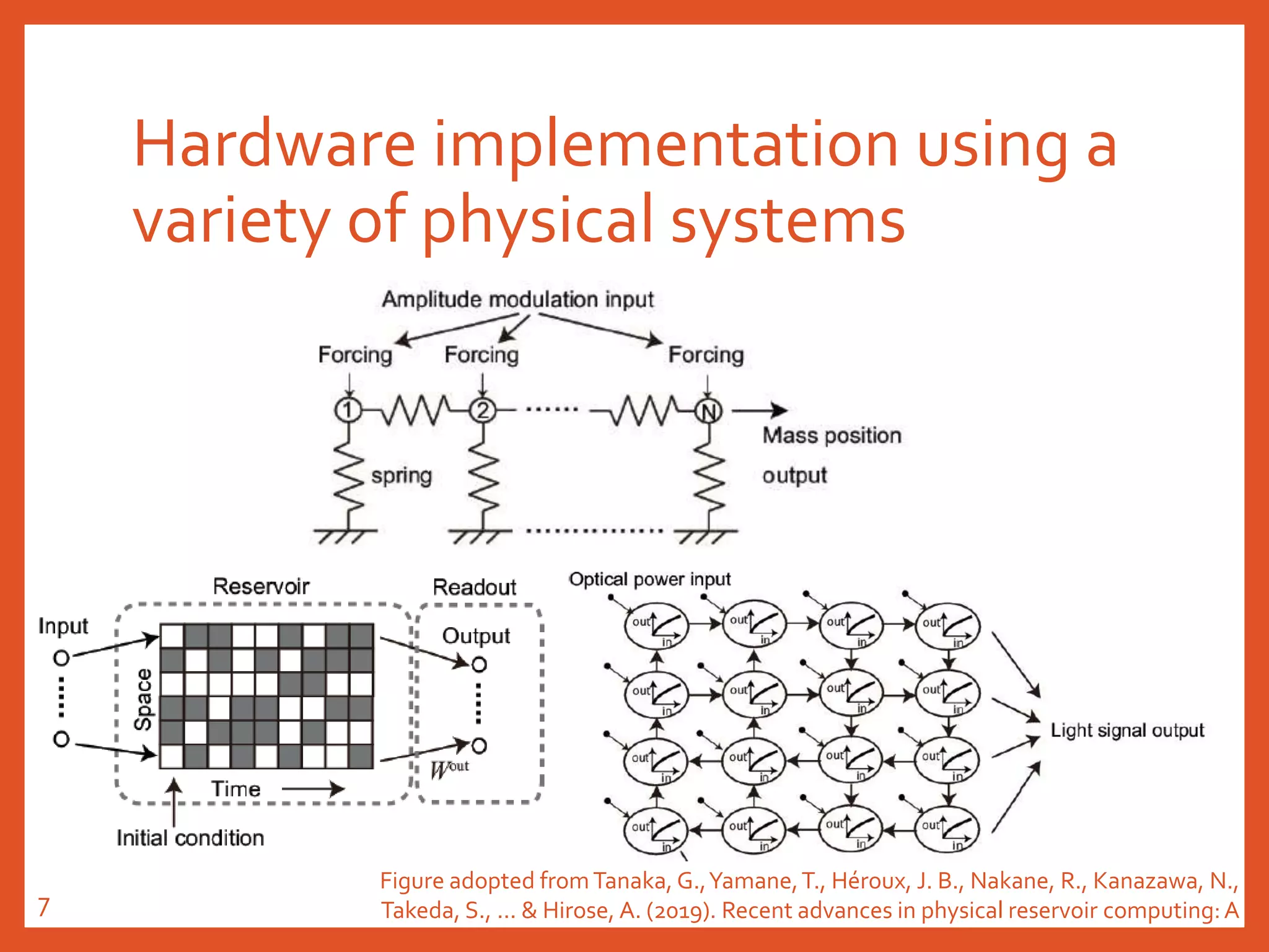
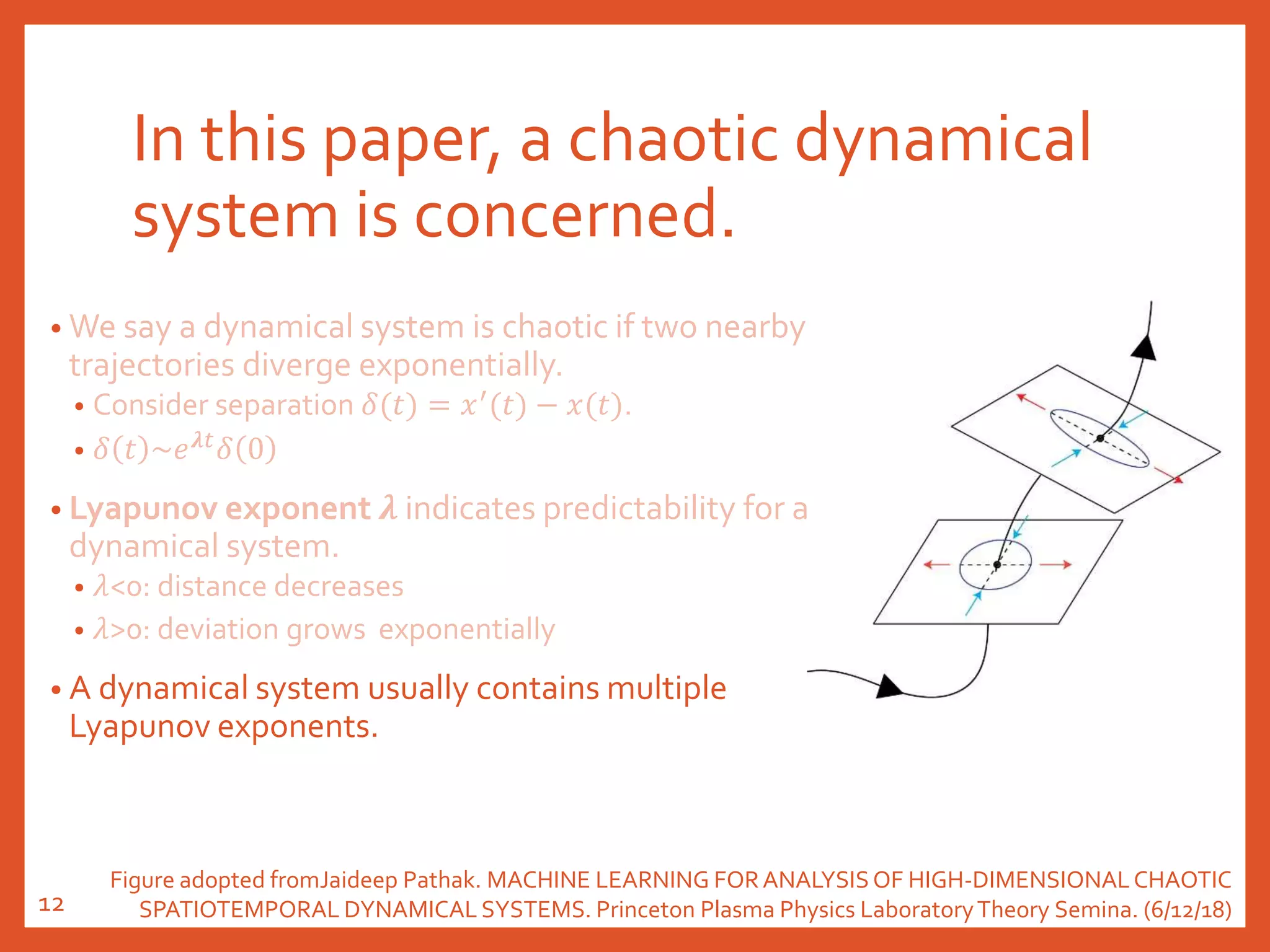
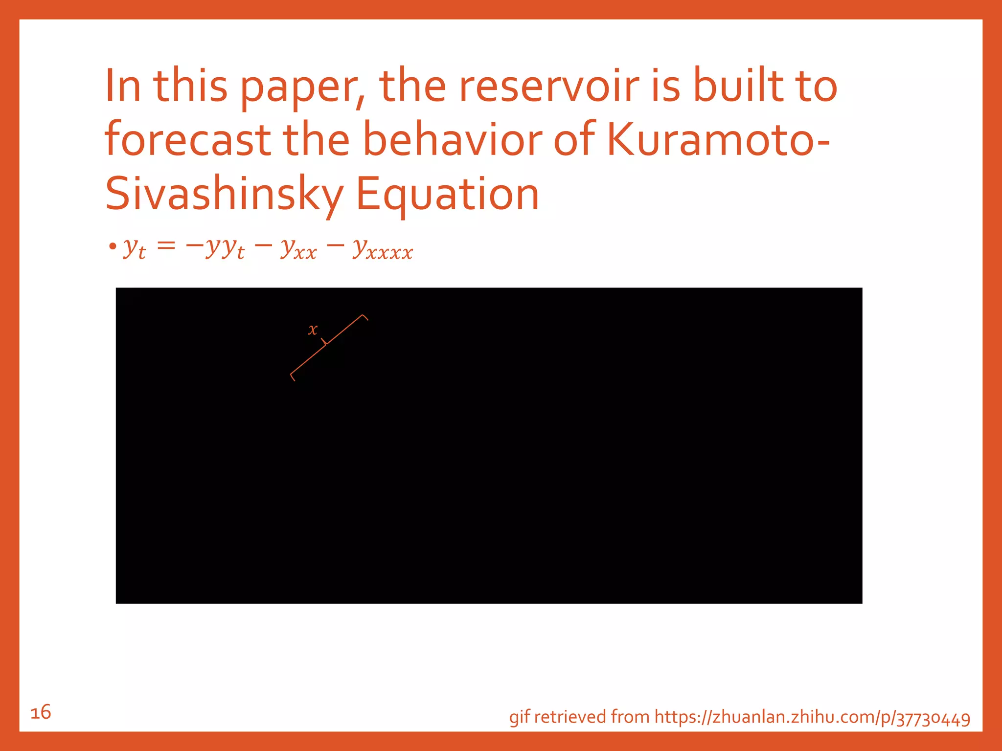
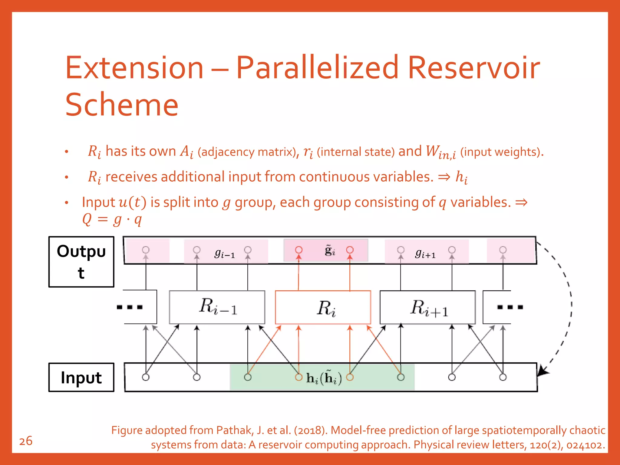
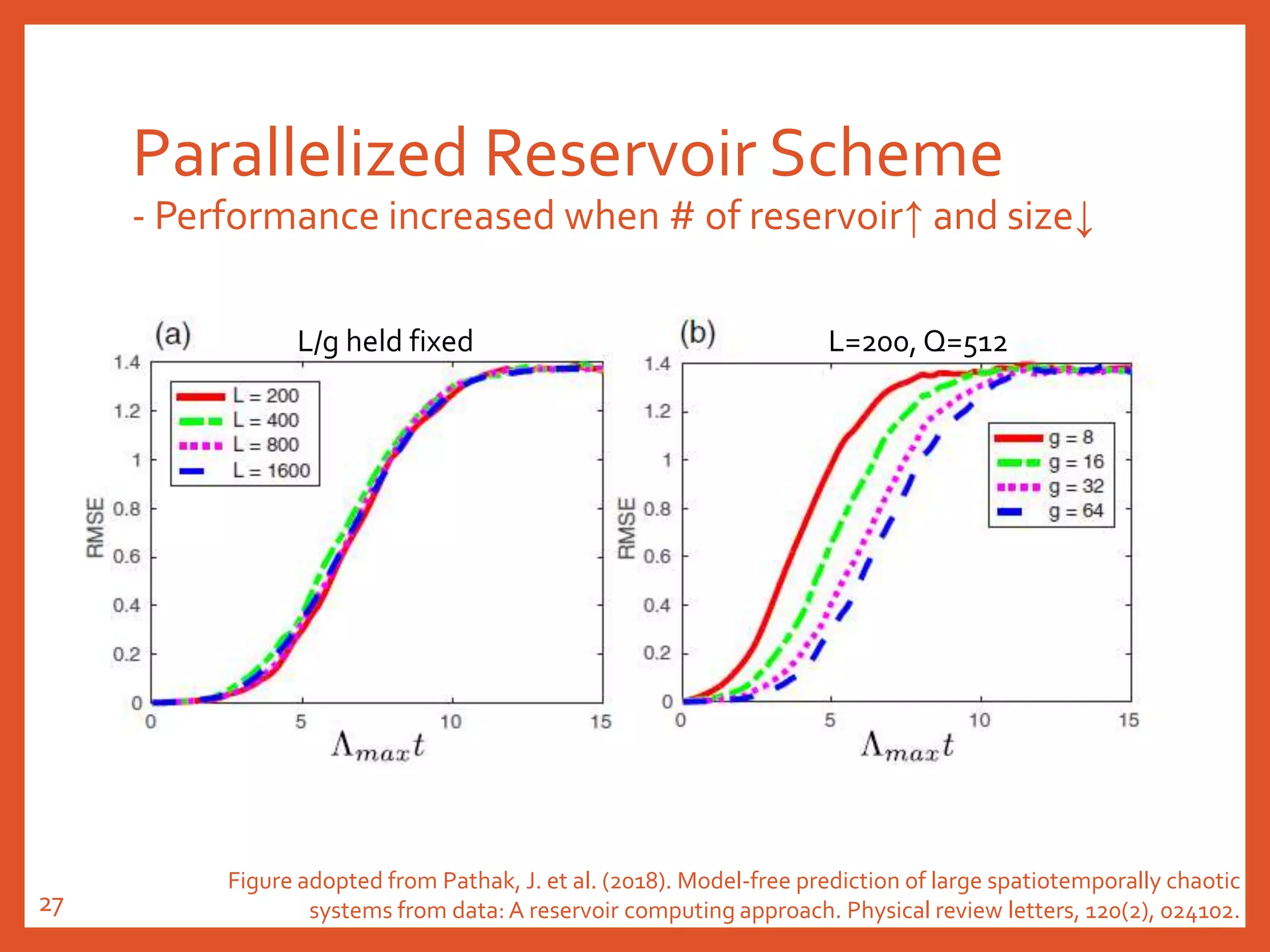
The document provides an introduction to reservoir computing from a dynamical system perspective, detailing the configuration of reservoirs, chaotic systems, and prediction mechanisms. It discusses the forecasting capabilities of reservoir computing specifically with the Kuramoto-Sivashinsky equation and highlights the fixed nature of certain parameters within the reservoir. The paper emphasizes the ability of reservoir computing to learn complex dynamical structures and make predictions based on chaotic data.

1. Introduction to Reservoir Computing
From a Dynamical System Perspective
Chia-Hsiang Kao
Oct. 19, 2019 @Mozilla Community SpaceTaipei

2. Outline
• Introduction to the configuration of reservoir
• Introduction to chaotic system
• Prediction of chaotic system using reservoir computing
• Mechanism of reservoir computing
2

3. Introduction to
the configuration of reservoir

4. Main Reference
• Pathak, J., Hunt, B., Girvan, M., Lu, Z., & Ott, E. (2018). Model-free
prediction of large spatiotemporally chaotic systems from data: A
reservoir computing approach. Physical review letters, 120(2), 024102.
• Pathak, J., Lu, Z., Hunt, B. R., Girvan, M., & Ott, E. (2017). Using machine
learning to replicate chaotic attractors and calculate Lyapunov
exponents from data. Chaos: An Interdisciplinary Journal of Nonlinear
Science, 27(12), 121102.
• Jaideep Pathak. MACHINE LEARNING FOR ANALYSIS OF HIGH-
DIMENSIONAL CHAOTIC SPATIOTEMPORAL DYNAMICAL SYSTEMS.
Princeton Plasma Physics Laboratory Theory Semina. (6/12/18)
4

5. Reservoir computing = a RNN with
𝑊 and 𝑈 fixed
Figure adopted from https://bit.ly/2J0mXjU5

6. Configuration of the Reservoir
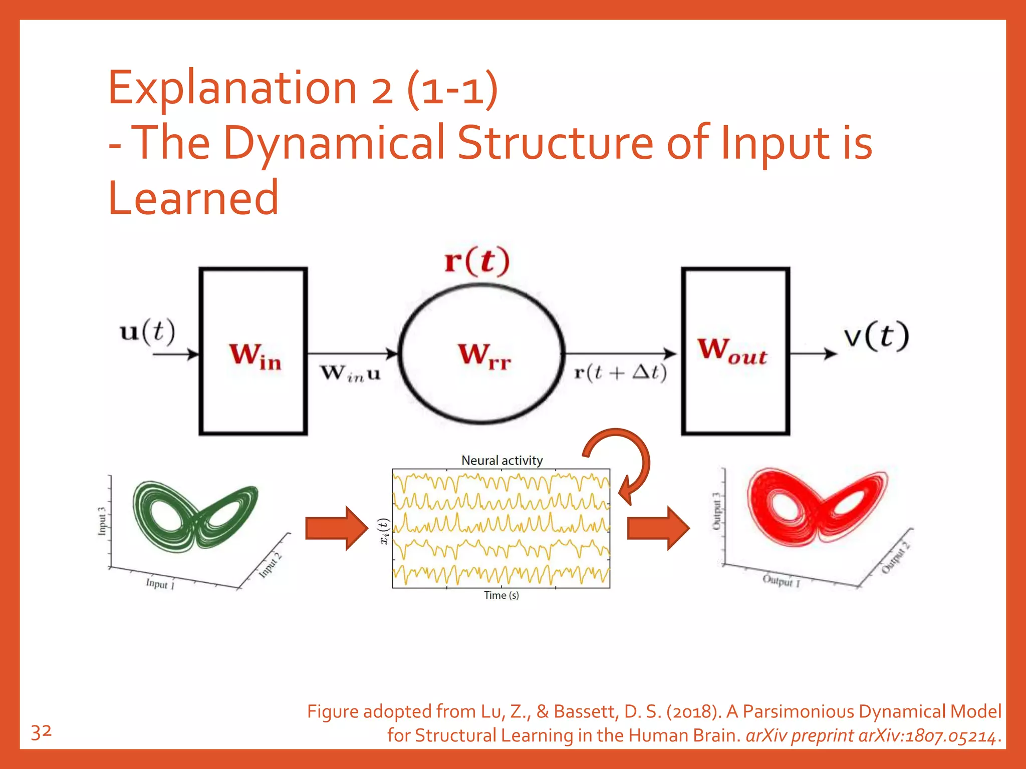
Input: 𝑢(𝑡)
Output: u(𝑡)
State of reservoir: r(𝑡)
𝒖(𝒕)
v(𝒕)
𝒓(𝒕)
𝑾 𝒓𝒓
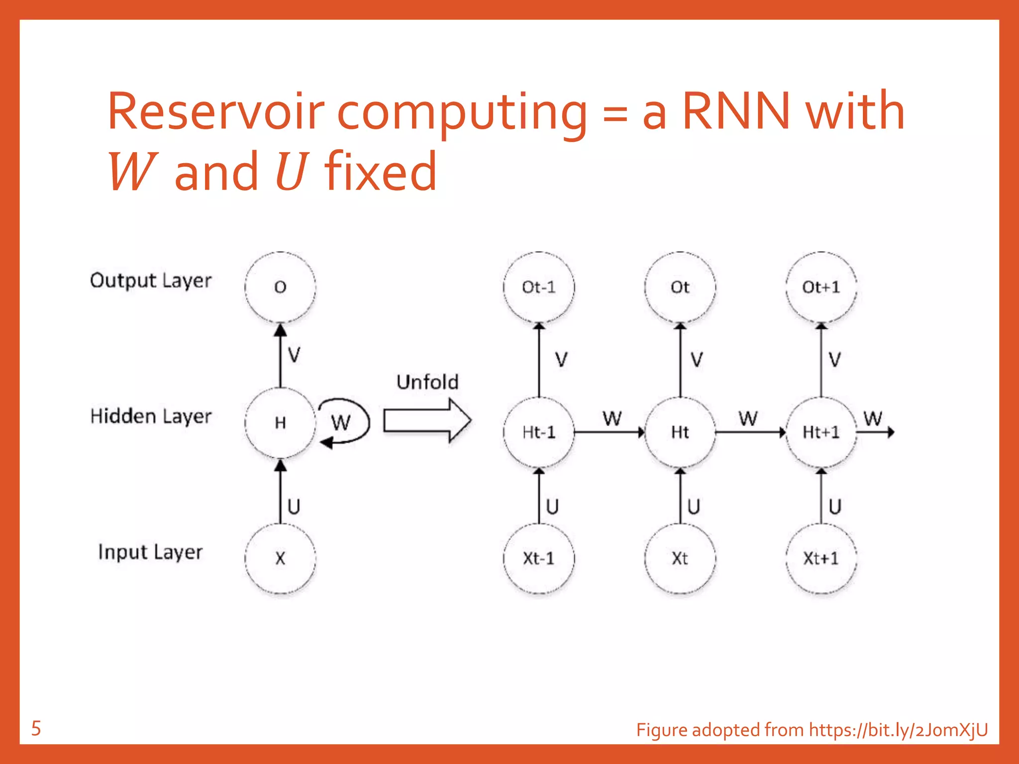
𝑊𝑖𝑛 and 𝑊𝑟𝑟 are fixed.
𝑊𝑜𝑢𝑡 is trainable!
Wrr: large, low-degree, directed,
random adjacent matrix
Update 𝑟(𝑡):
r t + Δt = tanh[𝐖𝐫𝐫r t + 𝐖𝐢𝐧u(t)] ,r(t)我會稱之為「reservoir的狀態」
Refer to Skibinsky-Gitlin et al. (2018, June). Cyclic Reservoir Computing with FPGA Devices for Efficient Channel
Equalization. In InternationalConference on Artificial Intelligence andSoftComputing (pp. 226-234). Springer, Cham.6

7. Hardware implementation using a
variety of physical systems
Figure adopted fromTanaka, G.,Yamane,T., Héroux, J. B., Nakane, R., Kanazawa, N.,
Takeda, S., ... & Hirose, A. (2019). Recent advances in physical reservoir computing:A
review. Neural Networks.
7

8. Introduction to chaotic
system

9. Blue point: (0,1,0)
Red point: (0,1.001,0)
Movie retrieved fromhttps://www.youtube.com/watch?v=8z_tSVeEFTA9

10. Motivation of this paper
An existing but unavailable
dynamical system
Short-term
forecasting &
long-term
dynamics
Reasonably accurate and
complete observational
data can be obtained
Figure adopted from Lu, Z., & Bassett, D. S. (2018). A Parsimonious Dynamical Model
for Structural Learning in the Human Brain. arXiv preprint arXiv:1807.05214.10

11. ~𝒙′(𝒕)
In this paper, a chaotic dynamical
system is concerned.
• We say a dynamical system is chaotic if two nearby
trajectories diverge exponentially.
• Consider separation 𝛿(𝑡) = 𝑥′
(𝑡) − 𝑥(𝑡).
• 𝛿 𝑡 ~𝑒 𝝀𝑡
𝛿 0
• Lyapunov exponent 𝝀 indicates predictability for a
dynamical system.
• 𝜆<0: distance decreases
• 𝜆>0: deviation grows exponentially
Figure adopted from https://bit.ly/35LZlJH11

12. In this paper, a chaotic dynamical
system is concerned.
• We say a dynamical system is chaotic if two nearby
trajectories diverge exponentially.
• Consider separation 𝛿(𝑡) = 𝑥′
(𝑡) − 𝑥(𝑡).
• 𝛿 𝑡 ~𝑒 𝝀𝑡
𝛿 0
• Lyapunov exponent 𝝀 indicates predictability for a
dynamical system.
• 𝜆<0: distance decreases
• 𝜆>0: deviation grows exponentially
• A dynamical system usually contains multiple
Lyapunov exponents.
Figure adopted fromJaideep Pathak. MACHINE LEARNING FORANALYSISOF HIGH-DIMENSIONALCHAOTIC
SPATIOTEMPORAL DYNAMICAL SYSTEMS. Princeton Plasma Physics LaboratoryTheory Semina. (6/12/18)12

13. Blue point: (0,1,0)
Red point: (0,1.001,0)
Movie retrieved fromhttps://www.youtube.com/watch?v=8z_tSVeEFTA13

14. Q: Can a traditional RNN or LSTM
learn to predict the future state of a
Lorenz system?
• RNN and LSTM can of course forecast the behavior of the Lorenz
system in short-term.
• Why or How?
• How about reservoir computing?
• Why or How?
14

15. Prediction of chaotic system
using reservoir computing

16. In this paper, the reservoir is built to
forecast the behavior of Kuramoto-
Sivashinsky Equation
• 𝑦𝑡 = −𝑦𝑦𝑡 − 𝑦𝑥𝑥 − 𝑦𝑥𝑥𝑥𝑥
gif retrieved from https://zhuanlan.zhihu.com/p/37730449
𝑥
16

17. In this paper, we want the reservoir
forecast the behavior of Kuramoto-
Sivashinsky Equation
• 𝑦𝑡 = −𝑦𝑦𝑡 − 𝑦𝑥𝑥 − 𝑦𝑥𝑥𝑥𝑥
• 𝑥 ∈ [0, 𝐿)
Figure adopted from Pathak, J. et al. (2017). Using machine learning to replicate chaotic attractors and calculate
Lyapunov exponents from data. Chaos: An Interdisciplinary Journal of Nonlinear Science, 27(12), 121102.17

18. In this paper, we want the reservoir
forecast the behavior of Kuramoto-
Sivashinsky Equation
• 𝑦𝑡 = −𝑦𝑦𝑡 − 𝑦𝑥𝑥 − 𝑦𝑥𝑥𝑥𝑥
• 𝐱 ∈ [𝟎, 𝐋)
L
12 13.5
36 100
Figure adopted from Edson, R. A., Bunder, J. E., Mattner,T.W., & Roberts, A. J. (2019). Lyapunov
exponents of the Kuramoto–Sivashinsky PDE.TheANZIAM Journal, 61(3), 270-285.18

19. In this paper, we want the reservoir
forecast the behavior of Kuramoto-
Sivashinsky Equation
• 𝑦𝑡 = −𝑦𝑦𝑡 − 𝑦𝑥𝑥 − 𝑦𝑥𝑥𝑥𝑥
• 𝑥 ∈ [0, 𝐿)
• 𝐲 𝐱 + 𝑳 = 𝐲(𝐱)
Figure adopted from Pathak, J. et al. (2017). Using machine learning to replicate chaotic attractors and calculate
Lyapunov exponents from data. Chaos: An Interdisciplinary Journal of Nonlinear Science, 27(12), 121102.19

20. Predict the Behavior of
Kuramoto-Sivashinsky Equation (4)
• 𝑦𝑡 = −𝑦𝑦𝑡 − 𝑦𝑥𝑥 − 𝑦𝑥𝑥𝑥𝑥
• 𝑥 ∈ [0, 𝐿)
• 𝑦 𝑥 + 𝐿 = 𝑦(𝑥)
• Divided [0,L) into Q parts such that
• 𝑢 𝑡 = 𝑦 Δ𝑥, 𝑡 , 𝑦 2Δ𝑥, 𝑡 , … , 𝑦(QΔ𝑥, 𝑡) 𝑇
• 𝑸 =
𝑳
𝚫𝒙
is the input size of reservoir
Δ𝑥
t
Figure adopted from Pathak, J. et al. (2017). Using machine learning to replicate chaotic attractors and calculate
Lyapunov exponents from data. Chaos: An Interdisciplinary Journal of Nonlinear Science, 27(12), 121102.20

21. Configuration of the Reservoir in the Paper
𝐫 𝒕
r t + Δt = tanh[𝐖𝐫𝐫 ⋅ r t + 𝐖𝐢𝐧 ⋅ u(t)] ,
v t = 𝐖𝐨𝐮𝐭 ⋅ r t
𝐖𝐢𝐧
𝐖𝒐𝒖𝒕𝐖𝐫𝐫
v 𝑡
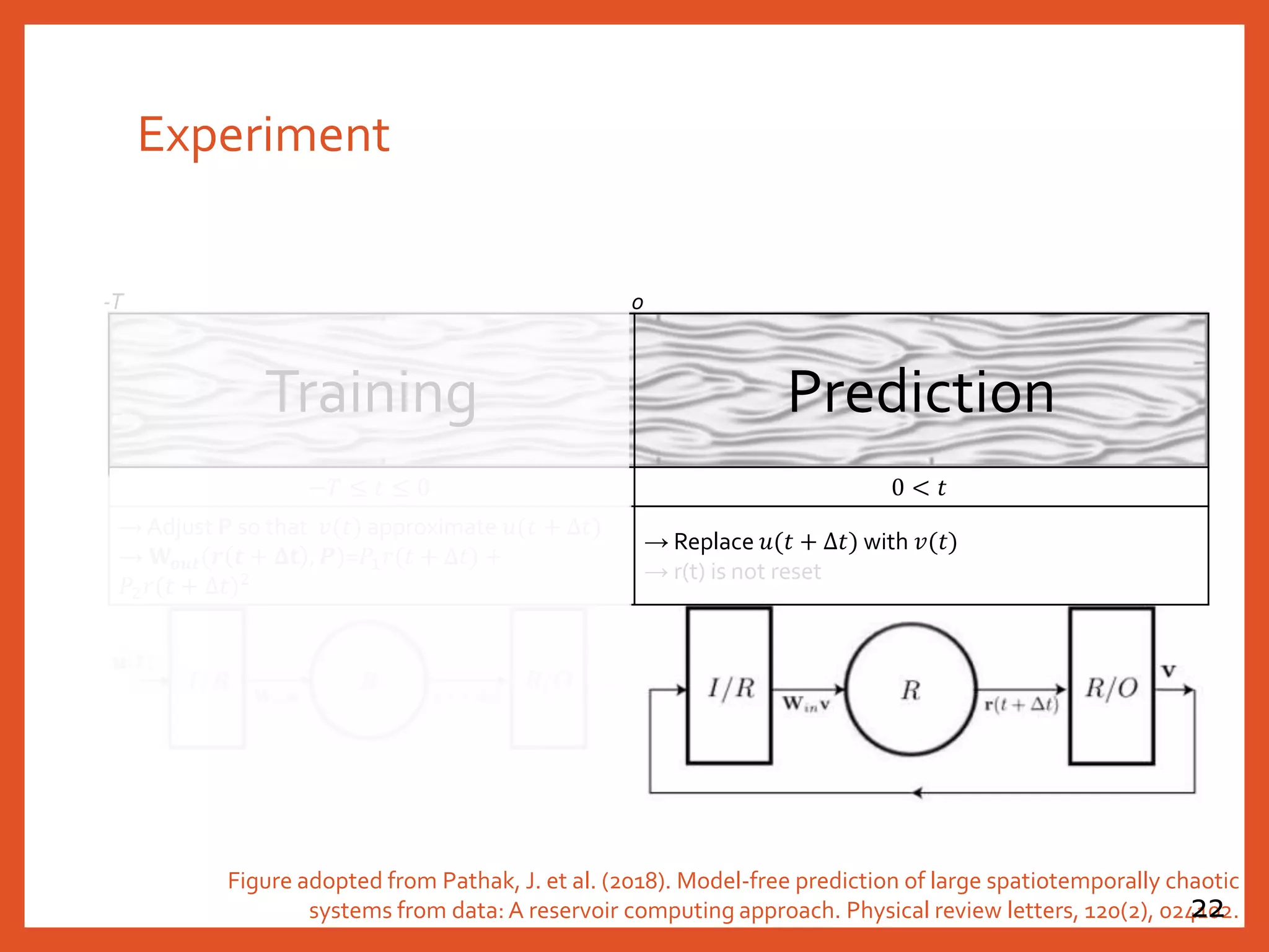
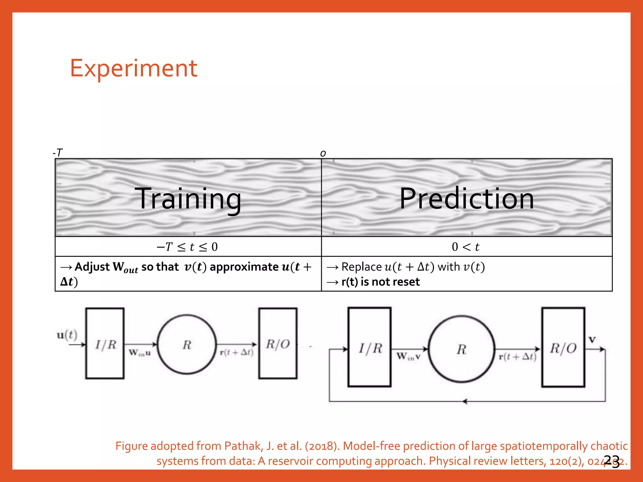
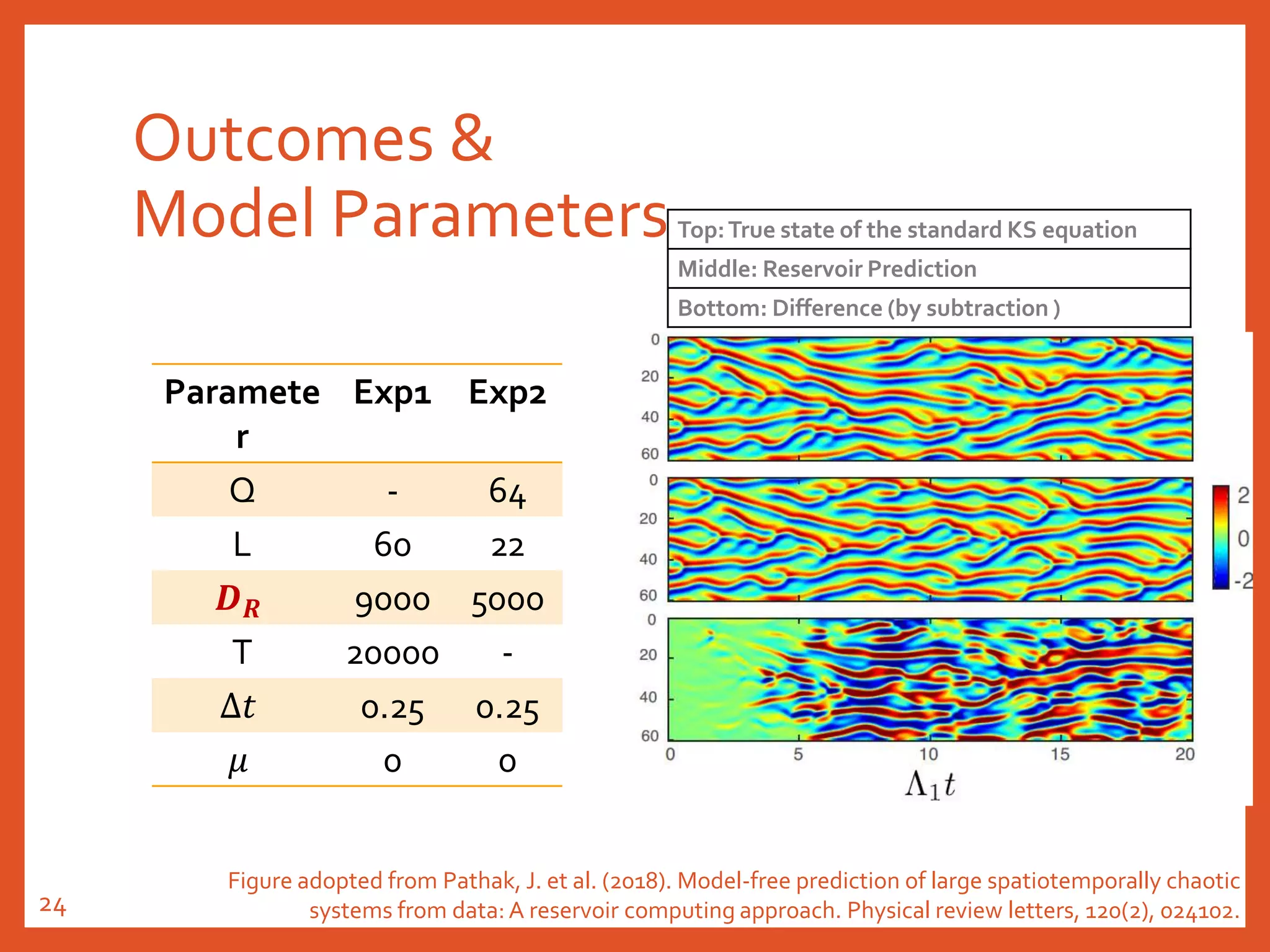
Figure adopted from Pathak, J. et al. (2018). Model-free prediction of large spatiotemporally chaotic
systems from data: A reservoir computing approach. Physical review letters, 120(2), 024102.21

22. Experiment
Training Prediction
−𝑇 ≤ 𝑡 ≤ 0 0 < 𝑡
→Adjust P so that 𝑣(𝑡) approximate 𝑢(𝑡 + Δ𝑡)
→ 𝐖𝒐𝒖𝒕(𝒓 𝒕 + 𝚫𝐭 , 𝑷)=𝑃1 𝑟(𝑡 + Δ𝑡) +
𝑃2 𝑟(𝑡 + Δ𝑡)2
→ Replace 𝑢(𝑡 + Δ𝑡) with 𝑣(𝑡)
→ r(t) is not reset
0-T
Figure adopted from Pathak, J. et al. (2018). Model-free prediction of large spatiotemporally chaotic
systems from data: A reservoir computing approach. Physical review letters, 120(2), 024102.22

23. Experiment
Training Prediction
−𝑇 ≤ 𝑡 ≤ 0 0 < 𝑡
→ Adjust 𝐖𝒐𝒖𝒕 so that 𝒗(𝒕) approximate 𝒖(𝒕 +
𝚫𝒕)
→ Replace 𝑢(𝑡 + Δ𝑡) with 𝑣(𝑡)
→ r(t) is not reset
0-T
Figure adopted from Pathak, J. et al. (2018). Model-free prediction of large spatiotemporally chaotic
systems from data: A reservoir computing approach. Physical review letters, 120(2), 024102.23

24. Outcomes &
Model ParametersTop:True state of the standard KS equation
Middle: Reservoir Prediction
Bottom: Difference (by subtraction )
Paramete
r
Exp1 Exp2
Q - 64
L 60 22
𝑫 𝑹 9000 5000
T 20000 -
Δ𝑡 0.25 0.25
𝜇 0 0
Figure adopted from Pathak, J. et al. (2018). Model-free prediction of large spatiotemporally chaotic
systems from data: A reservoir computing approach. Physical review letters, 120(2), 024102.24

25. An interesting observation
• It seems that the reservoir is trapped.
25

26. Outpu
t
Extension – Parallelized Reservoir
Scheme
• 𝑅𝑖 has its own 𝐴𝑖 (adjacency matrix), 𝑟𝑖 (internal state) and 𝑊𝑖𝑛,𝑖 (input weights).
• 𝑅𝑖 receives additional input from continuous variables. ⇒ ℎ𝑖
• Input 𝑢(𝑡) is split into 𝑔 group, each group consisting of 𝑞 variables. ⇒
𝑄 = 𝑔 ⋅ 𝑞
Input
𝑔𝑖−1 𝑔𝑖+1
Figure adopted from Pathak, J. et al. (2018). Model-free prediction of large spatiotemporally chaotic
systems from data: A reservoir computing approach. Physical review letters, 120(2), 024102.26

27. Parallelized Reservoir Scheme
- Performance increased when # of reservoir↑ and size↓
L/g held fixed L=200, Q=512
Figure adopted from Pathak, J. et al. (2018). Model-free prediction of large spatiotemporally chaotic
systems from data: A reservoir computing approach. Physical review letters, 120(2), 024102.27

28. Explanation for
reservoir computing

29. Explanation 1
- Projection onto High-dimension
Subspace ?
Figure adopted from https://bit.ly/32trwuX30

30. Explanation 2 (1-1)
-The Dynamical Structure of Input is
Learned
Figure adopted from Lu, Z., & Bassett, D. S. (2018). A Parsimonious Dynamical Model
for Structural Learning in the Human Brain. arXiv preprint arXiv:1807.05214.32

31. Explanation 2 (1-2)
-The Dynamical Structure of Input is
Learned
How, when and where is the structure learned?
Especially when 𝑾 𝒓𝒓 and 𝑾𝒊𝒏 are fixed.
Figure adopted from Lu, Z., & Bassett, D. S. (2018). A Parsimonious Dynamical Model
for Structural Learning in the Human Brain. arXiv preprint arXiv:1807.05214.33

32. Explanation 2 (1-2)
-The Dynamical Structure of Input is
Learned
(x,y,z) (x,y’,z’)
𝑥 = 𝜎(𝑦 − 𝑧)
𝑦 = −𝑥𝑧 + 𝑟𝑥 − 𝑦 𝑦′ = −𝑥𝑧′ + 𝑟𝑥 − 𝑦′
𝑧 = 𝑥𝑦 − 𝑏𝑧 𝑧′ = 𝑥𝑦′ − 𝑏𝑧′
Figure adopted from Pecora, L. M., &Carroll, T. L. (2015). Synchronization of chaotic
systems. Chaos: An Interdisciplinary Journal of Nonlinear Science, 25(9), 097611.34

33. Explanation 2 (1-4)
-The Dynamical Structure of Input is
Learned - A simple and parsimonious explanation
External System
(drive)
Central System
(response)
Space ℝ 𝑛
ℝ 𝑁
Chaotic
attractor
𝐴k 𝑃k
Input
trajectory
𝑠(𝑡) 𝑥(𝑡)
𝜑(⋅)
𝜙(⋅)
35

34. Explanation 2 (2-1)
-The Dynamical Structure of Input is
Learned
• 蓄水池网络具有的一种能力是， 如果你给它一个复杂的时间序列输入
（I）， 比如股市的变化， 它可以自动的抽取出这种变化背后的独立性
因子，并在一定程度模拟出真实过程的动力关系（因为其自身存在足
够丰富的动力关系， 以至于非常容易和真实的系统进行匹配）。 听着
有点像PCA，但是PCA是线性的不包含时间， 而这里是一个非线性时间
依赖的系统， 复杂性不可同日而语。
• 多么复杂的波动背后催生它的因素不一定很复杂， 比如洛伦茨吸引子
背后就仅仅是一个三维系统。当这个波动输入到蓄水池网络里以后，
蓄水池网络可以找寻到这种复杂背后的根基，并对这个信号的发展走
势进行预测。
作者：许铁-巡洋舰科技
網址：https://www.zhihu.com/question/265476523/answer/74765341537

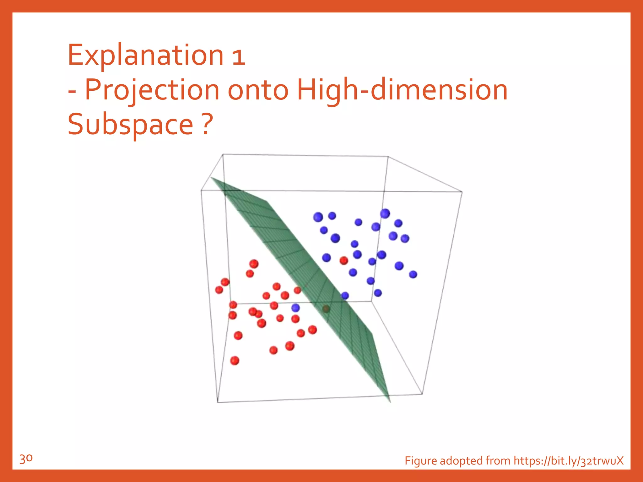
35. Explanation 2 (2-2)
-The Dynamical Structure of Input is
Learned
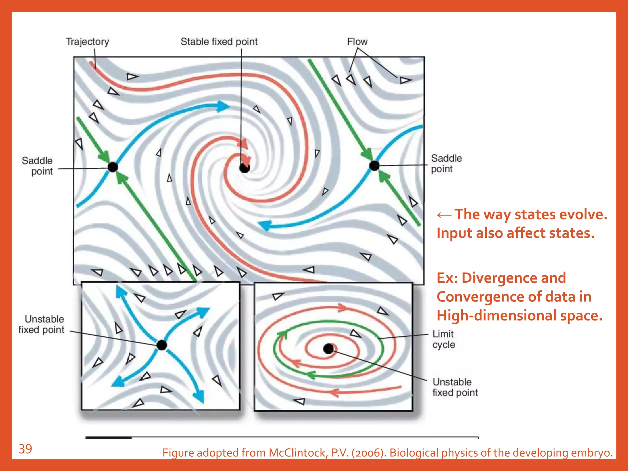
• 在各类复杂的动力学形式里， 我们看到，无论是稳定定点， 极限环，
鞍点，还是线性吸引子，事实上都是对世界普遍存在的信息流动形式
的通用表达。
• 可以用它表达信息的提取和加工， 甚至某种程度的逻辑推理（决策），
那么只要我们能够掌握一种学习形式有效的改变这个随机网络的连接，
我们就有可能得到我们所需要的任何一种信息加工过程。
• 用几何语言说就是，在随机网络的周围， 存在着从毫无意义的运动到
通用智能的几乎所有可能性， 打开这些可能的过程如同[外在环境]对
随机网络进行一个微扰， 而这个微扰通常代表了某种网络和外在环境
的耦合过程（学习）， 当网络的动力学在低维映射里包含了真实世界
的动力学本身， 通常学习就成功了。
作者：许铁-巡洋舰科技
網址：https://www.zhihu.com/question/265476523/answer/74765341538

36. Figure adopted from McClintock, P.V. (2006). Biological physics of the developing embryo.
←The way states evolve.
Input also affect states.
Ex: Divergence and
Convergence of data in
High-dimensional space.
39

37. Information is processed by extremely
complex but surprisingly stereotypic
microcircuits
Figure adopted from Mountcastle,V. B. (1997).The columnar organization of the neocortex. Brain: a
journal of neurology, 120(4), 701-722. & Habenschuss, S., Jonke, Z., & Maass,W. (2013). Stochastic
computations in cortical microcircuit models. PLoS computational biology, 9(11), e1003311.40

38. Credits and Reference
• 【Template】SlidesCarnival
• Real-Time ComputingWithout Stable States: A New Framework for Neural Computation
Based on Perturbations
• Recent Advances in Physical Reservoir Computing: A Review
• Model-Free Prediction of Large Spatiotemporally Chaotic Systems from Data: A Reservoir
Computing Approach
• Using machine learning to replicate chaotic attractors and calculate Lyapunov exponents
from data
• 【Seminar】 Machine learning for analysis of high-dimensional chaotic statiotemporal
dynamical systems
• Lyapunov exponents of the Kuramoto–Sivashinsky PDE
• 【知乎】神经网络的参数都是随机的，有的效果很好，有的效果很差，这真的不是玄
学吗？, https://www.zhihu.com/question/265476523/answer/747653415
• A Parsimonious Dynamical Model for Structural Learning in the Human Brain.
• Pecora, L. M., & Carroll,T. L. (2015). Synchronization of chaotic systems. Chaos: An
Interdisciplinary Journal of Nonlinear Science, 25(9), 097611.
41

39. Figure
• Cyclic Reservoir Computing with FPGA Devices for Efficient Channel Equalization.
• http://ycpcs.github.io/cs360-spring2015/lectures/lecture15.html
• https://medium.com/ai-journal/lstm-gru-recurrent-neural-networks-81fe2bcdf1f9
• https://2e.mindsmachine.com/asf05.01.html
• The columnar organization of the neocortex.
• https://juliadynamics.github.io/DynamicalSystems.jl/latest/chaos/lyapunovs/
• https://www.youtube.com/watch?v=8z_tSVeEFTA
42

40. Thank you for your attention