Downloaded 16 times


![Data Partitioning
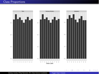
We created a 70/30 split of the data based on the distributions of class labels for
our training and validation set.
training_index <- createDataPartition(y = training[,1],
p = .7,
list = FALSE)
training <- training[training_index,]
validation <- training[-training_index,]
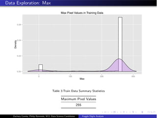
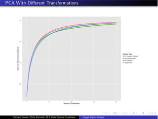
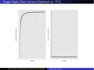
100 covariates were kept due to explaining approximately 95% of variation in the
data, and for the ease of presentation.
dim(training)
## [1] 29404 101
dim(validation)
## [1] 8821 101
Zachary Combs, Philip Remmele, M.S. Data Science Candidates Kaggle Digits Analysis](https://image.slidesharecdn.com/kaggledigitsanalysisfinalfc1-150831014236-lva1-app6892/85/Kaggle-digits-analysis_final_fc-14-320.jpg)
![Linear Discriminant Analysis
Discriminant Function
δk (x) = xT
Σ−1
µk −
1
2
µT
k Σ−1
µk + logπk
Estimating Class Probabilities
Pr(Y = k|X = x) =
πk e
δk
K
l=1 πl e
δ l (x)
Assigning x to the class with the largest discriminant score δk (x) will result in the
highest probability for that classification. [James, 2013]
Zachary Combs, Philip Remmele, M.S. Data Science Candidates Kaggle Digits Analysis](https://image.slidesharecdn.com/kaggledigitsanalysisfinalfc1-150831014236-lva1-app6892/85/Kaggle-digits-analysis_final_fc-17-320.jpg)
![Model Fitting: LDA
ind - seq(10,100,10)
lda_Ctrl - trainControl(method = repeatedcv, repeats = 3,
classProbs = TRUE,
summaryFunction = defaultSummary)
accuracy_measure_lda - NULL
ptm - proc.time()
for(i in 1:length(ind)){
lda_Fit - train(label ~ ., data = training[,1:(ind[i]+1)],
method = lda,
metric = Accuracy,
maximize = TRUE,
trControl = lda_Ctrl)
accuracy_measure_lda[i] - confusionMatrix(validation$label,
predict(lda_Fit,
validation[,2:(ind[i]+1)]))$overall[1]
}
proc.time() - ptm
## user system elapsed
## 22.83 2.44 129.86
Zachary Combs, Philip Remmele, M.S. Data Science Candidates Kaggle Digits Analysis](https://image.slidesharecdn.com/kaggledigitsanalysisfinalfc1-150831014236-lva1-app6892/85/Kaggle-digits-analysis_final_fc-18-320.jpg)

![Quadratic Discriminant Analysis
Discriminant Function
δk (x) = −
1
2
(x − µk )T
Σ−1
k (x − µk ) + logπk
Estimating Class Probabilities
Pr(Y = k|X = x) =
πk fk (x)
K
l=1 πl fl (x)
While fk (x) are Gaussian densities with different covariance matrix
for each class
we obtain a Quadratic Discriminant Analysis. [James, 2013]
Zachary Combs, Philip Remmele, M.S. Data Science Candidates Kaggle Digits Analysis](https://image.slidesharecdn.com/kaggledigitsanalysisfinalfc1-150831014236-lva1-app6892/85/Kaggle-digits-analysis_final_fc-25-320.jpg)
![Model Fitting: QDA
qda_Ctrl - trainControl(method = repeatedcv, repeats = 3,
classProbs = TRUE,
summaryFunction = defaultSummary)
accuracy_measure_qda - NULL
ptm - proc.time()
for(i in 1:length(ind)){
qda_Fit - train(label ~ ., data = training[,1:(ind[i]+1)],
method = qda,
metric = Accuracy,
maximize = TRUE,
trControl = lda_Ctrl)
accuracy_measure_qda[i] - confusionMatrix(validation$label,
predict(qda_Fit,
validation[,2:(ind[i]+1)]))$overall[1]
}
proc.time() - ptm
## user system elapsed
## 20.89 2.16 66.20
Zachary Combs, Philip Remmele, M.S. Data Science Candidates Kaggle Digits Analysis](https://image.slidesharecdn.com/kaggledigitsanalysisfinalfc1-150831014236-lva1-app6892/85/Kaggle-digits-analysis_final_fc-26-320.jpg)


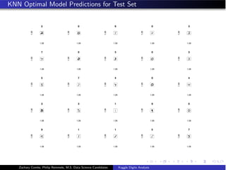
![KNN: Optimal Model Fitting
knn_Ctrl - trainControl(method = repeatedcv, repeats = 3,
classProbs = TRUE,
summaryFunction = defaultSummary)
knn_grid - expand.grid(k=c(1,2,3,4,5))
knn_Fit_opt - train(label~., data = training[,1:(knn_opt+1)],
method = knn,
metric = Accuracy,
maximize = TRUE,
tuneGrid = knn_grid,
trControl = knn_Ctrl)
accuracy_measure_knn_opt - confusionMatrix(validation$label,
predict(knn_Fit_opt,
validation[,2:(knn_opt+1)]))
Zachary Combs, Philip Remmele, M.S. Data Science Candidates Kaggle Digits Analysis](https://image.slidesharecdn.com/kaggledigitsanalysisfinalfc1-150831014236-lva1-app6892/85/Kaggle-digits-analysis_final_fc-36-320.jpg)


![Random Forest
”A random forest is a classifier consisting of a collection of tree-structured
classifiers {h(x, θk ), k = 1} where the {θk } are independent identically
distributed random vectors and each tree casts a unit vote for the most
popular class input x.” [Breiman, 2001]
Zachary Combs, Philip Remmele, M.S. Data Science Candidates Kaggle Digits Analysis](https://image.slidesharecdn.com/kaggledigitsanalysisfinalfc1-150831014236-lva1-app6892/85/Kaggle-digits-analysis_final_fc-42-320.jpg)
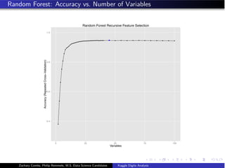
![RF Model Fitting: Recursive Feature Selection
subsets - c(1:40,seq(45,100,5)) # vector of variable subsets
# for recursive feature selection
ptm - proc.time() # starting timer for code execution
ctrl - rfeControl(functions = rfFuncs, method = repeatedcv,
number = 3, verbose = FALSE,
returnResamp = all, allowParallel = FALSE)
rfProfile - rfe(x = training[,-1],
y = as.factor(as.character(training$label)),
sizes = subsets, rfeControl = ctrl)
rf_opt - rfProfile$optVariables
proc.time() - ptm
## user system elapsed
## 7426.48 64.87 7491.48
Zachary Combs, Philip Remmele, M.S. Data Science Candidates Kaggle Digits Analysis](https://image.slidesharecdn.com/kaggledigitsanalysisfinalfc1-150831014236-lva1-app6892/85/Kaggle-digits-analysis_final_fc-43-320.jpg)
![Conditional Inference Tree
General Recursive Partitioning Tree
1. Perform an exhaustive search over all possible splits
2. Maximize information measure of node impurity
3. Select covariate split that maximized this measure
CTREE
1. In each node the partial hypotheses Hj
o : D(Y |Xj ) = D(Y ) is tested against the
global null hypothesis of H0 =
m
j=1 Hj
0.
2. If the global hypothesis can be rejected then the association between Y and each
of the covariates Xj , j = 1..., m is measured by P-value.
3. If we are unable to reject H0 at the specified α then recursion is stopped.
[Hothorn, 2006]
Zachary Combs, Philip Remmele, M.S. Data Science Candidates Kaggle Digits Analysis](https://image.slidesharecdn.com/kaggledigitsanalysisfinalfc1-150831014236-lva1-app6892/85/Kaggle-digits-analysis_final_fc-49-320.jpg)
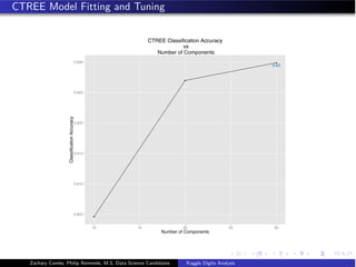
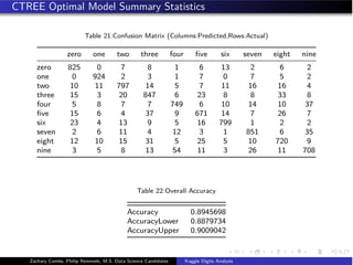
![CTREE: Optimal Model Fitting
ctree_Ctrl - trainControl(method = repeatedcv, repeats = 3,
classProbs = TRUE,
summaryFunction = defaultSummary)
ctree_Fit_opt - train(label~., data = training[,1:(ctree_opt+1)],
method = ctree,
metric = Accuracy,
tuneLength = 5,
maximize = TRUE,
trControl = ctree_Ctrl)
accuracy_measure_ctree_opt - confusionMatrix(validation$label,
predict(ctree_Fit_opt,
validation[,2:(ctree_opt+1)]))
Zachary Combs, Philip Remmele, M.S. Data Science Candidates Kaggle Digits Analysis](https://image.slidesharecdn.com/kaggledigitsanalysisfinalfc1-150831014236-lva1-app6892/85/Kaggle-digits-analysis_final_fc-51-320.jpg)

![Multinomial Logistic Regression
Class Probabilities
Pr(Y = k|X = x) =
eβ0k +β1k X1+...+βpk Xp
K
l=1 eβ0l +β1l X1+...+βpl Xp
Logistic Regression Model generalized for problems containing more than two classes.
[James, 2013]
Zachary Combs, Philip Remmele, M.S. Data Science Candidates Kaggle Digits Analysis](https://image.slidesharecdn.com/kaggledigitsanalysisfinalfc1-150831014236-lva1-app6892/85/Kaggle-digits-analysis_final_fc-56-320.jpg)
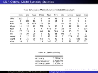


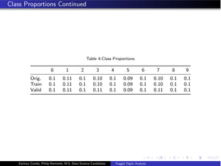
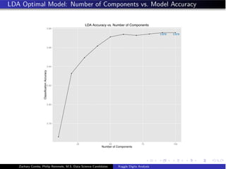
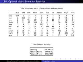
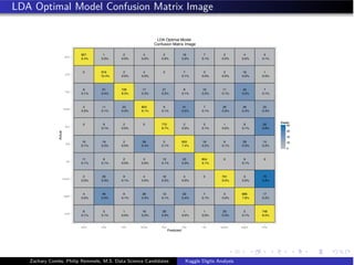
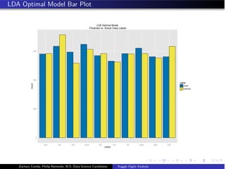
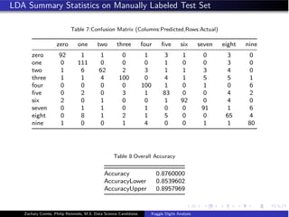
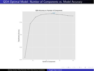
- The document analyzes the Kaggle Digits dataset using linear discriminant analysis (LDA) to classify handwritten digits - LDA accuracy was evaluated using repeated cross-validation as the number of components was increased from 10 to 100 - The optimal LDA model used 100 components and achieved an accuracy of 87.6% on the validation data - This model was then used to predict labels on the test set, achieving similar accuracy percentages for each digit class