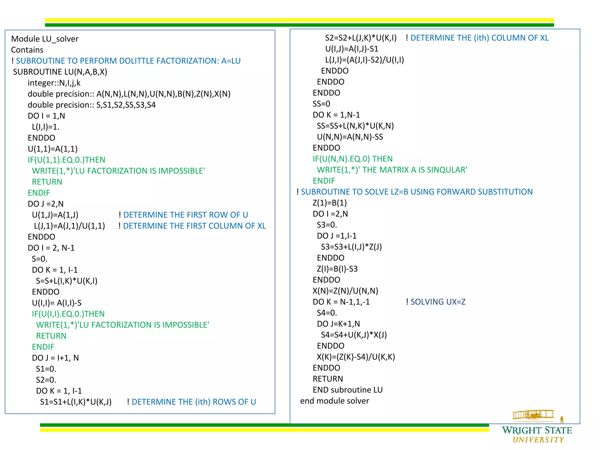
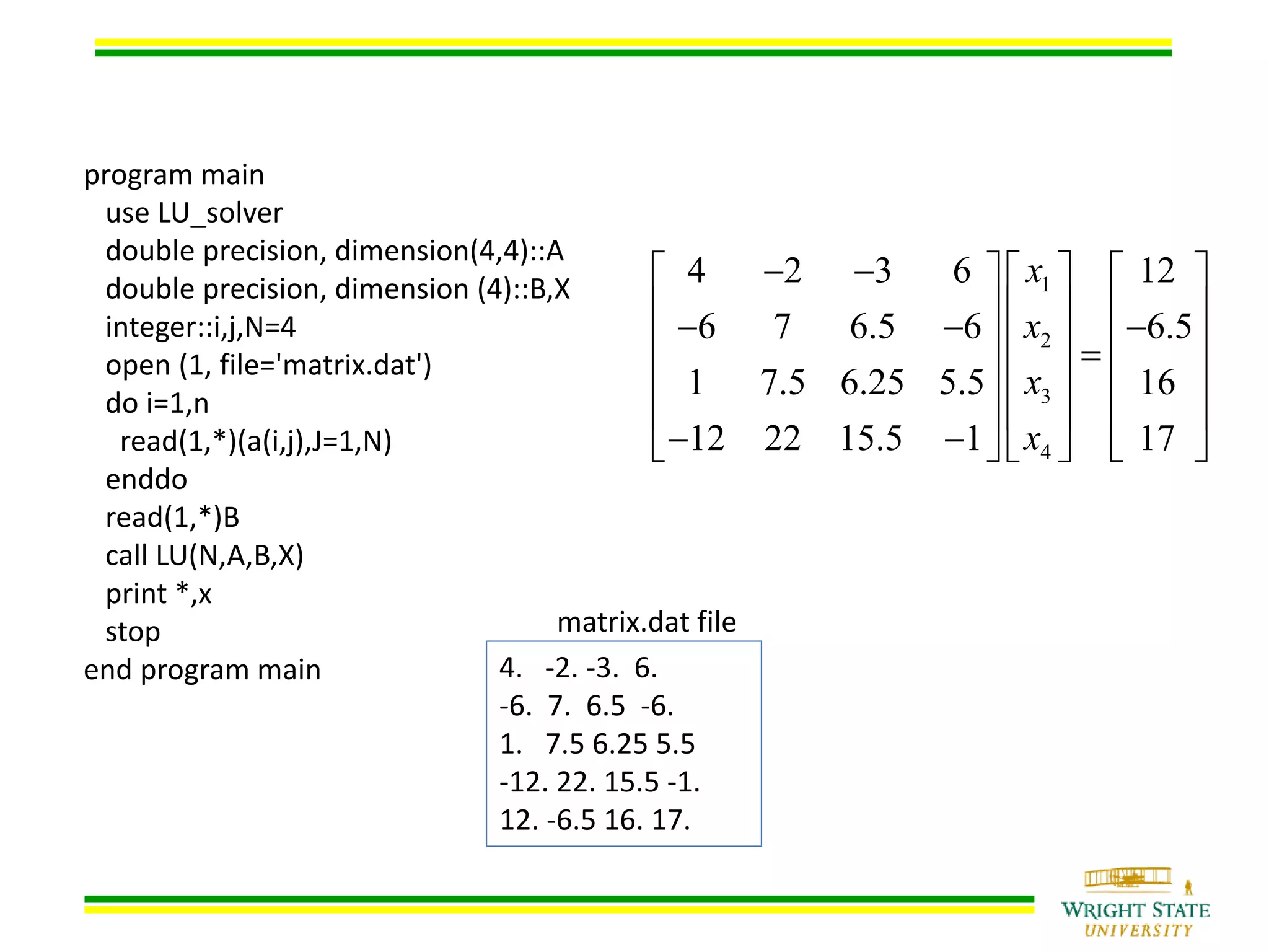
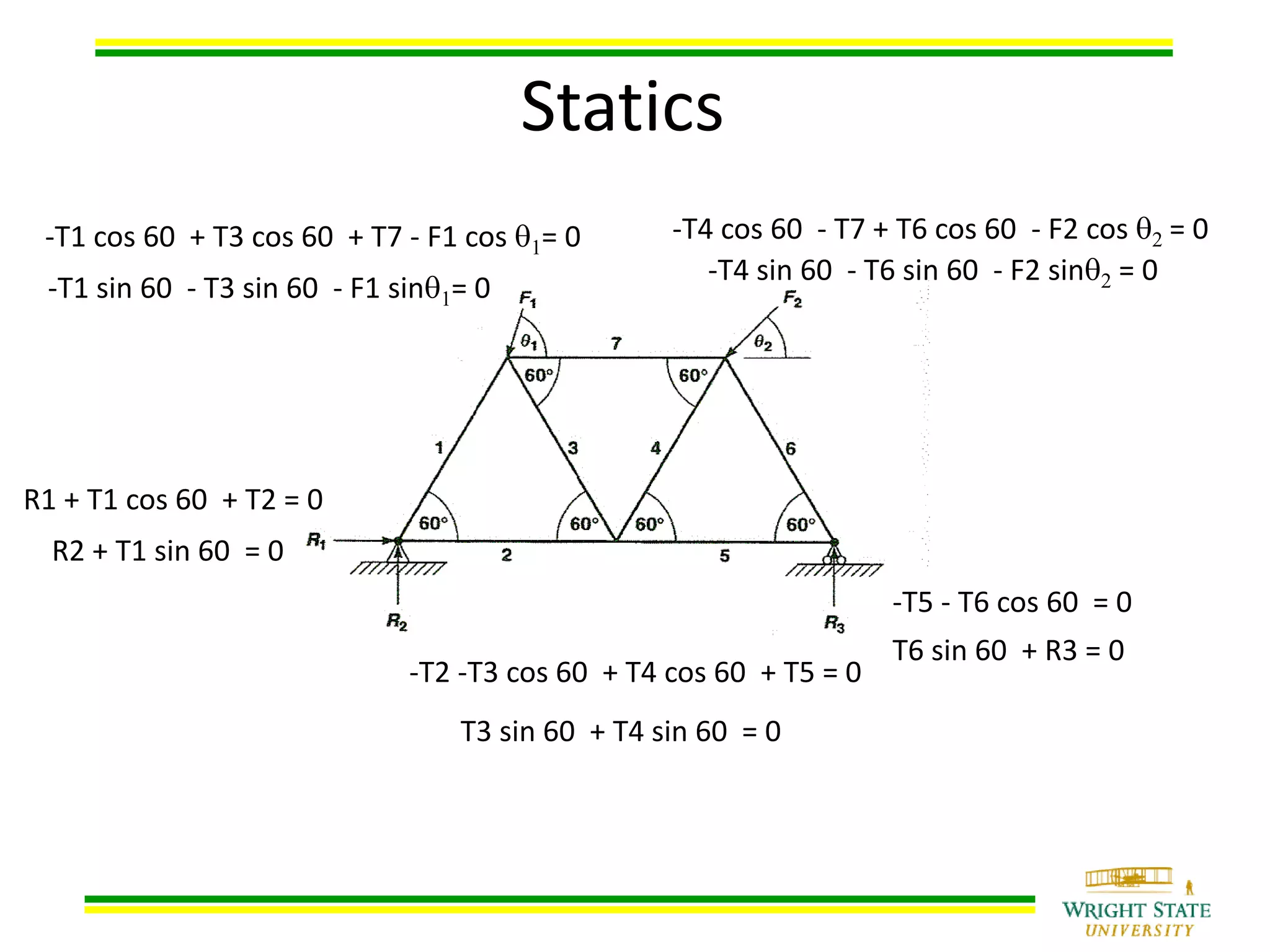
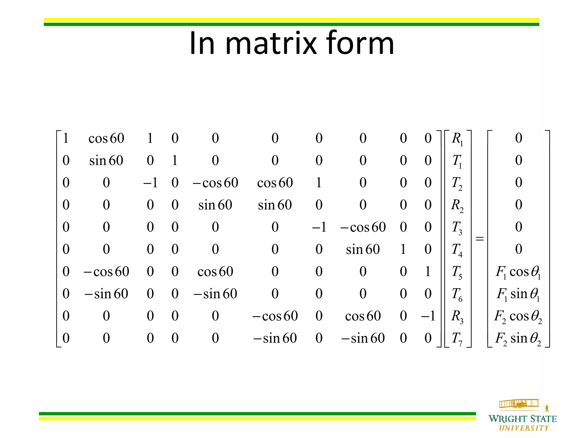
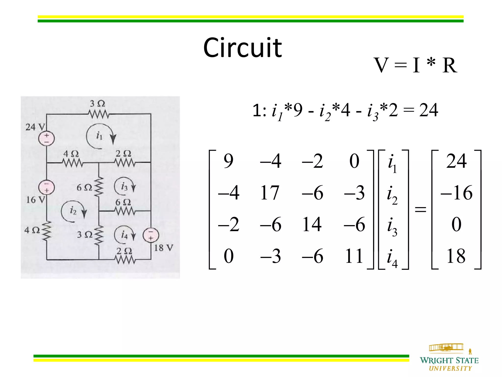
This document provides information about solving systems of equations using LU decomposition. It begins with an example system of equations and shows the steps to decompose the coefficient matrix [A] into lower [L] and upper [U] triangular matrices. It then explains that solving the original system involves first solving [L][Z]=[B] for [Z], then [U][X]=[Z] for [X]. The document provides an example using a 4x4 matrix to decompose it into [L] and [U], then uses the matrices to solve the system.

1. ME4010 Computational Methods for
Mechanical Engineering
Chapter 4 Solution of system of equations
Instructor: Nikolai V. Priezjev
Office: 430 Russ Engineering Center
Phone: 937-775-3214
Email: nikolai.priezjev@wright.edu
The course is adopted from Prof. Huang at WSU

2.  
 
)(
2)(
2
23332
2
3
1222322
2
2
111212
2
1
xxkgmx
dt
d
m
xxkgmxxkx
dt
d
m
kxgmxxkx
dt
d
m



1 2 1
1 2 3 2
2 3 3
3 2 0
2 3
0
kx kx m g
kx kx kx m g
kx kx m g
  
   
  
The steady state equations are:
1 1
2 2
3 3
3 2 0
2 3
0
k k x m g
k k k x m g
k k x m g
     
            
          
In matrix form:
Dynamics

3. Statics
R1 + T1 cos 60 + T2 = 0
R2 + T1 sin 60 = 0
-T2 -T3 cos 60 + T4 cos 60 + T5 = 0
T3 sin 60 + T4 sin 60 = 0
-T5 - T6 cos 60 = 0
T6 sin 60 + R3 = 0
-T1 cos 60 + T3 cos 60 + T7 - F1 cos = 0
-T1 sin 60 - T3 sin 60 - F1 sin= 0
-T4 cos 60 - T7 + T6 cos 60 - F2 cos  = 0
-T4 sin 60 - T6 sin 60 - F2 sin = 0

4. In matrix form
1 cos60 1 0 0 0 0 0 0 0
0 sin60 0 1 0 0 0 0 0 0
0 0 1 0 cos60 cos60 1 0 0 0
0 0 0 0 sin60 sin60 0 0 0 0
0 0 0 0 0 0 1 cos60 0 0
0 0 0 0 0 0 0 sin60 1 0
0 cos60 0 0 cos60 0 0 0 0 1
0 sin60 0 0 sin60 0 0 0 0 0
0 0 0 0 0 cos60 0 cos60 0 1
0 0 0 0 0 sin60 0 sin60 0 0
 
 
 
  
 
 
  
 

 

 
  
   
1
1
2
2
3
4
5 1 1
6 1 1
3 2 2
7 2 2
0
0
0
0
0
0
cos
sin
cos
sin
R
T
T
R
T
T
T F
T F
R F
T F




   
   
   
   
   
   
   
    
   
   
   
   
   
   
      

5. Circuit
1
2
3
4
9 4 2 0 24
4 17 6 3 16
2 6 14 6 0
0 3 6 11 18
i
i
i
i
      
           
      
    
     
V = I * R
1: i1*9 - i2*4 - i3*2 = 24

6. Method
[A] = [L][U]
where
[L] = lower triangular matrix
[U] = upper triangular matrix
LU Decomposition
Given [A][X] = [B]
1. Decompose [A] into [L] and [U]
2. Solve [L][Z] = [B] for [Z]
3. Solve [U][X] = [Z] for [X]

7. Method: [A] Decomposes to [L] and [U]
    





















33
2322
131211
3231
21
00
0
1
01
001
u
uu
uuu
ULA


[U] is the same as the coefficient matrix at the end of the forward elimination step.
[L] is obtained using the multipliers that were used in the forward elimination process

8. Finding the [U] matrix
Using the Forward Elimination Procedure of Gauss Elimination
112144
1864
1525










 
112144
56.18.40
1525
56.212;56.2
25
64










 RowRow
 
76.48.160
56.18.40
1525
76.513;76.5
25
144











 RowRow
Step 1:

9. Finding the [U] Matrix
Step 2:












76.48.160
56.18.40
1525
 
7.000
56.18.40
1525
5.323;5.3
8.4
8.16













RowRow
 











7.000
56.18.40
1525
U
Matrix after Step 1:

10. Finding the [L] matrix
Using the multipliers used during the Forward Elimination Procedure










1
01
001
3231
21


56.2
25
64
11
21
21 
a
a

76.5
25
144
11
31
31 
a
a

From the first step
of forward
elimination
112144
1864
1525











11. Finding the [L] Matrix
 











15.376.5
0156.2
001
L
From the second
step of forward
elimination












76.48.160
56.18.40
1525
5.3
8.4
8.16
22
32
32 



a
a


12. Does [L][U] = [A]?
   






















7.000
56.18.40
1525
15.376.5
0156.2
001
UL
?
112144
1864
1525











13. Try this…
4 2 3 6
6 7 6.5 6
1 7.5 6.25 5.5
12 22 15.5 1
  
   
 
 
  

14. Using LU Decomposition to solve SLEs
Solve the following set of
linear equations using LU
Decomposition































2279
2177
8106
112144
1864
1525
3
2
1
.
.
.
x
x
x
Using the procedure for finding the [L] and [U] matrices
    






















7.000
56.18.40
1525
15.376.5
0156.2
001
ULA

15. Example
Set [L][Z] = [B]
Solve for [Z]































2.279
2.177
8.106
15.376.5
0156.2
001
3
2
1
z
z
z
1
1 2
1 2 3
106.8
2.56 177.2
5.76 3.5 279.2
z
z z
z z z

 
  

16. Example
Complete the forward substitution to solve for [Z]
 
   
735.0
21.965.38.10676.52.279
5.376.52.279
2.96
8.10656.22.177
56.22.177
8.106
213
12
1







zzz
zz
z
 






















735.0
21.96
8.106
3
2
1
z
z
z
Z

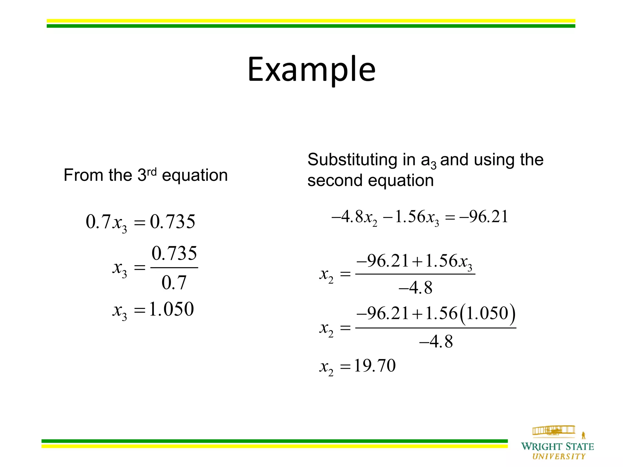
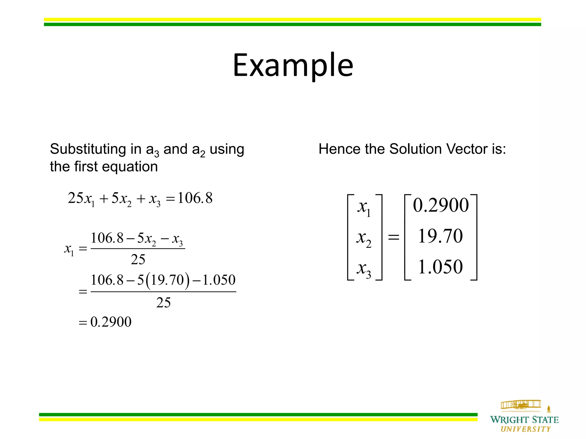
17. Example
Set [U][X] = [Z]
Solve for [X] The 3 equations become
































7350
2196
8106
7.000
56.18.40
1525
3
2
1
.
.
.
x
x
x
1 2 3
2 3
3
25 5 106.8
4.8 1.56 96.21
0.7 0.735
x x x
x x
x
  
   


18. Example
From the 3rd equation
3
3
3
0 7 0 735
0 735
0 7
1 050
. x .
.
x
.
x .



Substituting in a3 and using the
second equation
2 34 8 1 56 96 21. x . x .   
 
3
2
2
2
96 21 1 56
4 8
96 21 1 56 1 050
4 8
19 70
. . x
x
.
. . .
x
.
x .
 


 




19. Example
Substituting in a3 and a2 using
the first equation
1 2 325 5 106 8x x x .  
Hence the Solution Vector is:
1
2
3
0.2900
19.70
1.050
x
x
x
   
      
       
2 3
1
106 8 5
25
106 8 5 19 70 1 050
25
0 2900
. x x
x
. . .
.
 

 



20. Try this…
1
2
3
4
4 2 3 6 12
6 7 6.5 6 6.5
1 7.5 6.25 5.5 16
12 22 15.5 1 17
x
x
x
x
      
          
    
    
     

21. Module LU_solver
Contains
! SUBROUTINE TO PERFORM DOLITTLE FACTORIZATION: A=LU
SUBROUTINE LU(N,A,B,X)
integer::N,I,j,k
double precision:: A(N,N),L(N,N),U(N,N),B(N),Z(N),X(N)
double precision:: S,S1,S2,SS,S3,S4
DO I = 1,N
L(I,I)=1.
ENDDO
U(1,1)=A(1,1)
IF(U(1,1).EQ.0.)THEN
WRITE(1,*)'LU FACTORIZATION IS IMPOSSIBLE'
RETURN
ENDIF
DO J =2,N
U(1,J)=A(1,J) ! DETERMINE THE FIRST ROW OF U
L(J,1)=A(J,1)/U(1,1) ! DETERMINE THE FIRST COLUMN OF XL
ENDDO
DO I = 2, N-1
S=0.
DO K = 1, I-1
S=S+L(I,K)*U(K,I)
ENDDO
U(I,I)= A(I,I)-S
IF(U(I,I).EQ.0.)THEN
WRITE(1,*)'LU FACTORIZATION IS IMPOSSIBLE'
RETURN
ENDIF
DO J = I+1, N
S1=0.
S2=0.
DO K = 1, I-1
S1=S1+L(I,K)*U(K,J) ! DETERMINE THE (ith) ROWS OF U
S2=S2+L(J,K)*U(K,I) ! DETERMINE THE (ith) COLUMN OF XL
U(I,J)=A(I,J)-S1
L(J,I)=(A(J,I)-S2)/U(I,I)
ENDDO
ENDDO
ENDDO
SS=0
DO K = 1,N-1
SS=SS+L(N,K)*U(K,N)
U(N,N)=A(N,N)-SS
ENDDO
IF(U(N,N).EQ.0) THEN
WRITE(1,*)' THE MATRIX A IS SINQULAR'
ENDIF
! SUBROUTINE TO SOLVE LZ=B USING FORWARD SUBSTITUTION
Z(1)=B(1)
DO I =2,N
S3=0.
DO J =1,I-1
S3=S3+L(I,J)*Z(J)
ENDDO
Z(I)=B(I)-S3
ENDDO
X(N)=Z(N)/U(N,N)
DO K = N-1,1,-1 ! SOLVING UX=Z
S4=0.
DO J=K+1,N
S4=S4+U(K,J)*X(J)
ENDDO
X(K)=(Z(K)-S4)/U(K,K)
ENDDO
RETURN
END subroutine LU
end module solver

22. program main
use LU_solver
double precision, dimension(4,4)::A
double precision, dimension (4)::B,X
integer::i,j,N=4
open (1, file='matrix.dat')
do i=1,n
read(1,*)(a(i,j),J=1,N)
enddo
read(1,*)B
call LU(N,A,B,X)
print *,x
stop
end program main 4. -2. -3. 6.
-6. 7. 6.5 -6.
1. 7.5 6.25 5.5
-12. 22. 15.5 -1.
12. -6.5 16. 17.
matrix.dat file
1
2
3
4
4 2 3 6 12
6 7 6.5 6 6.5
1 7.5 6.25 5.5 16
12 22 15.5 1 17
x
x
x
x
      
          
    
    
     