The document covers the dynamics of polymer solutions and melts, focusing on the Rouse and Zimm models, which describe the behavior of unentangled and entangled polymers under various conditions. It emphasizes the importance of length scales, diffusion coefficients, and the effects of hydrodynamic interactions on polymer motion. Additionally, it discusses the viscoelastic properties of polymer melts and the impact of molecular weight on relaxation times and viscosities.

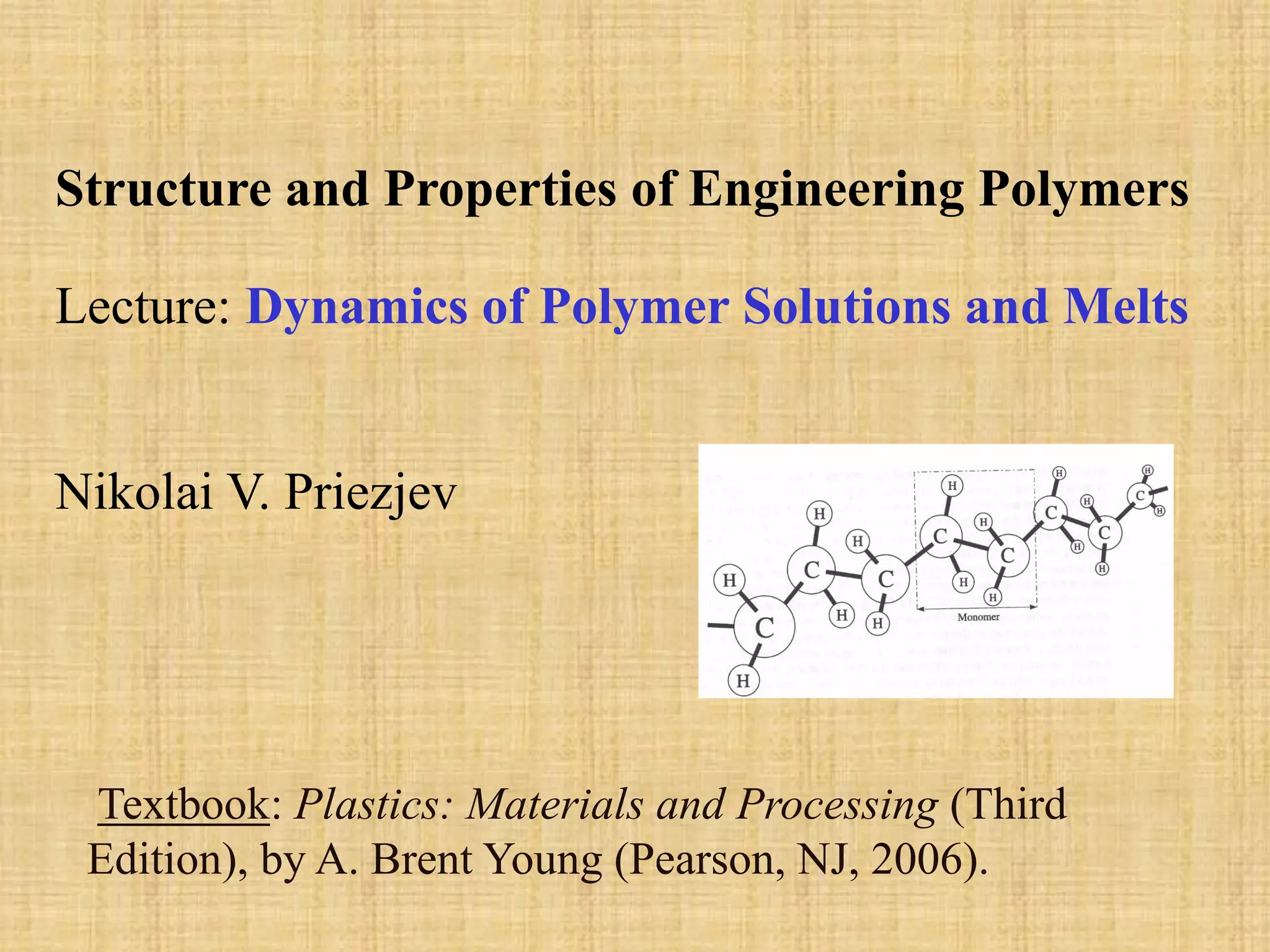
1. Textbook: Plastics: Materials and Processing (Third
Edition), by A. Brent Young (Pearson, NJ, 2006).
Structure and Properties of Engineering Polymers
Lecture: Dynamics of Polymer Solutions and Melts
Nikolai V. Priezjev

2. Dynamics of Polymer Solutions and Melts
1. Length scales and fractal structure of polymer solutions
2. Brownian diffusion of a spherical particle in a viscous fluid
3. Review of dynamics of unentangled polymer solutions (Rouse
and Zimm models)
4. Structure and dynamics of entangled polymer melts (primitive
path analysis)
M. Rubinstein & R. Colby, Polymer Physics (2003)

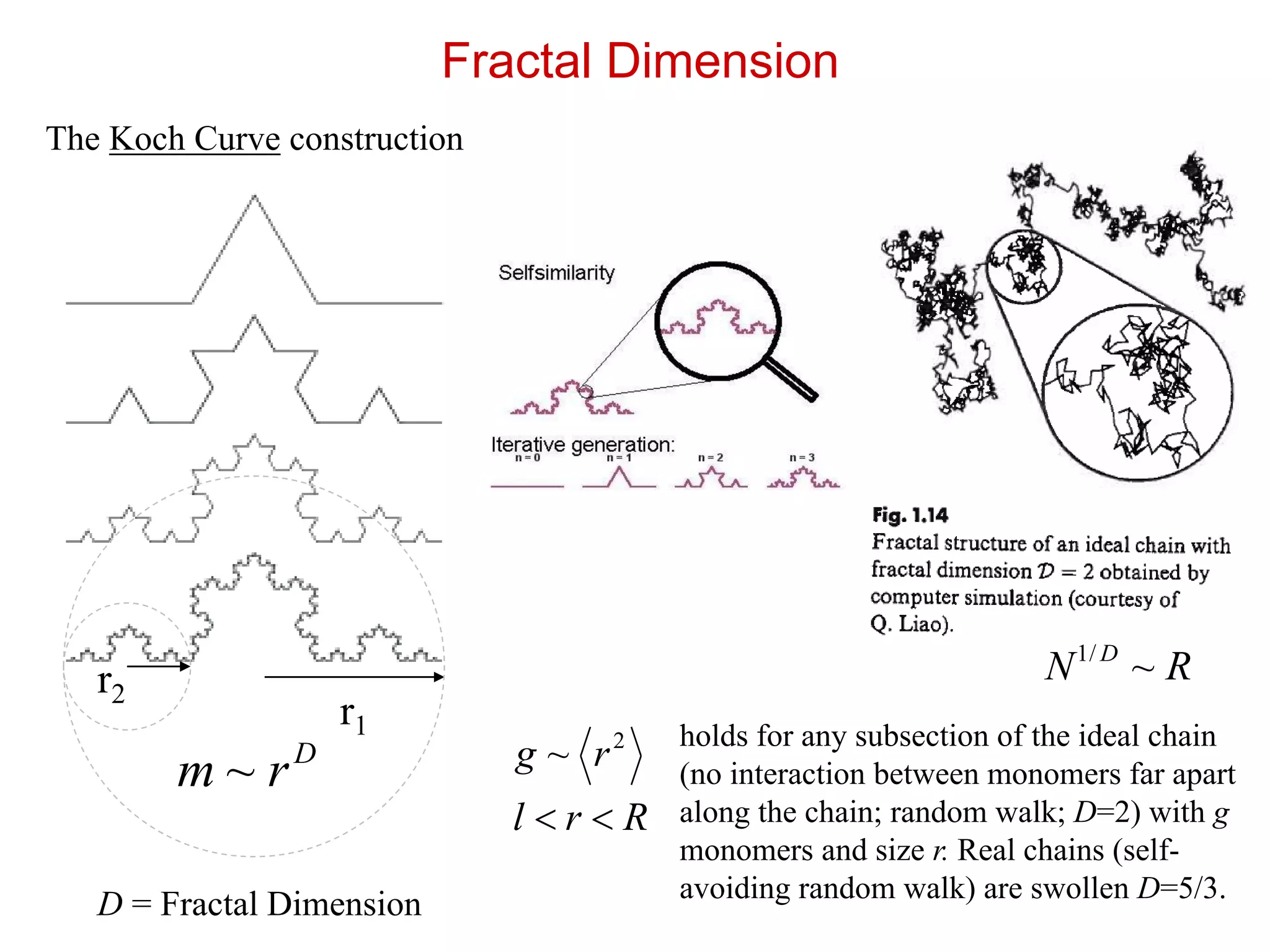
3. The Koch Curve construction
Fractal Dimension
r2
r1
D
rm ~
D = Fractal Dimension
2
~ rg
holds for any subsection of the ideal chain
(no interaction between monomers far apart
along the chain; random walk; D=2) with g
monomers and size r. Real chains (self-
avoiding random walk) are swollen D=5/3.
Rrl 
RN D
~/1

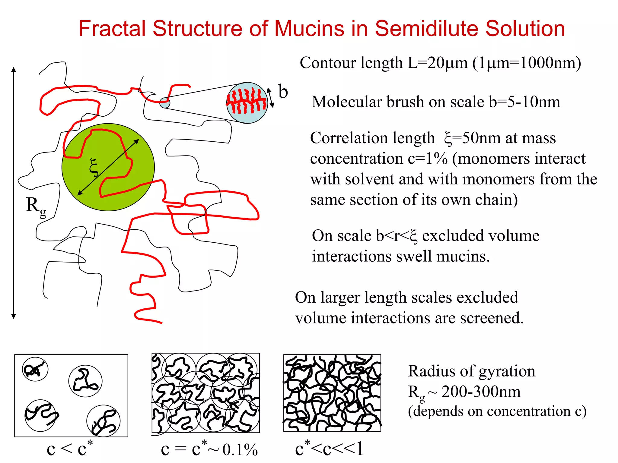
4. Fractal Structure of Mucins in Semidilute Solution
x
Correlation length x=50nm at mass
concentration c=1% (monomers interact
with solvent and with monomers from the
same section of its own chain)
b Molecular brush on scale b=5-10nm
On scale b<r<x excluded volume
interactions swell mucins.
Rg
On larger length scales excluded
volume interactions are screened.
Radius of gyration
Rg ~ 200-300nm
(depends on concentration c)
Contour length L=20mm (1mm=1000nm)
c < c* c = c*~ 0.1% c*<c<<1

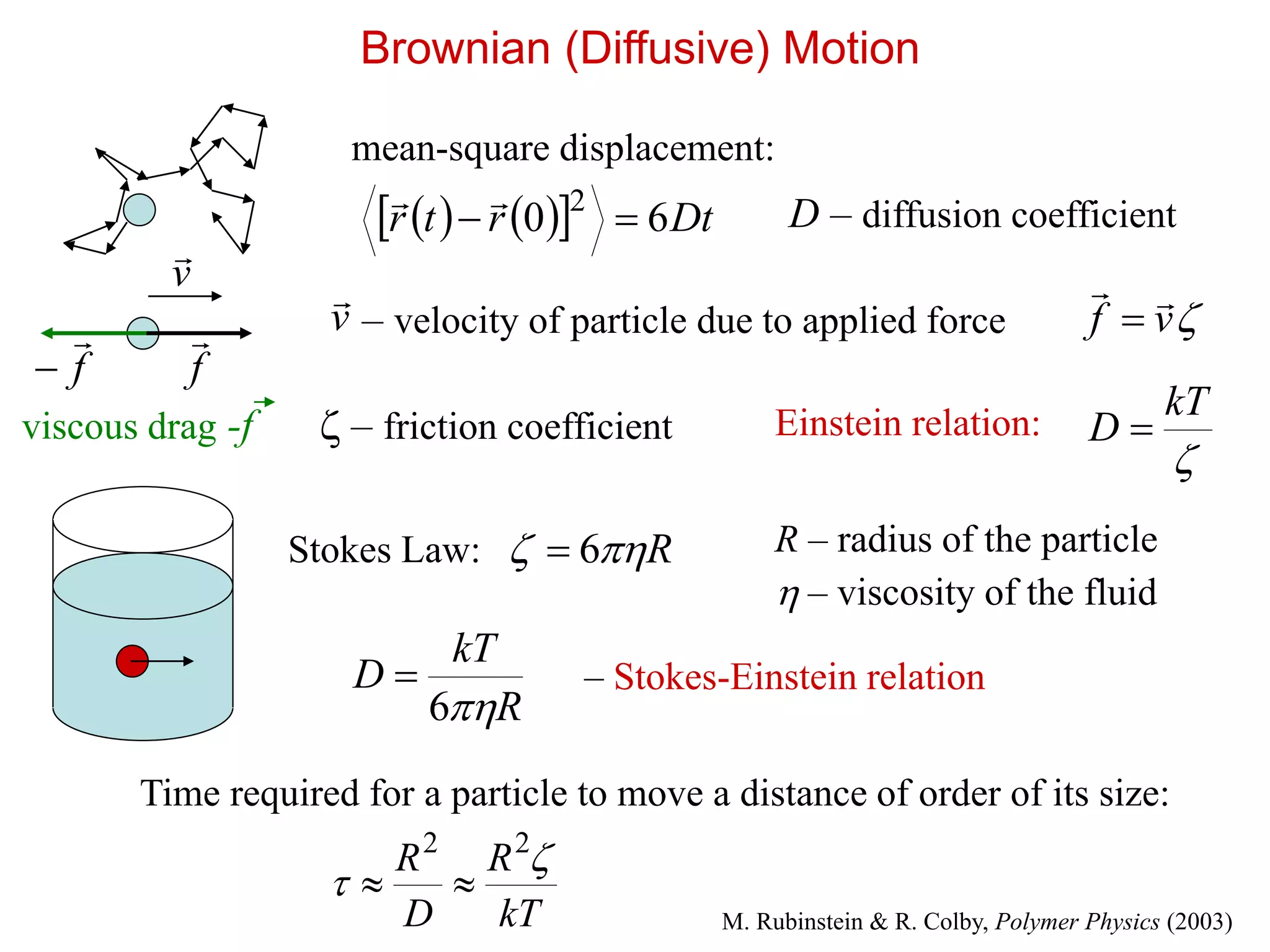
5. – velocity of particle due to applied force
Brownian (Diffusive) Motion
     Dtrtr 60 2

 D – diffusion coefficient
f

v

v

f


vf


Einstein relation:

kT
D 
Stokes Law: R 6 R – radius of the particle
 – viscosity of the fluid
R
kT
D
6
 – Stokes-Einstein relation
mean-square displacement:
viscous drag -f  – friction coefficient
kT
R
D
R 

22

Time required for a particle to move a distance of order of its size:
M. Rubinstein & R. Colby, Polymer Physics (2003)

6. N beads connected by springs
with root-mean square size b.
 – friction coefficient of a bead
R = N – total friction coefficient of the Rouse chain
 N
kTkT
DR 
R
 diffusion coefficient of the Rouse chain
2
2
NR
kTD
R
R
R

   Rouse time
for t < R – viscoelastic modes
for t > R – diffusive motion
Time required for a chain to move a distance of order of its size R
Rouse Model (1953)
Rg
M. Rubinstein & R. Colby, Polymer Physics (2003)
Ideal chain: no interaction between mono-
mers that are far apart along the chain

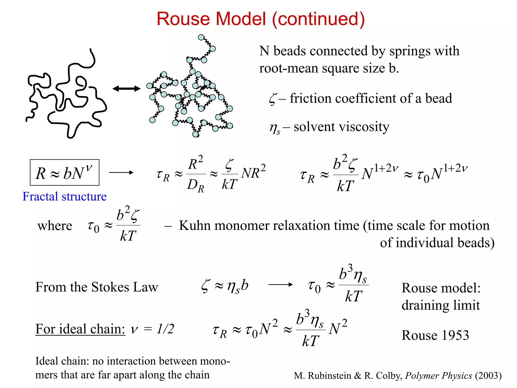
7. Rouse Model (continued)
N beads connected by springs with
root-mean square size b.
 – friction coefficient of a bead



 21
0
21
2

 NN
kT
b
R
kT
b 

2
0  – Kuhn monomer relaxation time (time scale for motion
of individual beads)
For ideal chain:  = 1/2
From the Stokes Law bs 
kT
b s

3
0 
2
3
2
0 N
kT
b
N s
R

 
Rouse model:
draining limit
2
2
NR
kTD
R
R
R

 
Fractal structure
where
Rouse 1953
s – solvent viscosity
M. Rubinstein & R. Colby, Polymer Physics (2003)

bNR 
Ideal chain: no interaction between mono-
mers that are far apart along the chain

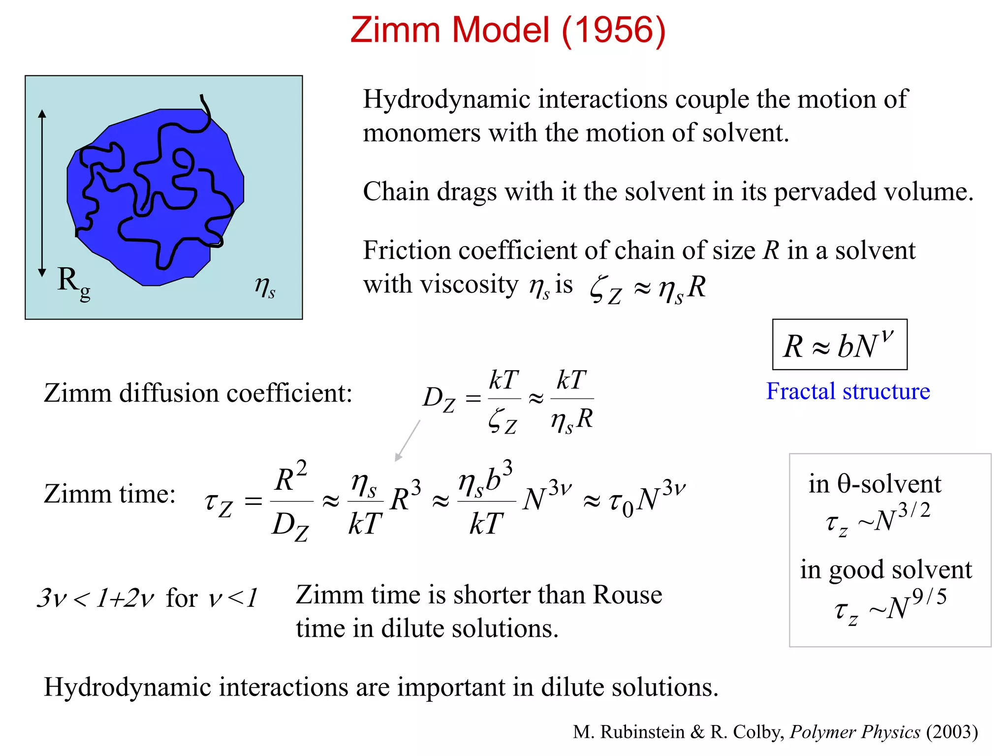
8. Zimm Model (1956)
Hydrodynamic interactions couple the motion of
monomers with the motion of solvent.
Chain drags with it the solvent in its pervaded volume.
Friction coefficient of chain of size R in a solvent
with viscosity s is RsZ  
Zimm diffusion coefficient:
R
kTkT
D
sZ
Z


Zimm time: 


 3
0
3
3
3
2
NN
kT
b
R
kTD
R ss
Z
Z 
3  12 for  <1 Zimm time is shorter than Rouse
time in dilute solutions.
Hydrodynamic interactions are important in dilute solutions.
2/3
~Nz
5/9
~Nz
in q-solvent
in good solvent

bNR 
Rg s
M. Rubinstein & R. Colby, Polymer Physics (2003)
Fractal structure

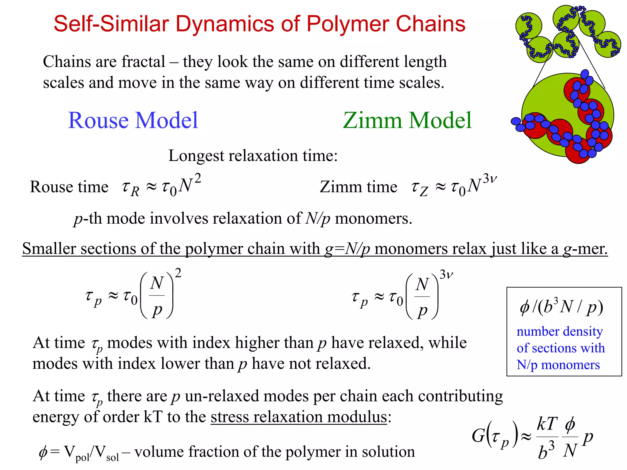
9. Self-Similar Dynamics of Polymer Chains
Rouse Model
Chains are fractal – they look the same on different length
scales and move in the same way on different time scales.
Zimm Model
Longest relaxation time:
2
0NR  Rouse time Zimm time

 3
0NZ 
Smaller sections of the polymer chain with g=N/p monomers relax just like a g-mer.
p-th mode involves relaxation of N/p monomers.
2
0 






p
N
p 


3
0 






p
N
p
At time p modes with index higher than p have relaxed, while
modes with index lower than p have not relaxed.
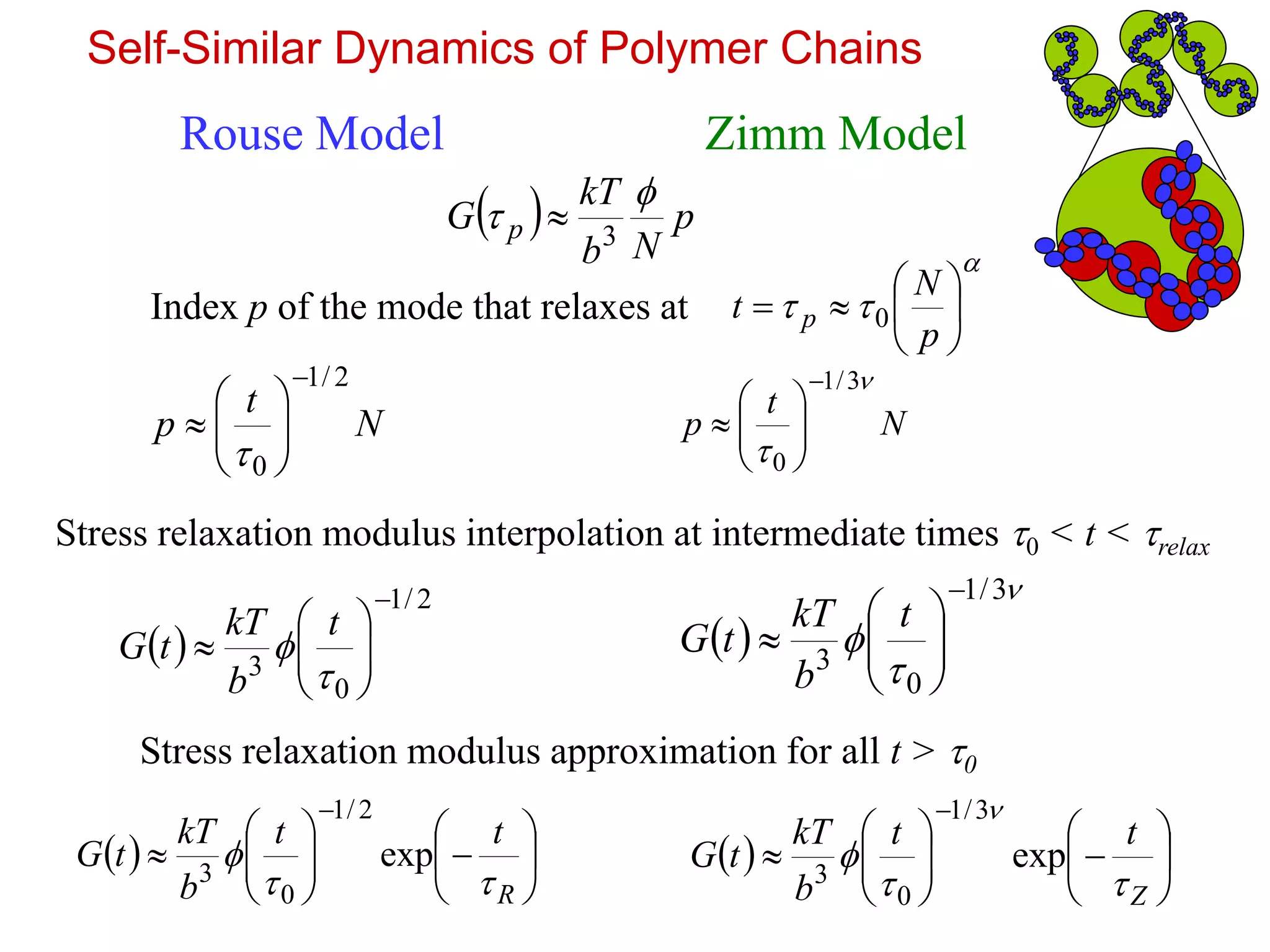
At time p there are p un-relaxed modes per chain each contributing
energy of order kT to the stress relaxation modulus:
  p
Nb
kT
G p

 3

 = Vpol/Vsol – volume fraction of the polymer in solution
)//( 3
pNb
number density
of sections with
N/p monomers

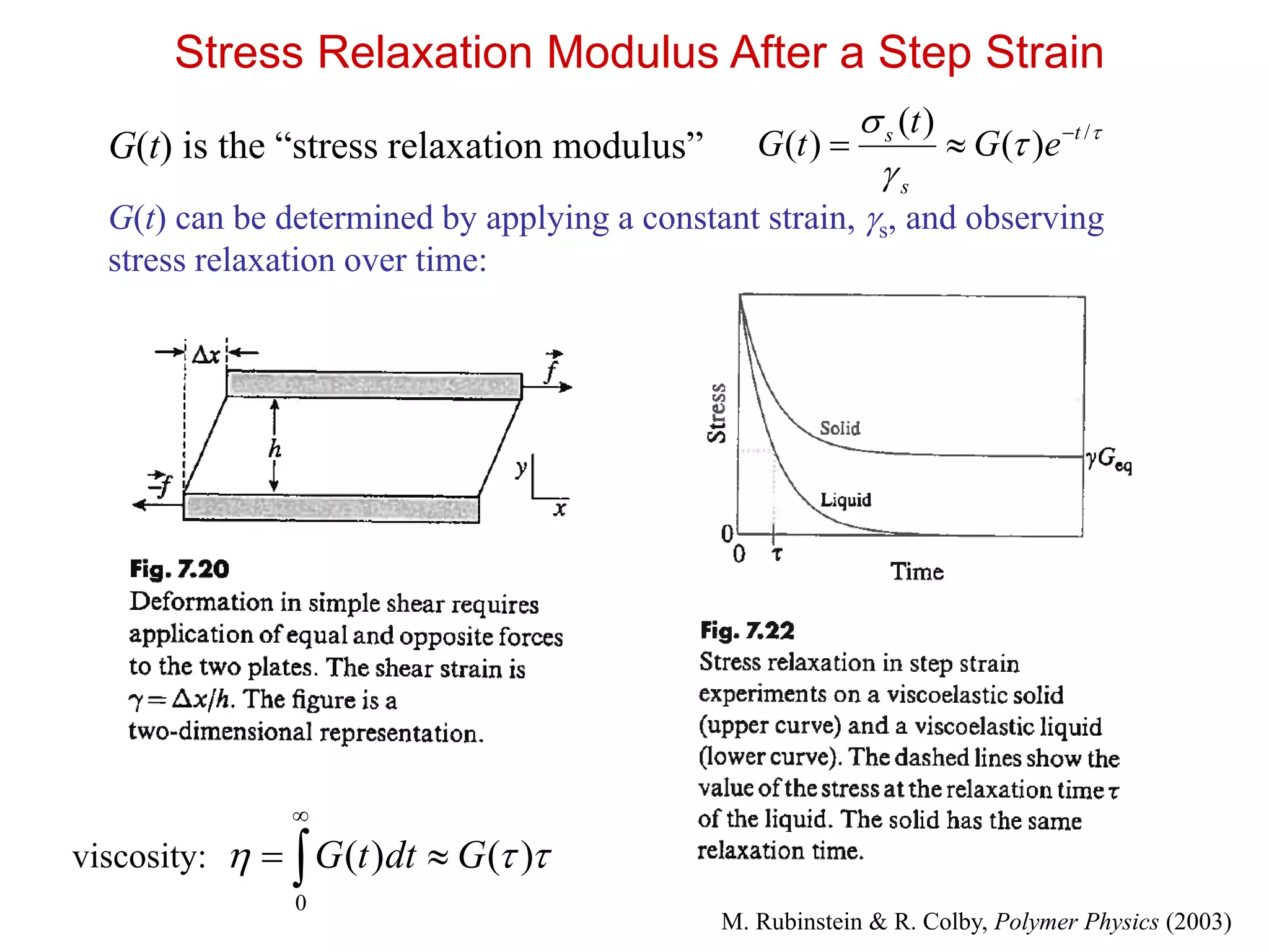
10. Stress Relaxation Modulus After a Step Strain
G(t) is the “stress relaxation modulus”
G(t) can be determined by applying a constant strain, s, and observing
stress relaxation over time:



 /
)(
)(
)( t
s
s
eG
t
tG 

 )()(
0
GdttG  

viscosity:
M. Rubinstein & R. Colby, Polymer Physics (2003)

11.   p
Nb
kT
G p

 3

Index p of the mode that relaxes at
N
t
p
2/1
0









Stress relaxation modulus interpolation at intermediate times 0 < t < relax
 
2/1
0
3










t
b
kT
tG
N
t
p


3/1
0









 






p
N
t p 0
 



3/1
0
3








t
b
kT
tG
  













R
tt
b
kT
tG

 exp
2/1
0
3
  













Z
tt
b
kT
tG



exp
3/1
0
3
Stress relaxation modulus approximation for all t > 0
Rouse Model Zimm Model
Self-Similar Dynamics of Polymer Chains

12. t/0
100 101 102 103 104 105 106 107
b
3
G(t)/kT
10-8
10-7
10-6
10-5
10-4
10-3
10-2
10-1
100
-1/2
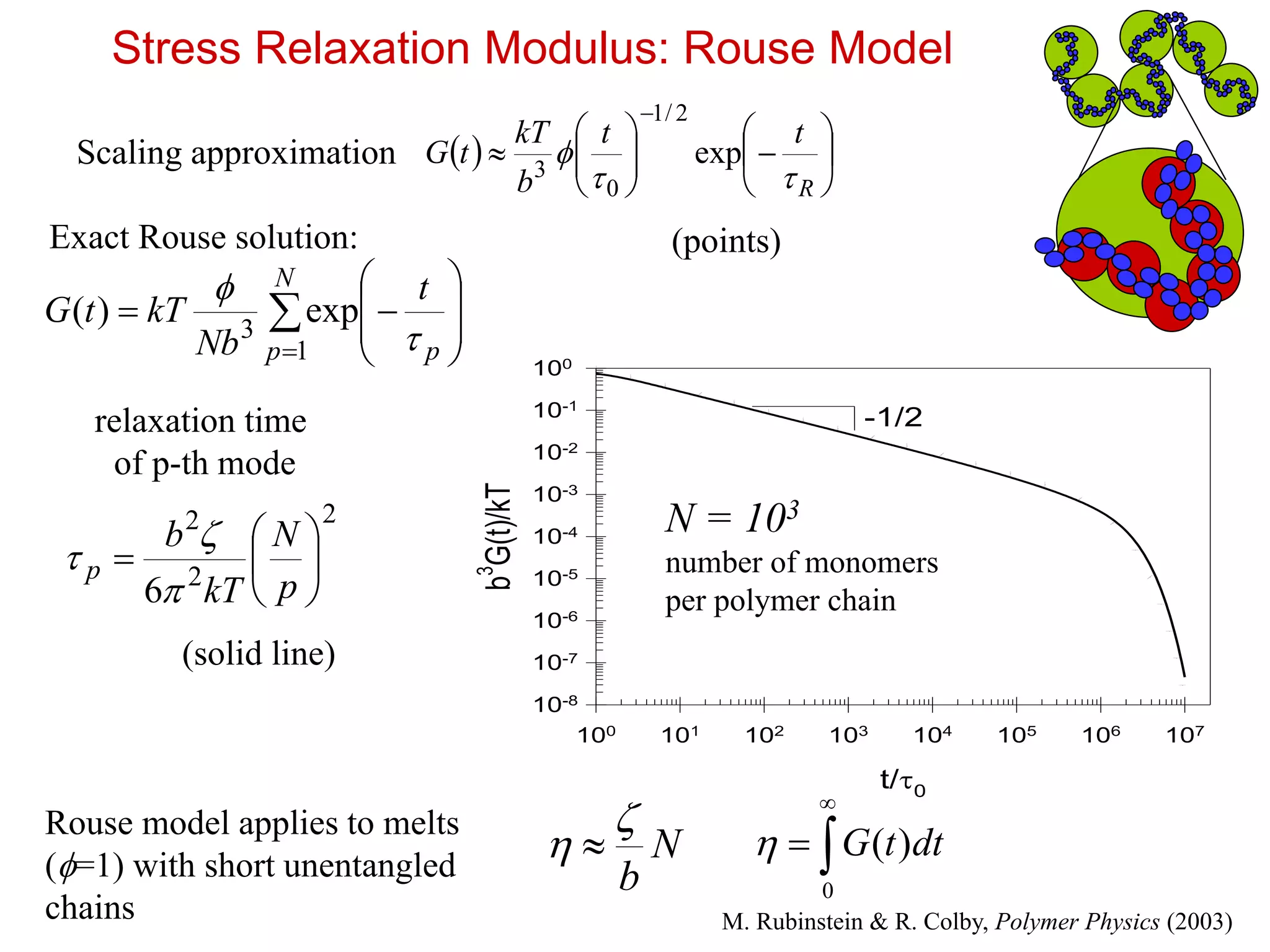
Stress Relaxation Modulus: Rouse Model
  













R
tt
b
kT
tG

 exp
2/1
0
3
Scaling approximation
relaxation time
of p-th mode











N
p p
t
Nb
kTtG
1
3
exp)(


2
2
2
6







p
N
kT
b
p



Exact Rouse solution: (points)
(solid line)
N = 103
number of monomers
per polymer chain
Rouse model applies to melts
(=1) with short unentangled
chains
N
b

  


0
)( dttG
M. Rubinstein & R. Colby, Polymer Physics (2003)

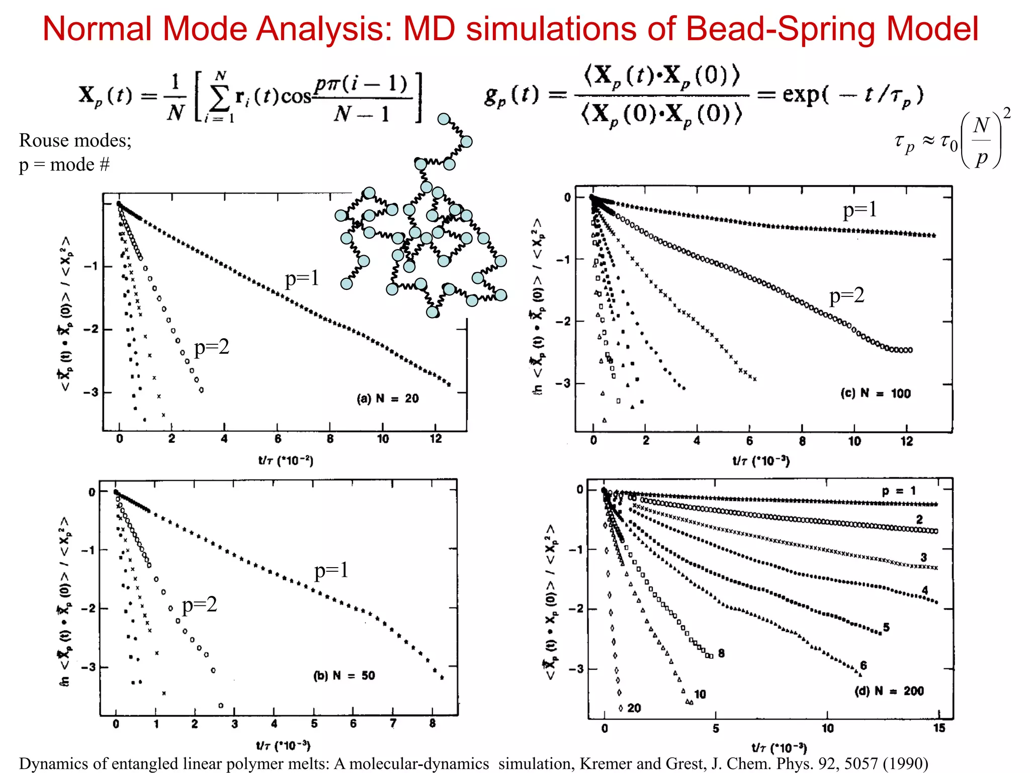
13. Normal Mode Analysis: MD simulations of Bead-Spring Model
Dynamics of entangled linear polymer melts: A molecular-dynamics simulation, Kremer and Grest, J. Chem. Phys. 92, 5057 (1990)
Rouse modes;
p = mode #
2
0 






p
N
p 
p=1
p=1
p=1
p=2
p=2
p=2

14. Mean Square Displacement of Monomers
Rouse Model
Section of N/p monomers moves by its size b(N/p)1/2 during its relaxation time p
    


2
22
0 






p
N
brr jpj

       2/1
0
22
/0 tbrtr jj 

Mean square monomer displacement for 0 < t < relax
Zimm Model
for ideal chain  = 1/2
       3/2
0
22
/0 tbrtr jj 

p/N = (t/t0)-1/2 p/N = (t/t0)-1/3
Sub-diffusive motion
    2
0jj rtr


t
0
b2
1/2
1
R
R2
1
2/3
Sections of N/p monomers move coherently
on time scale p
Z
Monomer motion in Zimm model is faster
than in Rouse model
ok for melts ok for dilute solutions
     Dtrtr 60 2



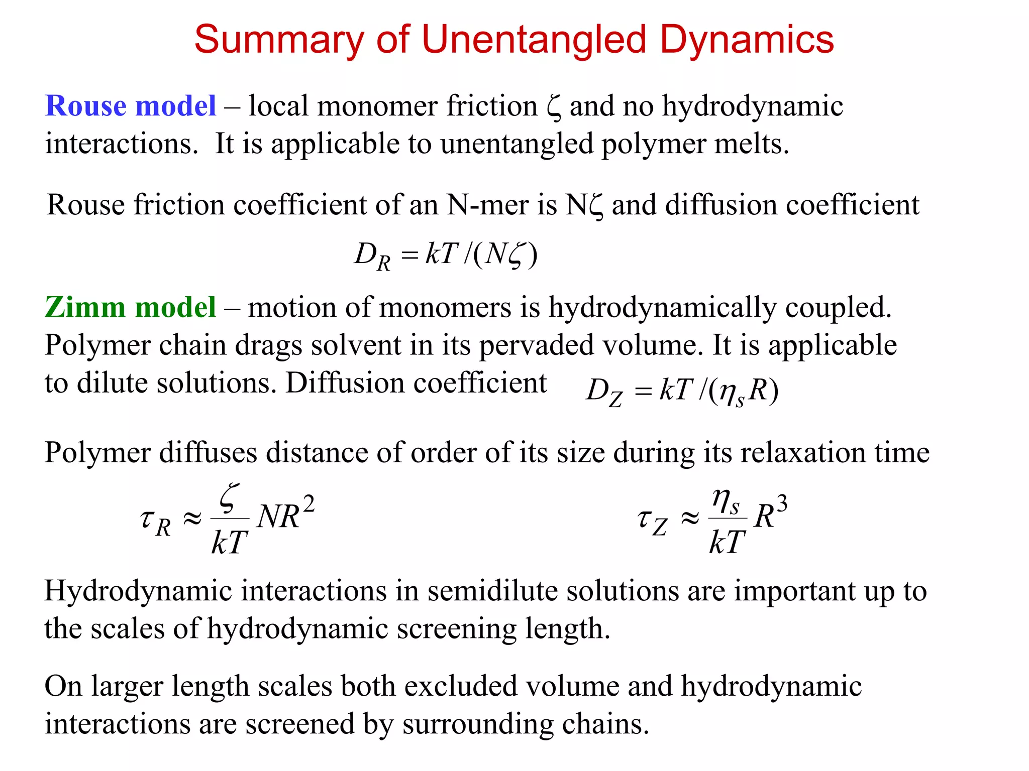
15. Summary of Unentangled Dynamics
Rouse model – local monomer friction  and no hydrodynamic
interactions. It is applicable to unentangled polymer melts.
Rouse friction coefficient of an N-mer is N and diffusion coefficient
)/( NkTDR 
Zimm model – motion of monomers is hydrodynamically coupled.
Polymer chain drags solvent in its pervaded volume. It is applicable
to dilute solutions. Diffusion coefficient )/( RkTD sZ 
Polymer diffuses distance of order of its size during its relaxation time
2
NR
kT
R

  3
R
kT
s
Z

 
Hydrodynamic interactions in semidilute solutions are important up to
the scales of hydrodynamic screening length.
On larger length scales both excluded volume and hydrodynamic
interactions are screened by surrounding chains.

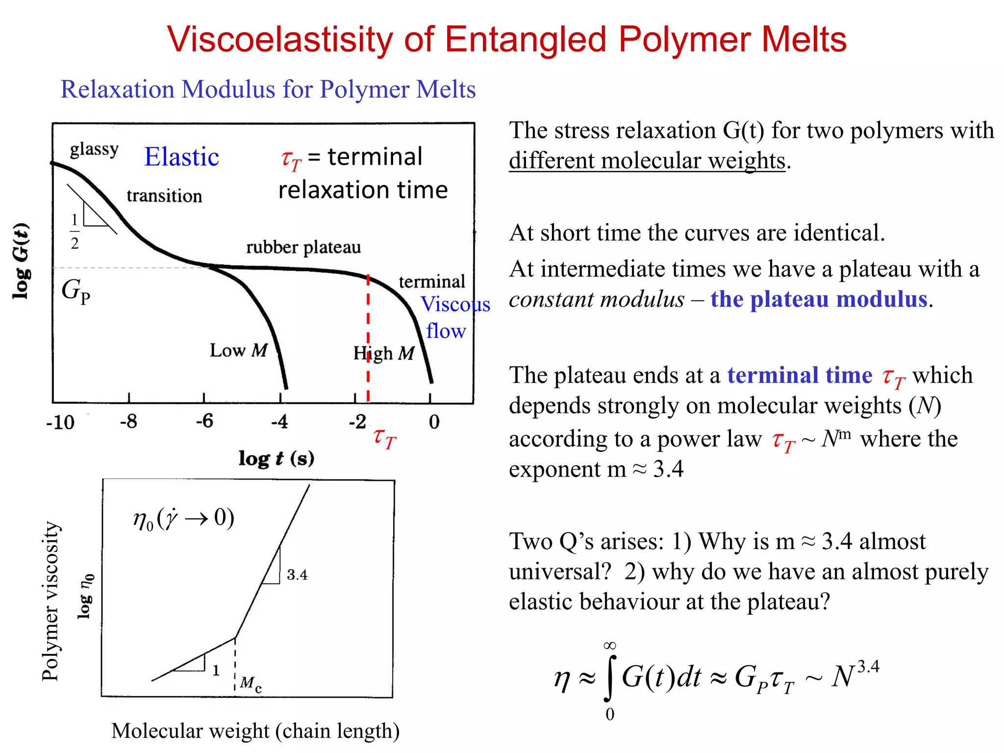
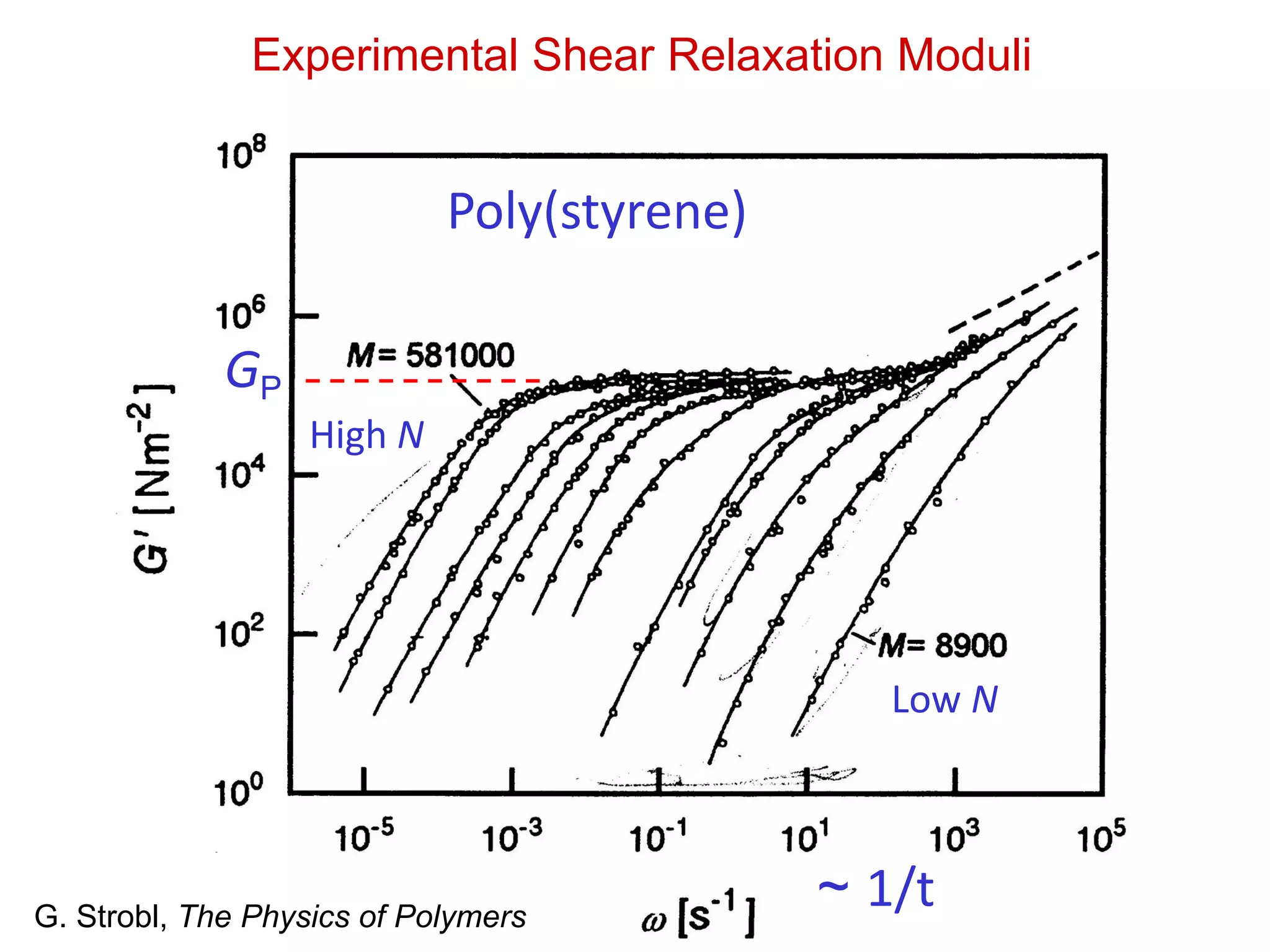
16. Viscoelastisity of Entangled Polymer Melts
T
Elastic T = terminal
relaxation time
Viscous
flow
Relaxation Modulus for Polymer Melts
The stress relaxation G(t) for two polymers with
different molecular weights.
At short time the curves are identical.
At intermediate times we have a plateau with a
constant modulus – the plateau modulus.
The plateau ends at a terminal time T which
depends strongly on molecular weights (N)
according to a power law T ~ Nm where the
exponent m ≈ 3.4
Two Q’s arises: 1) Why is m ≈ 3.4 almost
universal? 2) why do we have an almost purely
elastic behaviour at the plateau?
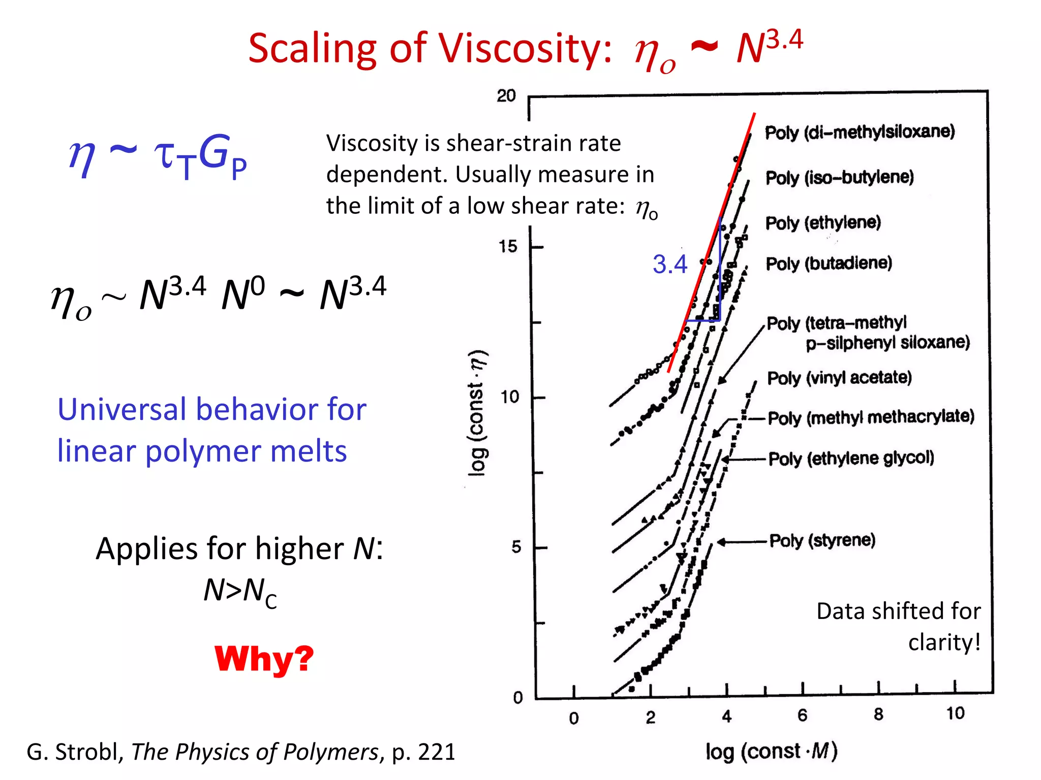
Polymerviscosity
Molecular weight (chain length)
2
1
GP
4.3
0
~)( NGdttG TP  

)0(0  

17. Experimental Shear Relaxation Moduli
Poly(styrene)
GP
Low N
High N
~ 1/tG. Strobl, The Physics of Polymers

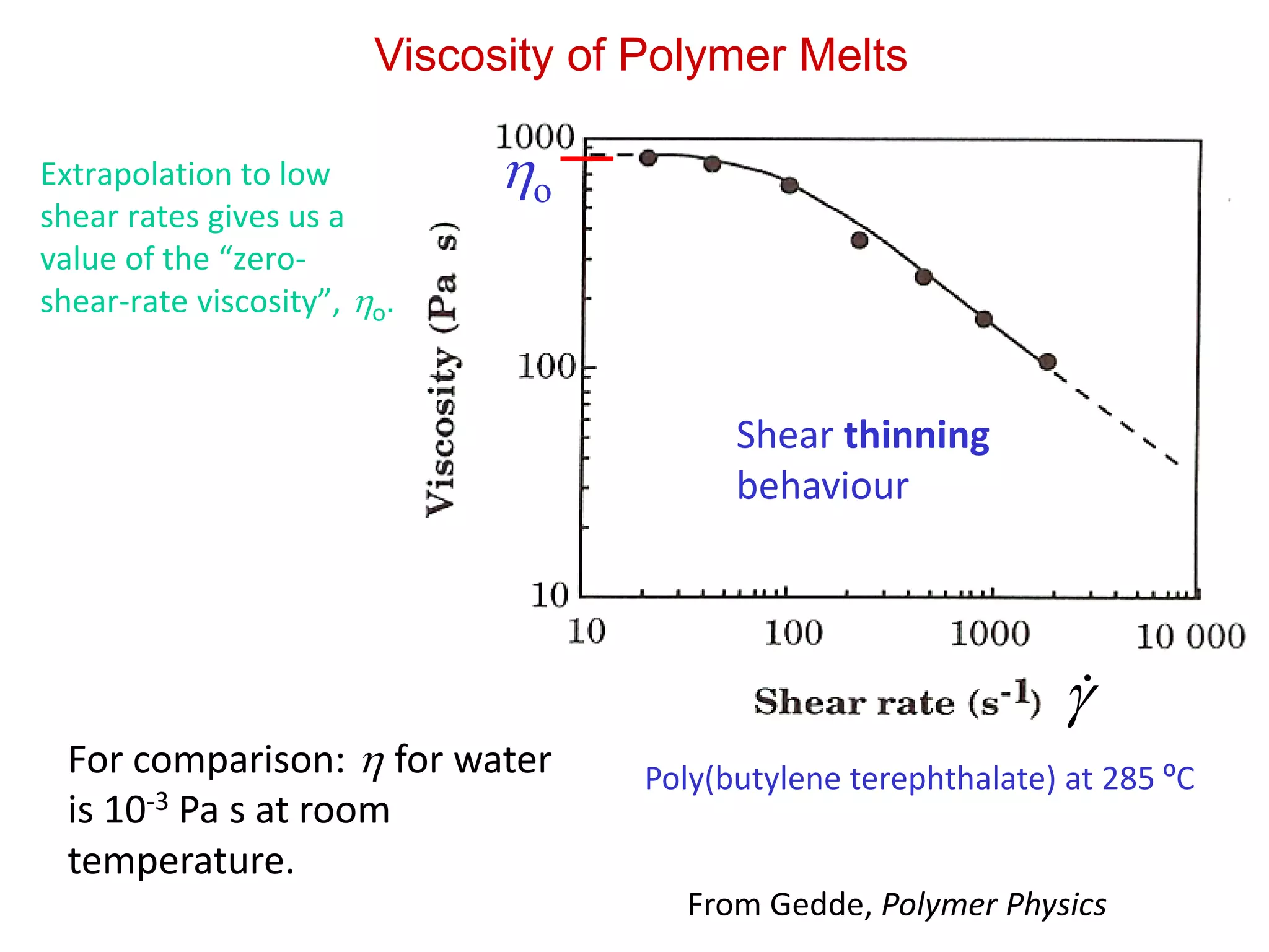
18. Viscosity of Polymer Melts
Poly(butylene terephthalate) at 285 ºCFor comparison:  for water
is 10-3 Pa s at room
temperature.
Shear thinning
behaviour
Extrapolation to low
shear rates gives us a
value of the “zero-
shear-rate viscosity”, o.

o
From Gedde, Polymer Physics

19.  ~ TGP
o ~ N3.4 N0 ~ N3.4
Universal behavior for
linear polymer melts
Applies for higher N:
N>NC
Why?
G. Strobl, The Physics of Polymers, p. 221
Data shifted for
clarity!
Viscosity is shear-strain rate
dependent. Usually measure in
the limit of a low shear rate: o
3.4
Scaling of Viscosity: o ~ N3.4

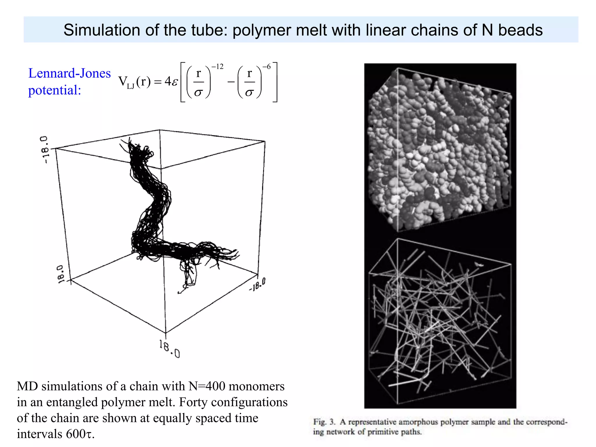
20. FENE bead-
spring model:
2
2
FENE o 2
o
1 r
V (r) kr ln 1
2 r
 
  
 
k = 30 2 and ro = 1.5
Lennard-Jones
potential:
12 6
LJ
r r
V (r) 4
 
 
    
     
     
Simulation of the tube: polymer melt with linear chains of N beads
MD simulations of a chain with N=400 monomers
in an entangled polymer melt. Forty configurations
of the chain are shown at equally spaced time
intervals 600.

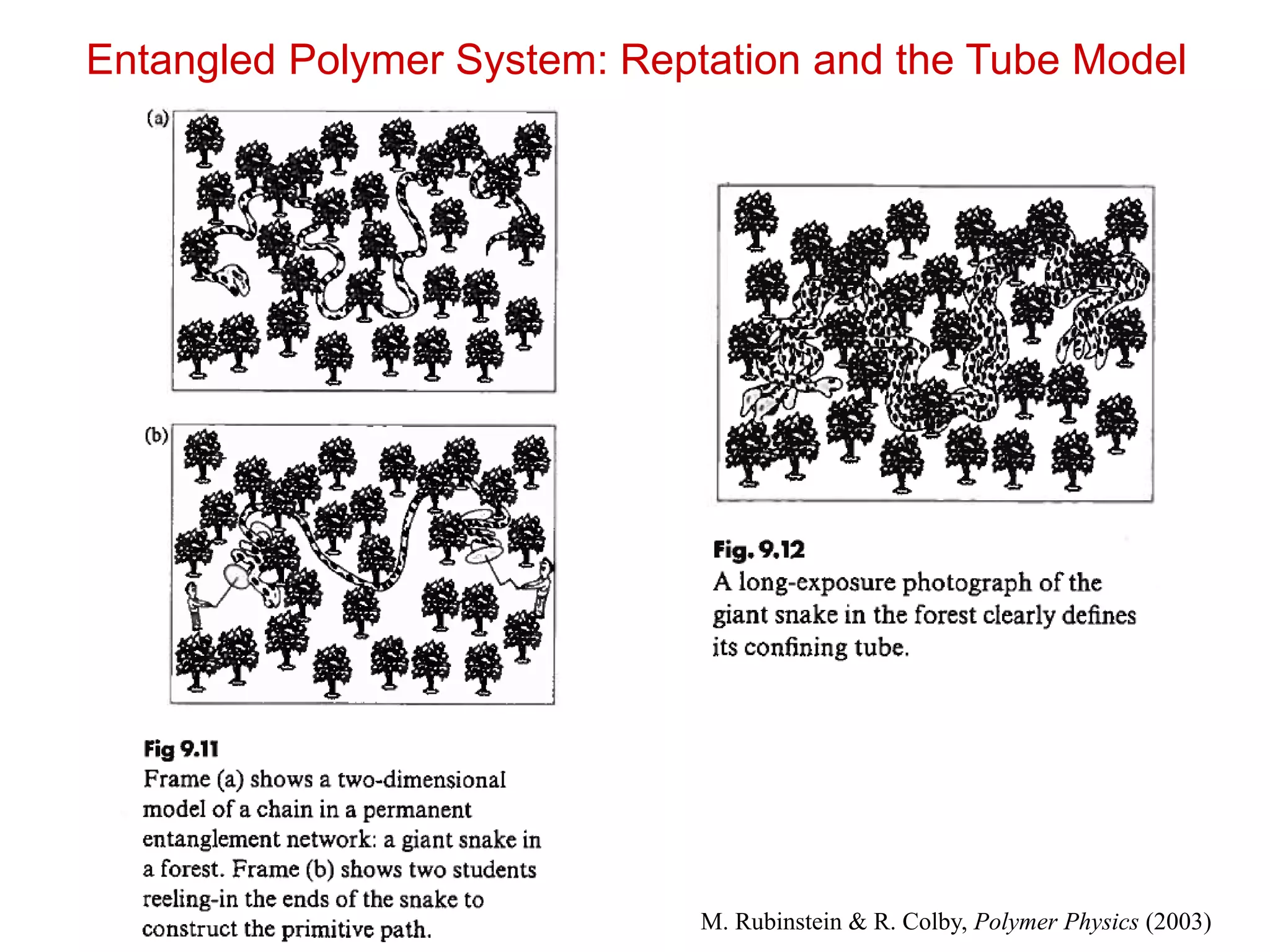
21. Entangled Polymer System: Reptation and the Tube Model
M. Rubinstein & R. Colby, Polymer Physics (2003)

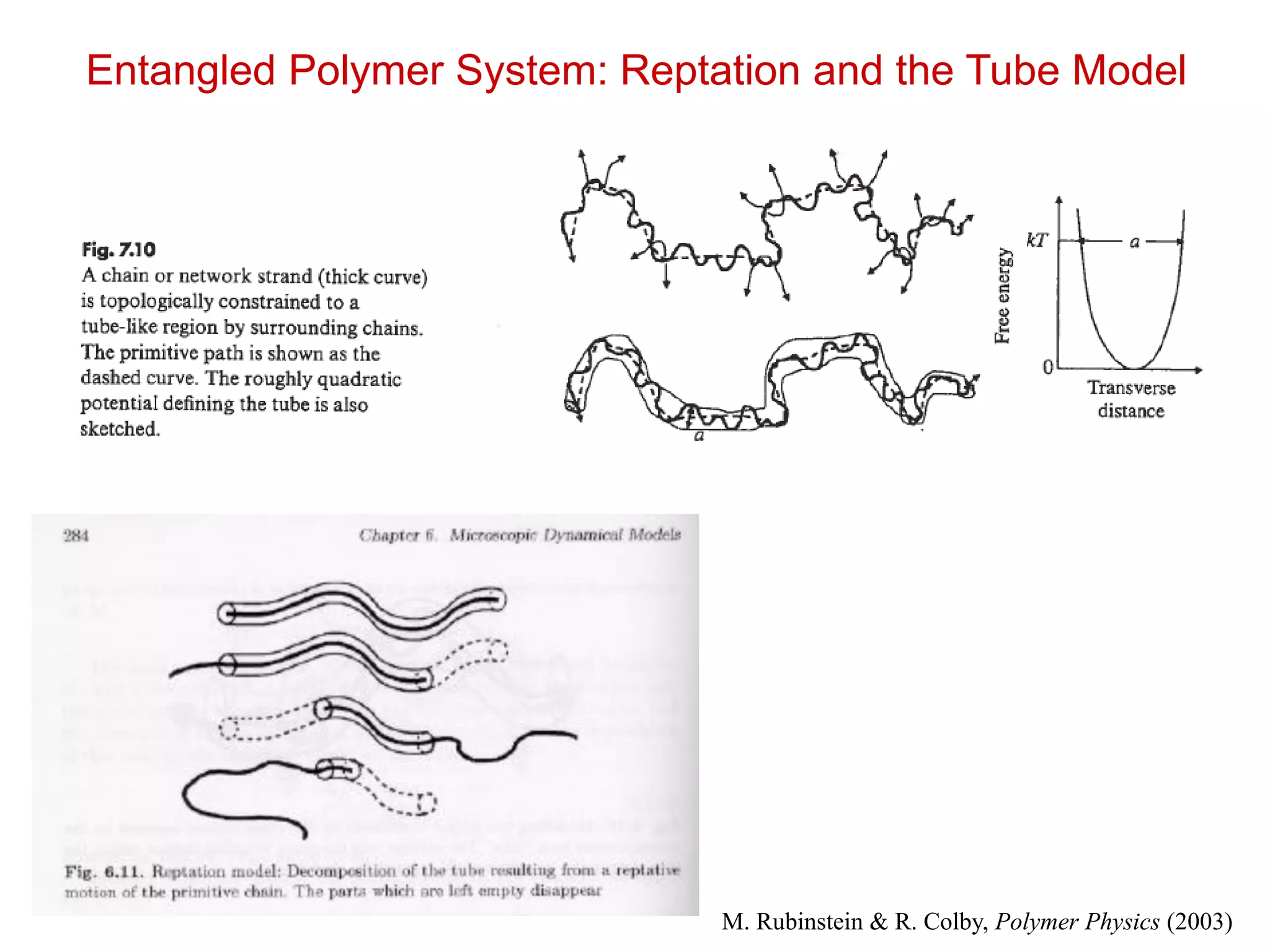
22. Entangled Polymer System: Reptation and the Tube Model
M. Rubinstein & R. Colby, Polymer Physics (2003)

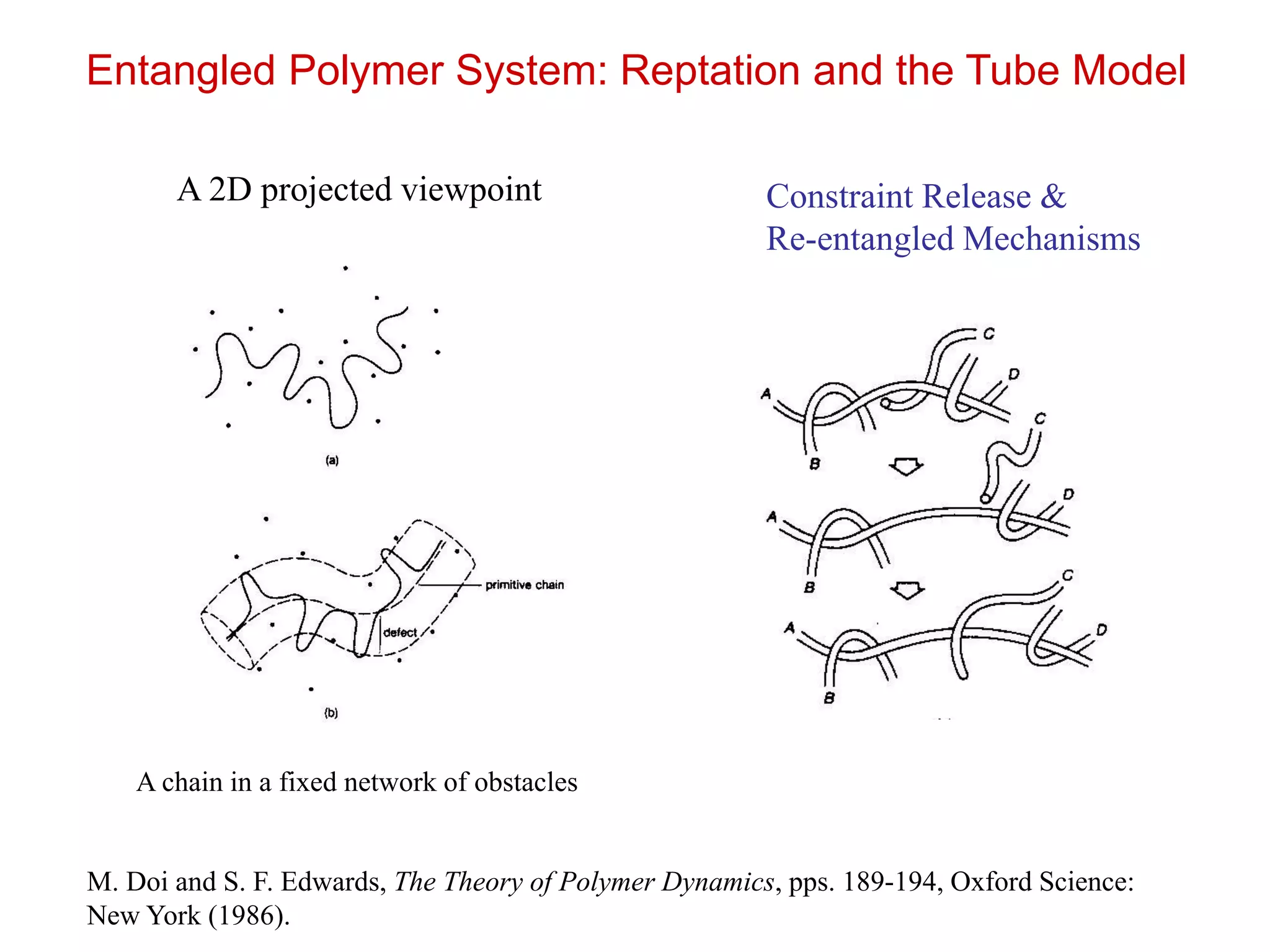
23. Entangled Polymer System: Reptation and the Tube Model
M. Doi and S. F. Edwards, The Theory of Polymer Dynamics, pps. 189-194, Oxford Science:
New York (1986).
Constraint Release &
Re-entangled Mechanisms
A 2D projected viewpoint
A chain in a fixed network of obstacles

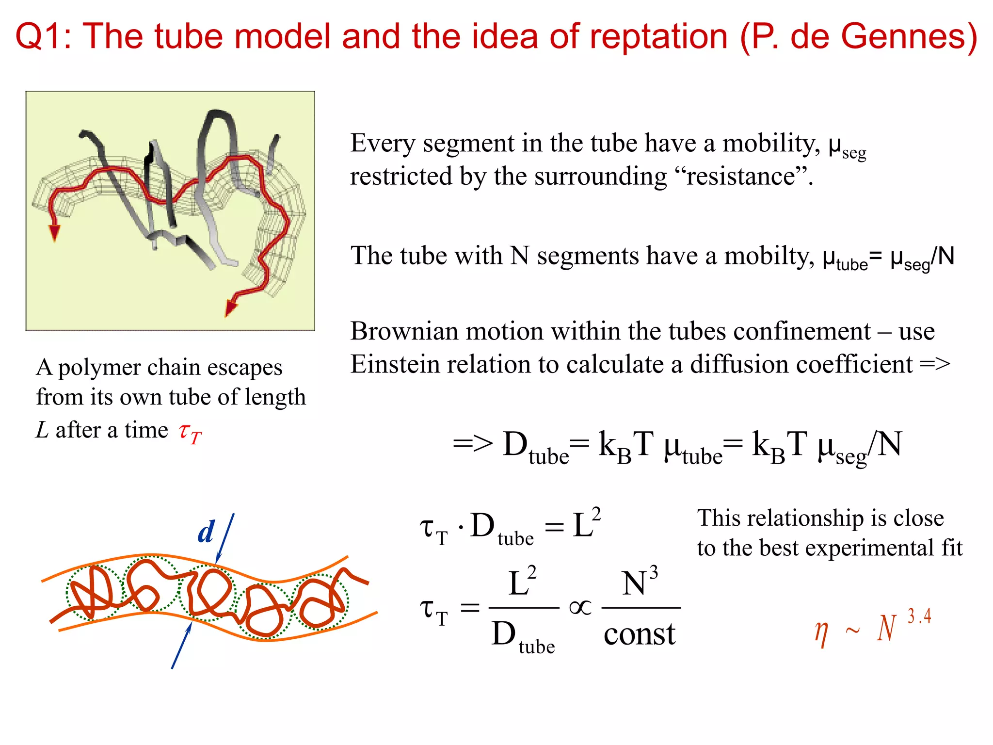
24. Q1: The tube model and the idea of reptation (P. de Gennes)
Every segment in the tube have a mobility, μseg
restricted by the surrounding “resistance”.
The tube with N segments have a mobilty, μtube= μseg/N
Brownian motion within the tubes confinement – use
Einstein relation to calculate a diffusion coefficient =>
=> Dtube= kBT μtube= kBT μseg/N
A polymer chain escapes
from its own tube of length
L after a time T
const
N
D
L
LD
3
tube
2
T
2
tubeT

d This relationship is close
to the best experimental fit
4.3
~ N

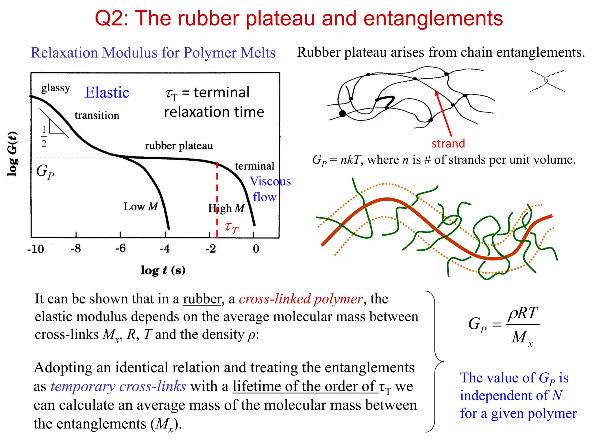
25. Q2: The rubber plateau and entanglements
T
Elastic T = terminal
relaxation time
Viscous
flow
Relaxation Modulus for Polymer Melts
2
1
GP
Rubber plateau arises from chain entanglements.
It can be shown that in a rubber, a cross-linked polymer, the
elastic modulus depends on the average molecular mass between
cross-links Mx, R, T and the density ρ:
x
P
M
RT
G


Adopting an identical relation and treating the entanglements
as temporary cross-links with a lifetime of the order of τT we
can calculate an average mass of the molecular mass between
the entanglements (Mx).

strand
The value of GP is
independent of N
for a given polymer
GP = nkT, where n is # of strands per unit volume.

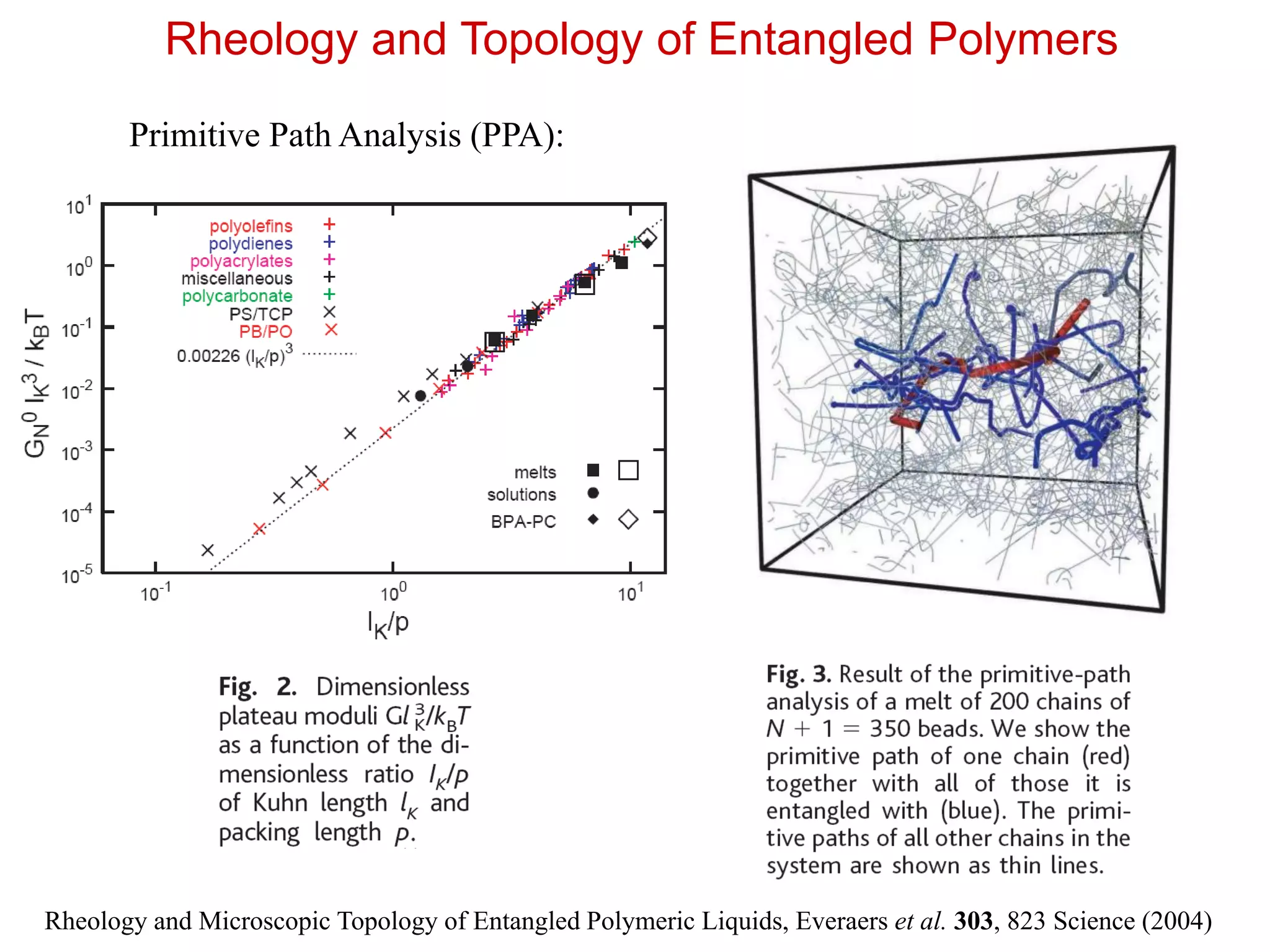
26. Rheology and Topology of Entangled Polymers
Rheology and Microscopic Topology of Entangled Polymeric Liquids, Everaers et al. 303, 823 Science (2004)
Primitive Path Analysis (PPA):

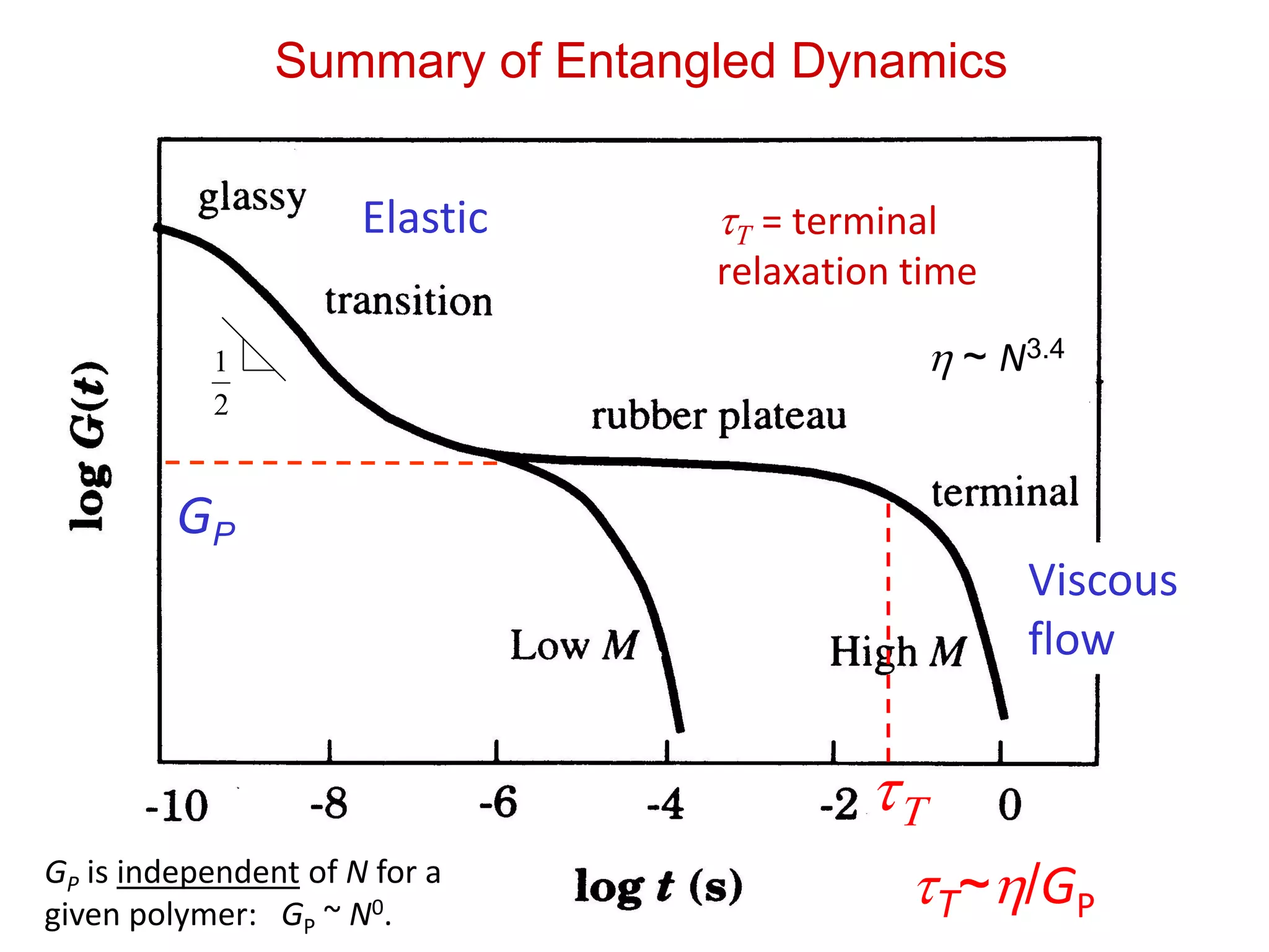
27. Summary of Entangled Dynamics
Viscous
flow
T
Elastic T = terminal
relaxation time
2
1
GP
GP is independent of N for a
given polymer: GP ~ N0.
T~/GP
 ~ N3.4

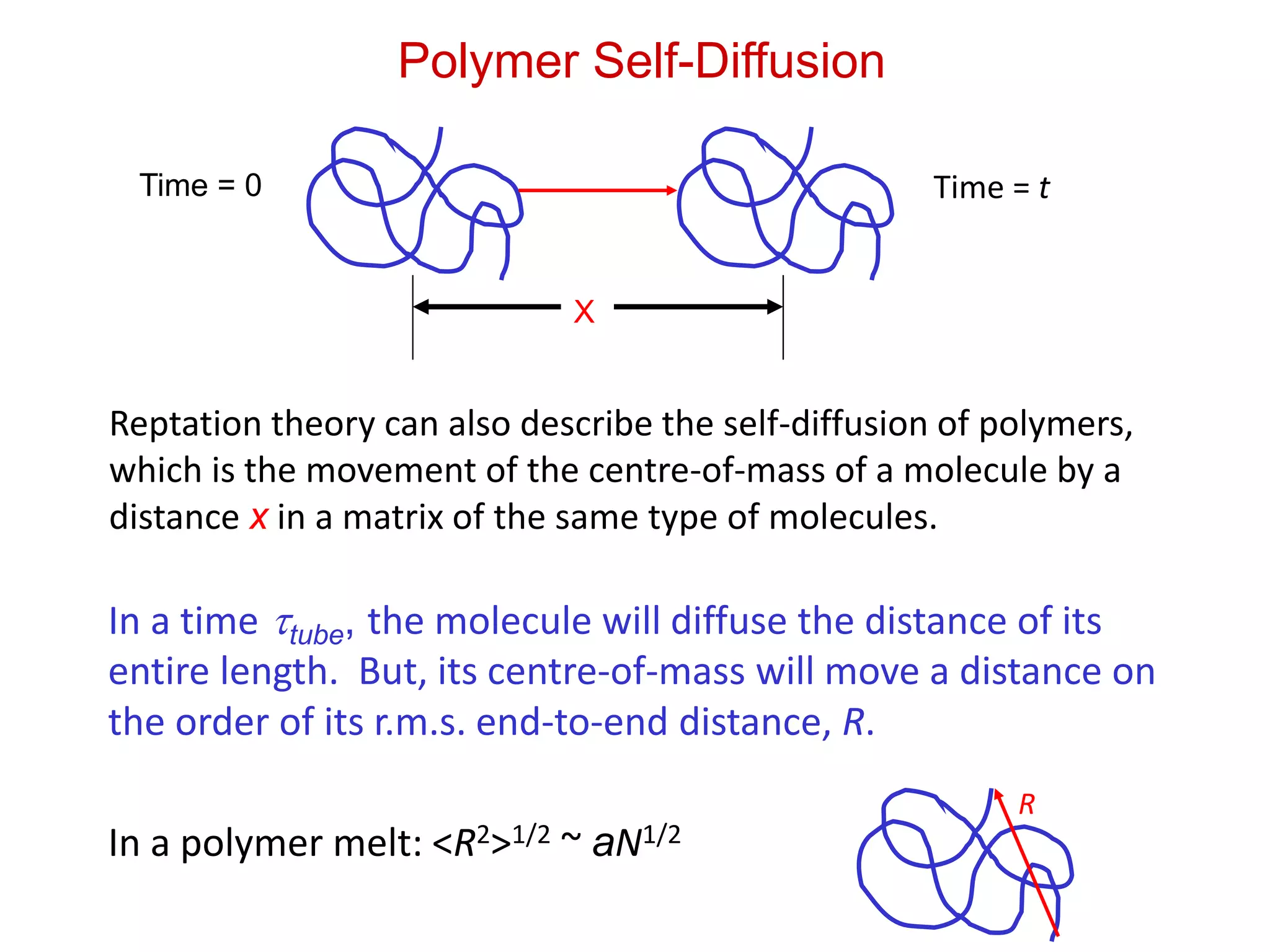
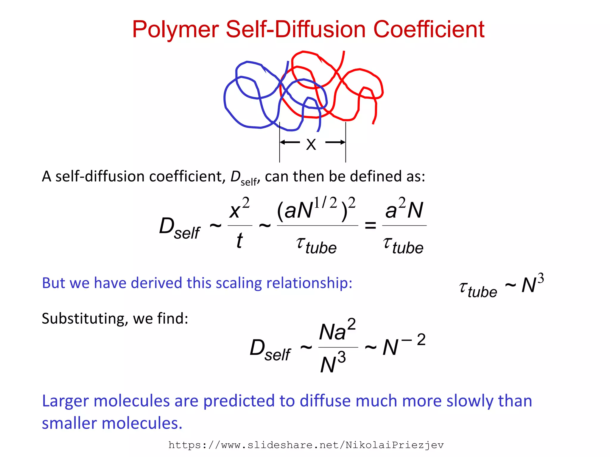
28. Polymer Self-Diffusion
X
Time = 0 Time = t
Reptation theory can also describe the self-diffusion of polymers,
which is the movement of the centre-of-mass of a molecule by a
distance x in a matrix of the same type of molecules.
In a time tube, the molecule will diffuse the distance of its
entire length. But, its centre-of-mass will move a distance on
the order of its r.m.s. end-to-end distance, R.
In a polymer melt: <R2>1/2 ~ aN1/2
R

29. Polymer Self-Diffusion Coefficient
X
tubetube
self
NaaN
t
x
D

22212
=
)(
~~
/
A self-diffusion coefficient, Dself, can then be defined as:
Larger molecules are predicted to diffuse much more slowly than
smaller molecules.
But we have derived this scaling relationship: 3
Ntube ~
Substituting, we find:
2
3
2
~~ N
N
Na
Dself
https://www.slideshare.net/NikolaiPriezjev

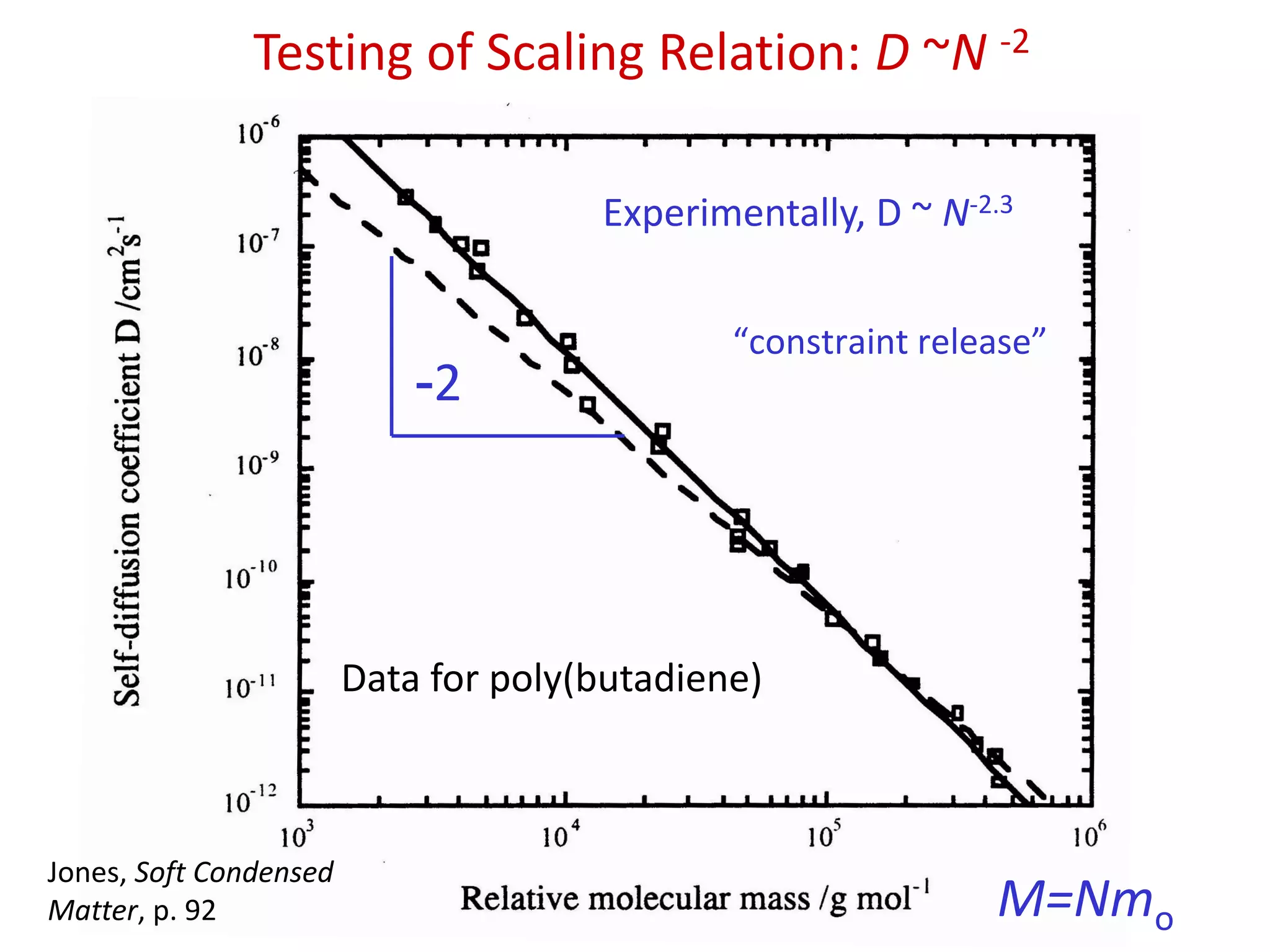
30. Testing of Scaling Relation: D ~N -2
M=Nmo
-2
Experimentally, D ~ N-2.3
Data for poly(butadiene)
Jones, Soft Condensed
Matter, p. 92
“constraint release”

31. Application of Theory: Electrophoresis

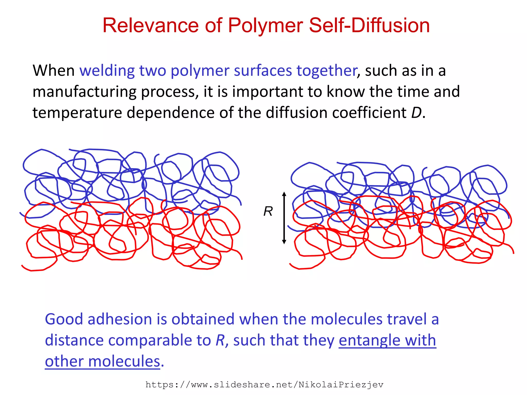
32. Relevance of Polymer Self-Diffusion
When welding two polymer surfaces together, such as in a
manufacturing process, it is important to know the time and
temperature dependence of the diffusion coefficient D.
Good adhesion is obtained when the molecules travel a
distance comparable to R, such that they entangle with
other molecules.
R
https://www.slideshare.net/NikolaiPriezjev

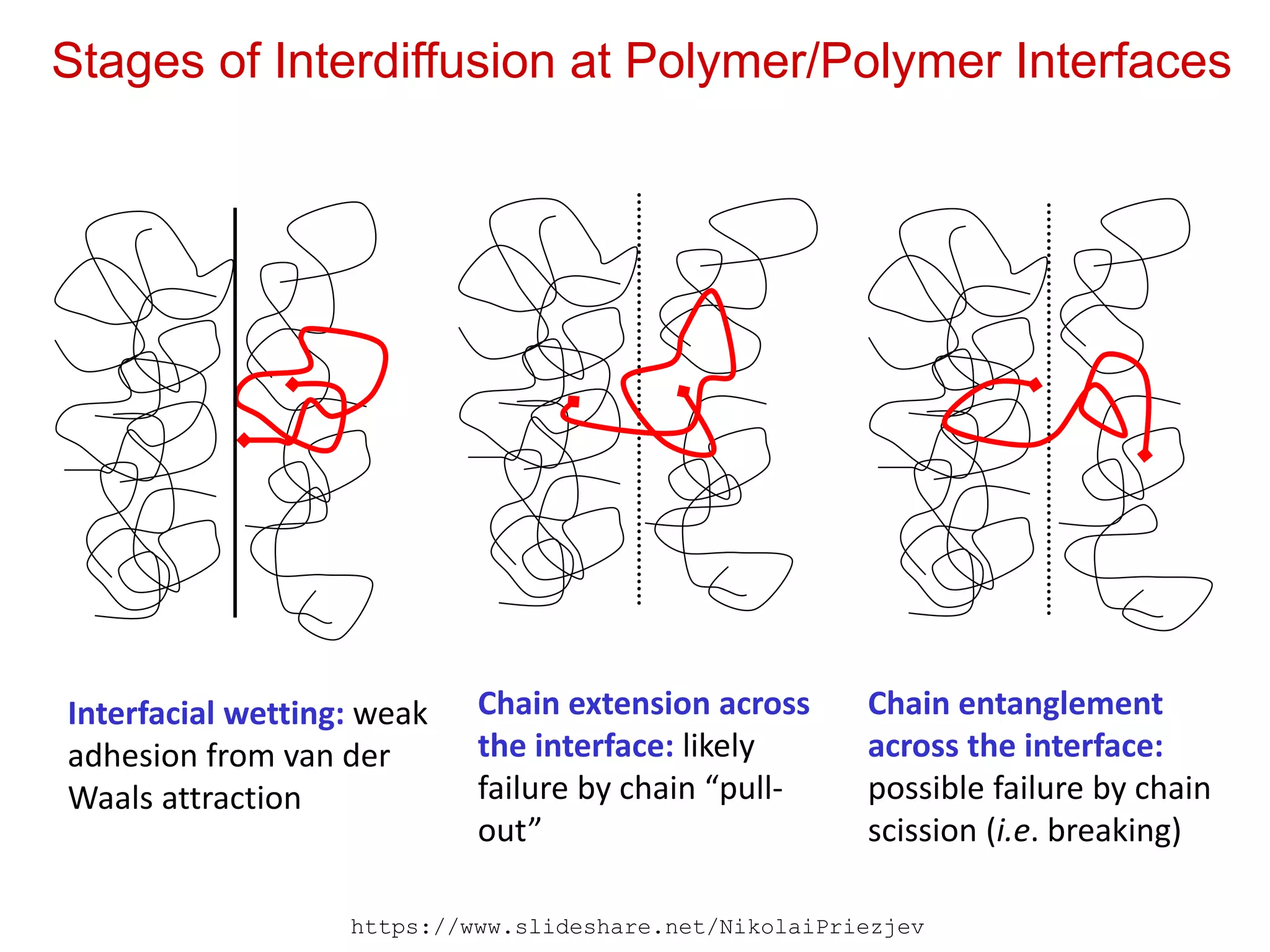
33. Stages of Interdiffusion at Polymer/Polymer Interfaces
Interfacial wetting: weak
adhesion from van der
Waals attraction
Chain extension across
the interface: likely
failure by chain “pull-
out”
Chain entanglement
across the interface:
possible failure by chain
scission (i.e. breaking)
https://www.slideshare.net/NikolaiPriezjev

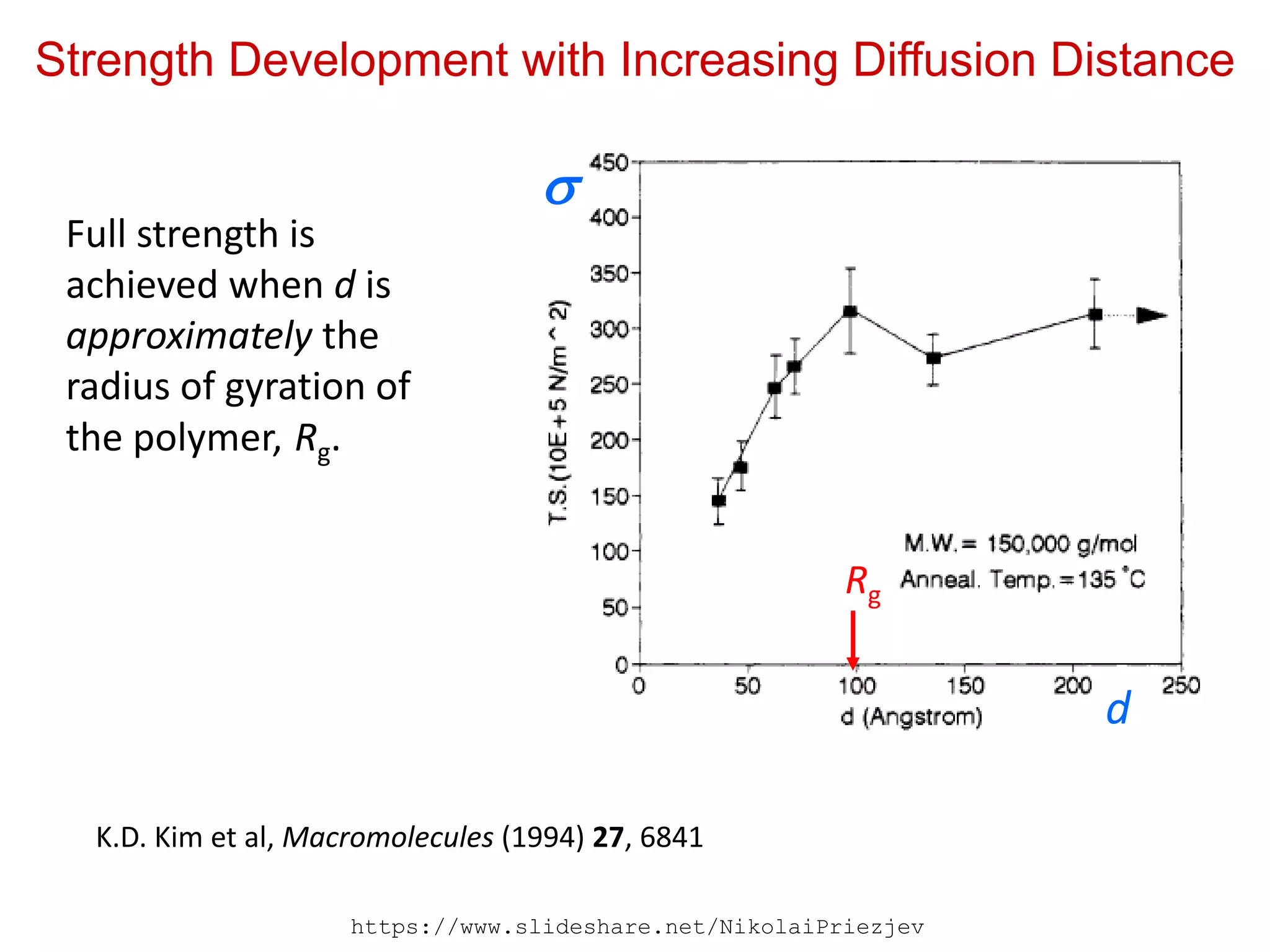
34. Strength Development with Increasing Diffusion Distance
K.D. Kim et al, Macromolecules (1994) 27, 6841
Full strength is
achieved when d is
approximately the
radius of gyration of
the polymer, Rg.
Rg
d

https://www.slideshare.net/NikolaiPriezjev