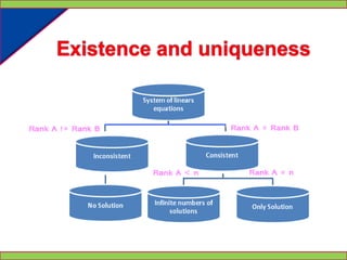
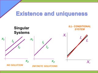
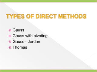
Direct methods for the solution of systems of linear equations
Definition of the problemA  x  bx=vector of independent termscoefficient matrixcoefficient matrixx=
 If b=0, the system is homogeneous
If  b!=0, the system isn’t homogeneousAugmented form of the matrix
Specials Systems
Specials Systems
Existence and uniqueness
Existence and uniquenessILL- CONDITIONAL SYSTEMSingular Systems
TYPES OF DIRECT METHODSGaussGauss with pivotingGauss - JordanThomas
GaussianeliminationIn linear algebra, Gaussian elimination is an algorithm for solving systems of linear equations, finding the rank of a matrix, and calculating the inverse of an invertible square matrix. Gaussian elimination is named after German mathematician and scientist Carl Friedrich Gauss.Elementary row operations are used to reduce a matrix to row echelon form. Gauss–Jordan elimination, an extension of this algorithm, reduces the matrix further to reduced row echelon form. Gaussian elimination alone is sufficient for many applications.
Algorithmoverview	The process of Gaussian elimination has two parts. The first part (Forward Elimination) reduces a given system to either triangular or echelon form, or results in a degenerate equation with no solution, indicating the system has no solution. This is accomplished through the use of elementary row operations. The second step uses back substitution to find the solution of the system above.	Stated equivalently for matrices, the first part reduces a matrix to row echelon form using elementary row operations while the second reduces it to reduced row echelon form, or row canonical form.	Another point of view, which turns out to be very useful to analyze the algorithm, is that Gaussian elimination computes a matrix decomposition. The three elementary row operations used in the Gaussian elimination (multiplying rows, switching rows, and adding multiples of rows to other rows) amount to multiplying the original matrix with invertible matrices from the left. The first part of the algorithm computes an LU decomposition, while the second part writes the original matrix as the product of a uniquely determined invertible matrix and a uniquely determined reduced row-echelon matrix.
OtherApplicationsFinding the inverse of a matrixSuppose A is a matrix and you need to calculate its inverse. The identity matrix is augmented to the right of A, forming a matrix (the block matrixB = [A,I]). Through application of elementary row operations and the Gaussian elimination algorithm, the left block of B can be reduced to the identity matrix I, which leaves A−1 in the right block of B.     If the algorithm is unable to reduce A to triangular form, then A is not invertible.
General algorithm to compute ranks and basesThe Gaussian elimination algorithm can be applied to any matrix A. If we get "stuck" in a given column, we move to the next column. In this way, for example, some matrices can be transformed to a matrix that has a reduced row echelon form like (the *'s are arbitrary entries). This echelon matrix T contains a wealth of information about A: the rank of A is 5 since there are 5 non-zero rows in T; the vector space spanned by the columns of A has a basis consisting of the first, third, fourth, seventh and ninth column of A (the columns of the ones in T), and the *'s tell you how the other columns of A can be written as linear combinations of the basis columns.
Gauss with pivotingAvoids the problem of division by zero orclose to zero.There are two techniquesKeep up the pivot position.Ordering the system.
Gauss Jordan Elimination Through Pivoting	A system of linear equations can be placed into matrix form. Each equation becomes a row and each variable becomes a column. An additional column is added for the right hand side. A system of linear equations and the resulting matrix are shown.The system of linear equations ...3x + 2y - 4z = 3 2x + 3y + 3z = 15 5x – 3y + z = 14becomes the augmented matrix ...
What is pivoting?     The objective of pivoting is to make an element above or below a leading one into a zero.	The "pivot" or "pivot element" is an element on the left hand side of a matrix that you want the elements above and below to be zero. Normally, this element is a one. If you can find a book that mentions pivoting, they will usually tell you that you must pivot on a one. If you restrict yourself to the three elementary row operations, then this is a true statement. However, if you are willing to combine the second and third elementary row operations, you come up with another row operation (not elementary, but still valid). 	You can multiply a row by a non-zero constant and add it to a non-zero multiple of another row, replacing that row.	So what? If you are required to pivot on a one, then you must sometimes use the second elementary row operation and divide a row through by the leading element to make it into a one. Division leads to fractions. While fractions are your friends, you're less likely to make a mistake if you don't use them. 	What's the catch? If you don't pivot on a one, you are likely to encounter larger numbers. Most people are willing to work with the larger numbers to avoid the fractions.
Thomas’ MethodADVANTAGESThe machine memory is reduced by not having to store 0's. Vectors are stored only a, b, c. Uses 3n locations instead of nxn (advantageous for n ≥ 50).Doesn’t require pivoting.Reduces the number of operations
Jacobian MethodGiven a square system of n linear equations:Ax = Bwhere:
Then A can be decomposed into a diagonal component D, and the remainder R:The system of linear equations may be rewritten as:and finally:The Jacobi method is an iterative technique that solves the left hand side of this expression for x, using previous value for x on the right hand side.
Analytically, this may be written as:The element-based formula is thus:Note that the computation of xi(k+1) requires each element in x(k) except itself. Unlike the Gauss–Seidel method, we can't overwrite xi(k) with xi(k+1), as that value will be needed by the rest of the computation. This is the most meaningful difference between the Jacobi and Gauss–Seidel methods, and is the reason why the former can be implemented as a parallel algorithm, unlike the latter. The minimum amount of storage is two vectors of size n.
AlgorithmChoose an initial guess x0 to the solutionwhile convergence not reached do	for i := 1 step until n do	σ = 0		for j := 1 step until n do			if j != i then 				end if 		end (j-loop)	end (i-loop) check if convergence is reached end (while convergence condition not reached loop)
Gauss-Seidel Method	The Gauss-Seidel method (called Seidel's method by Jeffreys and Jeffreys 1988, p. 305) is a technique for solving the equations of the linear system of equations one at a time in sequence, and uses previously computed results as soon as they are available,
	There are two important characteristics of the Gauss-Seidel method should be noted. Firstly, the computations appear to be serial. Since each component of the new iterate depends upon all previously computed components, the updates cannot be done simultaneously as in the Jacobi method. Secondly, the new iterate depends upon the order in which the equations are examined. If this ordering is changed, the components of the new iterates (and not just their order) will also change.
In terms of matrices, the definition of the Gauss-Seidel method can be expressed as where the matrices D, -L, and -U represent the diagonal, strictlylower triangular,  and strictlyupper triangularparts of A, respectively. The Gauss-Seidelmethod is applicabletostrictlydiagonallydominant, orsymmetric positive definite matrices A.
BibliographyMétodos Numéricos en Ingeniería de Petróleos. Elkin Rodolfo Santafé Rangel, lngeniero de Petróleos, Bucaramanga – Colombia © 2008http://en.wikipedia.org/wiki/Gaussian_eliminationhttp://people.richland.edu/james/lecture/m116/matrices/pivot.htmlhttp://en.wikipedia.org/wiki/Jacobi_method

Direct Methods For The Solution Of Systems Of

  • 1.
    Direct methods forthe solution of systems of linear equations
  • 2.
    Definition of theproblemA x bx=vector of independent termscoefficient matrixcoefficient matrixx=
  • 3.
    If b=0,the system is homogeneous
  • 4.
    If b!=0,the system isn’t homogeneousAugmented form of the matrix
  • 5.
  • 6.
  • 7.
  • 8.
    Existence and uniquenessILL-CONDITIONAL SYSTEMSingular Systems
  • 9.
    TYPES OF DIRECTMETHODSGaussGauss with pivotingGauss - JordanThomas
  • 10.
    GaussianeliminationIn linear algebra,Gaussian elimination is an algorithm for solving systems of linear equations, finding the rank of a matrix, and calculating the inverse of an invertible square matrix. Gaussian elimination is named after German mathematician and scientist Carl Friedrich Gauss.Elementary row operations are used to reduce a matrix to row echelon form. Gauss–Jordan elimination, an extension of this algorithm, reduces the matrix further to reduced row echelon form. Gaussian elimination alone is sufficient for many applications.
  • 11.
    Algorithmoverview The process ofGaussian elimination has two parts. The first part (Forward Elimination) reduces a given system to either triangular or echelon form, or results in a degenerate equation with no solution, indicating the system has no solution. This is accomplished through the use of elementary row operations. The second step uses back substitution to find the solution of the system above. Stated equivalently for matrices, the first part reduces a matrix to row echelon form using elementary row operations while the second reduces it to reduced row echelon form, or row canonical form. Another point of view, which turns out to be very useful to analyze the algorithm, is that Gaussian elimination computes a matrix decomposition. The three elementary row operations used in the Gaussian elimination (multiplying rows, switching rows, and adding multiples of rows to other rows) amount to multiplying the original matrix with invertible matrices from the left. The first part of the algorithm computes an LU decomposition, while the second part writes the original matrix as the product of a uniquely determined invertible matrix and a uniquely determined reduced row-echelon matrix.
  • 12.
    OtherApplicationsFinding the inverseof a matrixSuppose A is a matrix and you need to calculate its inverse. The identity matrix is augmented to the right of A, forming a matrix (the block matrixB = [A,I]). Through application of elementary row operations and the Gaussian elimination algorithm, the left block of B can be reduced to the identity matrix I, which leaves A−1 in the right block of B. If the algorithm is unable to reduce A to triangular form, then A is not invertible.
  • 13.
    General algorithm tocompute ranks and basesThe Gaussian elimination algorithm can be applied to any matrix A. If we get "stuck" in a given column, we move to the next column. In this way, for example, some matrices can be transformed to a matrix that has a reduced row echelon form like (the *'s are arbitrary entries). This echelon matrix T contains a wealth of information about A: the rank of A is 5 since there are 5 non-zero rows in T; the vector space spanned by the columns of A has a basis consisting of the first, third, fourth, seventh and ninth column of A (the columns of the ones in T), and the *'s tell you how the other columns of A can be written as linear combinations of the basis columns.
  • 14.
    Gauss with pivotingAvoidsthe problem of division by zero orclose to zero.There are two techniquesKeep up the pivot position.Ordering the system.
  • 15.
    Gauss Jordan EliminationThrough Pivoting A system of linear equations can be placed into matrix form. Each equation becomes a row and each variable becomes a column. An additional column is added for the right hand side. A system of linear equations and the resulting matrix are shown.The system of linear equations ...3x + 2y - 4z = 3 2x + 3y + 3z = 15 5x – 3y + z = 14becomes the augmented matrix ...
  • 16.
    What is pivoting? The objective of pivoting is to make an element above or below a leading one into a zero. The "pivot" or "pivot element" is an element on the left hand side of a matrix that you want the elements above and below to be zero. Normally, this element is a one. If you can find a book that mentions pivoting, they will usually tell you that you must pivot on a one. If you restrict yourself to the three elementary row operations, then this is a true statement. However, if you are willing to combine the second and third elementary row operations, you come up with another row operation (not elementary, but still valid). You can multiply a row by a non-zero constant and add it to a non-zero multiple of another row, replacing that row. So what? If you are required to pivot on a one, then you must sometimes use the second elementary row operation and divide a row through by the leading element to make it into a one. Division leads to fractions. While fractions are your friends, you're less likely to make a mistake if you don't use them. What's the catch? If you don't pivot on a one, you are likely to encounter larger numbers. Most people are willing to work with the larger numbers to avoid the fractions.
  • 17.
    Thomas’ MethodADVANTAGESThe machinememory is reduced by not having to store 0's. Vectors are stored only a, b, c. Uses 3n locations instead of nxn (advantageous for n ≥ 50).Doesn’t require pivoting.Reduces the number of operations
  • 18.
    Jacobian MethodGiven asquare system of n linear equations:Ax = Bwhere:
  • 19.
    Then A canbe decomposed into a diagonal component D, and the remainder R:The system of linear equations may be rewritten as:and finally:The Jacobi method is an iterative technique that solves the left hand side of this expression for x, using previous value for x on the right hand side.
  • 20.
    Analytically, this maybe written as:The element-based formula is thus:Note that the computation of xi(k+1) requires each element in x(k) except itself. Unlike the Gauss–Seidel method, we can't overwrite xi(k) with xi(k+1), as that value will be needed by the rest of the computation. This is the most meaningful difference between the Jacobi and Gauss–Seidel methods, and is the reason why the former can be implemented as a parallel algorithm, unlike the latter. The minimum amount of storage is two vectors of size n.
  • 21.
    AlgorithmChoose an initialguess x0 to the solutionwhile convergence not reached do for i := 1 step until n do σ = 0 for j := 1 step until n do if j != i then end if end (j-loop) end (i-loop) check if convergence is reached end (while convergence condition not reached loop)
  • 22.
    Gauss-Seidel Method The Gauss-Seidelmethod (called Seidel's method by Jeffreys and Jeffreys 1988, p. 305) is a technique for solving the equations of the linear system of equations one at a time in sequence, and uses previously computed results as soon as they are available,
  • 23.
    There are twoimportant characteristics of the Gauss-Seidel method should be noted. Firstly, the computations appear to be serial. Since each component of the new iterate depends upon all previously computed components, the updates cannot be done simultaneously as in the Jacobi method. Secondly, the new iterate depends upon the order in which the equations are examined. If this ordering is changed, the components of the new iterates (and not just their order) will also change.
  • 24.
    In terms ofmatrices, the definition of the Gauss-Seidel method can be expressed as where the matrices D, -L, and -U represent the diagonal, strictlylower triangular, and strictlyupper triangularparts of A, respectively. The Gauss-Seidelmethod is applicabletostrictlydiagonallydominant, orsymmetric positive definite matrices A.
  • 25.
    BibliographyMétodos Numéricos enIngeniería de Petróleos. Elkin Rodolfo Santafé Rangel, lngeniero de Petróleos, Bucaramanga – Colombia © 2008http://en.wikipedia.org/wiki/Gaussian_eliminationhttp://people.richland.edu/james/lecture/m116/matrices/pivot.htmlhttp://en.wikipedia.org/wiki/Jacobi_method