Chapt 6 forced heat convection (interanl flow) t

1/25/2018 Heat Transfer 1
HEAT TRANSFER
(MEng 3121)
Debre Markos University
Mechanical Engineering
Department
Prepared and Presented by:
Tariku Negash
Sustainable Energy Engineering (MSc)
E-mail: thismuch2015@gmail.com
Lecturer at Mechanical Engineering Department
Institute of Technology, Debre Markos
University, Debre Markos, Ethiopia
Jan, 2018
INTERNAL FORCED CONVECTION
Chapter 6
Laminar and Turbulent Flow in Tubes

2 2
Objectives
• Obtain average velocity from a knowledge of velocity profile, and
average temperature from a knowledge of temperature profile in
internal flow.
• Have a visual understanding of different flow regions in internal flow,
and calculate hydrodynamic and thermal entry lengths.
• Analyze heating and cooling of a fluid flowing in a tube under
constant surface temperature and constant surface heat flux conditions,
and work with the logarithmic mean temperature difference.
• Obtain analytic relations for the velocity profile, pressure drop,
friction factor, and Nusselt number in fully developed laminar flow.
• Determine the friction factor and Nusselt number in fully developed
turbulent flow using empirical relations, and calculate the heat transfer
rate.

3 3
6.1 Introduction
 Liquid or gas flow through pipes or ducts is commonly used in heating and
cooling applications and fluid distribution networks.
 The fluid in such applications is usually forced to flow by a fan or pump
through a flow section.
 Although the theory of fluid flow is reasonably well understood, theoretical
solutions are obtained only for a few simple cases such as fully developed
laminar flow in a circular pipe.
 Therefore, we must rely on experimental results and empirical relations for
most fluid flow problems rather than closed-form analytical solutions.
Circular pipes can withstand large pressure differences between the inside and
the outside without undergoing any significant distortion, but noncircular pipes
cannot.
For a fixed surface area, the circular
tube gives the most heat transfer for
the least pressure drop.

1/25/2018Heat Transfer
4
6.2 Average Velocity and Temperature in Tubes
(6.2)
(6.1)
 The fluid velocity in a pipe changes from zero at the
wall because of the no-slip condition to a maximum
at the pipe center.
 In fluid flow, it is convenient to work with an
average velocity Vavg, which remains constant in
incompressible flow when the cross-sectional area
of the pipe is constant.
 The value of the average (mean) velocity Vavg for
incompressible at some stream wise cross-section is:
6.2.1 Average Velocity

5
 But, in practice, we evaluate the fluid properties at some average
temperature and treat them as constants.
 The mean temperature Tm changes in the flow direction whenever the
fluid is heated or cooled.
(6.3)
(6.4)
 The average velocity in heating and
cooling applications may change some
what because of changes in density with
temperature.
 In fluid flow, it is convenient to work with an
average or mean temperature Tm, which
remains constant at a cross section.
6.2.1 Average Temperature

6
6.3 Laminar and Turbulent Flow in Tubes
 Flow in a tube can be laminar or turbulent, depending on the flow conditions.
 Fluid flow is streamlined and thus laminar at low velocities, but turns
turbulent as the velocity is increased beyond a critical value.
 Transition from laminar to turbulent flow does not occur suddenly; rather, it
occurs over some range of velocity where the flow fluctuates between laminar
and turbulent flows before it becomes fully turbulent.
 Most pipe flows encountered in practice are turbulent.
 Laminar flow is encountered when highly viscous fluids such as oils flow in
small diameter tubes or narrow passages.
 Transition from laminar to turbulent flow depends on the Reynolds number
as well as the degree of disturbance of the flow by surface roughness, pipe
vibrations, and the fluctuations in the flow.
 The flow in a pipe is laminar for Re < 2300,
fully turbulent for Re > 10,000, and transitional
in between.

7
6.3.1 Reynolds number for flow in a circular tube
For flow through noncircular tubes, the Reynolds
number as well as the Nusselt number, and the
friction factor are based on the hydraulic diameter
Dh
(6.5)
(6.6)

8
6.4.1 For Velocity
 Velocity boundary layer: The region of the flow in which the effects of the
viscous shearing forces caused by fluid viscosity are felt.
 The hypothetical boundary surface divides the flow in a pipe into two
regions:
 Boundary layer region: The viscous effects and the velocity changes are
significant.
 Irrotational (core) flow region: The frictional effects are negligible and the
velocity remains essentially constant in the radial direction.
6.4 The development of the Velocity and Thermal boundary layer
in a tube.

9
On the fig the development of the velocity boundary layer in a pipe:-
The developed average velocity profile is parabolic in laminar flow, as shown,
but much flatter or fuller in turbulent flow.)
 Hydrodynamic entrance region: The region from the pipe inlet to the point at
which the velocity profile is fully developed.
 Hydrodynamic entry length Lh: The length of the hydrodynamic entrance
region.
 Hydrodynamically fully developed region: The region beyond the entrance
region in which the velocity profile is fully developed and remains unchanged.

10
 Thermal entrance region: The region of flow over which the thermal
boundary layer develops and reaches the tube center.
 Thermal entry length: The length of the thermal entrance region.
 Thermally developing flow: Flow in the thermal entrance region. This
is the region where the temperature profile develops.
6.4.2 For Temperature
The fluid properties in internal flow are usually evaluated at the bulk mean fluid
temperature, which is the arithmetic average of the mean temperatures at the
inlet and the exit: Tb = (Tm, i + Tm, e)/2.

11
 Thermally fully developed region: The region beyond the thermal
entrance region in which the dimensionless temperature profile
remains unchanged.
 Fully developed flow: The region in which the flow is both hydro-
dynamically and thermally developed.

12
Hydro dynamically fully developed:
Thermally fully developed:
6.5 Analysis for Hydro dynamically and Thermally
(6.7)
the temperature profile in the thermally fully developed region may vary with x in
the flow direction. That is, unlike the velocity profile, the temperature profile can
be different at different cross sections of the tube in the developed region, and it
usually is.
However, the dimensionless temperature profile defined above remains
unchanged in the thermally developed Region when the temperature or heat
flux at the tube surface remains constant.
But,

13
 Therefore, both the friction (which is related to wall shear stress) and convection
coefficients remain constant in the fully developed region of a tube (does not
vary with x)
Surface heat flux: (6.8)
 During laminar flow in a tube, the magnitude of the dimensionless Prandtl
number (Pr), (i, e is a measure of the relative growth (thickness) of the velocity
and thermal boundary layers).
 For fluids with 𝐏𝐫 ≈ 𝟏, such as gases, the two boundary layers essentially
coincide with each other.
 For fluids with 𝑷𝒓 ≫ 𝟏, such as oils, the velocity boundary layer outgrows the
thermal boundary layer. As a result the hydrodynamic entry length is smaller
than the thermal entry length. The opposite is true for fluids with 𝑷𝒓 ≪ 𝟏 such
as liquid metals (Mercury).
Note:-Read chapt 5 lecture ppt. slide No 30 for Pr No for common fluids.

14
 The friction factor and the heat transfer
coefficient are highest at the tube inlet where
the thickness of the boundary layers is zero,
and decrease gradually to the fully
developed values, as shown in Fig.
 Therefore, the Pressure drop and heat flux
are higher in the entrance regions of a tube,
and the effect of the entrance region is
always to enhance the average friction and
heat transfer coefficients for the entire tube.
 This enhancement can be significant for short
tubes but negligible for long ones.
6.6 Entry Lengths
For hydrodynamic entry length is usually taken to
be the distance from the tube entrance where the
friction coefficient reaches within about 2 percent
of the fully developed value.
Where is the end point of entry length (numerical)?

15
In laminar flow, the hydrodynamic 𝐿ℎand thermal entry lengths 𝐿 𝑡 are given
approximately as [see Kays and Crawford (1993), and Shah and Bhatti (1987),]
6.6.1 Entry Lengths through Laminar Flow
 For Re = 20, the hydrodynamic entry length is about the size of the diameter,
but increases linearly with the velocity.
 In the limiting case of Re = 2300, the hydrodynamic entry length is 115D.
(6.9)
(6.10)
6.6.2 Entry Lengths through Turbulent Flow
 In turbulent flow, the intense mixing during random fluctuations usually
overshadows the effects of momentum and heat diffusion, and
therefore the hydrodynamic and thermal entry lengths are of about the
same size (𝑳 𝒕 = 𝑳 𝒉) and independent of the Prandtl number.

16
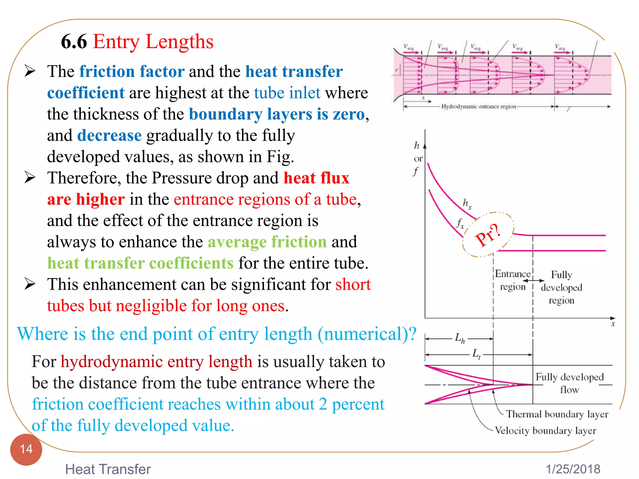
 The hydrodynamic entry length for turbulent flow can be determined
from [see Bhatti and Shah (1987), and Zhi-qing (1982)]
 The hydrodynamic entry length is much shorter in turbulent flow, as
expected, and its dependence on the Reynolds number is weaker.
 It is 11D at Re =10,000, and increases to 43D at Re = 105.
 In practice, it is generally agreed that the entrance effects are confined
within a tube length of 10 diameters, and the hydrodynamic and
thermal entry lengths are approximately taken to be
(6.11)
 Also, the friction factor and the heat transfer coefficient remain constant
in fully developed laminar or turbulent flow since the velocity and
normalized temperature profiles do not vary in the flow direction.
(6.12)

17
The Nusselt number represents the enhancement of heat
transfer through a fluid layer as a result of convection
relative to conduction across the same fluid layer.
The larger the Nusselt number, the more effective the
convection.
A Nusselt number of Nu = 1 for a fluid layer represents
heat transfer across the layer by pure conduction.
Lc is the characteristic length.
6.7.1 Introduction of Nusselt Number
Nusselt number: Dimensionless convection heat transfer coefficient.
6.7 Local Nusselt number along a tube in turbulent flow
(6.13)

18
i. The Nusselt numbers and thus the
convection heat transfer coefficients are
much higher in the entrance region.
ii. The Nusselt number reaches a constant
value at a distance of less than 10
diameters, and thus the flow can be
assumed to be fully developed for x >
10D.
iii. The Nusselt numbers for the uniform
surface temperature and uniform surface
heat flux conditions are identical in the
fully developed regions, and nearly
identical in the entrance regions.
 Therefore, Nusselt number is insensitive to the type of thermal boundary
condition, and the turbulent flow correlations can be used for either type
of boundary condition.
We make these important observations from this figure:
6.7.2 Local Nusselt number along a tube in Turbulent flow

19
The thermal conditions at the surface can
be approximated to be
• constant surface temperature
(Ts= const) or
• constant surface heat flux (qs = const).
The constant surface temperature
condition is realized when a phase
change process such as boiling or
condensation occurs at the outer surface
of a tube.
The constant surface heat flux condition
is realized when the tube is subjected to
radiation or electric resistance heating
uniformly from all directions.
We may have either Ts = constant or
qs = constant at the surface of a tube,
but not both.
The heat transfer to a fluid flowing in a
tube is equal to the increase in the energy
of the fluid.
hx is the local heat transfer coefficient.
Surface heat flux
Rate of heat transfer
6.8 General Thermal Analysis
(6.14)
(6.15)

20
Variation of the tube surface and the
mean fluid temperatures along the tube
for the case of constant surface heat
flux.
Mean fluid temperature at the tube
exit:
Rate of heat transfer:
Surface temperature:
6.8.1 Constant Surface Heat Flux ( = constant)
(6.16)
(6.17)
(6.18)

21
Energy interactions for a differential control volume in a tube.
where p is the perimeter of the tube.
Noting that both and h are constants, the
differentiation of Eq. (6.18) with respect to x
gives
Dimensionless temperature profile remains unchanged in the fully developed
region gives
(6.19)
(6.20)
(6.21)

22
Combining Eqs. (6.19), (6.20), and (6.21)
Then we conclude that in fully developed flow in a tube subjected to
constant surface heat flux, the temperature gradient is independent of x and
thus the shape of the temperature profile does not change along the tube as
shown in fig.
(6.22)
(6.23)

23
6.8.2 Constant Surface Temperature (Ts = constant)
From Newton’s law of cooling rate of heat transfer to or from a fluid
flowing in a tube
Two suitable ways of expressing Tavg:
A. Arithmetic mean temperature difference
B. Logarithmic mean temperature difference
A. Arithmetic mean temperature difference:
(6.25
(6.24)
Where, Bulk mean fluid temperature: Tb = (Ti + Te)/2
 By using arithmetic mean temperature difference, we assume that the
mean fluid temperature varies linearly along the tube, which is hardly
ever the case when Ts = constant.

24
 This simple approximation often gives acceptable results, but not
always. Therefore, we need a better way to evaluate Tavg.
 Now consider the heating of a fluid in a tube of constant cross section,
Integrating from x = 0 (tube inlet, Tm = Ti)
to x = L (tube exit, Tm = Te)
(6.27)
(6.26)
Where,
since 𝑇𝑠 is constant

25
 This relation can also be used to determine the mean fluid temperature
𝑇 𝑚(x) at any x by replacing 𝐴 𝑠 = 𝑝𝐿 𝑏𝑦 𝑝𝑥.
(6.28)
Form the fig
The temperature difference between the fluid
and the surface decays exponentially in the
flow direction, and the rate of decay depends
on the magnitude of the exponent 𝒉𝑨 𝒔/ 𝒎𝒄 𝒑
Constant temperature.- mean fluid temperature along the tube for the case of
Dimensionless temperature
𝑇𝑠−𝑇𝑒
𝑇𝑠−𝑇 𝑖
𝑖𝑠 𝑐𝑎𝑙𝑙𝑒𝑑
Number of Transfer Unit (𝑁𝑇𝑈)
 For NTU > 5, the exit temperature of
the fluid becomes almost equal to the
surface Temperature, 𝑇𝑒 ≈ 𝑇𝑠
 But the 𝑇𝑒 doesn’t cross 𝑇𝑠.
6.8.3 Number of Transfer Unit (𝑁𝑇𝑈)

26
 A small value of NTU indicates more
opportunities for heat transfer.
 When Te differs from Ti by no more
than 40 percent, the error in using the
arithmetic mean temperature
difference is less than 1 percent.
NTU: Number of transfer units.
 A measure of the effectiveness of the heat transfer systems.
 For NTU = 5, Te = Ts, and the limit for heat transfer is reached and the heat
transfer will not increase no matter how much we extend the length of the
tube.
 An NTU greater than 5 indicates that the fluid flowing in a tube will
reach the surface temperature at the exit regardless of the inlet
temperature.

27
B. Log mean temperature difference
Solving Eq. (6.27) for 𝑚𝑐 𝑝
Substituting this into Eq. (6.16), we obtain
Where,
is the logarithmic mean temperature difference
 Tln is an exact representation of the average temperature difference between
the fluid and the surface.
(6.29)

28
6.9 Laminar Flow In Tubes
 Flow in tubes is laminar for Re < 2300, and that the flow is fully
developed if the tube is sufficiently long (relative to the entry length) so
that the entrance effects are negligible.
 In fully developed laminar flow, each fluid particle moves at a constant
axial velocity along a streamline and the velocity profile V(r) remains
unchanged in the flow direction.
 Now consider a ring-shaped differential volume
element of radius r, thickness dr, and length dx
oriented coaxially with the tube, as shown in Figure
 There is no motion in the radial direction, and thus
the velocity component v in the direction normal to
flow is everywhere zero.
 There is no acceleration since the flow is steady.
6.9.1 The relation of mean velocity to the maximum velocity

29
 The volume element involves only pressure (the product of the pressure at the
centroid of the surface and the surface area) and viscous effects, and thus the
pressure and shear forces must balance each other.
 A force balance on the volume element in the flow
direction gives which indicates that in fully developed
flow in a tube, the viscous and pressure forces
balance each other.
 Dividing by 2𝝅drdx and rearranging,
 Taking the limit as dr, dx → 0 gives
(6.30)
(6.31)
The above equation can be solved by
rearranging and integrating it twice to give
(6.32)
(6.33)

30
 Therefore, the velocity profile in fully developed laminar flow in a tube is
parabolic with a maximum at the centerline and minimum at the tube surface.
 Also, the axial velocity is positive for any r, and thus the axial pressure
gradient dP/dx must be negative (i.e., pressure must decrease in the flow
direction because of viscous effects).
(6.34)
 The mean velocity is determined from its definition by substituting Eq.
(6.34) into Eq. (6.1), and performing the integration. It gives
(6.1)𝑉𝑎𝑣𝑔
(6.35)

31
Combining the last two equations, the velocity profile is obtained to be
The maximum velocity occurs at the centerline, r = 0:
Therefore, the mean velocity is one-half of the maximum velocity.
(6.36)
(6.37)

32
6.9.2 Laminar Flow Pressure Drop
 A quantity of interest in the analysis of pipe flow is the pressure drop P since it
is directly related to the power requirements of the fan or pump to maintain flow.
 We note that dP/dx = constant, and integrate it from x = 0 where the pressure is
𝑃1 to x = L where the pressure is 𝑃2. We get
Note that in fluid mechanics, the pressure drop ∆𝑃 is a positive quantity, and is
defined as ∆𝑃 = 𝑃1 − 𝑃2.
Substitute Eqn. (6.38) in to qua (6.35) and the pressure drop
(6.38)
(6.39)
(6.40)
(who first studied experimentally the effects of roughness on tube resistance)

33
Where, in laminar flow, the friction factor is a function of the Reynolds number
only and is independent of the roughness of the pipe surface.
Head loss
Pressure losses are commonly expressed in terms of the
equivalent fluid column height, called the head loss hL.
The head loss hL represents the additional height that the fluid needs to be raised by
a pump in order to overcome the frictional losses in the pipe.
(6.41)
(6.42)
In practice, it is found convenient to express the pressure
drop and Head loss for all types of internal flows (laminar
or turbulent flows, circular or noncircular tubes, smooth or
rough surfaces) as

34
The required pumping power to overcome the pressure loss:
Where the volume flow rate ( 𝑉) of flow, which is expressed as
This equation is known as the Poiseuille’s Law, and this flow is called the
Hagen–Poiseuille flow
The average velocity for laminar flow
(6.43)
(6.44)
(6.45)
Note from Eq. (33) that for a specified flow rate, the pressure drop and thus the
required pumping power is proportional to the length of the tube and the viscosity
of the fluid, but it is inversely proportional to the fourth power of the radius (or
square diameter) of the tube.
valid for both laminar and turbulent
flows in circular and noncircular tubes.

35
 Therefore, the pumping power requirement for a piping system can be
reduced by a factor of 16 by doubling the tube diameter.
 Of course the benefits of the reduction in the energy costs must be
weighed against the increased cost of construction due to using a larger
diameter tube.
 The pressure drop is caused by viscosity, and
it is directly related to the wall shear stress.
 For the ideal inviscid flow, the pressure drop
is zero since there are no viscous effects.

36
6.9.3 Temperature Profile and the Nusselt Number for laminar flow
Noting that energy is transferred by mass in the x-direction, and by conduction in
the r-direction (heat conduction in the x-direction is assumed to be negligible), the
steady-flow energy balance for a cylindrical shell element of thickness dr and
length dx can be expressed as
Substituting and dividing by 2𝜋rdrdx gives, after rearranging,
Substituting and using
(6.46)
Fourier laws,

37
For Constant Surface Heat Flux
For fully developed flow in a circular pipe subjected to constant surface heat
flux, we have, from previous equation (6.23).
Substituting Eq. 6.23 and the relation for velocity profile (Eq. 6.36) into Eq. (6.46)
gives
Obtained by separating the variables and integrating twice to be
(6.36)
(6.23).
(6.47)
(6.48)

38
Applying the boundary conditions T/x = 0 at r = 0 (because of symmetry)
and T = Ts at r = R:
The bulk mean temperature 𝑇 𝑚 is determined by substituting the velocity
and
temperature profile relations (Eqs. 6.36 and 6.49) into Eq. (6.4) and
performing the integration. It gives
(6.49)
Combining this relation with
or
 Therefore, for fully developed laminar flow in a circular tube subjected
to constant surface heat flux, the Nusselt number is a constant.
 There is no dependence on the Reynolds or the Prandtl numbers.
(6.50)
(6.51)
(6.4)
(6.52)

39
For Constant Surface Temperature
 Asimilar analysis can be performed for
fully developed laminar flow in a
circular tube for the case of constant
surface temperature 𝑇𝑠.
 The solution procedure in this case is
more complex as it requires iterations,
but the Nusselt number relation obtained
is equally simple (Fig):
 For laminar flow with constant surface temperature, the effect of surface
roughness on the friction factor and the heat transfer coefficient is
negligible.
(6.53)

40
Nusselt number relations are
given in Table for fully
developed laminar flow in
tubes of various cross
sections.
The Reynolds and Nusselt
numbers for flow in these
tubes are based on the
hydraulic diameter Dh =
4Ac/p.
Once the Nusselt number is
available, the convection heat
transfer coefficient is
determined from h = kNu/Dh.
6.9.4 Laminar Flow in Noncircular Tubes

41
6.9.5 Developing Laminar Flow in the Entrance Region
 For a circular tube of length L subjected to constant surface temperature,
the average Nusselt number for the thermal entrance region can be determined
from:
 The average Nusselt number is larger at the entrance region, and it
approaches asymptotically to the fully developed value of 3.66 as L → .
 When the difference between the surface and the fluid temperatures is large, it
may be necessary to account for the variation of viscosity with temperature:
All properties are evaluated at the bulk mean
fluid temperature, except for s, which is
evaluated at the surface temperature.
 The average Nusselt number for the thermal entrance region of flow between
isothermal parallel plates of length L is
(6.54)
(6.55)

42
 Most correlations for the friction and heat transfer coefficients in turbulent flow
are based on experimental studies because of the difficulty in dealing with
turbulent flow theoretically.
 For smooth tubes, the friction factor in turbulent flow can be determined from
the explicit first Petukhov equation [Petukhov (1970),] given as
6.10 Turbulent Flow In Tubes
The Nusselt number in turbulent flow is related to the friction factor through
the Chilton–Colburn analogy expressed as
 Once the friction factor is available, this equation can be used conveniently to
evaluate the Nusselt number for both smooth and rough tubes.
 For fully developed turbulent flow in smooth tubes, a simple relation for the
Nusselt number can be obtained by substituting the simple power law relation
6.10.1 Nusselt number for turbulent flow
(5.57)
(5.58)
(6.56)

43
Colburn equation
The accuracy of this equation can be improved by modifying it as
where n=0.4 for heating and 0.3 for cooling of the fluid flowing through the tube.
Dittus–Boelter equation
When the variation in properties is large due to a large temperature difference:
All properties are evaluated at Tb except s, which is evaluated at Ts.
Second
Petukhov
equation
(5.59)
(5.60)
(5.61)
(5.62)

44
Gnielinski
relation
The relations above are not very sensitive to the thermal conditions at the tube
surfaces and can be used for both Ts = constant and qs = constant.
(5.63)
(5.64)

45
6.10.2 Rough Surfaces effect on Turbulent flow
The friction factor in fully developed turbulent pipe flow depends on the Reynolds
number and the relative roughness  /D, which is the ratio of the mean height of
roughness of the pipe to the pipe diameter.
Colebrook equation
Moody chart is given in the appendix.
It presents the Darcy friction factor for pipe flow as a function of the Reynolds
number and  /D over a wide range.
An approximate explicit relation for f
was given by S. E. Haaland.
 In turbulent flow, wall roughness increases the heat transfer coefficient h by a
factor of 2 or more.
 The convection heat transfer coefficient for rough tubes can be calculated
approximately from the Gnielinski relation or Chilton–Colburn analogy by using
the friction factor determined from the Moody chart or the Colebrook equation.
(5.65)
(5.66)

47
6.10.3 Developing Turbulent Flow in the Entrance Region
 The entry lengths for turbulent flow are typically short, often just 10 tube diameters long,
and thus the Nusselt number determined for fully developed turbulent flow can be used
approximately for the entire tube.
 This simple approach gives reasonable results for pressure drop and heat transfer for long
tubes and conservative results for short ones.
 Correlations for the friction and heat transfer coefficients for the entrance regions are
available in the literature for better accuracy.
6.10.4 Turbulent Flow in Noncircular Tubes
In turbulent flow, the velocity profile
is nearly a straight line in the core
region, and any significant velocity
gradients occur in the viscous
sublayer.
Pressure drop and heat transfer characteristics of
turbulent flow in tubes are dominated by the very
thin viscous sublayer next to the wall surface, and
the shape of the core region is not of much
significance.
The turbulent flow relations given above for
circular tubes can also be used for noncircular
tubes with reasonable accuracy by replacing the
diameter D in the evaluation of the Reynolds
number by the hydraulic diameter Dh = 4Ac/p.

48
6.10.5 Flow through Tube Annulus
Some simple heat transfer equipments consist of two
concentric tubes, and are properly called double-tube
heat exchangers (Fig.).
Hydraulic diameter of annulus
 The Nusselt numbers for fully developed
laminar flow with one surface isothermal and
the other adiabatic are given in Table.
 When Nusselt numbers are known, the
convection coefficients for the inner and the
outer surfaces are determined from
Table
 For laminar flow, the convection coefficients for the
inner and the outer surfaces are determined from
(5.67)
(5.68)

49
 For fully developed turbulent flow, hi and ho are approximately equal
to each other, and the tube annulus can be treated as a noncircular
duct with a hydraulic diameter of Dh = Do − Di.
 The Nusselt number can be determined from a suitable turbulent flow
relation such as the Gnielinski equation.
 To improve the accuracy, Nusselt numbers can be multiplied by the
following correction factors when one of the tube walls is adiabatic
and heat transfer is through the other wall:
(5.69)

50
6.10.6 Heat Transfer Enhancement
 Tubes with rough surfaces have much
higher heat transfer coefficients than tubes
with smooth surfaces.
 Heat transfer in turbulent flow in a tube
can be increased by as much as 400
percent by roughening the surface.
 Roughening the surface, of course, also
increases the friction factor and thus the
power requirement for the pump or the fan.
 The convection heat transfer coefficient
can also be increased by inducing
pulsating flow by pulse generators, by
inducing swirl by inserting a twisted
tape into the tube, or by inducing
secondary flows by coiling the tube.

51
Water enters a 2.5-cm-internal-diameter thin copper tube of a heat
exchanger at 15°C at a rate of 0.3 kg/s, and is heated by steam condensing
outside at 120°C. If the average heat transfer coefficient is 800 W/𝑚2
℃,
determine the length of the tube required in order to heat the water to
115°C
Example 6–1
Assumptions
1 Steady operating conditions exist.
2 Fluid properties are constant.
3 The convection heat transfer coefficient is
constant.
4 The conduction resistance of copper tube is
negligible so that the inner surface
temperature of the tube is equal to the
condensation temperature of steam.

52
Water is to be heated from 15°C to 65°C as it flows through a 3-cm-internal
diameter 5-m-long tube as shon on the fig. The tube is equipped with an
electric resistance heater that provides uniform heating throughout the
surface of the tube. The outer surface of the heater is well insulated, so that
in steady operation all the heat generated in the heater is transferred to the
water in the tube. If the system is to provide hot water at a rate of 10 L/min,
determine the power rating of the resistance heater. Also, estimate the inner
surface temperature of the pipe at the exit.
Example 6–2
Assumptions 1 Steady flow conditions exist. 2
The surface heat flux is uniform.
3 The inner surfaces of the tube are smooth
The properties of water at the bulk mean temperature of Tb=40 °C

53
Assumptions:
1. Steady-state conditions.
2. Uniform heat flux.
3. Incompressible liquid and negligible viscous dissipation.
4. Constant properties.
5. Adiabatic outer tube surface.
Properties:
Example 6–3

54
Cooling water available at 10°C is used to condense steam at 30°C in the
condenser of a power plant at a rate of 0.15 kg/s by circulating the cooling water
through a bank of 5-m-long 1.2-cm-internal-diameter thin copper tubes. Water
enters the tubes at a mean velocity of 4 m/s, and leaves at a temperature of 24°C.
The tubes are nearly isothermal at 30°C. Determine
a) the average heat transfer coefficient between the water and the tubes, and
b) the number of tubes needed to achieve the indicated heat transfer rate in the
condenser
c) Repeat Example 6.4 for steam condensing at a rate of 0.60 kg/s.
Example 6–4
Assumptions
2 The surface temperature of the pipe is constant.
3 The thermal resistance of the pipe is negligible.

55
Consider an air solar collector that is 1 m wide and 5 m long and has a constant
spacing of 3 cm between the glass cover and the collector plate. Air enters the
collector at 30°C at a rate of 0.15 m /s through the 1-m-wide edge and flows
along the 5-m-long passage way. If the average temperatures of the glass cover
and the collector plate are 20°C and 60°C, respectively, determine
(a) the net rate of heat transfer to the air in the collector and
(b) the temperature rise of air as it flows through the collector.
Example 6–5
Assumptions
2 The inner surfaces of the spacing are
smooth.
3 Air is an ideal gas with constant
properties.
4 The local atmospheric pressure is 1 atm.

56
The compressed air requirements of a manufacturing facility are met by a 150-hp
compressor located in a room that is maintained at 20°C. In order to minimize the
compressor work, the intake port of the compressor is connected to the outside
through an 11-m-long, 20-cm-diameter duct made of thin aluminum sheet. The
compressor takes in air at a rate of 0.27 𝑚3/s at the outdoor conditions of 10°C and
95 kPa. Dis-regarding the thermal resistance of the duct and taking the heat
transfer coefficient on the outer surface of the duct to be 10 W/m °C, determine
(a) the power used by the compressor to overcome the pressure drop in this duct,
(b) the rate of heat transfer to the incoming cooler air, and
(c) the temperature rise of air as it flows through the duct.
Assumptions
1 Steady flow conditions exist.
2 The inner surfaces of the duct are smooth.
3 The thermal resistance of the duct is negligible.
4 Air is an ideal gas with constant properties.
Example 6–6
The properties of air:

57
Reference
This heat transfer lecture power point adapted from
1. Yunus Cengel, Heat and Mass Transfer A Practical Approach, 3rd
edition
2. Frank P. Incropera, Theodore l. Bergman, Adrienne S. Lavine,
and David P Dewitt, fundamental of Heat and Mass Transfer, 7th
edition
3. Lecture power point of heat transfer by Mehmet Kanoglu
University of Gaziantep.
You can download the previous lecture slide by using below link:
https://www.slideshare.net/TarikuNegash/chapter-4-transient-heat-
condution?qid=06cf696e-622b-45ac-ae41-cc4aa8067154&v=&b=&from_search=1
https://www.slideshare.net/TarikuNegash/two-dimensional-steady-state-heat-conduction
https://www.slideshare.net/TarikuNegash/heat-transfer-chapter-one-and-two-81503043

Chapt 6 forced heat convection (interanl flow) t

More Related Content

What's hot

Similar to Chapt 6 forced heat convection (interanl flow) t

Recently uploaded

Chapt 6 forced heat convection (interanl flow) t

Editor's Notes