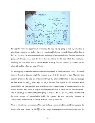
The document provides an index for a course on transport phenomena, outlining topics over 12 weeks that cover concepts like Newton's law of viscosity, shell momentum balance, boundary layers, and mass transfer. Key aspects of transport phenomena are discussed, including the governing equations for momentum, heat, and mass transfer as well as the boundary layer concept. Dimensionless groups and their importance in understanding similarity between different transport processes are also highlighted.

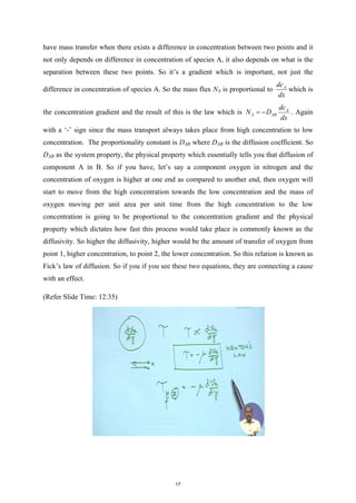
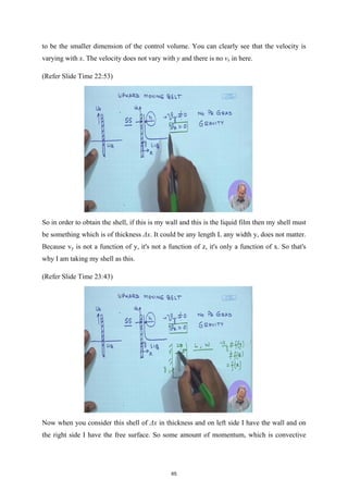
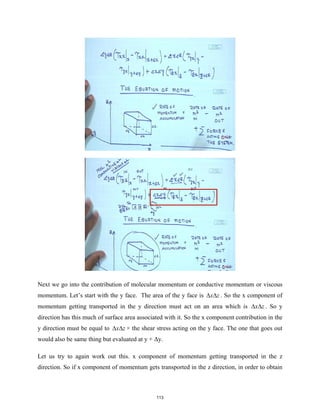
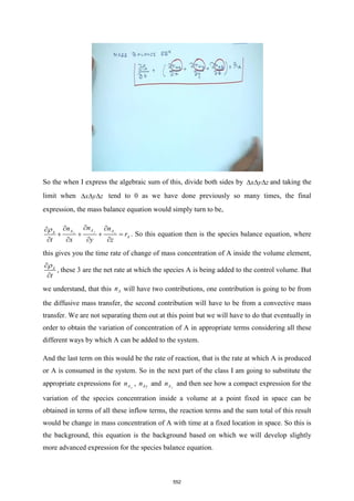
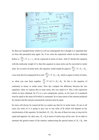
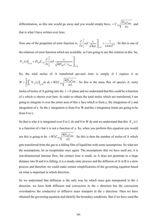
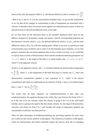
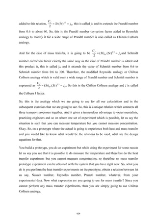
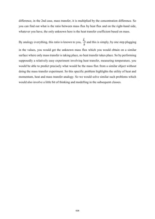
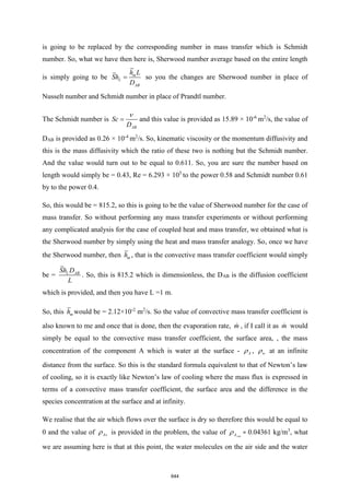
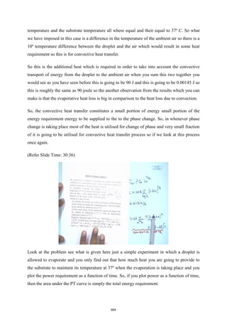
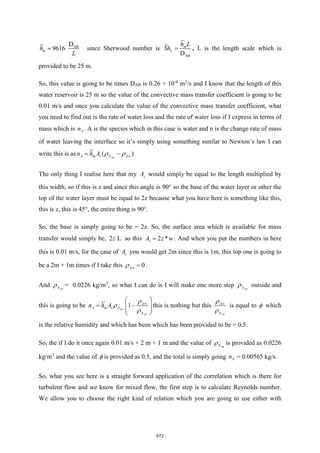
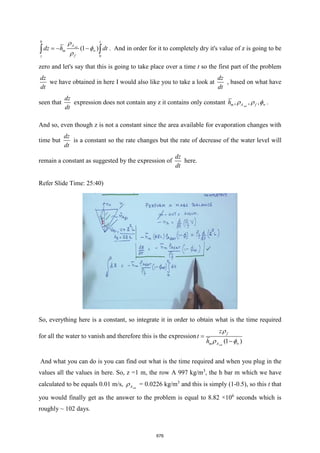
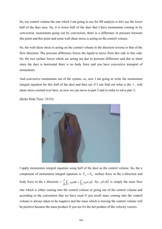
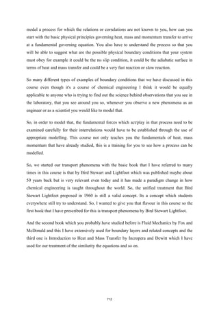
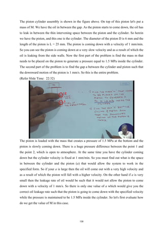
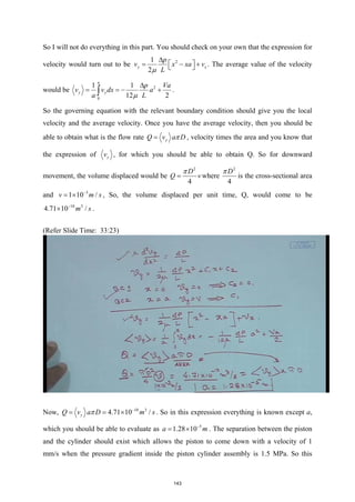
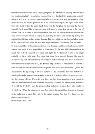
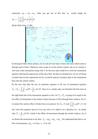
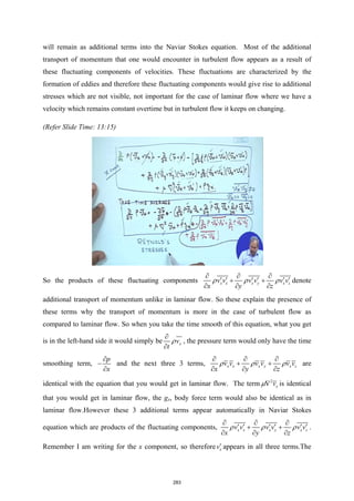
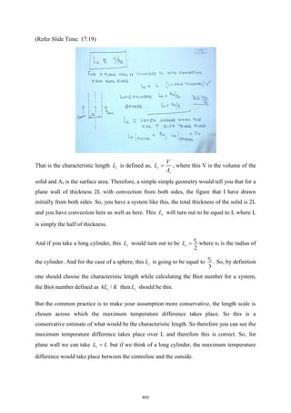
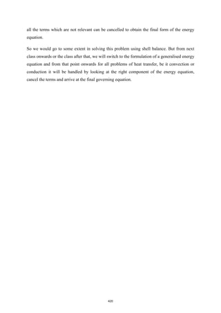
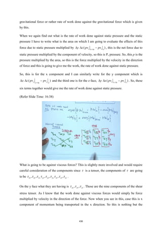
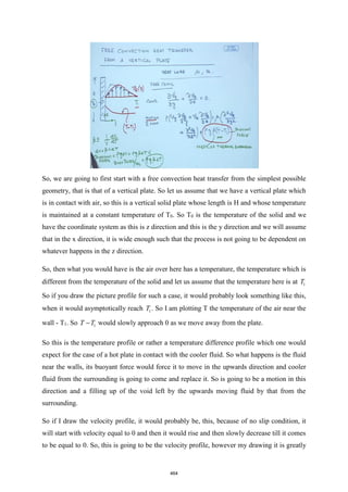
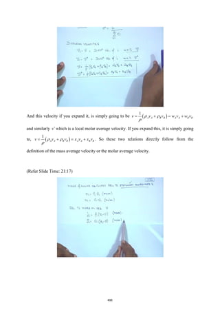
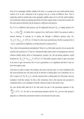
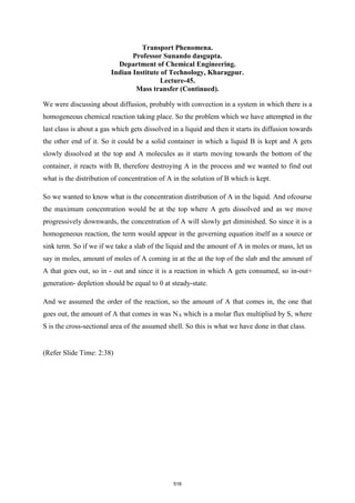
![inside the control volume would simply be ( )
x
x y z v
t
ρ
∂
∆ ∆ ∆
∂
kg/m2
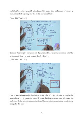
s. So if I take the convective
momentum, conductive momentum, the x component of the pressure force, the x component of
the body force and the rate of accumulation of the x momentum, then according to the equation,
which we have written,
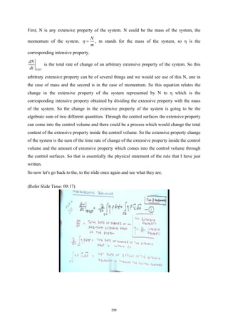
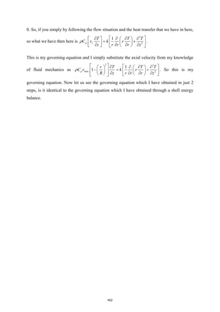
Rate of momentum Rate of momentum Rate of momentum Forces acting on
= -
accumulation coming in going out the system
+ ∑
all these terms together can be written and I am not going to write the full form of the
expression.
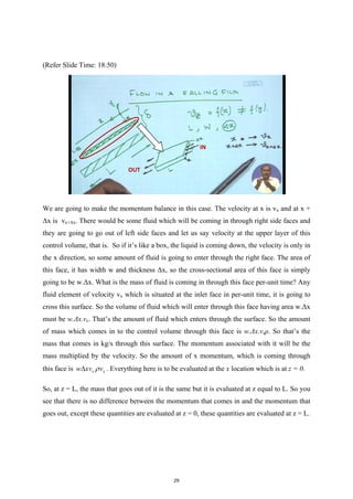
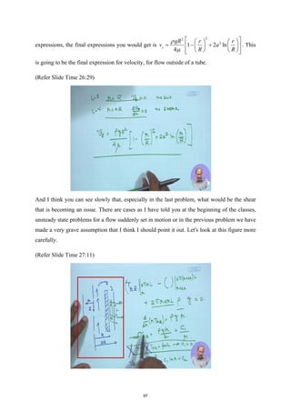
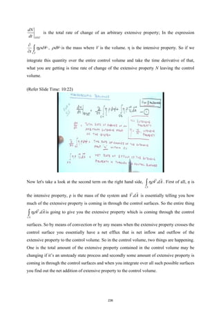
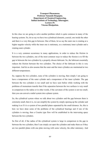
(Refer Slide Time: 21:00)
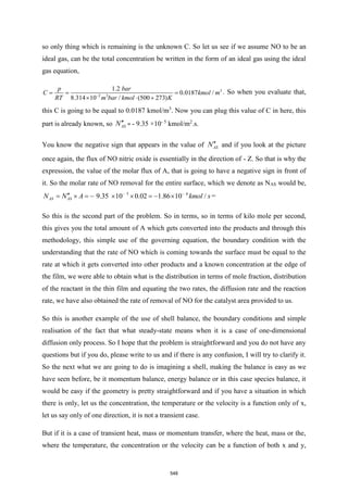
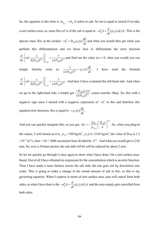
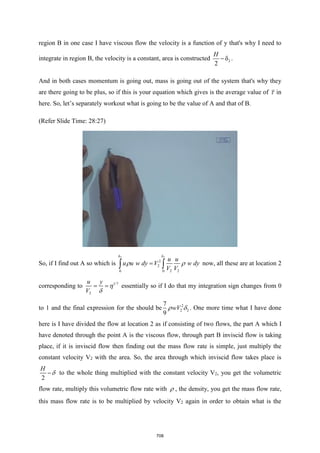
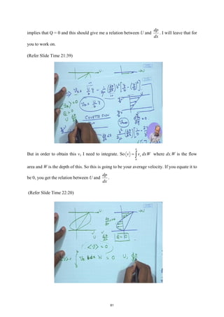
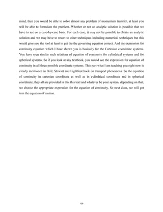
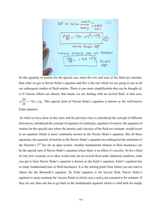
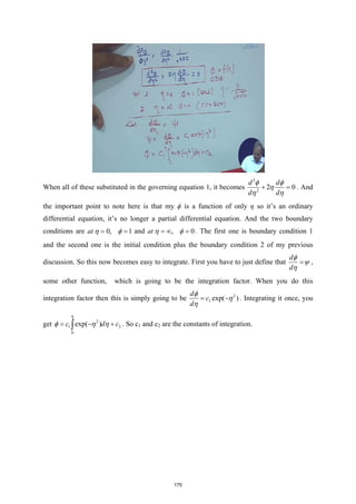
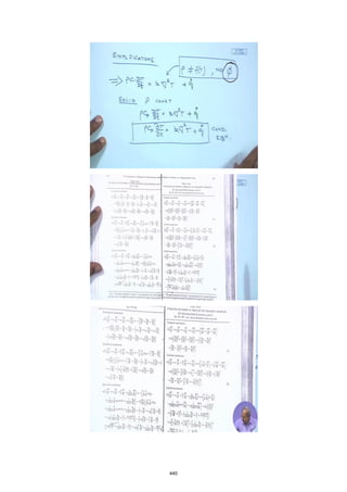
What I am going to do is I am going to simply give you the compact form of this equation after
some simplification which is [ ]
.
Dv
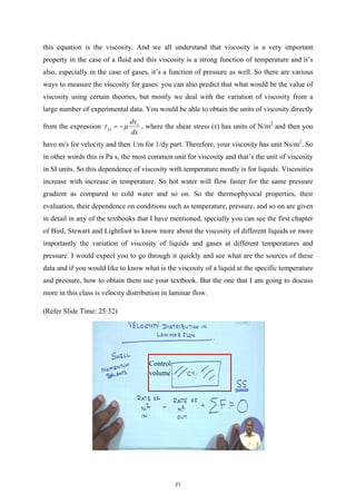
p g
Dt
ρ τ ρ
= −∇ − ∇ + . This equation in tensor notation is
known as the equation of motion, where the
Dv
Dt
ρ is essentially
mass per unit volume(
ρ)×acceleration
Dv
Dt
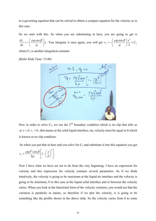
. p
∇ is pressure, Newton, force per unit volume.
Then you have .τ
∇ which is ( )
x
τ
∂
∂
, shear force per unit volume and g
ρ is gravitational force
116](https://image.slidesharecdn.com/npteltpnotesfull-220501122717/85/NPTEL-TP-Notes-full-pdf-120-320.jpg)
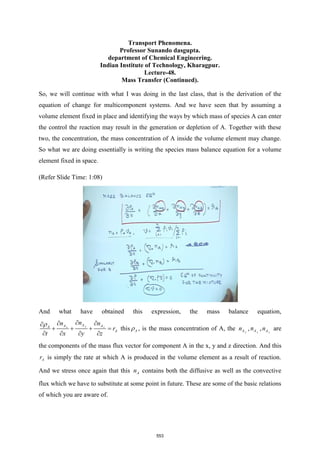
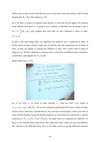
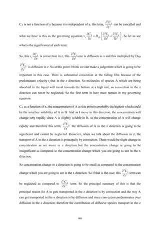
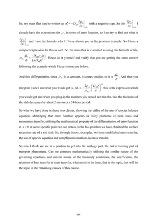
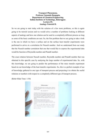
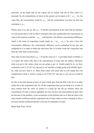
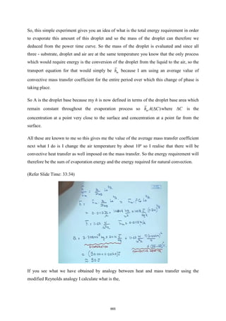
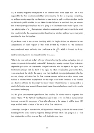
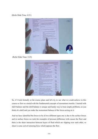
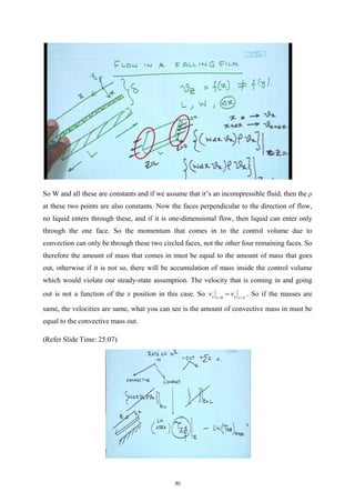
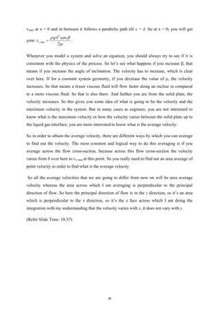
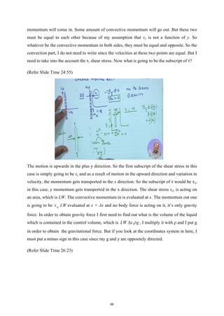
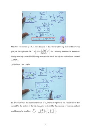
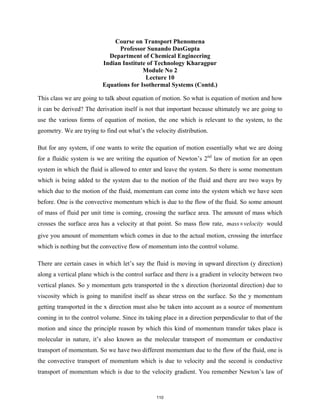
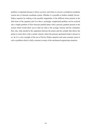
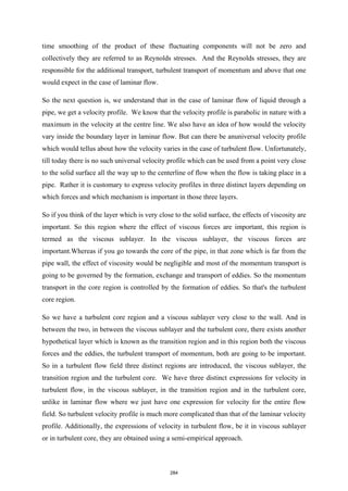
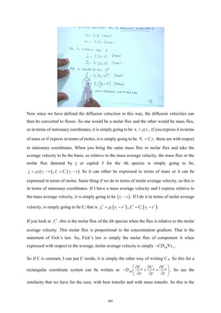
![Transport Phenomena
Prof. Sunando DasGupta
Department of Chemical Engineering
Indian Institute of Technology, Kharagpur
Lecture 11
Equations of Change for Isothermal Systems (Cont.)
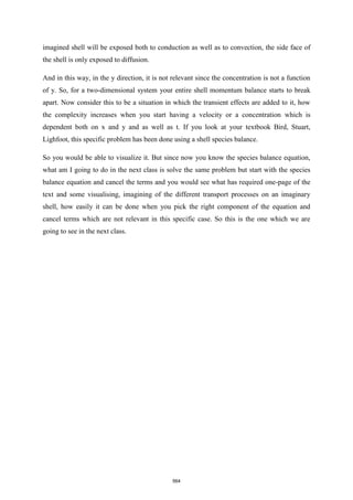
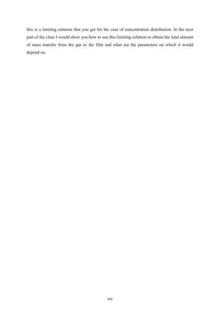
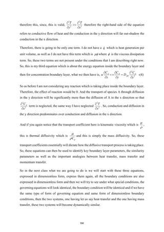
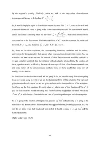
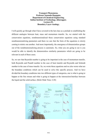
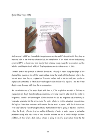
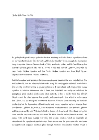
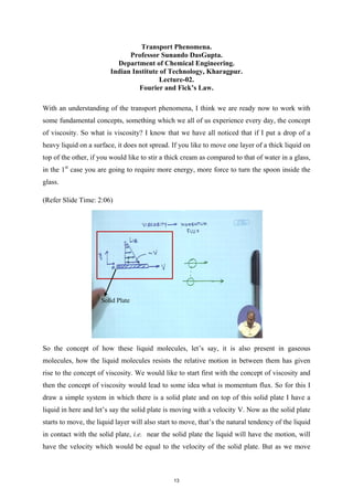
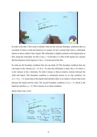
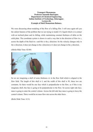
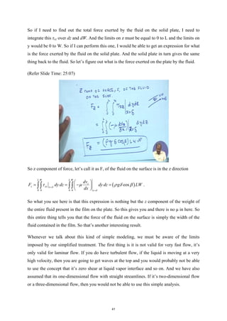
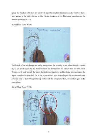
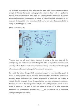
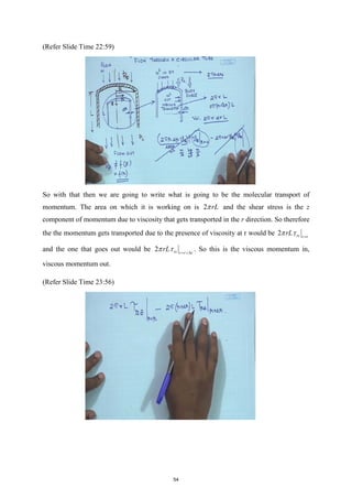
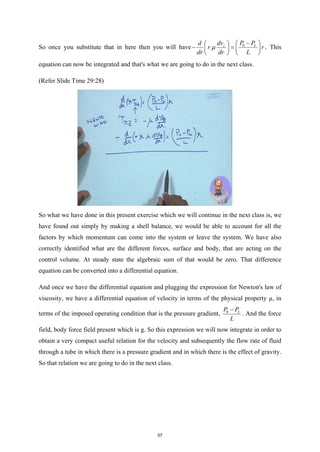
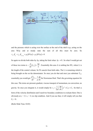
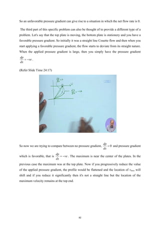
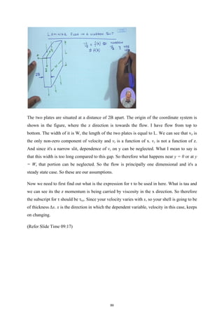
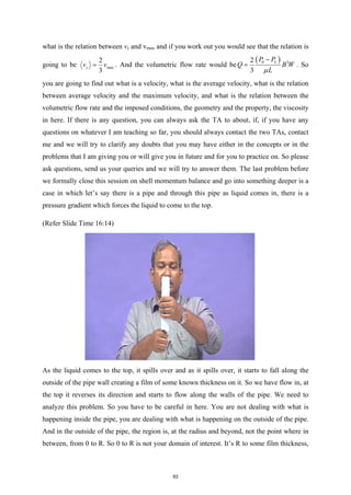
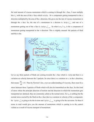
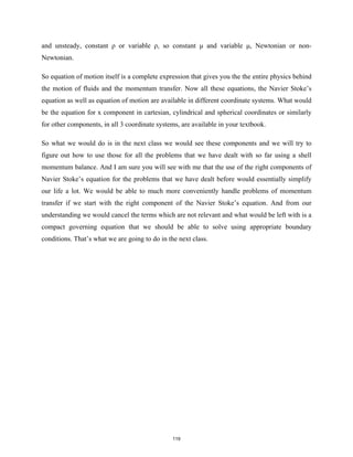
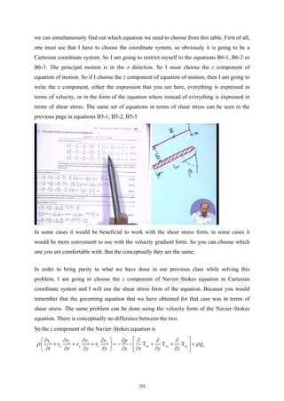
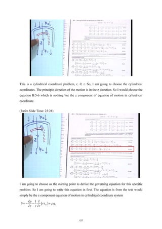
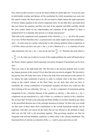
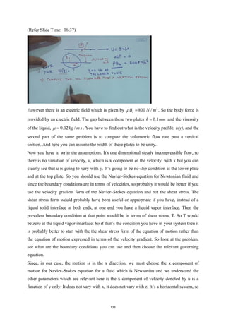
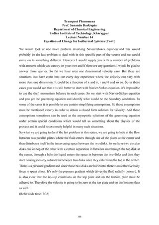
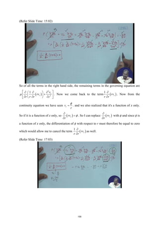
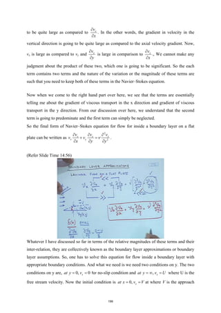
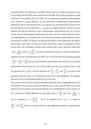
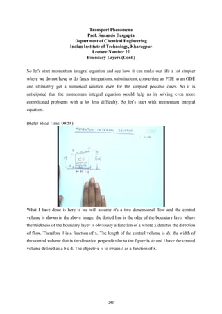
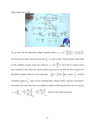
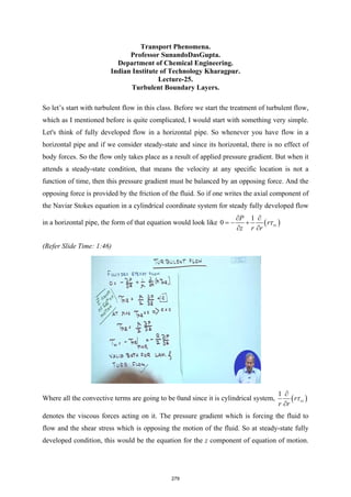
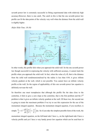
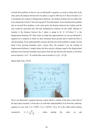
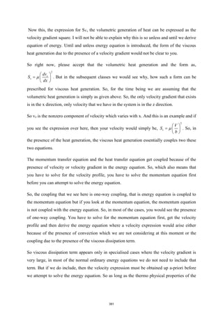
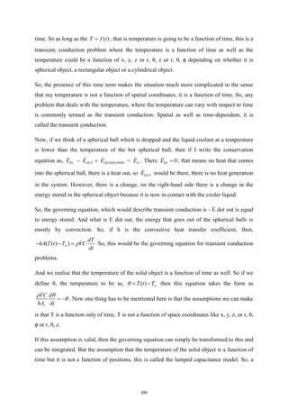
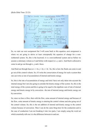
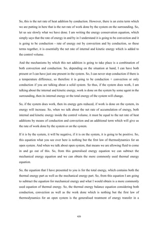
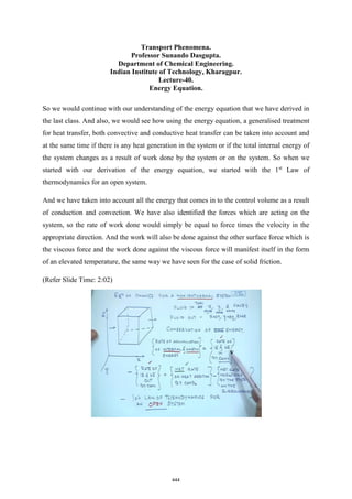
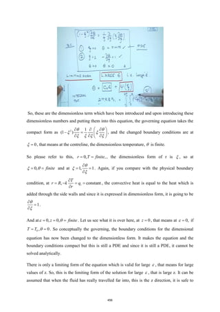
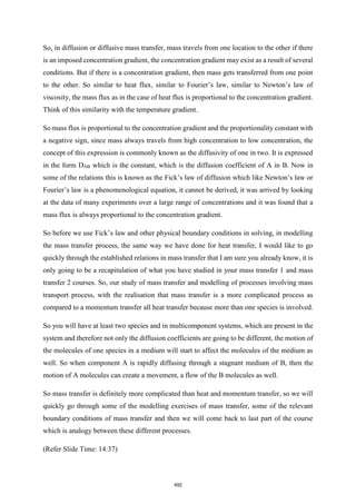
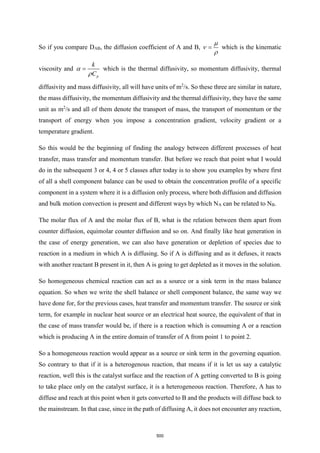
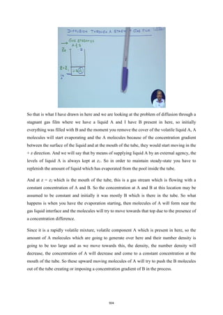
This is going to be a tutorial class on the concept that we have covered in, for equations of
motion, mostly Navier–Stokes equation. What we have seen in the previous two classes is the
fundamental concepts of derivatives, they are different types. The equations of continuity and
the equation of motion, we have a comprehensive system right now which could address any
of the fluid mechanics problems at least up to the point of governing equation. The concepts
behind choosing the boundary condition will remain unchanged from whatever we have
discussed previously. So just a quick recapitulation of what we have done over here is, we
have seen the equation of motion [ ]
.
Dv
p g
Dt
ρ τ ρ
= −∇ − ∇ + . When in the equation of motion
you add the constant ρ and constant μ and equation of continuity what you get is Navier–
Stokes equation 2
Dv
p v g
Dt
ρ µ ρ
= −∇ + ∇ + .
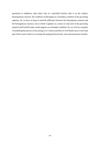
So
Dv
Dt
ρ is mass per unit volume multiplied by acceleration, so this becomes force per unit
volume. Similarly, p
∇ is also force due to pressure per unit volume. 2
v
µ∇ is viscous force
per unit volume and ρg is the gravitational force or the body force per unit volume. So all
terms in Navier–Stokes equation are nothing but force per unit volume. And the special case
would emerge if you assume that it is an inviscid fluid or the viscosity of fluid is
insignificant. What you get from Navier–Stokes equation is something which is known as
Euler's equation for inviscid flow of liquids
Dv
p g
Dt
ρ ρ
= −∇ + where this μ term would
simply be dropped. Now the expressions for different components, x, y, z components of
Navier–Stokes equation in Cartesian, cylindrical and spherical coordinates are given in any
textbook. You can refer either to Bird, Stewart and Lightfoot or or Fox McDonald, or any of
the textbooks will contain the expression for Navier–Stokes equation in different coordinate
systems.
So what you need to do in that is first see what kind of geometry you have in hand. Then
accordingly choose whether it is Cartesian, spherical or cylindrical coordinate has to be
120](https://image.slidesharecdn.com/npteltpnotesfull-220501122717/85/NPTEL-TP-Notes-full-pdf-124-320.jpg)
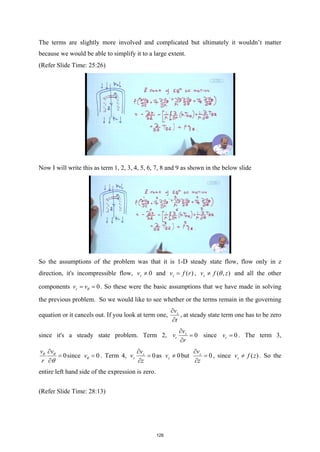
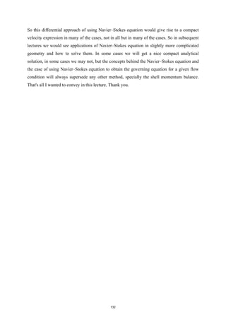
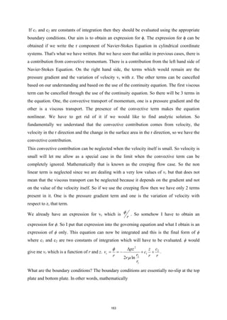
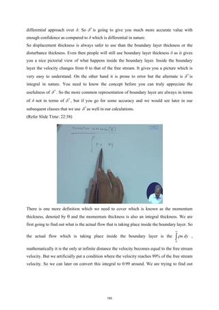

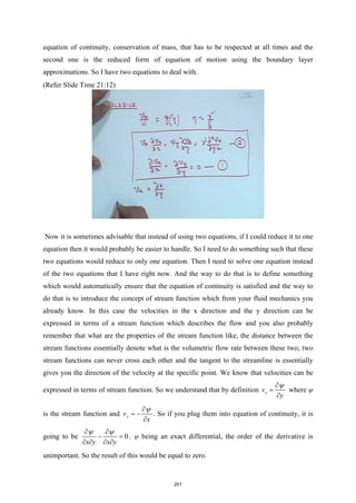
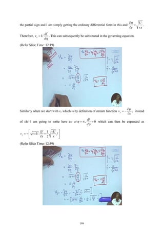
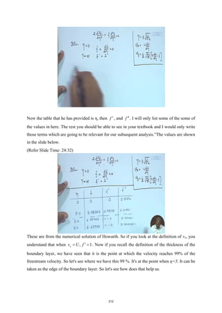
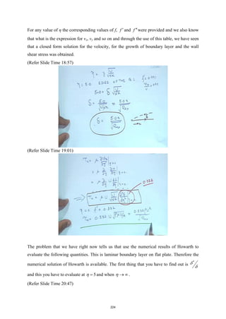
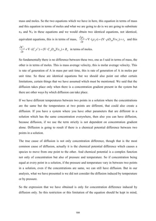
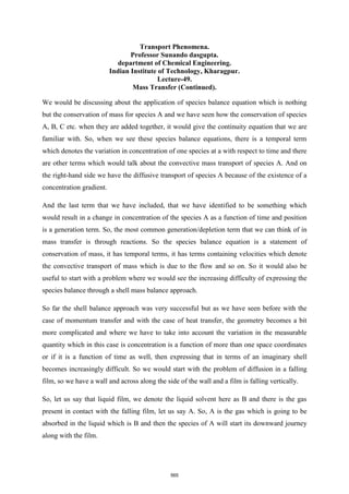
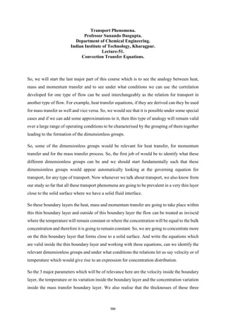
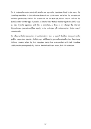
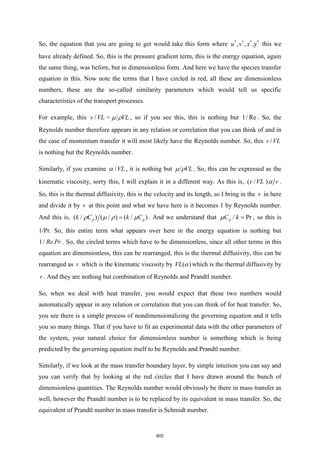
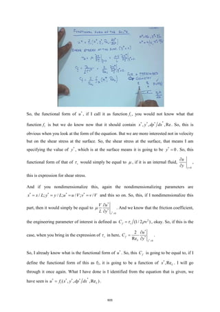
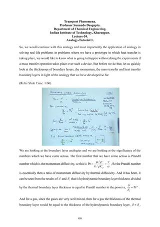
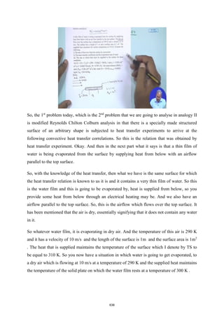
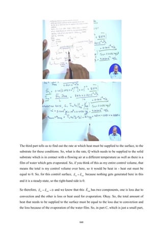
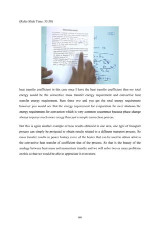
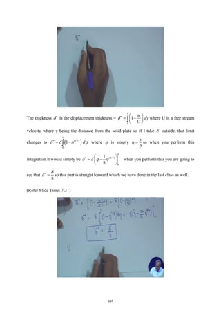
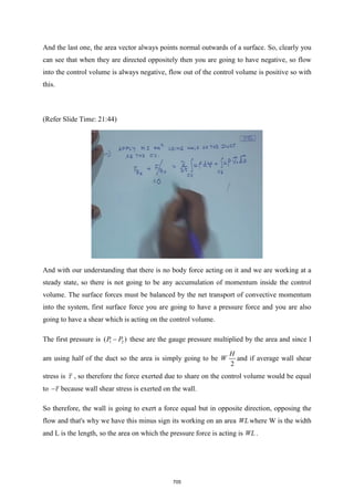
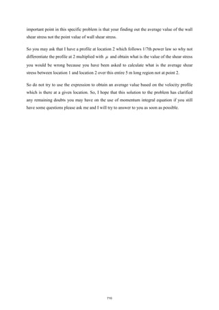
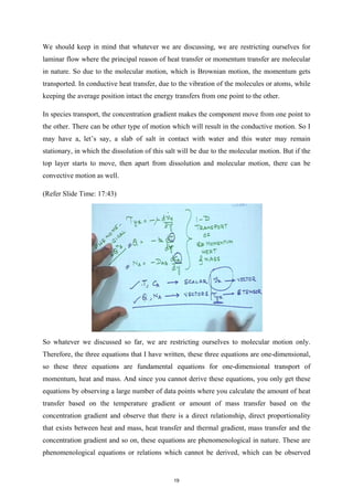
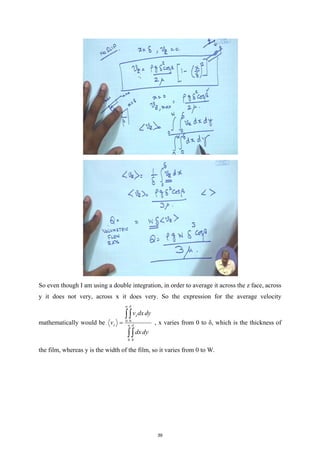
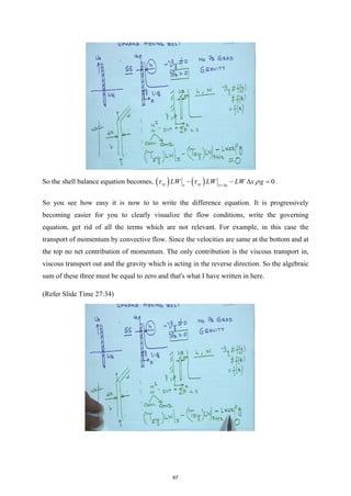
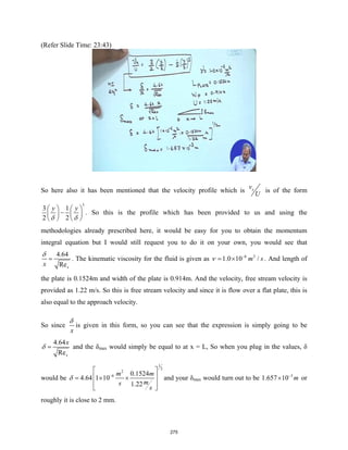
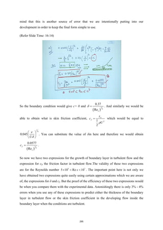
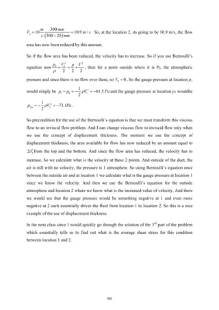
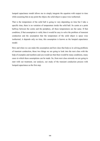
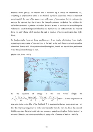
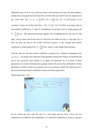
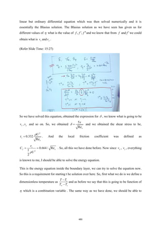
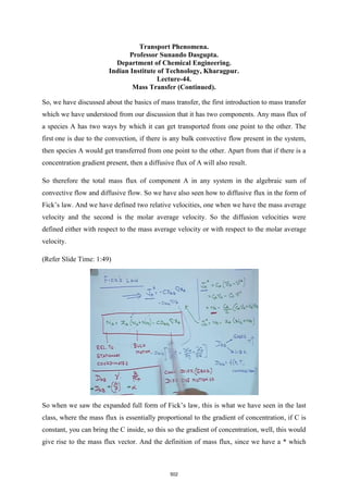
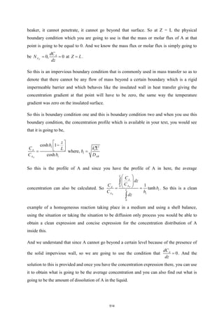
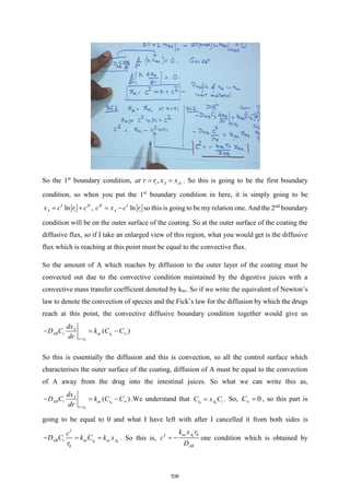
![For 5
η = , y δ
= and the expression for δ will be
5.0
U
x
δ
ν
= . So if I replace
U
x
ν
in the
expression of δ*
, then it is simply going to be *
0
1
5
df
d
d
η
δ
δ η
η
= − ⋅
∫
(Refer Slide Time 24:00)
I will perform the integration now. So after integration, [ ]
*
0
1
5
f
η
δ
η
δ
= −
Now this is the complete expression that I am going to use to obtain the solution to the
problem where the value of
*
δ
δ
to be evaluated for 5
η = and as η → ∞ . The corresponding
values f is to be provided from the table.
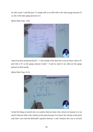
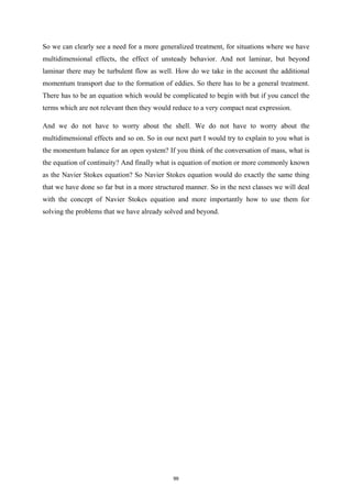
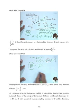
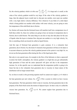
(Refer Slide Time 25:59)
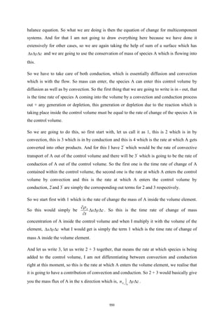
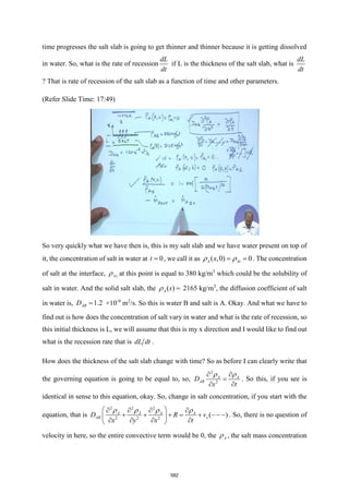
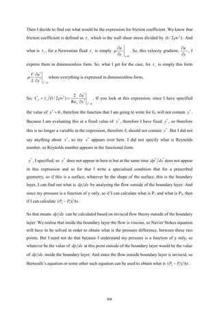
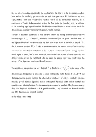
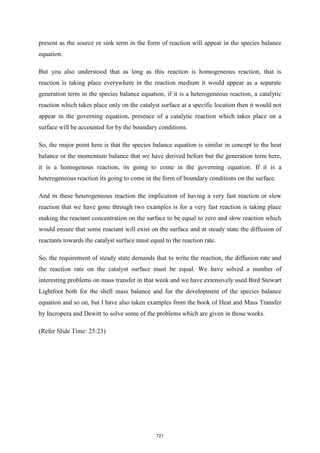
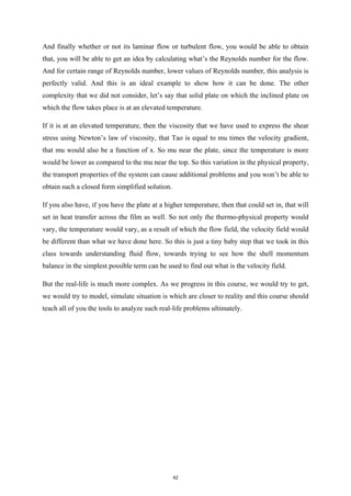
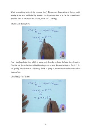
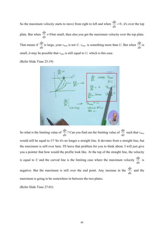
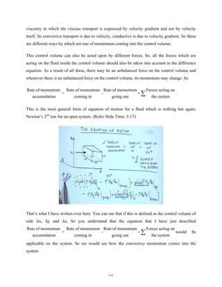
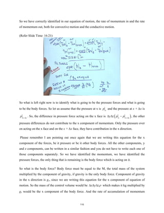
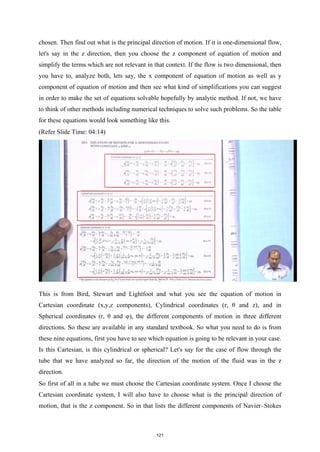
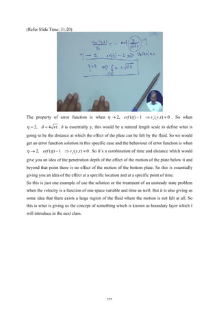
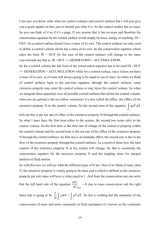
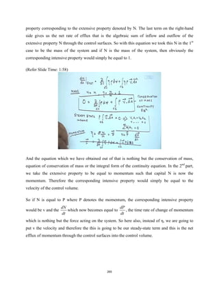
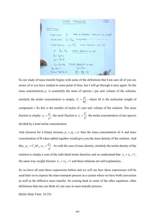
For 5
η = , the expression would become, [ ]
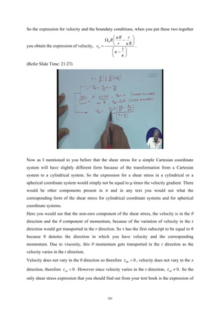
*
1
5 3.28324 0.34334
5
δ
δ
=− =
227](https://image.slidesharecdn.com/npteltpnotesfull-220501122717/85/NPTEL-TP-Notes-full-pdf-231-320.jpg)
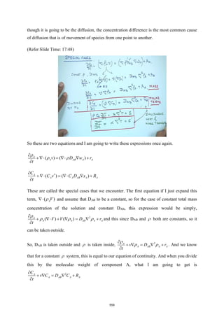
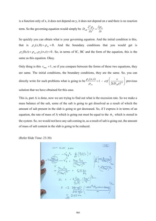
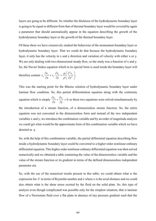
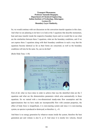
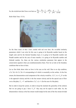
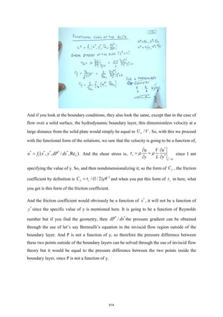
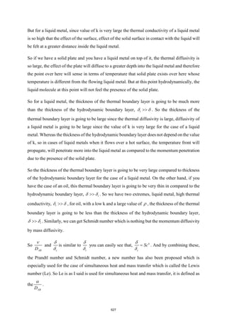
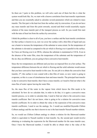
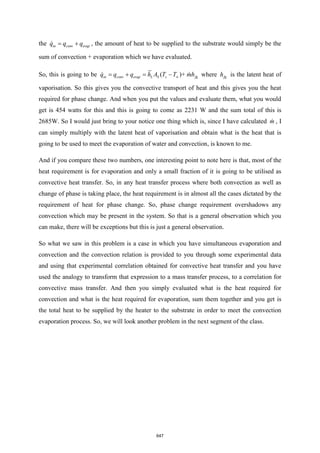
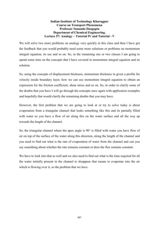
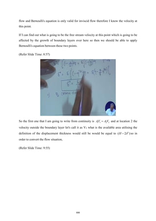
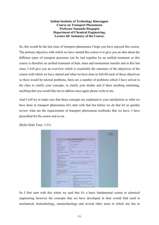
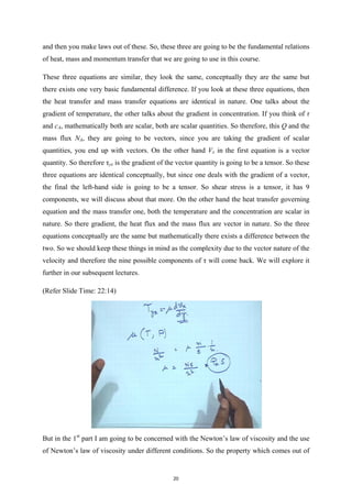
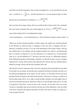
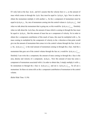
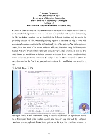
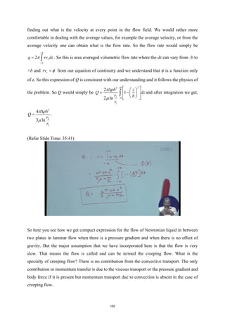
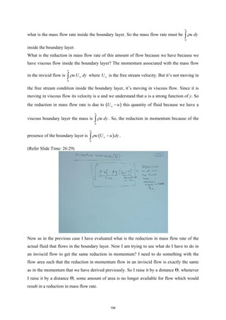
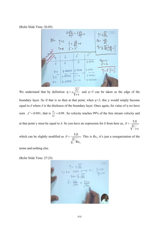
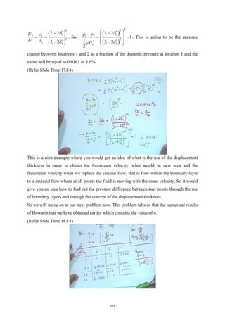
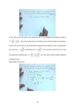
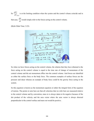
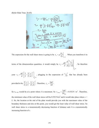
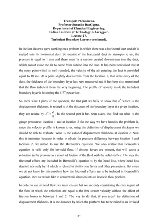
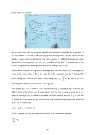
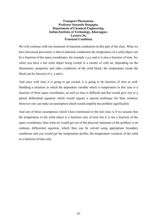
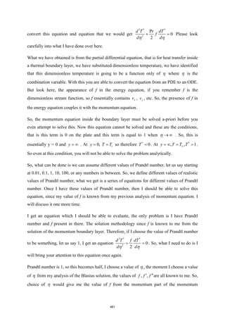
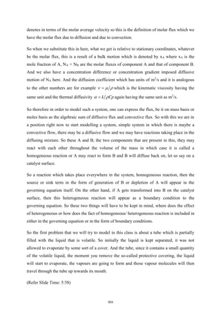
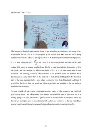
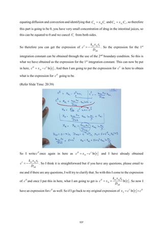
![*
δ
δ
at η=8 which is same as η → ∞ would be [ ]
*
1
8 6.27923 0.34415
5
δ
δ
=− = . So you can
compare these two values and can see that
* *
5
η η
δ δ
δ δ
= →∞
≈
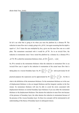
(Refer Slide Time 30:05)
So just the use of the table would give you some idea of how does displacement thickness
varies for different values of η, for different values of y and so on.
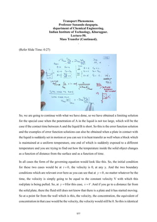
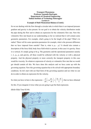
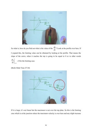
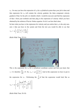
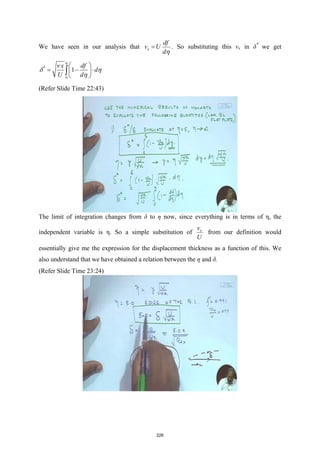
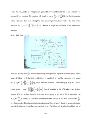
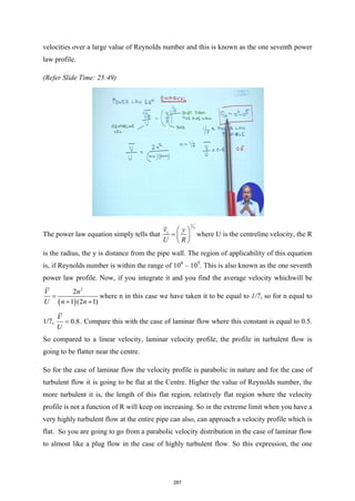
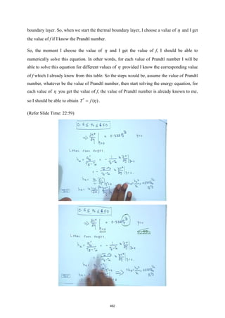
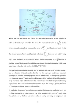
The next question that I posed to you to calculate the value of y
v
U
at the edge of the boundary
layer. I will write the expression for vy which we have derived before which is
1
2
y
U f
v f
x
ν
η
η
∂
= −
∂
. So y
v
U
would simply be
1
2
y
v f
f
U Ux
ν
η
η
∂
= −
∂
. This can be
expressed in terms of [ ]
1
2 Re
y
x
v
f f
U
η ′
= − .
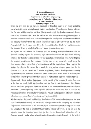
(Refer Slide Time 31:48)
229](https://image.slidesharecdn.com/npteltpnotesfull-220501122717/85/NPTEL-TP-Notes-full-pdf-233-320.jpg)
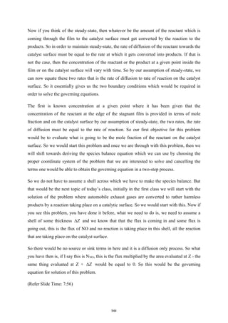
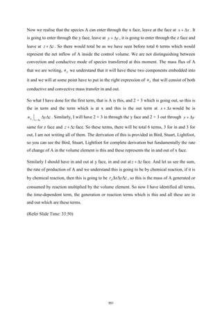
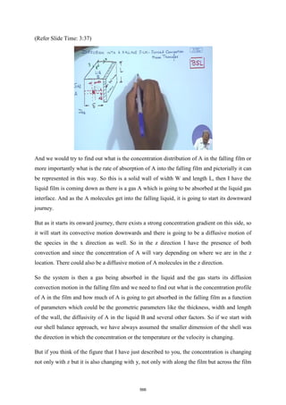
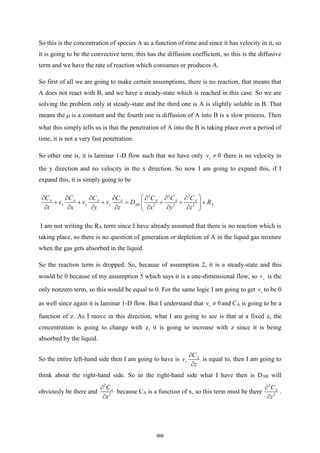
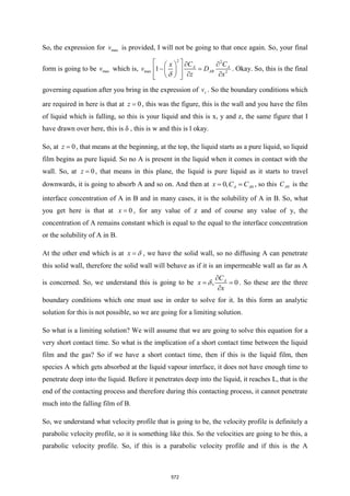
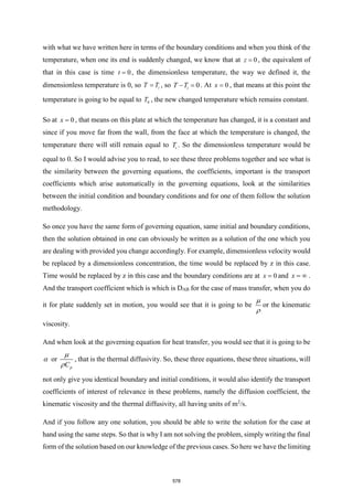
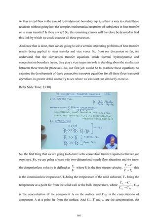
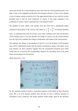
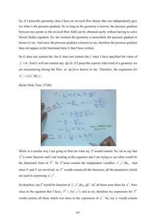
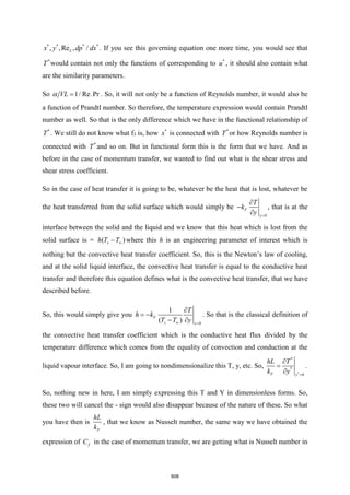
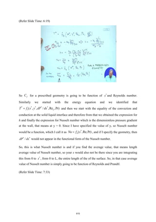
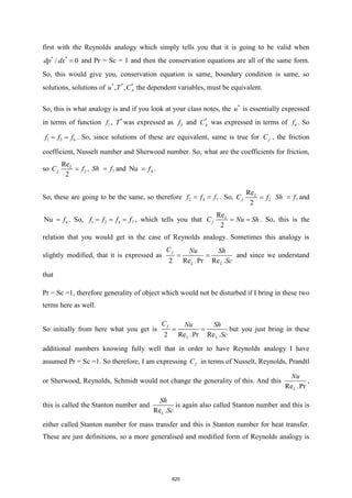
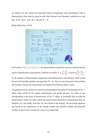
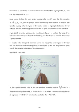
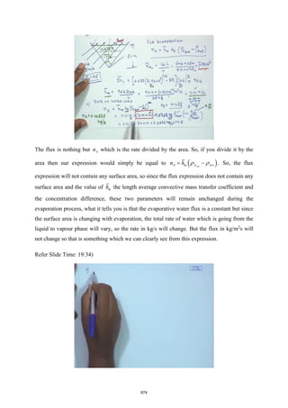
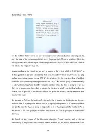
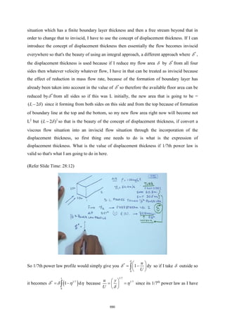
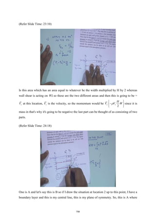
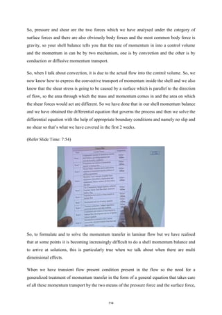
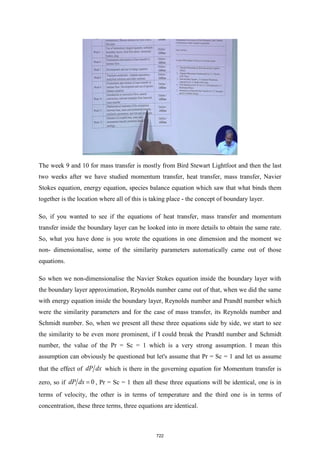
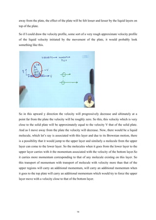
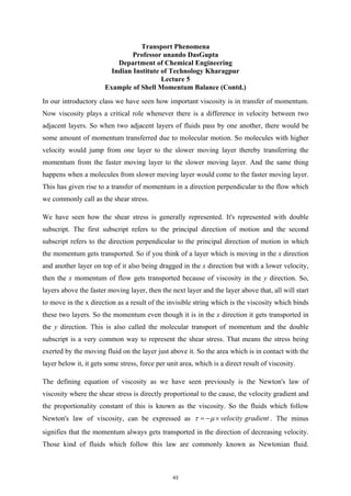
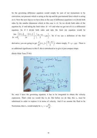
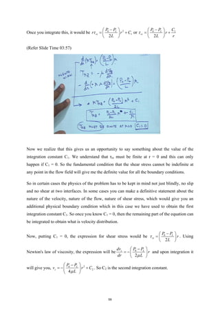
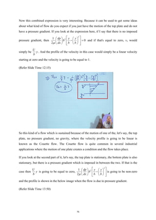
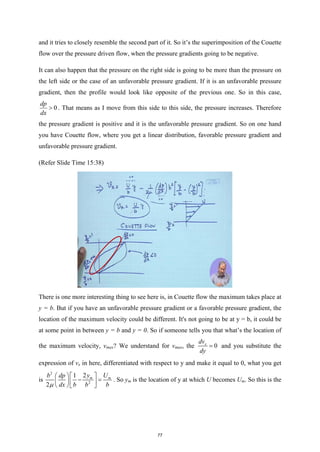
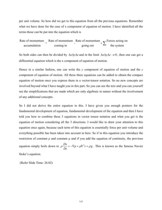
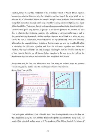
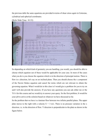
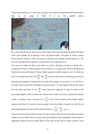
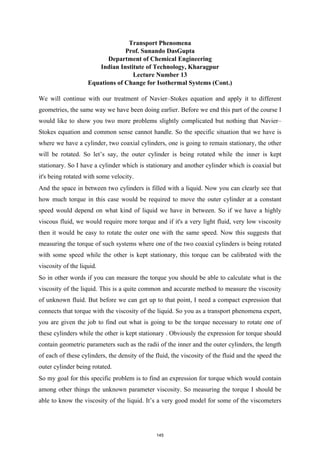
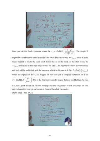
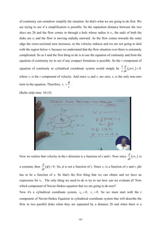
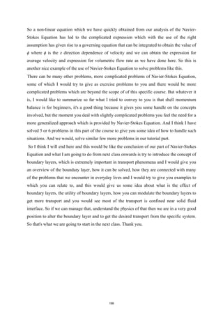
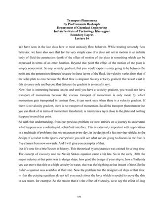
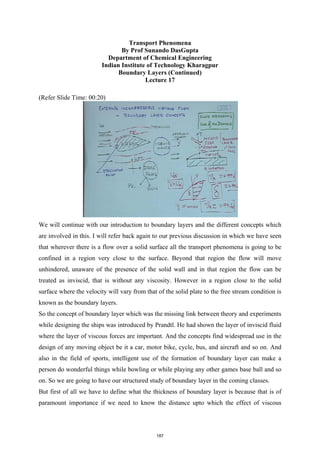
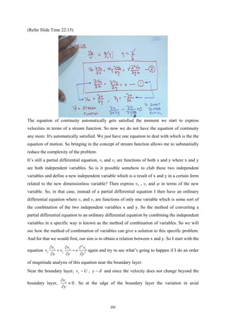
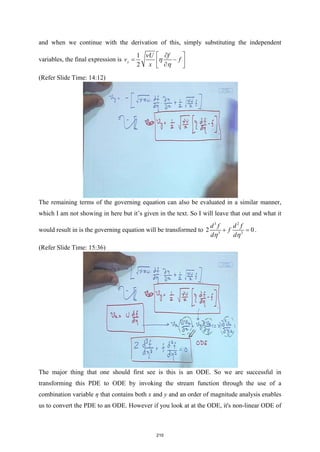
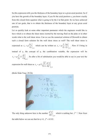
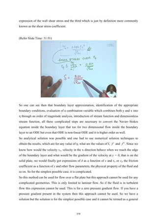
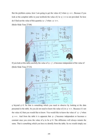
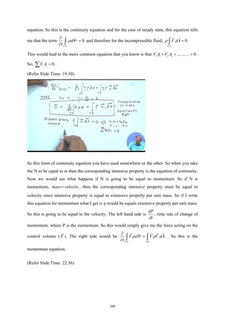
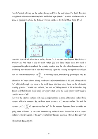
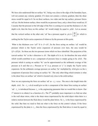
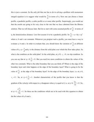
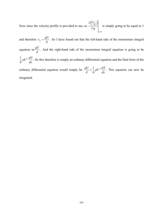
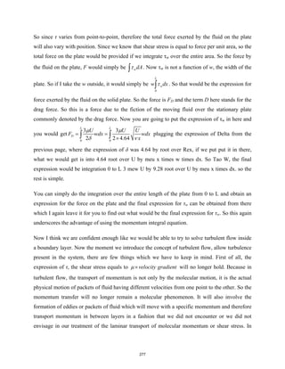
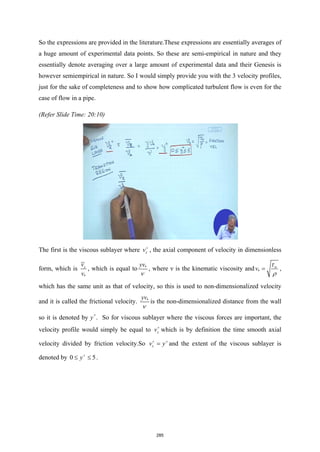
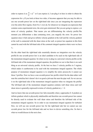
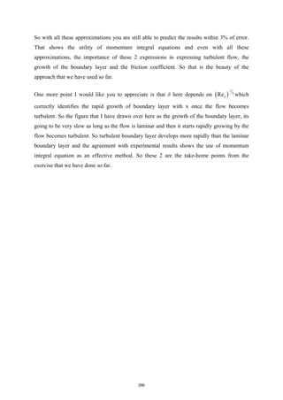
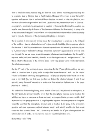
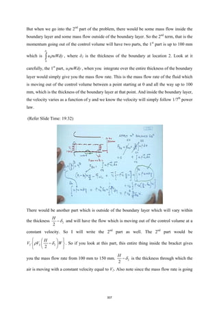
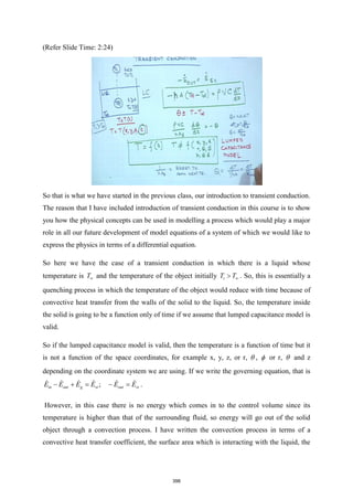
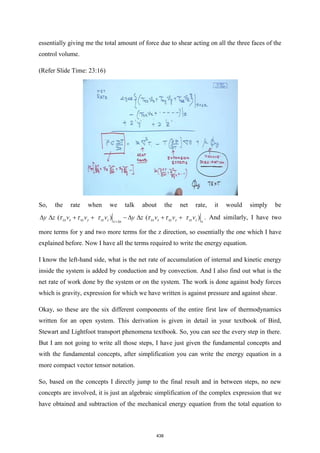
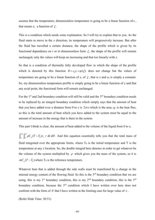
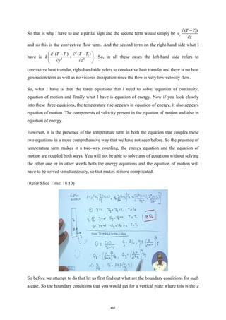
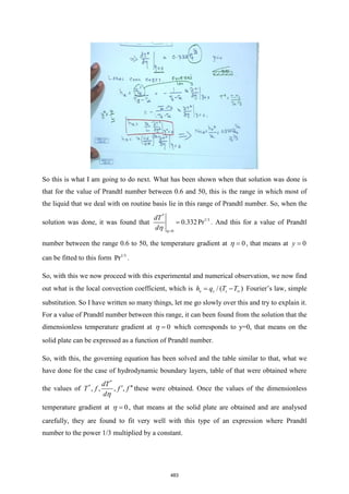
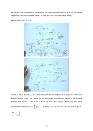
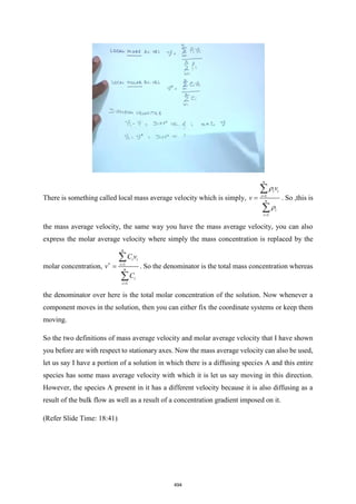
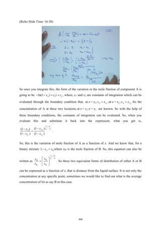
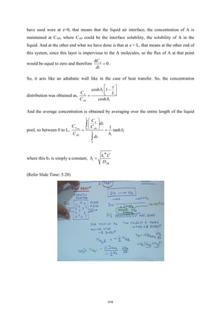
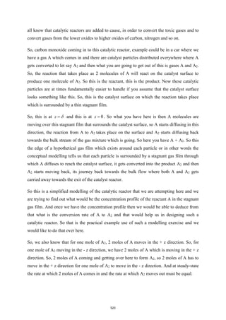
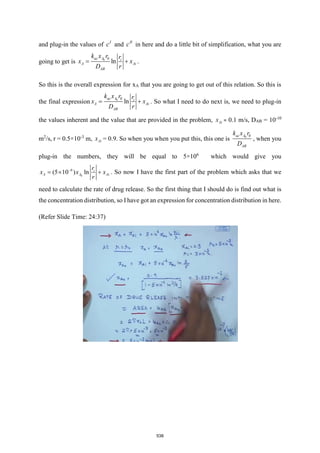
![So, at the edge of the boundary layer, that means at η=5,
[ ]
1
5 0.99155 3.28329
2 Re
y
x
v
U
= × − , this you get from the table. Therefore,
0.84
Re
y
x
v
U
= .
(Refer Slide Time 33:07)
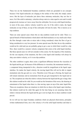
This gives me another insight into this boundary layer. On the solid surface you have vx and
vy both zero. You have vx inside the boundary layer and outside this vx is going to be equal to
U but what happens to vy in here? In other words can you call the edge of the boundary layer
as a streamline? Now in order for it to be streamline, it has to satisfy the basic properties of
the streamline which is that the particle which is on a streamline will remain on that
streamline and no particle, no fluid can cross a streamline. The moment you have flow across
a line, then that line cannot be a streamline. So you have yourself found out in the previous
problem that at the edge of the boundary layer, vy is not zero. vy is a function of Reynolds
230](https://image.slidesharecdn.com/npteltpnotesfull-220501122717/85/NPTEL-TP-Notes-full-pdf-234-320.jpg)
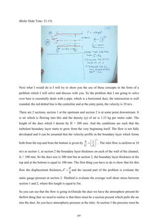
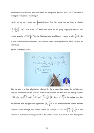
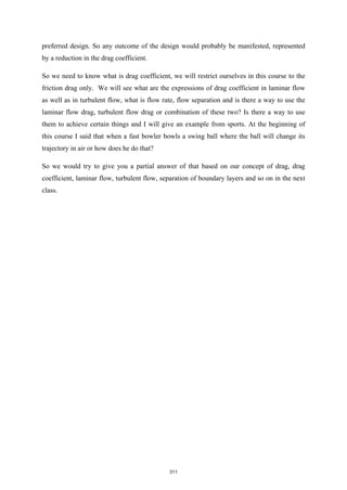
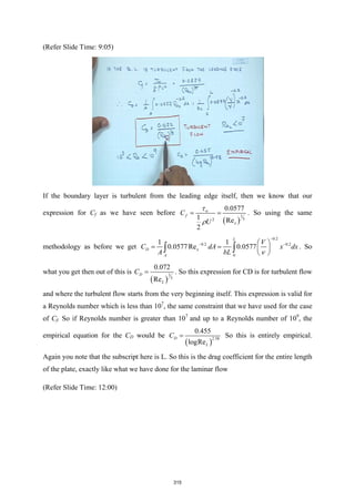
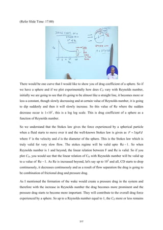
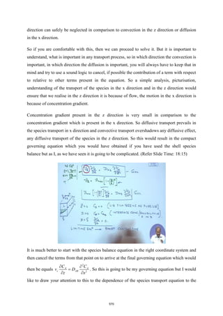
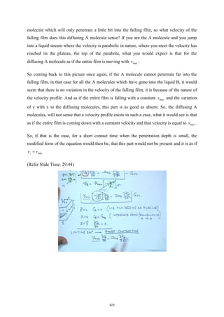
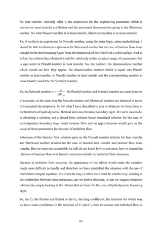
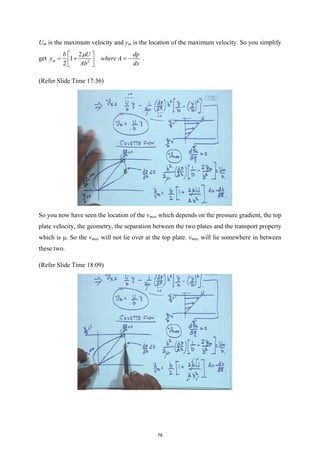
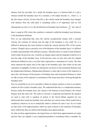
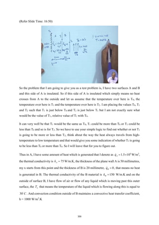
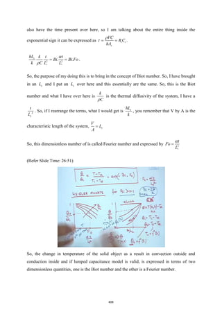
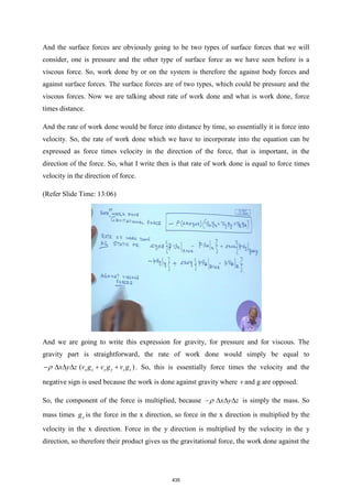
![end would give rise to significant pressure drag. In fact most of the drag that is experienced
by the moving spherical object in air is due to pressure drag.
It's the frictional drag constitutes only about 5 to 10%. But the situation gets reversed when
you go into turbulent boundary layer. The turbulent boundary layer, since the fluid molecules
carry more momentum with it, the point of separation on the sphere would start to move
backwards resulting in smaller wakes and smaller adverse pressure gradient. This is the
reason that turbulent boundary layer is often preferred over a blunt body. So for a blunt
object, we would rather have turbulent flow rather than laminar flow on a boundary layer.
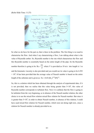
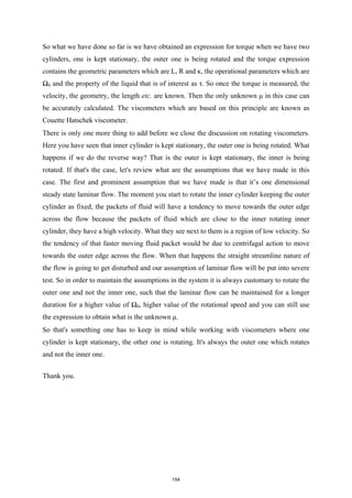
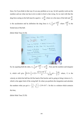
So the below figure of CD vs Re is a very well-known figure and of course for different
objects, the values of this CD would be different and its variation with Re would also be
different. But this roughly gives you an idea, starting at the Stokes regime, the laminar flow
and the turbulent flow, how CD changes, how wakes are formed, how wakes are reduced and
so on.
(Refer Slide Time: 26:16)
So if the red circle is a car, then the next car [the red rectangle] would like to be in the wake
formed by the first car and so on, such that it would have a pressure drag. So sometimes
intelligent use of the wake formed by the previous object would allow the object next to it in
a more intelligent fashion with less effort. So that is what we are going to explore further with
our example from cricket.
319](https://image.slidesharecdn.com/npteltpnotesfull-220501122717/85/NPTEL-TP-Notes-full-pdf-323-320.jpg)
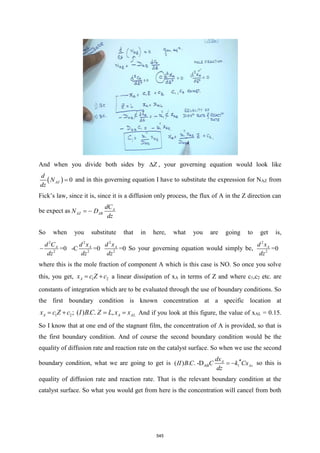
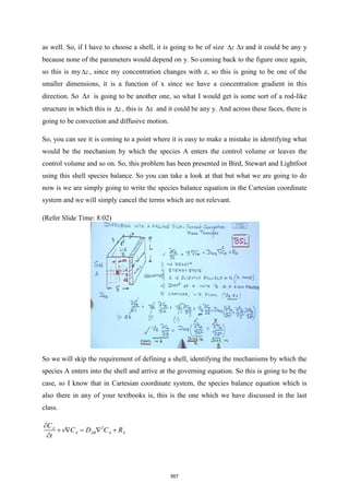
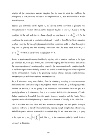
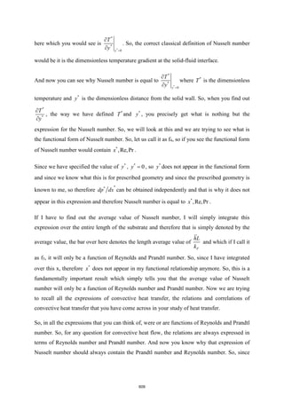
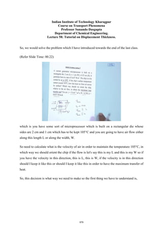
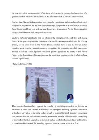
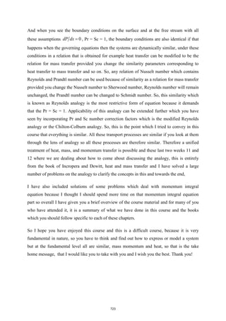
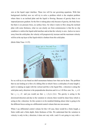
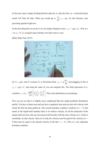
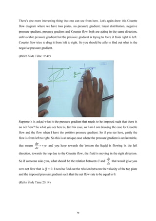
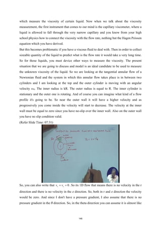
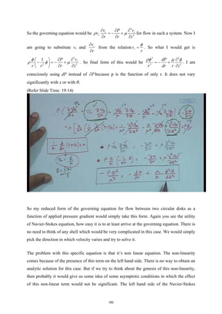
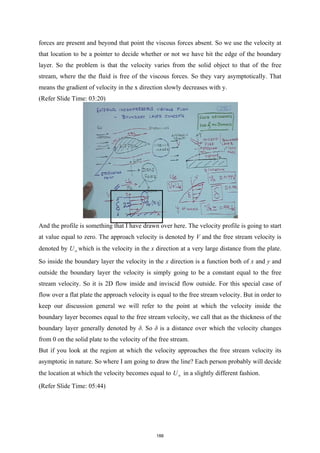
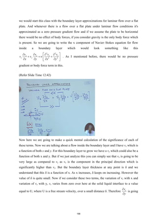
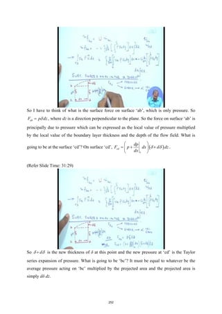
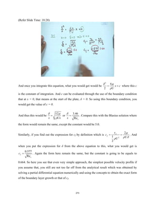
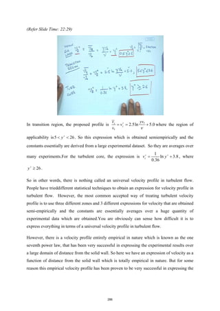
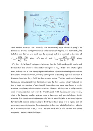
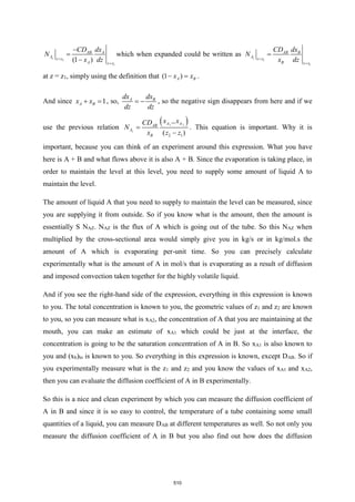
![Transport Phenomena
Prof. Sunando DasGupta
Department of Chemical Engineering
Indian Institute of Technology, Kharagpur
Lecture Number 30
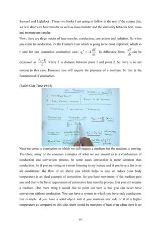
Heat Transfer Basics
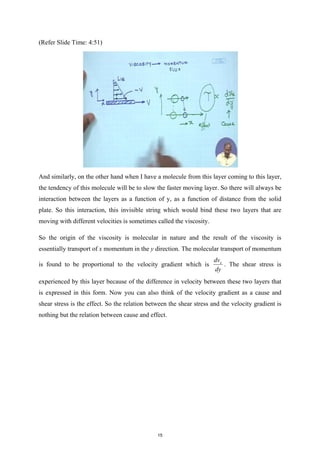
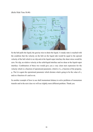
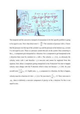
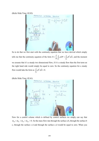
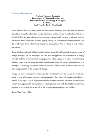
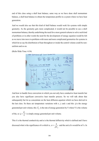
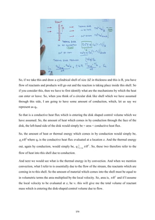
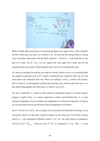
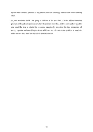
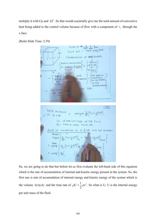
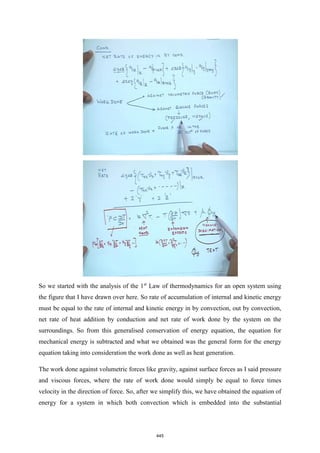
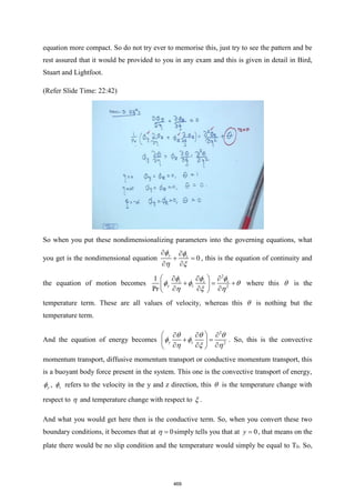
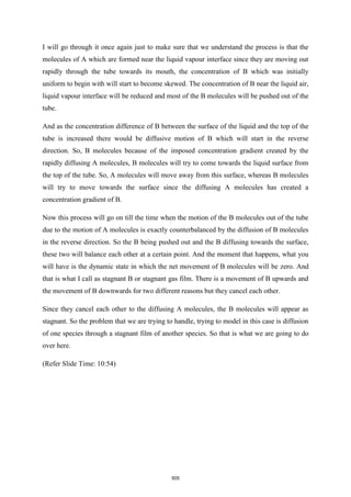
So far we have studied fluid mechanics, that is momentum transfer and details about the
boundary layers. What we saw is that the flow of momentum because of a difference in
velocity in between adjacent layers of fluid can be expressed in terms of Newton's law. So it's
the shear stress which also signifies the molecular transport of momentum, that was the basis
of our analysis of fluid motion. And there we have chosen initially a control volume and saw
what are the different methods, ways by which momentum is entering into the control
volume. So the rate of momentum coming into the control volume through convection as well
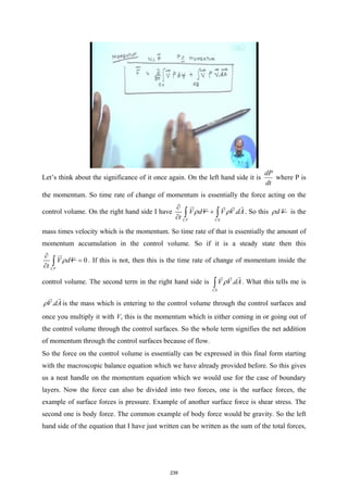
as molecular means which is conductive momentum transfer. So at steady state
rate of in - rate of out + sum of all forces = 0 and when I say all forces they can be body
force, for example gravity, or surface force acting on the control volume. If it is not at steady
state that means if all these contributions are not balanced then the control volume is going to
have an acceleration or deceleration of its own. So that was that was the starting point for the
derivation of Navier Stokes equation of motion of which Navier Stokes equation is a special
case where the viscosity and other properties are constant. So when we got to Navier Stokes
equation, [ ]
.
Dv
p g
Dt
ρ τ ρ
= −∇ − ∇ + , we saw that the left hand side of Navier Stokes equation
was
Dv
Dt
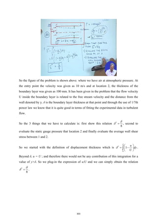
ρ which contains not only the transient effects, that means
v
t
∂
∂
, at the same time it
also has all the convective transport of momentum terms associated with it.
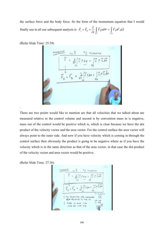
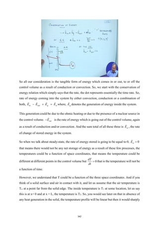
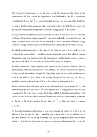
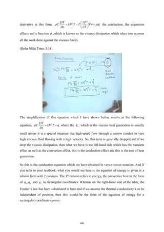
When we move to the right hand side of Navier–Stokes equation, we got a gradient in
pressure, p
−∇ , which is one of the surface forces, another term was due to viscous forces,
[ ]
.τ
− ∇ , and the third term that we got in Navier–Stokes equation was the effect of body
forces denoted by g
ρ where g is the acceleration due to gravity. So that was the equation of
motion which we have derived out of the simple consideration of Newton's second law for an
open system in which mass is allowed to come in with some velocity and go out as well. We
have seen examples of the use of Navier Stokes equation in different coordinate systems and
we saw how the use of Navier Stokes equation has simplified the overall treatment of fluid
mechanics leading to the accurate evaluation of the velocity in a flowing fluid.
332](https://image.slidesharecdn.com/npteltpnotesfull-220501122717/85/NPTEL-TP-Notes-full-pdf-336-320.jpg)
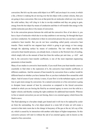
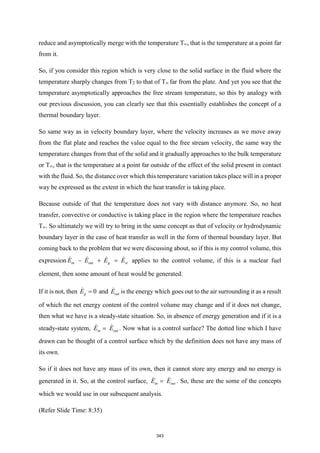
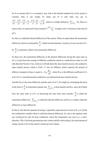
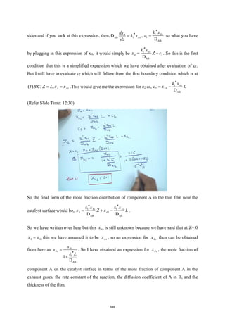
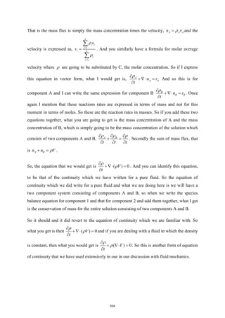
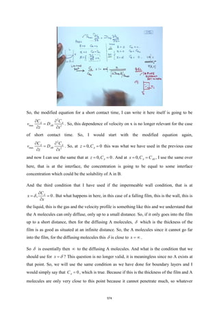
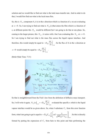
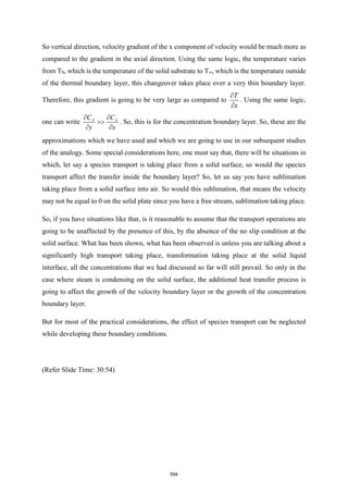
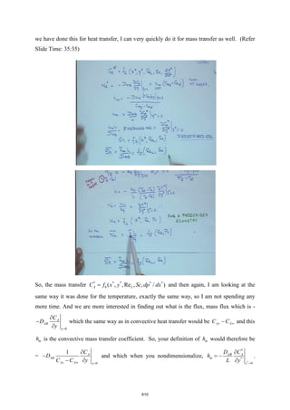
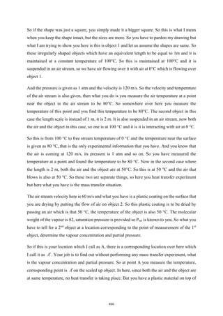
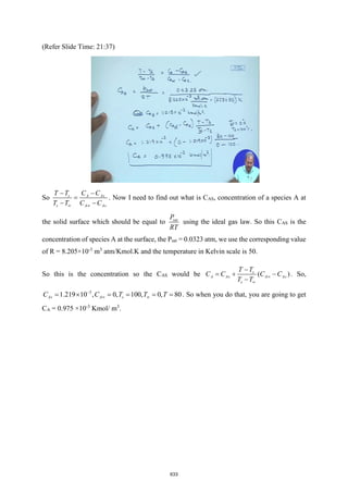
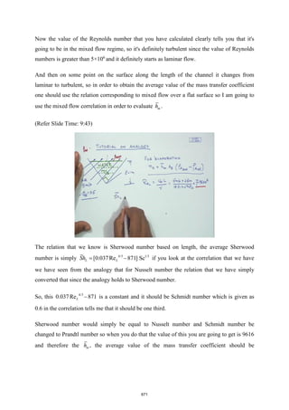
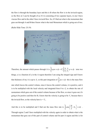
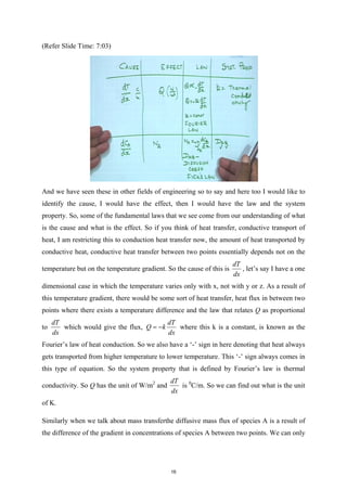
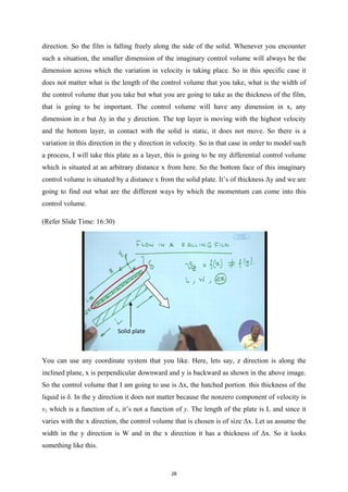
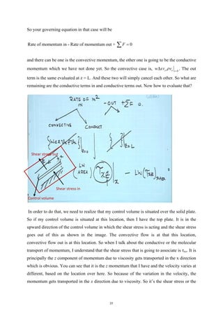
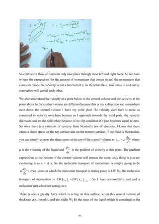
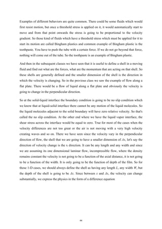
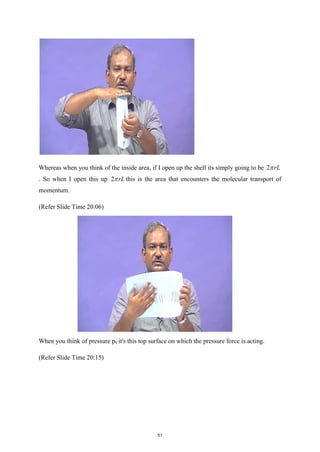
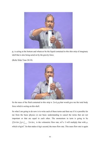
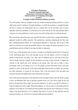
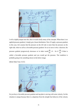
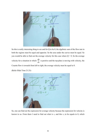
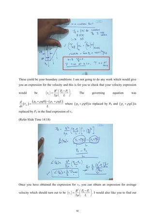
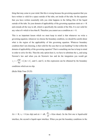
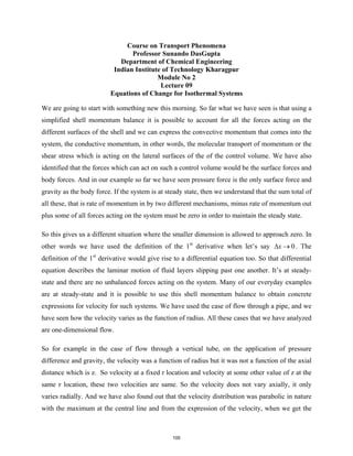
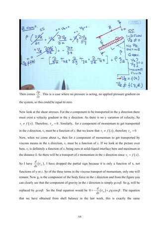
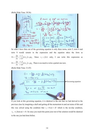
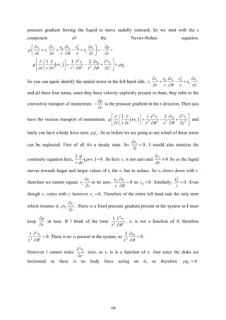
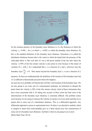
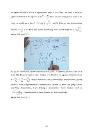
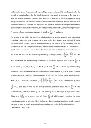
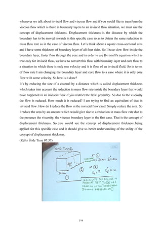
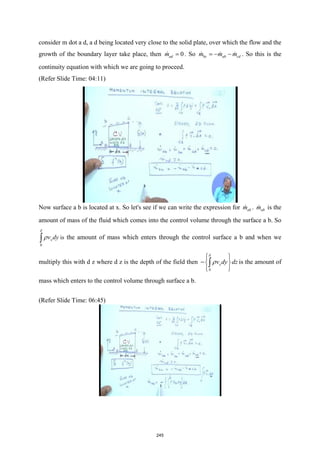
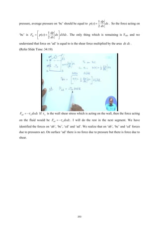
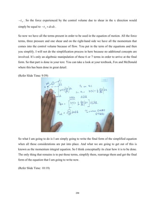
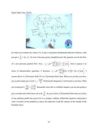
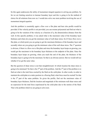
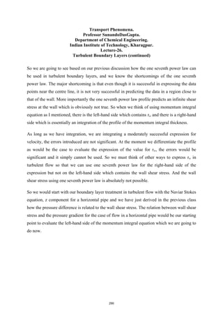
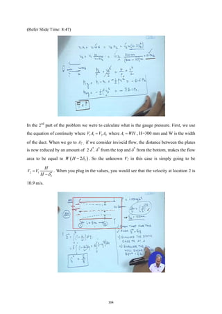
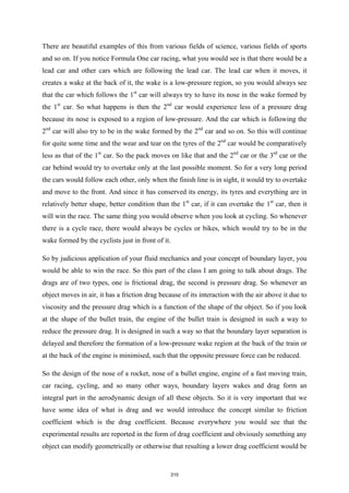
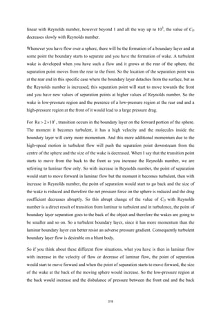
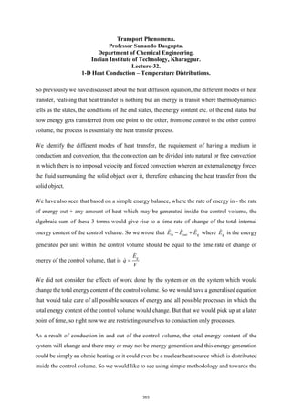
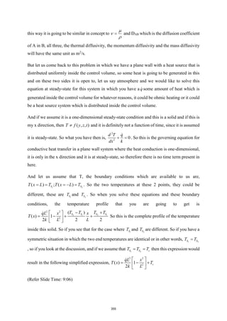
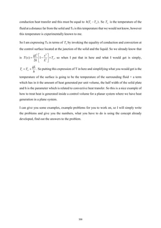
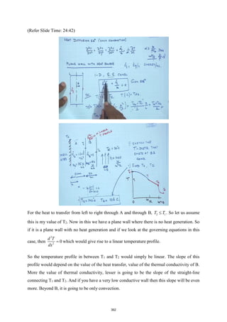
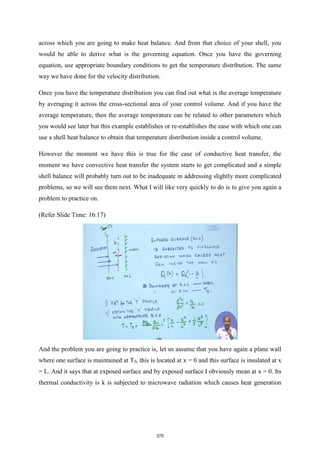
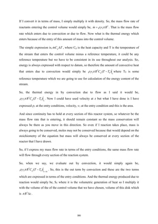
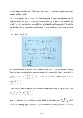
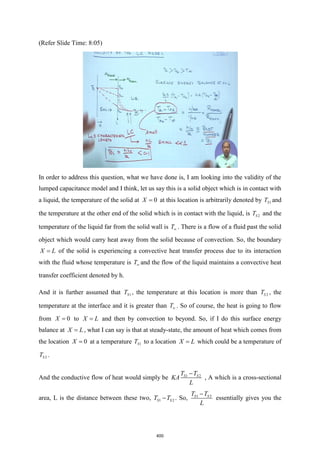
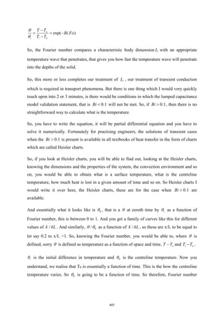
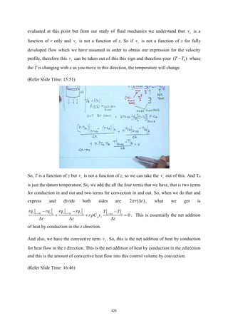
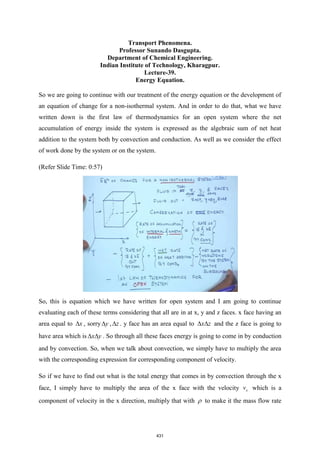
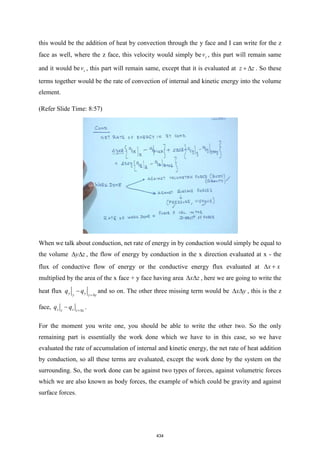
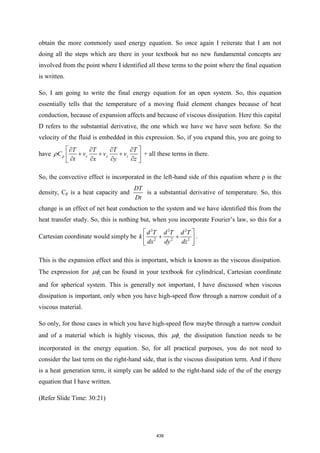
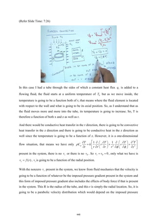
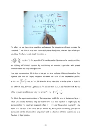
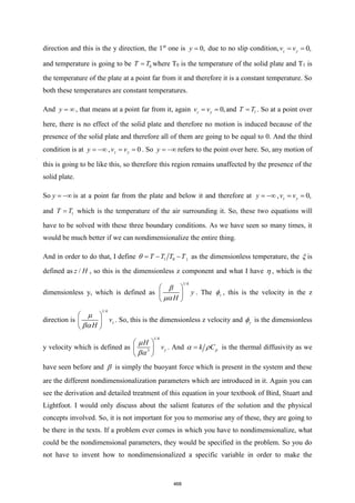
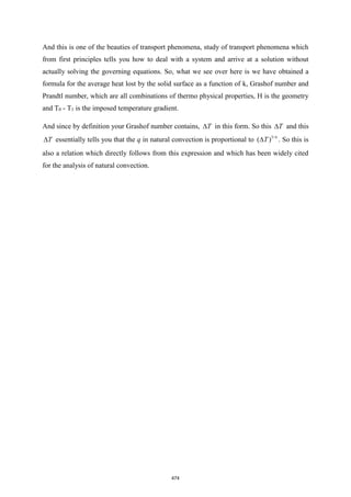
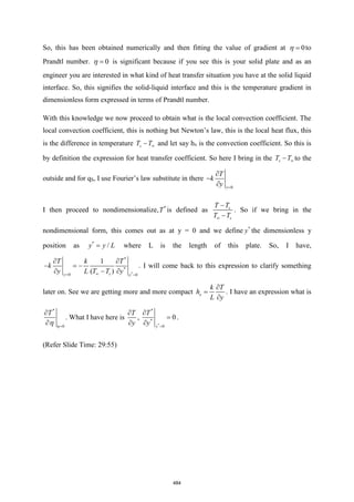
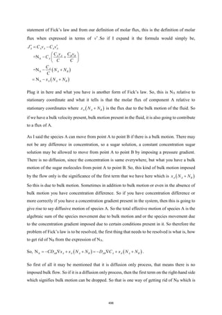
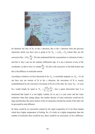
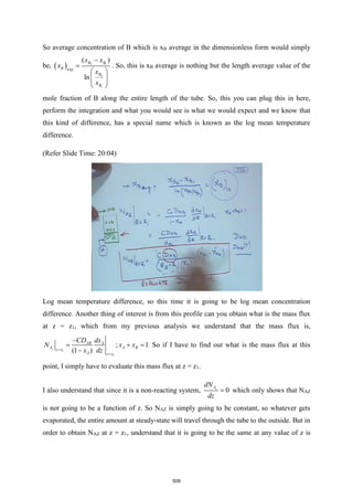
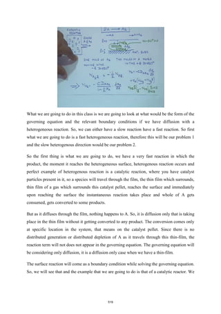
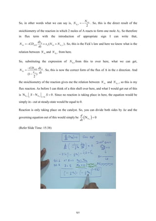
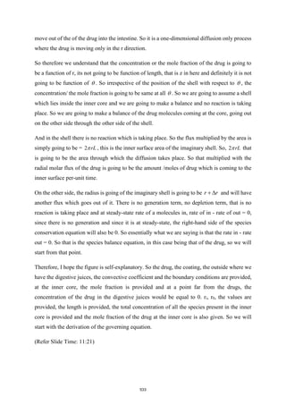
![(Refer Slide Time: 30:48)
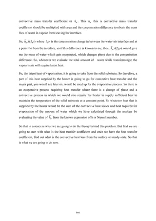
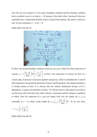
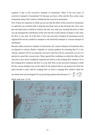
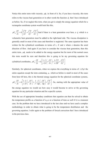
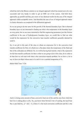
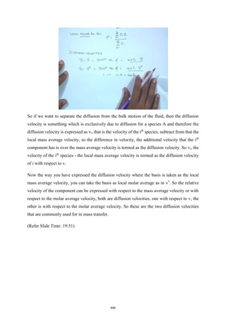
And the third condition could be that I have a convection surface condition where you have
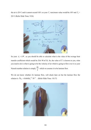
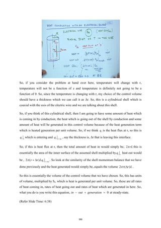
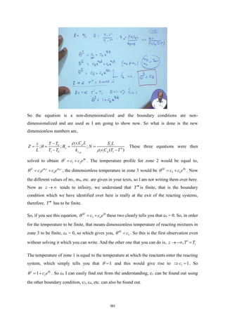
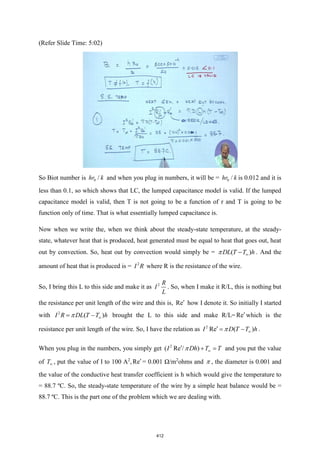
surface which is solid, on this side you have a liquid let’s say and the profile of temperature is
this where you have T , the temperature over here is T and the heat transfer coefficient
involved is h. So heat will come from here by means of conduction and from here to out by
means of convection.
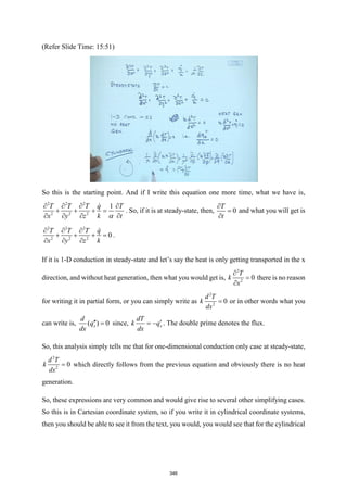
So what happens at steady-state is then
0
0
x
dT
k
dx =
− = , this essentially denotes the amount of
heat which comes in by conduction from the interior up to this point has to be equal to the heat
which goes out of the convection and if I use Newton’s law which would simply be
[ (0, ) ]
h T t T
− .
So, the convective heat loss must be equal to the convective heat which is coming to the
interface. So by conduction you have some amount of heat coming in and by convection the
same amount of heat is going out. So, this (0, )
T t denotes the temperature of the interface at
any given time at location x = 0 and T is the constant temperature of the bulk fluid situated far
from the solid wall. So, this is the convection surface condition.
So, we would use the conduction equation to start with the appropriate coordinate systems with
appropriate boundary conditions. And quickly try to solve and see if we can get the temperature
profile of a solid object which is experiencing conduction. Initially we would restrict ourselves
to the case of steady-state where the temperature could be a function of x, y, z or , ,
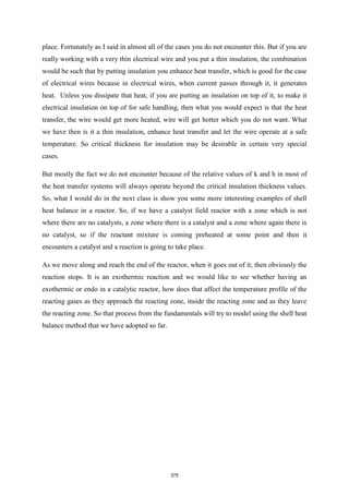
r z
or
351](https://image.slidesharecdn.com/npteltpnotesfull-220501122717/85/NPTEL-TP-Notes-full-pdf-355-320.jpg)
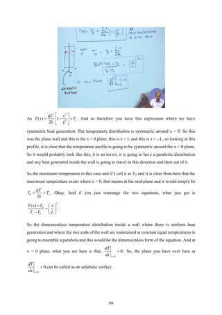
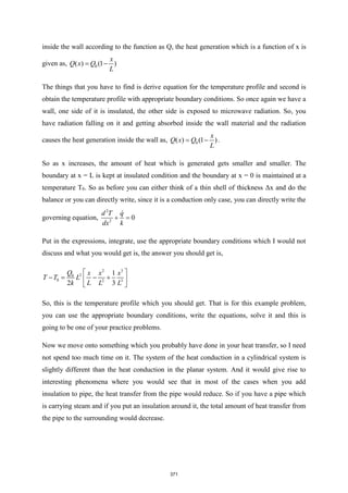

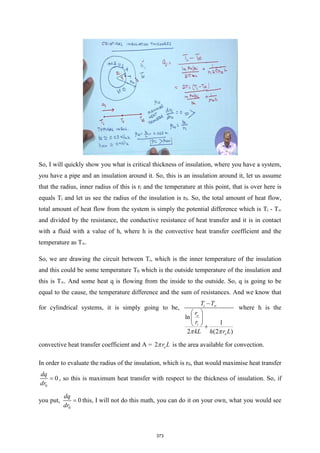
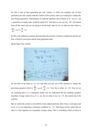
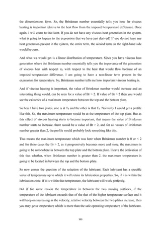
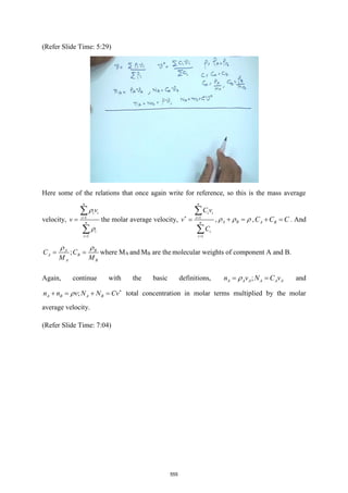
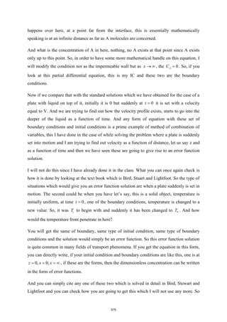
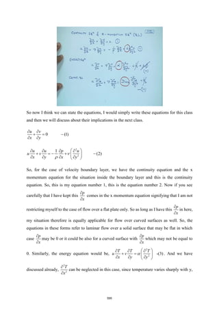
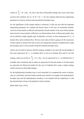
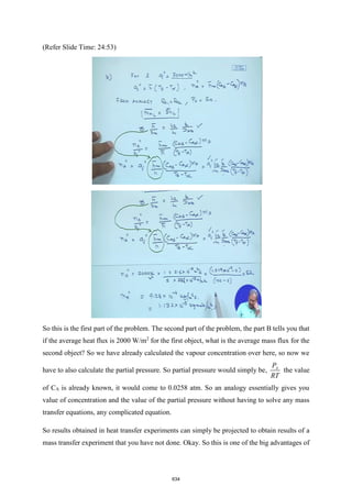
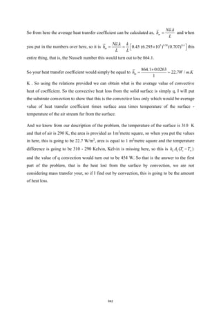
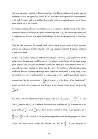
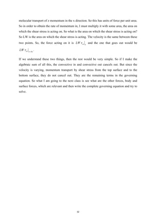
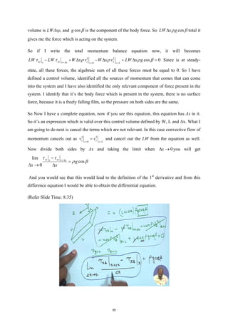
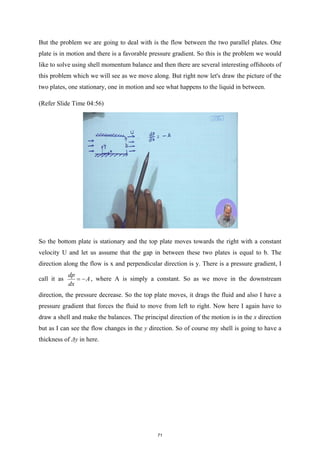
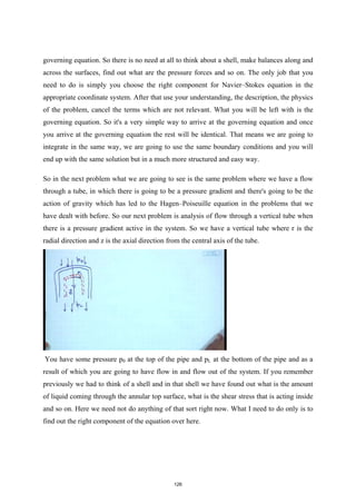
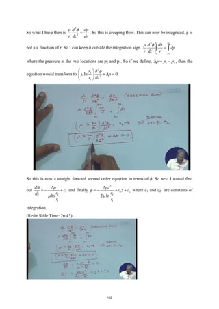
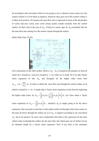
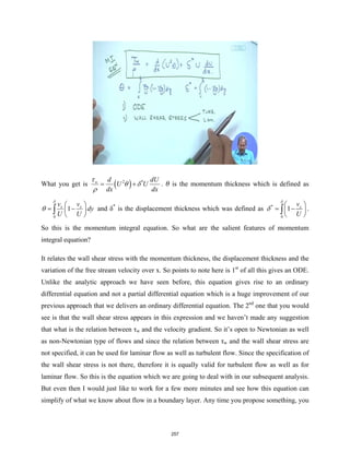
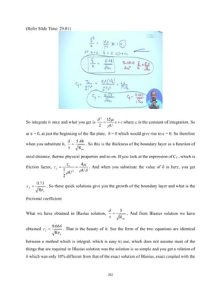
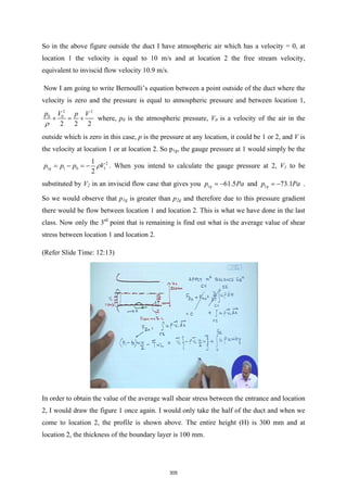
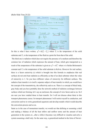
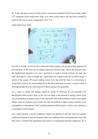
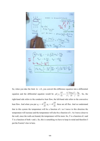
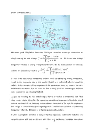
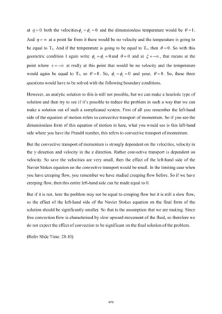
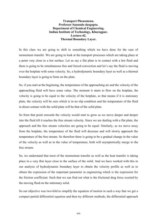
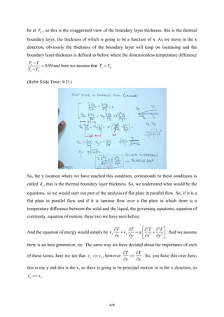
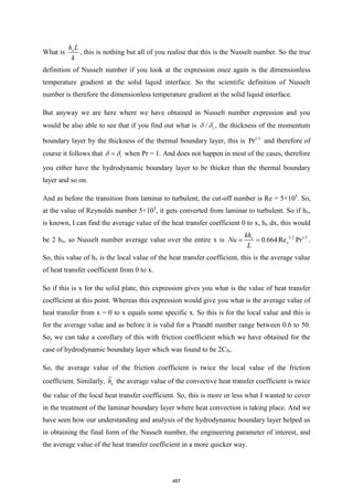
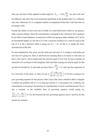
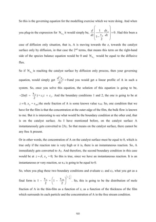
![expression. So, if you integrate this expression, what you would get is simply,
0
ln
exp[( ) ]
exp[( ) ]
i
t
s
s i
s
i
s
i i
VC d
dt
hA
VC
t
hA
hA
t
VC
hA
T T
t
T T VC
= −
= −
= −
−
= = −
−
And looking at, therefore the temperature of the object would change in exponential fashion
with time and the time constant of the process is simply the inverse of what I have written
inside the bracket.
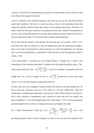
So, this is the convective heat transfer coefficient, this is the surface area, As, VC
. So, the
time constant of the process can be written as
1
s
VC
hA
. And as I mentioned before,
1
s
hA
is
the resistance due to conduction and VC
is some sort of thermal capacitance of the system.
So, the thermal constant of a process of quenching or of the process of changing the
temperature of a solid when it is exposed to a convection environment would be, this thermal
constant would depend upon the resistance to convection and the thermal capacity of the
system.
So, the behaviour of the variation of temperature with time is analogous to the voltage decay
that occurs when a capacitor is discharged through a resistor in an electrical circuit. So of
course, the higher the value of , the system will respond slowly in terms of the change in
temperature with time. But this gives you a very simple way to treat the transient conduction
in solid, provided you can use the lumped capacitance model.
So next we will quickly see how this constant, the that I have referred to in terms of s
hA
VC
how it can be combined to give you some more insight into the process. So, I am going to
start with the expression for which is s
hA
VC
. And therefore this can be written, this and I
405](https://image.slidesharecdn.com/npteltpnotesfull-220501122717/85/NPTEL-TP-Notes-full-pdf-409-320.jpg)
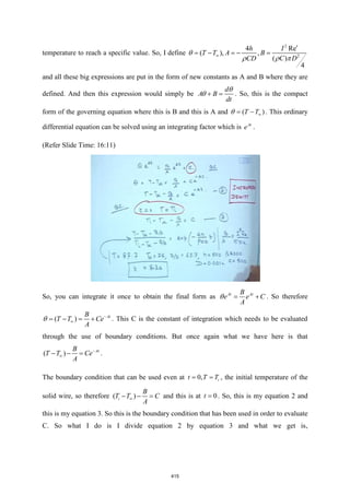
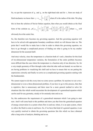
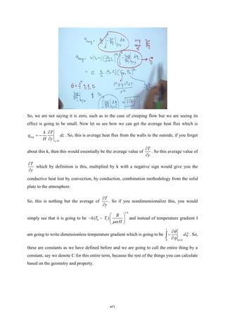
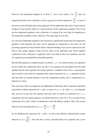
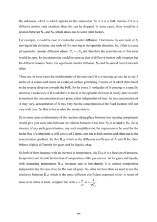
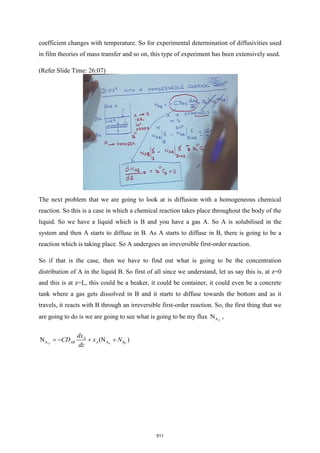
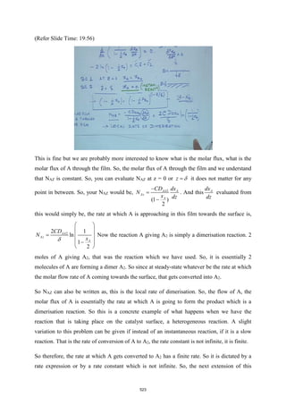
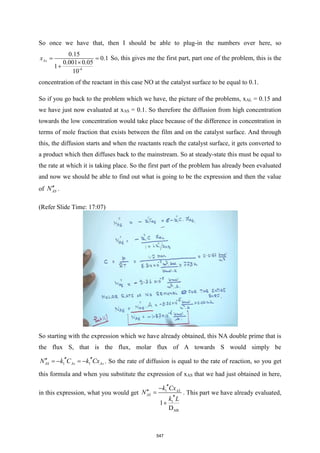
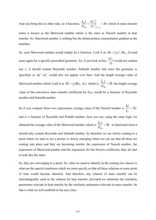
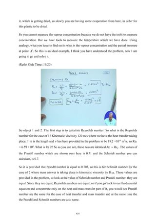
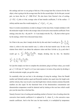
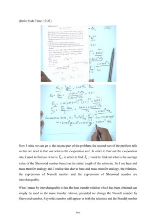
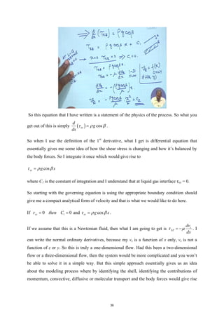
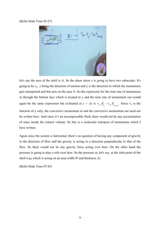
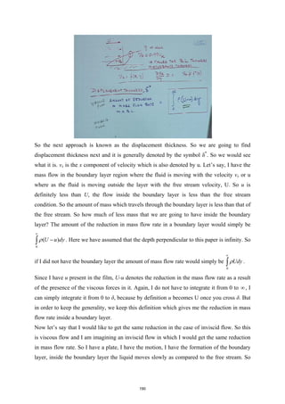
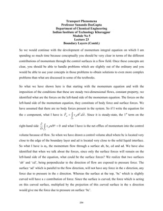
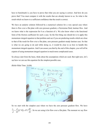
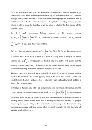
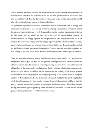
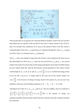
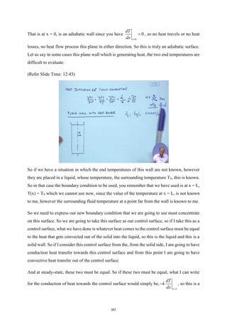
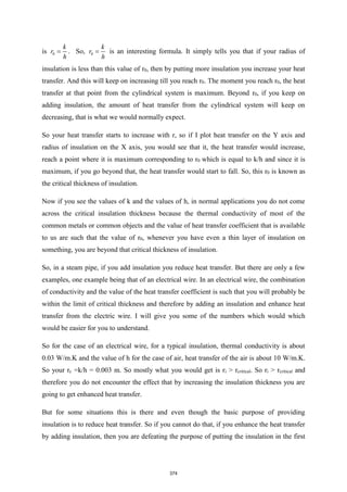
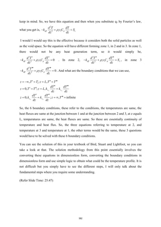
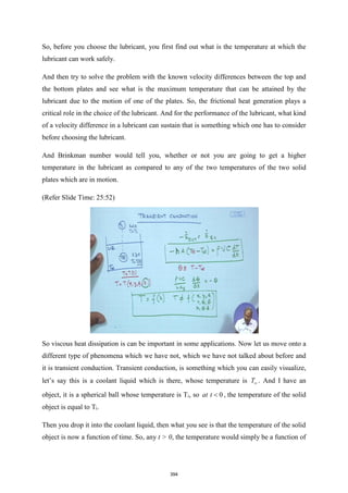
![I will write it once again that 0
6
(5 10 ) ln i
Ai
A
A x
r
x x
r
−
= + . Okay. So we realise that at 0
r r
=
that means at the outer edge of the inert coating, my 0
A
A
x x
= , let us call it at 0
A
x and we
understand that at Ai
x = 0.9, the value of 3
10
3
i
r −
= m and 3
0 0
5 1
r −
= m. So when you put
these values in here, what you are going to get is 0
A
x which is the mole fraction of component
A at the outside of the inert layer and is simply going to be 0
6 3
(5 10 ) ln
5
Ai A
A i
x x
x −
= +
So 0
A
x = 7
3.527 10−
. So it essentially tells the concentration of the drug on the outside is simply
going to be 7
3.527 10−
. The next that is remaining is rate of drug release which has been
asked, into the intestine that as a drug designer you must find out and we understand that since
I know 0
A
x , I should be able to multiply the convective movement of the drug away from the
outside of the inner core to the digestive juices.
So I am going to have this as 0
[ ]
ac A A t
area k x x C
− . So, ideally if you look at the total amount
of convection of the species away from the outer core of the inert material it is simply going to
be the convective mass transfer coefficient multiplied by the concentration difference. So that
when you multiply with the outer area of the inert coating it would give you in kg/s, in SI units,
what is the total amount of drugs that will diffuse through the inert layer, reach the outside of
the net layer and by a convection process initiated by the movement of the intestinal juices
inside the intestine that is going to get dissolved.
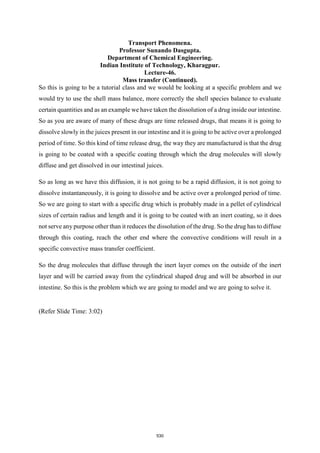
539](https://image.slidesharecdn.com/npteltpnotesfull-220501122717/85/NPTEL-TP-Notes-full-pdf-543-320.jpg)