Novel Navigation Strategy Study on Autonomous Mobile Robots

Peng Jia, Yumei Huang, Feng Gao & Yan Li
International Journal of Robotics and Automation (IJRA), Volume (1): Issue (4) 57
Novel Navigation Strategy Study on Autonomous Mobile Robots
Peng Jia pengjia_sdut@126.com
Ph.D Candidate/ School of Mechanical and
Precision Instrument Engineering,
Xi’an University of Technology
Xi’an, 710048, China College of
Computer Science and Technologe
Shandong University of Technology
Zibo, 255049, China
Yumei Huang hym_xaut@126.com
Faculty/School of Mechanical and Precision
Instrument Engineering, Xi’an
University of Technology
Xi’an, 710048, China
Feng Gao gf2713@xaut.edu.cn
Instrument Engineering,
Yan Li liyangf@xaut.edu.cn
Instrument Engineering,
Abstract
Potential field method has been widely used in obstacle avoidance for mobile
robots because of its elegance and simplicity. However, this method has inherent
drawbacks. Considering this, this paper introduces a new behaviour-based
navigation strategy. Aiming at a mobile robot SDLG-1 developed by the authors,
the kinematics model is built based on its motion structure. Using twelve sonar
sensors, the strategy algorithm of behaviour-based navigation control is brought
forth. Based on the algorithm, software simulations and experimental evaluations
have been conducted. Both results indicate the navigation strategy proposed in
this paper is effective.
Keywords: Behaviour-based navigation, mobile robot, kinematics model
1. INTRODUCTION
The task of navigation is to plan a path to a specified goal and to execute this plan, modifying it
as necessary to avoid unexpected obstacles. Intelligent navigation of mobile robot is one of the
challenging tasks among the researches and scientists throughout the world
[1]
. Potential field
method (PFM) for obstacle avoidance has become popular among researches in the filed of
robots and mobile robots. The idea of imaginary forces acting on a robot has been suggested by
Andrews and Khatib [2, 3]
. In the approach, obstacles exert repulsive forces onto the robot while
the target applies an attractive force to the robot. The sum of all forces determines the
subsequent orientation and speed of travel. The main reason for the popularity of PFM is its

simplicity and elegance. Simple PFM can be implemented quickly and initially provide acceptable
results without requiring many refinements [4]. In [5], the PFM is applied to off-line planning for
robot navigations. Literature [6] proposed a generalized PFM to combine global and local path
planning. The PFM has been implemented on mobile robots with real sensory data in [7, 8].
However, the mobile robot is very slow to avoid obstacles at 1.2mm/sec. In [9], a PFM called
virtual force field (VFF) has been developed. Based on the VFF experiment and research, four
defects of potential field method have been found: (1) trap situations exist due to local minima; (2)
no passage between closely spaced obstacles; (3) oscillations in the presence of obstacles; (4)
oscillation in narrow passages [4]. Although PFM has been updated in the following researches
[10-12]
, the four principle defects still possibly affect the final navigation results. Considering the
defects of potential field method, a behaviour-based navigation control algorithm is introduced in
this paper. Evaluations by software simulations have been successfully conducted on the indoor
autonomous mobile robot SDLG-1 developed by the authors.
2. KINEMATICS MODEL OF SDLG-1
2.1 Motion structure of the SDLG-1
The mobile robot SDLG-1 has two drive wheels and two passive wheels. Two-wheeled differential
drive system is applied in the design of the mobile robot SDLG-1 as shown in Figure 1. The
driving wheel system is composed of brushless DC servo motor, photoelectric rotary encoder,
hub of axle-coding wheel and hub of driving wheel. Relative positions of the robot can be realized
referring the photoelectric encoder and its wheel hub by the voyage method [13]
. The symbols
used in Figure 1 are listed and explained as follows.
ου is the center between the two drive wheels. l is the distance between the two drive wheels.
φ is the orientation angle at the time t . 1wV and 2wV is the independent rotational speed of the
left and right wheel, respectively. ovxV and ovyV is the speed of the center point ου in the
direction X ′and Y′, respectively. )(txov and )(tyov is the position of the mobile robot at time t.
)(tvω is the angular speed of the mobile robot at time t.
2.2 Kinematics model
In the global coordinate system {O, X, Y}, the constraints (pure rolling without slide) can be
expressed as:
0sincos =− φφ ovov xy && (1)
The kinematics model can be built:
















=










ov
ov
ov
ov
ov
w
v
y
x
10
0sin
0cos
φ
φ
φ&
&
&
(2)
The motion equation of the two-wheeled differential drive system is described as below:







−
=
−
=
l
VV
t
R
V
t
ww
v
w
v
12
1
)(
2
1
)(
ω
ω







−
+
=
−
=
12
21
12
.
2
)(
)(
ww
ww
ww
v
VV
VVl
tR
l
VV
tω




=
+==
0
).(
2
1)().( 12
ovy
wwvovx
V
VVtRtV ω
(3)
The position and orientation of the bodywork at a specific time can be indicated as:
(a) The developed SDLG-1
(b) Schematic diagram
FIGURE 1: The mobile robot SDLG-1










++=
++=
−
+=
∫
∫
∫
1
0
12
1
0
12
1
0
12
)(sin).(
2
1
)0()(
)(cos.)(
2
1
)0()(
)()(
)0()(
dttVVyty
dttVVxtx
dt
l
tVtV
t
wwovov
wwovov
ww
φ
φ
φφ
(4)
Where, )(tv and )(tω is the linear speed and angular speed at time t, respectively, )(tx and
)(ty are the position of the mobile robot at time t, which is represented by the center point ου
on the drive axle. φ is the included angle between the robot advancing direction and the X axis.
R is the turning radius.
In the control of the mobile robot, its expected motion status is tracked by working out )(tv and
)(tω using control arithmetic and the speeds of two driving wheels based on the above
equations. As can be known from the above motion equations, the motion system of the structure
cannot make abrupt changes in motion directions. The reason it that the system can only follow
the trajectory curve with continuous changes of the tangent angles when the two wheels make
same direction movements. The first order derivative of its motion curve must be continuous.
When the curve with the abrupt changes of the motion directions is being tracked, it is done by
making rotation of the mobile robot without advancing. The occurrence of such curves should be
avoided as far as possible in the path planning.
3. NAVIGATION CONTROL
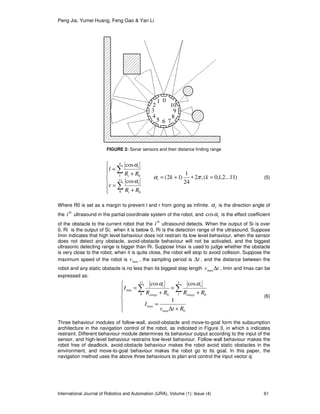
A sensor ring composed of twelve sensors is installed on the robot to get the information of
distance in every direction. Every sensor is used to detect the distance between the nearby
objects and the robot. As is indicated in Figure 2, “0” is the front end of the robot, “6” is the back
end, and the sectional drawings are the objects. What should be noted here is that the sonar
wave packet has a certain effective width and the distance information of the sensors is got by
calculating the wave packet which first reaches the surface of the object (the wave packet is not
necessary to reach the middle distance between the sensor and the obstacle)
[14-16]
. In Figure 2,
sonar sensor 0 and 11 has not received any echoes, so no precise calculation of the distance is
possible (for which, a margin can be set).
The twelve sonar sensors are indicated as Si (i=0, 1, …, 11). The output of Si is expressed as Ri.
When the angle of each sensor is set with respect to the current motion direction of the robot, the
existence of obstacles in every direction of the robot and the distance between the robot and the
obstacle can be determined. If Si does not detect any object in its corresponding direction, Ri = -
1; if Si detects an obstacle in the direction, Ri >0. l and r are used to indicate the approximate
extent of the obstacles on the right and left sides of the robot at its present position. When the
obstacle on the left is closer to the robot, it turns right; when the obstacle on the right is closer, it
turns left. The value of l and r can be determined as follows:

)11...2,1,0(,2
24
1
)12(
cos
cos
11
8 0
4
1 0
=∗+=







+
=
+
=
∑
∑
kk
RR
r
RR
l
i
i
i
i
i
πα
α
α
(5)
Where R0 is set as a margin to prevent l and r from going as infinite. iα is the direction angle of
the
th
i ultrasound in the partial coordinate system of the robot, and iαcos is the effect coefficient
of the obstacle to the current robot that the
th
i ultrasound detects. When the output of Si is over
0, Ri is the output of Si; when it is below 0, Ri is the detection range of the ultrasound. Suppose
Imin indicates that high level behaviour does not restrain its low level behaviour, when the sensor
does not detect any obstacle, avoid-obstacle behaviour will not be activated, and the biggest
ultrasonic detecting range is bigger than Ri. Suppose Imax is used to judge whether the obstacle
is very close to the robot, when it is quite close, the robot will stop to avoid collision. Suppose the
maximum speed of the robot is maxv , the sampling period is t∆ , and the distance between the
robot and any static obstacle is no less than its biggest step length tv ∆max , Imin and Imax can be
expressed as:







+∆
=
+
=
+
= ∑ ∑
0max
max
11
8
4
1 00
min
1
coscos
Rtv
I
RRRR
I
range
i
range
i αα
(6)
Three behaviour modules of follow-wall, avoid-obstacle and move-to-goal form the subsumption
architecture in the navigation control of the robot, as indicated in Figure 3, in which s indicates
restraint. Different behaviour module determines its behaviour output according to the input of the
sensor, and high-level behaviour restrains low-level behaviour. Follow-wall behaviour makes the
robot free of deadlock, avoid-obstacle behaviour makes the robot avoid static obstacles in the
environment, and move-to-goal behaviour makes the robot go to its goal. In this paper, the
navigation method uses the above three behaviours to plan and control the input vector q:
FIGURE 2: Sonar sensors and their distance finding range
01
2
3
4
5 6 7
8
9
10

3.1 Follow-wall Behaviour
After the behaviour is activated, the robot will move along the edge of the obstacle. The
conditions of activation (A) of the follow-wall behaviours are:
)002(
)002()(
108
42maxmax
>>−<
>>>>>
RR
RRIrIl
IIU
IIUI
πζ
πζ (7)
When the target point is in the first half cycle of the robot, and no obstacle exists in the direction
of S1 and S11, follow-wall behaviour will end. So the backout condition of the follow-wall
behaviour (B) is :
00]2,2[ 111 <<−∈ RR IIππζ (8)
Where, ζ is the angle between the current motion direction of the robot and the connecting line
between the robot and the target point, which can be calculated according to the difference
between the number of rolling circles of the right and left driving wheels, and the activation
condition and backout condition are boolean type variables, which is true when its value is 1. The
boolean type variables are defined as:



=
=
=
1,0
1,1
B
A
c (9)
where A and B is the activation condition and backout condition used in Equation (7),
respectively.
Thus, the effective condition of follow-wall behaviour is CAU .
3.2 Avoid-Obstacle Behaviour
The effective condition of avoid-obstacle behaviour is:
U U II
40 118
0)(
≤≤ ≤≤
>∪
i i
ii CARR (10)
The obstacle dead ahead of the robot has the biggest effect on it, so the output of avoid-obstacle
behaviour must satisfy the demand of avoiding the obstacle. Its control input is:








>∆−
≤∆
=
=
rlt
rlt
vtv
a
a
a
a
,/
,/
)(
0
0
0
max0
θ
θ
ω
(11)
where 0av and 0aω is the linear speed and rotary speed of the mobile robot for the next step,
respectively, maxv is the maximum linear speed, 0aθ is a set of values, indicating the orientation
of the robot in its one-step turn.
3.3 Move-to-Goal Behaviour
The effective condition of move-to-goal behaviour is:
Follow-wall
Move-to-goal
Avoid-obstacle
Actuator
s
s
FIGURE 3: SDLG-1 control structure

I II
40 118
1
≤≤ ≤≤
−=
i i
ii RR (12),
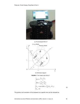
When the robot does not detect any obstacle, move-to-goal behaviour is activated. A polar
coordinate is established with the starting point S as the Pole point, X axis as the pole axis, as is
indicated in Figure 4, the current position of the robot R is:
πββρ 2)(0),(,( ≤≤ ttR (13)
The coordinate of the goal point D is:
πααρ 20),,( ≤≤D (14)
The distance between the current position and the goal point is RD and the expected turning
angle is )(tφ . Because of the limit of the maximum angular rate maxω , the planned control input of
move-to-goal behaviour is:




∆<∆
∆≥
=
tvRDtRD
tvRDv
tvmtg
max
maxmax
,/
,
)( (15)
where maxv is the maximum straight-line motion speed of the robot, and also:



≤
≥
=
max
maxmax
)(),(
)(,
)(
ωωω
ωωω
ω
ττ
τ
tt
t
tmtg (16)
Where, ttt ∆= /)()( γωτ







∈−
−−∈+
−∈+
∈
=
]3,2[)(,2)(
]2,3[)(,4)(
]0,2[)(,2)(
]2,0[)(),(
)(
ππδπδ
ππδπδ
πδπδ
πδδ
γ
tt
tt
tt
tt
t (17)
Where, )()()1()( ttt k
θαψδ −+−=



∪−∈−
−∪∈−
=
]2,[]0,[)(,1
],2[],0[)(,0
πππβα
πππβα
t
t
k (18)
FIGURE 4: Polar coordinate of the move-to-goal behaviour

)(cos2
)(cos
arccos)(
22
t
t
t
RDRD
RD
ηρρρρ
ηρρ
ψ
−+
−
= (19)







−−∈−+−
∈−+−
∈−−
∈−−
=
],2[)(,2)(
]2,[)(,2)(
]0,[)(,)(
],0[)(),(
)(
ππβαπβα
ππβαπαβ
πβααβ
πβαβα
η
tt
tt
tt
tt
t (19)
According to the above equations, the robot can plan a relatively good path without collision in
complicated environment. The above-discussed three navigation behaviours have good stability.
4. SIMULATION EVALUATION
Experiment I: The environment of obstacle avoidance simulation experiment is a section of
corridor in the simulation lab environment, as is shown in Figure 5, where the red colour shows
the walls and the blue colour shows the obstacles. A distance of 8 meters is set between the
starting point S and the object point G and 4 static obstacles are placed between the two points.
The corridor is 3 meters wide. The width of obstacles 1 and 2 is 0.3 meter. The horizontal
distance between obstacle 1 and 2 is 1.2 meters. The distance between obstacle 2 and 3 is 0.8
meter. The distance between obstacle 3 and 4 is 0.9 meter. Obstacle 3 is an irregular object, and
obstacle 4 is a ball with a diameter of 0.7 meter. The diameter of the robot is 0.45 meter.
The robot first entered into the follow-wall behaviour. When it reached the point P1, it detected
obstacle 1. Because the wall and obstacle 1 form a turn, the robot will sway from side to side and
enter into the “canyon effect”, one of the possible solutions is to add states in programmes so that
the robot can use them to memorize the action that it is taking at present and consequently to
prevent itself from making opposite operation to make itself sway from side to side. Then it
continued its follow-way behaviour. It made forward-right movement to evade obstacle 1. When it
reached the point of P2, navigation behaviour was activated again. Between the position of P2
and the position of P3, the follow-wall behaviour and made by the robot switched frequently.
When the robot detected obstacle 3 and obstacle 4, the obstacle avoidance behaviour was
activated, and finally it reached object G. Figure 5 shows the simulated path of the mobile robot.
The simulation results show this behaviour-based navigation can activate corresponding
behaviours according to the environment. The three behaviours collaborate each other closely
and consequently avoid the four drawbacks by using the PFM. So the behaviour-based
navigation introduced in this paper is more concise and more convenient for realization than that
of PFM.
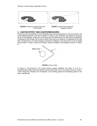
Experiment II: In the experimental fied with traps, the robot navigated by traditional potential field
method cannot escape from the traps as shown in Fig. 6. As shown in Fig. 7, by the new
navigation method, the robot escapes from the trap quickly. The robot can escape from the trap
clockwisely or counterclockwisely denpending on the programming parameters. Further hardware
and software realization are needed for the automatic direction selection to realize the shortest
moving path.
G
3
S 1
2P1
P2
P3
4
FIGURE 5: Simulation of the autonomous obstacle avoidance

FIGURE 6: Results by traditional potential FIGURE 7: Results by the proposed
Field method navigation method
5. CANYON EFFECT AND COUNTERMEASURES
If there are a lot of obstacles or some obstacles have concave geometries in the environment, the
avoid-obstacle behaviour may fail. As shown in Figure 8, such mistakes may happen at the sharp
corner of the obstacle. Under such circumferences, the robot will turn to right due to the detection
of obstacle at the left side. But it will turn back to left due to the detection of obstacles at the right
side. Consequently, the robot changes its directions endlessly. This phenomena is the so-called
canyon effect. In order to avoid such effects, states are added to the strategy as shown in Figure
9.
In Figure 9, Text-timer(X) is the timing function always feedback true state. X is R or L
representing the right or left drive wheel. Function Start-timer (X,T) is to create a timer for X and T
is the timing time. Rotation and Translation is the rotating speed and translating speed of the
robot, respectively.
FIGURE 8: Canyon effect
Mobile robot

6. EXPERIMENTAL EVALUATIONS
Based on the coordinate setting as shown in Figure 1, the position of point O’ under coordinate
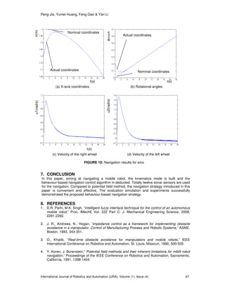
ΣO is represented by the vector P=[x y Ф]T. Ф is the orientation of the mobile robot.Given the arc
path as: x=2cos(Ф), y=2sin(Ф), and Ф=0.03t, based on the navigation strategy mentioned above,
the experimental results are shown in Figure 10.
From Figure 10 and Figure 11, the mobile robot SDLG-1 has realized navigations fro expected
paths, which validated the navigation strategies introduced in the paper.
FIGURE 9: Diagram for eliminating the canyon effects
Y
Rotation=-ω
Translation=0
N
Text-timer(R)=true?
Rotation= ω
Translation=0
Y
N
L=true?
Start-timer（L,T）
Y
N
R=true?
Y
Start-timer（R,T）
Rotation=-0
Translation=c
N

7. CONCLUSION
In this paper, aiming at navigating a mobile robot, the kinematics mode is built and the
behaviour-based navigation control algorithm in deducted. Totally twelve sonar sensors are used
for the navigation. Compared to potential field method, the navigation strategy introduced in this
paper is convenient and effective. The evaluation simulation and experiments successfully
demonstrated the proposed behaviour-based navigation strategy.
8. REFERENCES
1. D.R. Parhi, M.K. Singh, “Intelligent fuzzy interface technique for the control of an autonomous
mobile robot,” Proc. IMechE Vol. 222 Part C: J. Mechanical Engineering Science, 2008,
2281-2292.
2. J. R., Andrews, N., Hogan, ‘Impedance control as a framework for implementing obstacle
avoidance in a manipulator, Control of Manufacturing Process and Robotic Systems,” ASME,
Boston, 1983, 343-351.
3. O., Khatib, “Real-time obstacle avoidance for manipulators and mobile robots,” IEEE
International Conference on Robotics and Automation, St. Louis, Missouri, 1990, 500-505.
4. Y. Koren, J. Borenstein,” Potential field methods and their inherent limitations for mibilt robot
navigation,” Proceedings of the IEEE Conference on Robotics and Automation, Sacramento,
California, 1991, 1398-1404.
x(m)
Ф(rad)
(a) X-axis coordinates
FIGURE 10: Navigation results for arcs
t(s) t(s)
(b) Rotational angles
Actual coordinates
Nominal coordinates
Actual coordinates
Nominal coordinates
(c) Velocity of the right wheel
u1(rad/s)
u2(rad/s)
(d) Velocity of the left wheel
t(s)

5. C. Thorpe, A. Stentz, S. Shafer, “An architecture for autonomous vehicle navigation,”
Computers in Aerospace Conference, 5th Long Beack, CA, 1985, 22-27
6. B.H. Krogh, C. Thorpe, “Integrated path planning and dynamics steering control for
autonomous vehicles,” Proceedings of the 1986 IEEE International Conference on Robotics
and Automation, SFO, California, 1986, 1664-1669.
7. R.A. Brooks, “A robust layered control system for a mobile robot,” IEEE Journal of Robotics
and Automation, Vlo.RA-2, 1986, 14-23.
8. R.C. Arkin, “Motor schema-based mobile robot navigation”, The International Journal of
Robotics Research, 1989, 92-112.
9. J. Borenstein, Y. Koren, “Real-time obstacle avoidance for fast mobile robots”, IEEE
Transactions on Systems, Man, and Cybernetics, 1989, 1179-1187.
10. P. Coelho, U. Nunes, “Path-following control of mobile robots in presence of
uncertainties,”IEEE Transactions Robotics, 2005, 21:252-261.
11. G. Antonelli, S. Chiaverini, G. Fusco, “A calibration method for odometry of mobile robots
based on the least-squares technique”: Theory and experimental validation, 2005, 21:994-
1004.
12. J.M.M. Tur, J.L. Gordillo, C.A. Borja, A closed-form expression for the uncertainty in odometry
position estimate of an autonomous vehicle, IEEE Transactions on Robotics, 2005, Vol. 21,
1017-1022.
13. Joseph L. Jones, Daniel Roth,” Robot programming: a Practical Guide to Behaviour-Based
Robotics”, 2004, McGraw-Hill.
14. Hongbo Wang and takakazu Ishimatsu, “Vision-based Navigation for an Electric Wheelchair
Using Ceiling Light Landmark “.Journal of Intelligent and Robotic Systems, 2005. 41: 283-314
15. Hongbo Wang, Chaochao Chen and Zhen Huang Ultrasonic Sensor Based Fuzzy-neural
“Control Algorithm of Obstacle Avoidance for Mobile Robot,Lecture Notes in Computer
Science,Springer-Verlag Berlin Heidelberg”, 4491( 1): 824–833
16. Hongbo Wang, Ke Yu and Hongnian Yu, “Mobile Robot Localisation Using ZigBee Wireless
Sensor Networks and a Vision Sensor”, International Journal of Modelling, Identification and
Control,10(3/4):184-193,2010.

Novel Navigation Strategy Study on Autonomous Mobile Robots

More Related Content

What's hot

Viewers also liked

Similar to Novel Navigation Strategy Study on Autonomous Mobile Robots

More from Waqas Tariq

Recently uploaded

Novel Navigation Strategy Study on Autonomous Mobile Robots