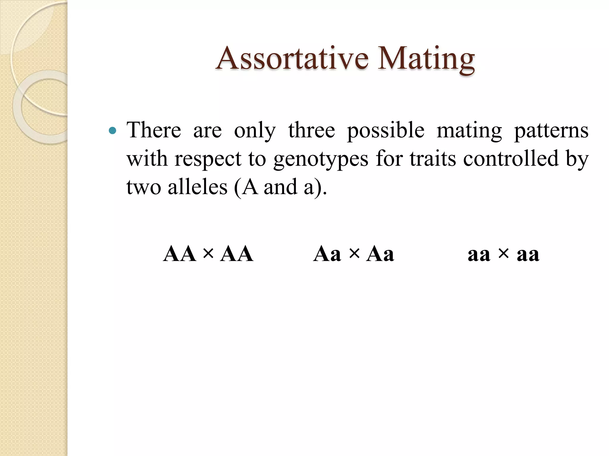
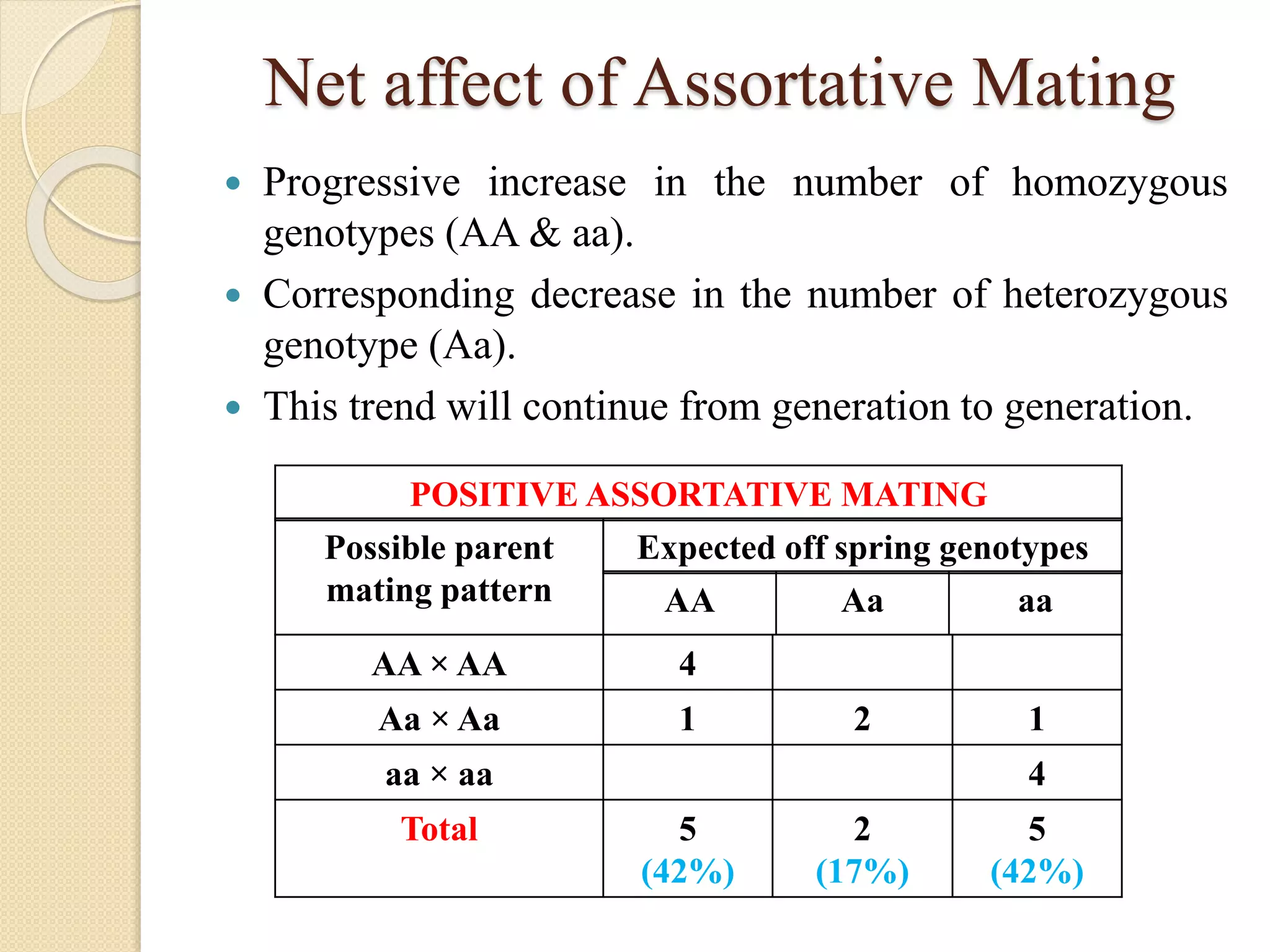
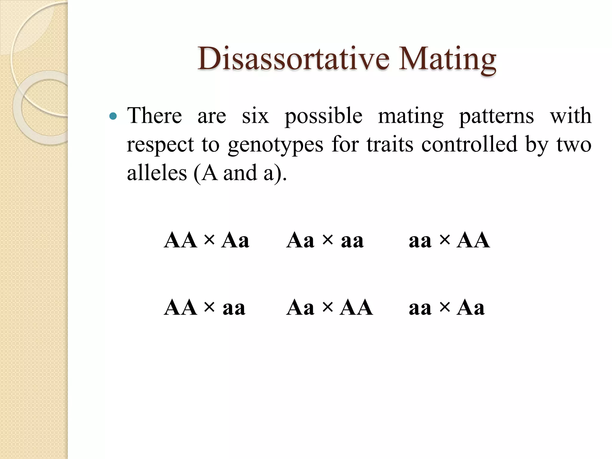
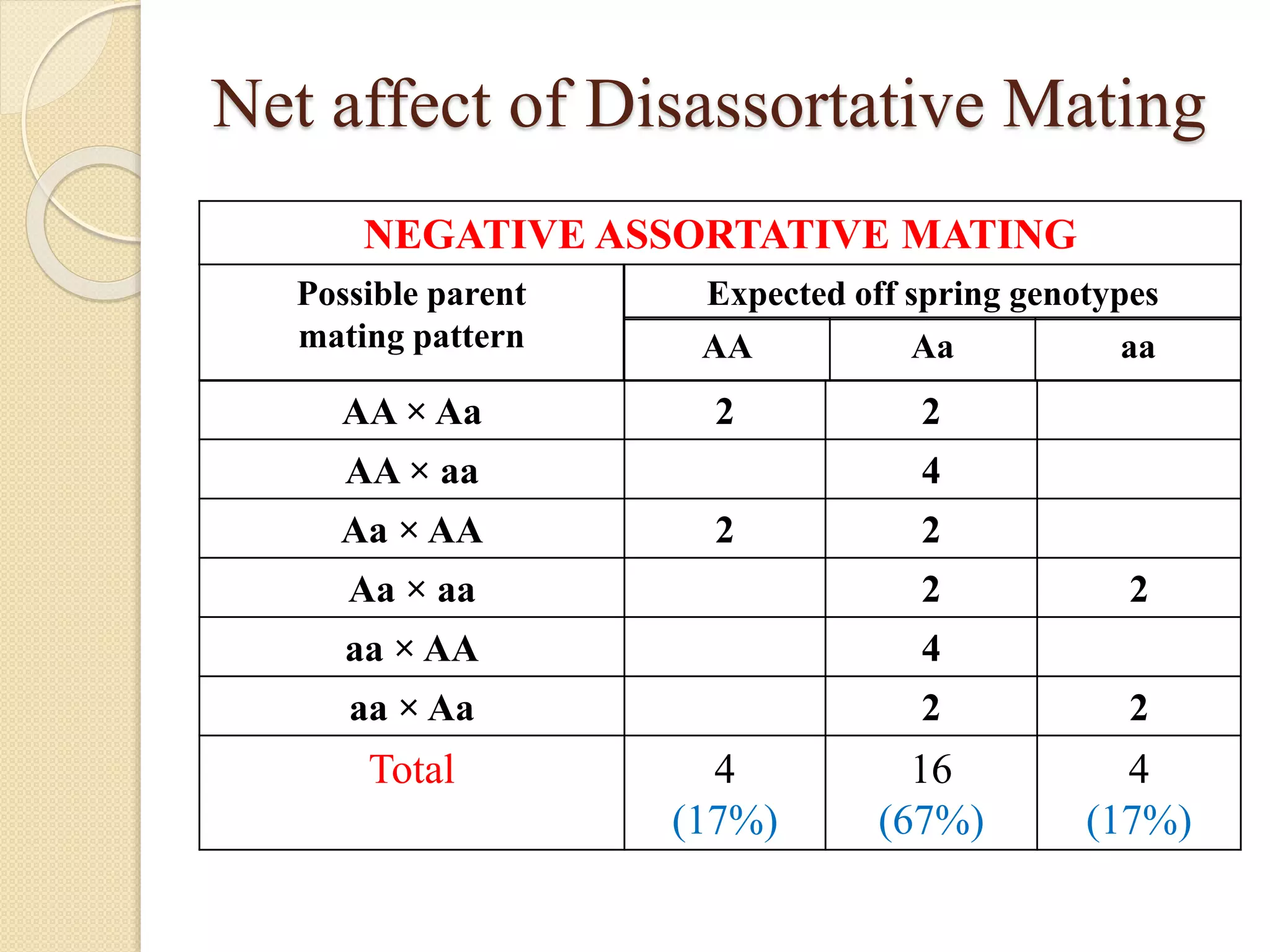
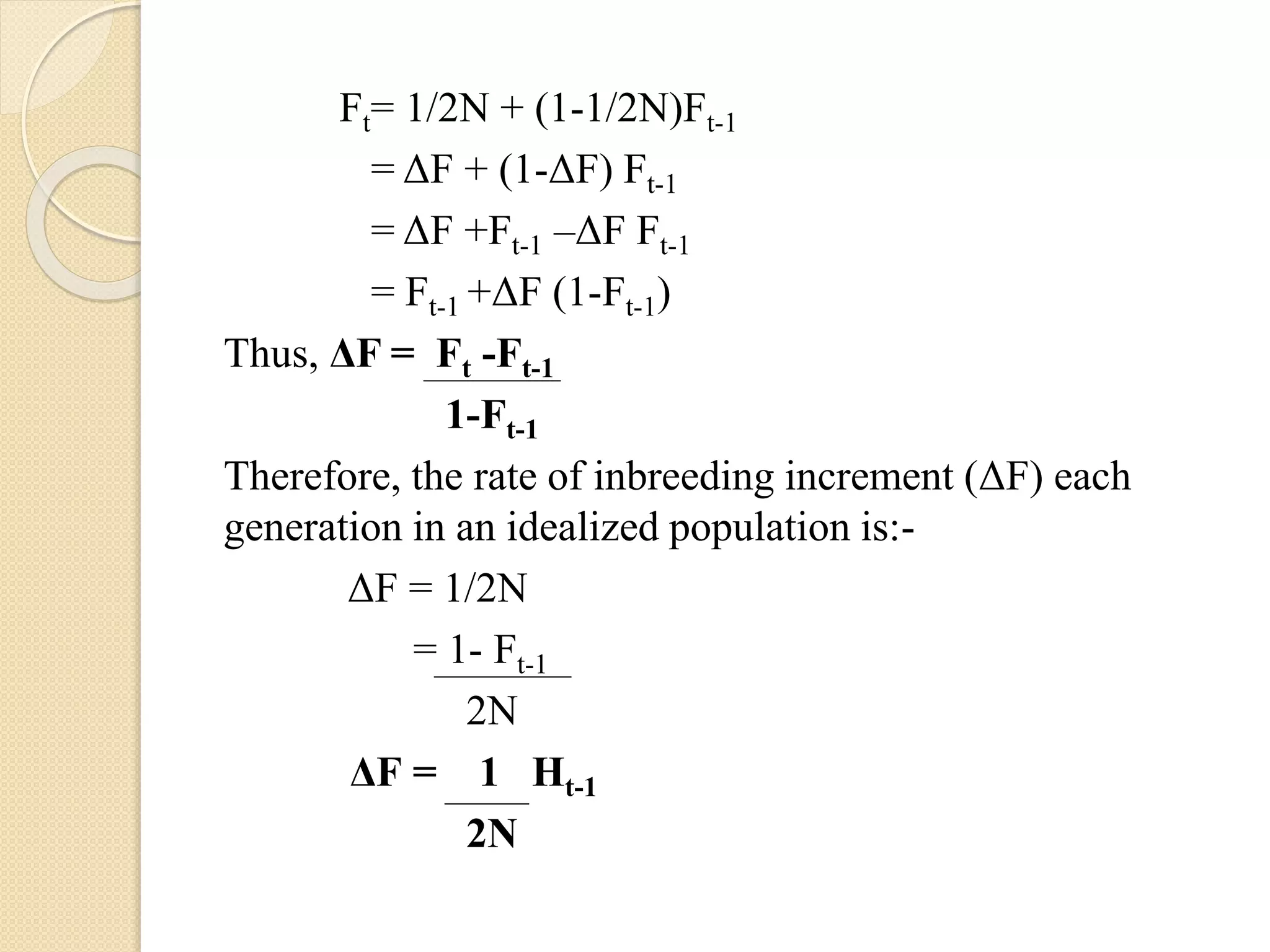
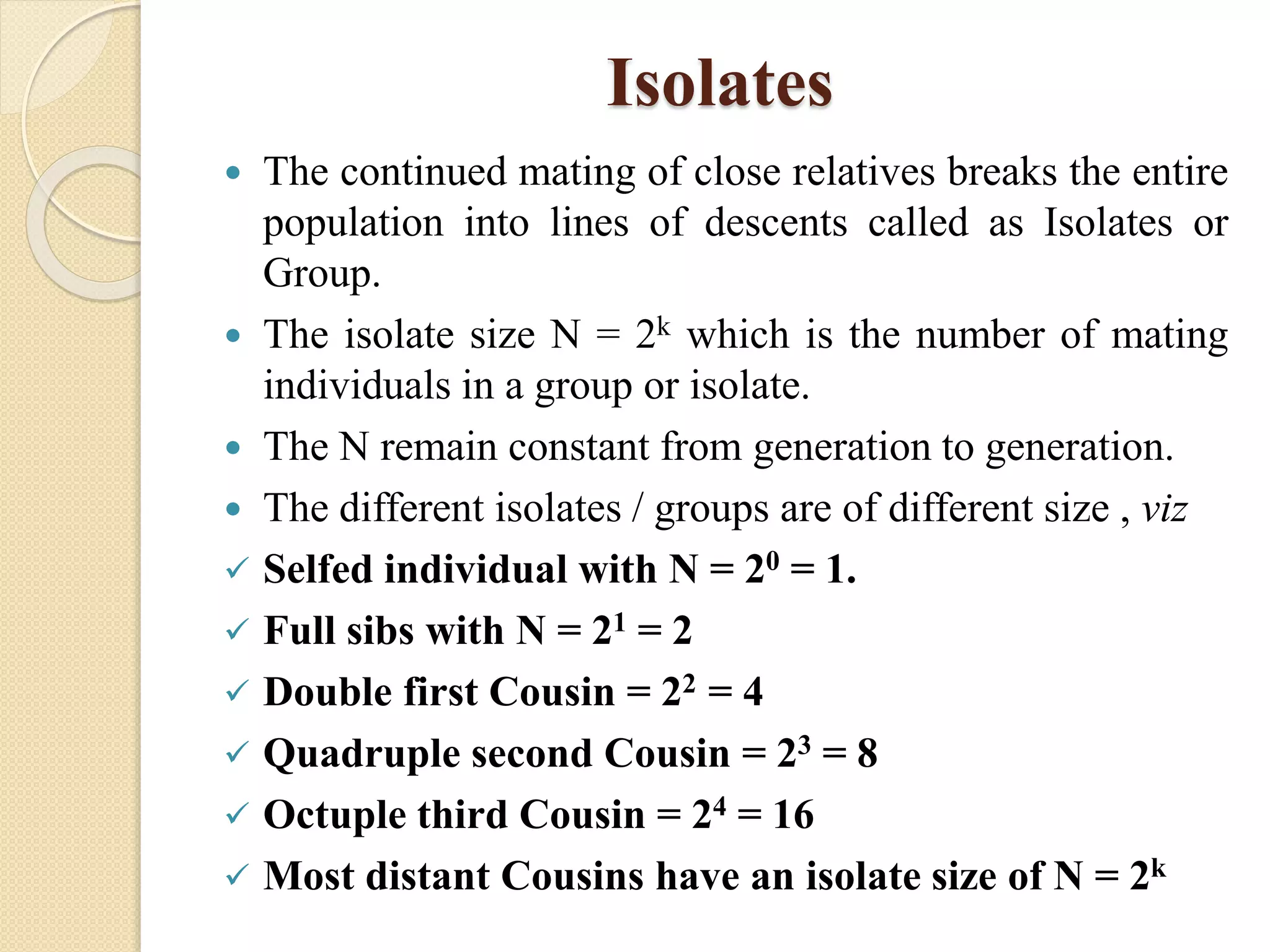
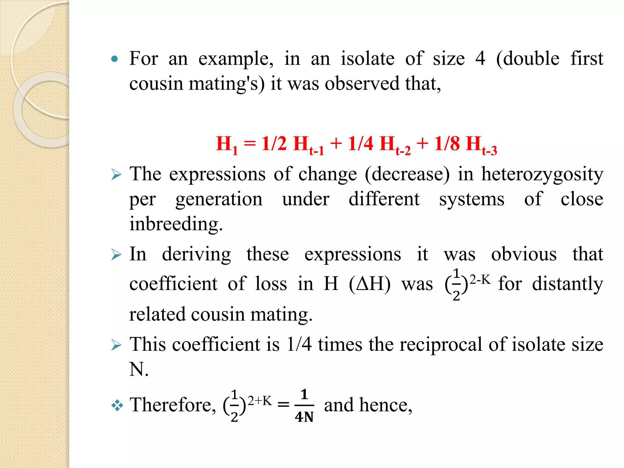
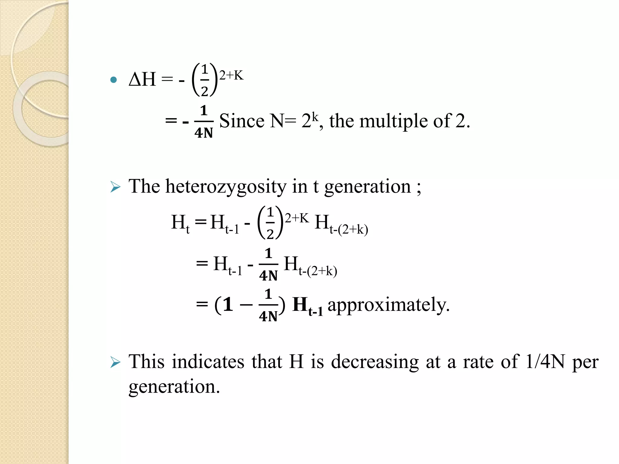
1
WELCOME
Submitted to:-
 Dr. M.P.Patel
 Professor & H.O.D,
Dept. of GPB
 SDAU, S.K. Nagar
Submitted by:-
 Vaghela Gauravrajsinh K
 M.Sc. (Agri.)
 Reg.no:-04-AGRMA-01840-2018
 SDAU, S.K. Nagar
Non Random Mating to change
Genetic Equilibrium through Inbreeding
in small population
WHAT IS RANDOM MATING?
Each male of a population has equal
chance of mating with any female of
population or vice-versa called as Random
mating or Mendelian population or
Panmixia or Panmictic population.
WHAT IS NON-RANDOM MATING?
 When the probability that two individuals in a
population will mate is not the same for all
possible pairs of individuals.
OR
 In a population male does not mating with any
female of population is called as non-random
mating.
Types of Non-Random Mating
 Disassortative- Individuals only mate with
others who are phenotypically different from
themselves for selective traits (opposites).
 Assortative- Individuals mate with others who
are like themselves phenotypically for selected
traits (similar).
Assortative Mating
 There are only three possible mating patterns
with respect to genotypes for traits controlled by
two alleles (A and a).
AA × AA Aa × Aa aa × aa
Net affect of Assortative Mating
 Progressive increase in the number of homozygous
genotypes (AA & aa).
 Corresponding decrease in the number of heterozygous
genotype (Aa).
 This trend will continue from generation to generation.
POSITIVE ASSORTATIVE MATING
Possible parent
mating pattern
Expected off spring genotypes
AA Aa aa
AA × AA 4
Aa × Aa 1 2 1
aa × aa 4
Total 5
(42%)
2
(17%)
5
(42%)
Disassortative Mating
 There are six possible mating patterns with
respect to genotypes for traits controlled by two
alleles (A and a).
AA × Aa Aa × aa aa × AA
AA × aa Aa × AA aa × Aa
Net affect of Disassortative Mating
 Progressive increase in the frequency of
heterozygotes (Aa).
 Corresponding decrease in the number of
homozygous genotypes (AA and aa).
 This trend will continue from generation to
generation.
 It has the opposite effect as Assortative mating.
Net affect of Disassortative Mating
NEGATIVE ASSORTATIVE MATING
Possible parent
mating pattern
Expected off spring genotypes
AA Aa aa
AA × Aa 2 2
AA × aa 4
Aa × AA 2 2
Aa × aa 2 2
aa × AA 4
aa × Aa 2 2
Total 4
(17%)
16
(67%)
4
(17%)
WHAT IS GENETIC EQUILIBRIUM?
 1st reported by Yule (1902), Castle (1903) and Pearson
(1904).
 W.E.Castle actually founder of genetic equilibrium
principle.
 Genetic Equilibrium means no change in genetic
structure of population (Gene & Genotype Frequency)
from one generation to the next.
 The principle of genetic equilibrium in a large random
mating population can be applied for any value of gene
frequencies.
 Therefore, this law of genetic equilibrium under random
mating is known as the Hardy-Weinberg law or
Hardy-Weinberg principle.
INBREEDING
 Mating between two individuals related by descent
(i.e having a common ancestor)
 To study the Inbreeding , there are three types of
population :-
1) Idealized population
2) Isolates
3) Real population
TYPES OF POPULATION
 Idealized population :- In which all types of mating
occur including self- fertilization. The average rate of
change in heterozygosity can be illustrated very simply
and clearly in an idealized population.
 Isolates :- Only the most distinct relatives may be
mating with maximum avoidance of inbreeding.
OR
Continue mating of close relative breaks the entire
population into lines of descents as Isolates or groups.
 Real population :- In natural or Real population , the
total no of individuals may be large but they all may not
contribute to the genetic composition of the next
generation because some of the them may not reach the
sexual maturity, other may not be able to mate while
other which mate may not leave offspring that survive to
maturity in the next generation.
 Inbreeding changes genotype frequencies not allele
frequencies.
Idealized Population
 RATE OF INBREEDING INCREMENT:-
 Consider that in an idealized population there are N
individuals, each shedding equal number of gametes
which unite at random.
 The male & female gametes produced by N individuals
can be shown as under ;
Individuals 1 2 3 Nth
Male gametes A1A2 A3A4 A5A6 A2N-1A2N
Female gametes A1A2 A3A4 A5A6 A2N-1A2N
CONT.
 Any random pairs of opposite sex gametes will have
(1/2N) chance for carrying identical genes.
F1 = 1/(2N)
 In second generation, identical homozygotes will be
produced from inbreeding in the 1st generation & from
new replication of genes.
 Probability of random pairs to be identical:- 1/(2N)
{newly replicated genes}
 Probability of remaining pairs(1-1/2N) to be identical:-
(1-1/2N)F1 {due to previous inbreeding}
F2=1/2N + (1-1/2N)F1
Ft=1/2N + (1-1/2N)Ft-1
=New Inbreeding + Old Inbreeding
CONT.
 Rate of inbreeding increment is 1/2N & symbolized by
ΔF.
Ft= 1 + Ft-1 - Ft-1
2N 2N
= Ft-1 + 1 - 1 Ft-1
2N 2N
=Ft-1 + 1 - Ft-1
2N
= Ft-1 + 1 - Ht-1 ={Old inbreeding + New
2N inbreeding(ΔF)}
CONT.
Ft= 1/2N + (1-1/2N)Ft-1
= ΔF + (1-ΔF) Ft-1
= ΔF +Ft-1 –ΔF Ft-1
= Ft-1 +ΔF (1-Ft-1)
Thus, ΔF = Ft -Ft-1
1-Ft-1
Therefore, the rate of inbreeding increment (ΔF) each
generation in an idealized population is:-
ΔF = 1/2N
= 1- Ft-1
2N
ΔF = 1 Ht-1
2N
Isolates
 The continued mating of close relatives breaks the entire
population into lines of descents called as Isolates or
Group.
 The isolate size N = 2k which is the number of mating
individuals in a group or isolate.
 The N remain constant from generation to generation.
 The different isolates / groups are of different size , viz
 Selfed individual with N = 20 = 1.
 Full sibs with N = 21 = 2
 Double first Cousin = 22 = 4
 Quadruple second Cousin = 23 = 8
 Octuple third Cousin = 24 = 16
 Most distant Cousins have an isolate size of N = 2k
 For an example, in an isolate of size 4 (double first
cousin mating's) it was observed that,
H1 = 1/2 Ht-1 + 1/4 Ht-2 + 1/8 Ht-3
 The expressions of change (decrease) in heterozygosity
per generation under different systems of close
inbreeding.
 In deriving these expressions it was obvious that
coefficient of loss in H (ΔH) was (
1
2
)2-K for distantly
related cousin mating.
 This coefficient is 1/4 times the reciprocal of isolate size
N.
 Therefore, (
1
2
)2+K =
𝟏
𝟒𝐍
and hence,
 ΔH = -
1
2
2+K
= -
𝟏
𝟒𝐍
Since N= 2k, the multiple of 2.
 The heterozygosity in t generation ;
Ht = Ht-1 -
1
2
2+K Ht-(2+k)
= Ht-1 -
𝟏
𝟒𝐍
Ht-(2+k)
= (𝟏 −
𝟏
𝟒𝐍
) Ht-1 approximately.
 This indicates that H is decreasing at a rate of 1/4N per
generation.
Real Population
 Real population do not have self fertilization, have
unequal number of breeding males and females, have
varying number of breeding individuals in different
generation, differential contribution of parents,
overlapping generations, and minimum inbreeding.
 In natural or Real population, the total no of individuals
may be large but they all may not contribute to the
genetic composition of the next generation because
some of the them may not reach the sexual maturity,
other may not be able to mate while other which mate
may not leave offspring that survive to maturity in the
next generation.
 In this male has lesser in number of contribution to
equal to that of female which are more in number.
 So number of individuals affecting genetic constitution
of next generation may be lesser than the real
population.
 Effective population size was introduced by Wright
(1931).
 In small population, there is increase in homozygosity
(inbreeding effect) and a random drift in gene
frequencies due to sampling variance.
 The concept of effective population size can be made
more clear by considering the different situations of real
population that differ from ideal population.
 The different equations for different deviated situations
will be derived situations will be derived to convert the
actual number (N) to the effective number (Ne) so as the
rate of inbreeding increment become equal in real and
ideal populations.
 The is ΔF is related to population size in an ideal
population as :- ΔF = 1/2 N
 The effective size is related is ΔF as Ne = 1/2 ΔF.
 The rate of inbreeding (ΔF) can be estimated after
knowing the effective population size as :-
ΔF = 1/2Ne
REFERENCES
1. Text book of Population Genetics (Vol. I.
Qualitative Inheritance) By S.S.Tomar.
2. Genetics By B.D.Singh
Non Random Mating to change  Genetic Equilibrium through Inbreeding  in small population

Non Random Mating to change Genetic Equilibrium through Inbreeding in small population

  • 1.
  • 2.
    Submitted to:-  Dr.M.P.Patel  Professor & H.O.D, Dept. of GPB  SDAU, S.K. Nagar Submitted by:-  Vaghela Gauravrajsinh K  M.Sc. (Agri.)  Reg.no:-04-AGRMA-01840-2018  SDAU, S.K. Nagar Non Random Mating to change Genetic Equilibrium through Inbreeding in small population
  • 3.
    WHAT IS RANDOMMATING? Each male of a population has equal chance of mating with any female of population or vice-versa called as Random mating or Mendelian population or Panmixia or Panmictic population.
  • 4.
    WHAT IS NON-RANDOMMATING?  When the probability that two individuals in a population will mate is not the same for all possible pairs of individuals. OR  In a population male does not mating with any female of population is called as non-random mating.
  • 5.
    Types of Non-RandomMating  Disassortative- Individuals only mate with others who are phenotypically different from themselves for selective traits (opposites).  Assortative- Individuals mate with others who are like themselves phenotypically for selected traits (similar).
  • 6.
    Assortative Mating  Thereare only three possible mating patterns with respect to genotypes for traits controlled by two alleles (A and a). AA × AA Aa × Aa aa × aa
  • 7.
    Net affect ofAssortative Mating  Progressive increase in the number of homozygous genotypes (AA & aa).  Corresponding decrease in the number of heterozygous genotype (Aa).  This trend will continue from generation to generation. POSITIVE ASSORTATIVE MATING Possible parent mating pattern Expected off spring genotypes AA Aa aa AA × AA 4 Aa × Aa 1 2 1 aa × aa 4 Total 5 (42%) 2 (17%) 5 (42%)
  • 8.
    Disassortative Mating  Thereare six possible mating patterns with respect to genotypes for traits controlled by two alleles (A and a). AA × Aa Aa × aa aa × AA AA × aa Aa × AA aa × Aa
  • 9.
    Net affect ofDisassortative Mating  Progressive increase in the frequency of heterozygotes (Aa).  Corresponding decrease in the number of homozygous genotypes (AA and aa).  This trend will continue from generation to generation.  It has the opposite effect as Assortative mating.
  • 10.
    Net affect ofDisassortative Mating NEGATIVE ASSORTATIVE MATING Possible parent mating pattern Expected off spring genotypes AA Aa aa AA × Aa 2 2 AA × aa 4 Aa × AA 2 2 Aa × aa 2 2 aa × AA 4 aa × Aa 2 2 Total 4 (17%) 16 (67%) 4 (17%)
  • 11.
    WHAT IS GENETICEQUILIBRIUM?  1st reported by Yule (1902), Castle (1903) and Pearson (1904).  W.E.Castle actually founder of genetic equilibrium principle.  Genetic Equilibrium means no change in genetic structure of population (Gene & Genotype Frequency) from one generation to the next.  The principle of genetic equilibrium in a large random mating population can be applied for any value of gene frequencies.  Therefore, this law of genetic equilibrium under random mating is known as the Hardy-Weinberg law or Hardy-Weinberg principle.
  • 12.
    INBREEDING  Mating betweentwo individuals related by descent (i.e having a common ancestor)  To study the Inbreeding , there are three types of population :- 1) Idealized population 2) Isolates 3) Real population
  • 13.
    TYPES OF POPULATION Idealized population :- In which all types of mating occur including self- fertilization. The average rate of change in heterozygosity can be illustrated very simply and clearly in an idealized population.  Isolates :- Only the most distinct relatives may be mating with maximum avoidance of inbreeding. OR Continue mating of close relative breaks the entire population into lines of descents as Isolates or groups.
  • 14.
     Real population:- In natural or Real population , the total no of individuals may be large but they all may not contribute to the genetic composition of the next generation because some of the them may not reach the sexual maturity, other may not be able to mate while other which mate may not leave offspring that survive to maturity in the next generation.  Inbreeding changes genotype frequencies not allele frequencies.
  • 15.
    Idealized Population  RATEOF INBREEDING INCREMENT:-  Consider that in an idealized population there are N individuals, each shedding equal number of gametes which unite at random.  The male & female gametes produced by N individuals can be shown as under ; Individuals 1 2 3 Nth Male gametes A1A2 A3A4 A5A6 A2N-1A2N Female gametes A1A2 A3A4 A5A6 A2N-1A2N CONT.
  • 16.
     Any randompairs of opposite sex gametes will have (1/2N) chance for carrying identical genes. F1 = 1/(2N)  In second generation, identical homozygotes will be produced from inbreeding in the 1st generation & from new replication of genes.  Probability of random pairs to be identical:- 1/(2N) {newly replicated genes}  Probability of remaining pairs(1-1/2N) to be identical:- (1-1/2N)F1 {due to previous inbreeding} F2=1/2N + (1-1/2N)F1 Ft=1/2N + (1-1/2N)Ft-1 =New Inbreeding + Old Inbreeding CONT.
  • 17.
     Rate ofinbreeding increment is 1/2N & symbolized by ΔF. Ft= 1 + Ft-1 - Ft-1 2N 2N = Ft-1 + 1 - 1 Ft-1 2N 2N =Ft-1 + 1 - Ft-1 2N = Ft-1 + 1 - Ht-1 ={Old inbreeding + New 2N inbreeding(ΔF)} CONT.
  • 18.
    Ft= 1/2N +(1-1/2N)Ft-1 = ΔF + (1-ΔF) Ft-1 = ΔF +Ft-1 –ΔF Ft-1 = Ft-1 +ΔF (1-Ft-1) Thus, ΔF = Ft -Ft-1 1-Ft-1 Therefore, the rate of inbreeding increment (ΔF) each generation in an idealized population is:- ΔF = 1/2N = 1- Ft-1 2N ΔF = 1 Ht-1 2N
  • 19.
    Isolates  The continuedmating of close relatives breaks the entire population into lines of descents called as Isolates or Group.  The isolate size N = 2k which is the number of mating individuals in a group or isolate.  The N remain constant from generation to generation.  The different isolates / groups are of different size , viz  Selfed individual with N = 20 = 1.  Full sibs with N = 21 = 2  Double first Cousin = 22 = 4  Quadruple second Cousin = 23 = 8  Octuple third Cousin = 24 = 16  Most distant Cousins have an isolate size of N = 2k
  • 20.
     For anexample, in an isolate of size 4 (double first cousin mating's) it was observed that, H1 = 1/2 Ht-1 + 1/4 Ht-2 + 1/8 Ht-3  The expressions of change (decrease) in heterozygosity per generation under different systems of close inbreeding.  In deriving these expressions it was obvious that coefficient of loss in H (ΔH) was ( 1 2 )2-K for distantly related cousin mating.  This coefficient is 1/4 times the reciprocal of isolate size N.  Therefore, ( 1 2 )2+K = 𝟏 𝟒𝐍 and hence,
  • 21.
     ΔH =- 1 2 2+K = - 𝟏 𝟒𝐍 Since N= 2k, the multiple of 2.  The heterozygosity in t generation ; Ht = Ht-1 - 1 2 2+K Ht-(2+k) = Ht-1 - 𝟏 𝟒𝐍 Ht-(2+k) = (𝟏 − 𝟏 𝟒𝐍 ) Ht-1 approximately.  This indicates that H is decreasing at a rate of 1/4N per generation.
  • 22.
    Real Population  Realpopulation do not have self fertilization, have unequal number of breeding males and females, have varying number of breeding individuals in different generation, differential contribution of parents, overlapping generations, and minimum inbreeding.  In natural or Real population, the total no of individuals may be large but they all may not contribute to the genetic composition of the next generation because some of the them may not reach the sexual maturity, other may not be able to mate while other which mate may not leave offspring that survive to maturity in the next generation.
  • 23.
     In thismale has lesser in number of contribution to equal to that of female which are more in number.  So number of individuals affecting genetic constitution of next generation may be lesser than the real population.  Effective population size was introduced by Wright (1931).  In small population, there is increase in homozygosity (inbreeding effect) and a random drift in gene frequencies due to sampling variance.
  • 24.
     The conceptof effective population size can be made more clear by considering the different situations of real population that differ from ideal population.  The different equations for different deviated situations will be derived situations will be derived to convert the actual number (N) to the effective number (Ne) so as the rate of inbreeding increment become equal in real and ideal populations.  The is ΔF is related to population size in an ideal population as :- ΔF = 1/2 N  The effective size is related is ΔF as Ne = 1/2 ΔF.  The rate of inbreeding (ΔF) can be estimated after knowing the effective population size as :- ΔF = 1/2Ne
  • 25.
    REFERENCES 1. Text bookof Population Genetics (Vol. I. Qualitative Inheritance) By S.S.Tomar. 2. Genetics By B.D.Singh