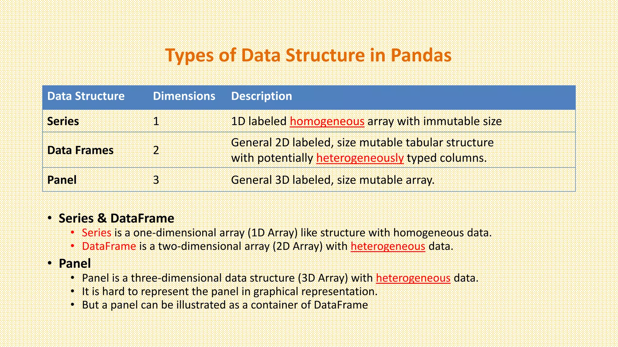
![Creating a DataFrame from scratch
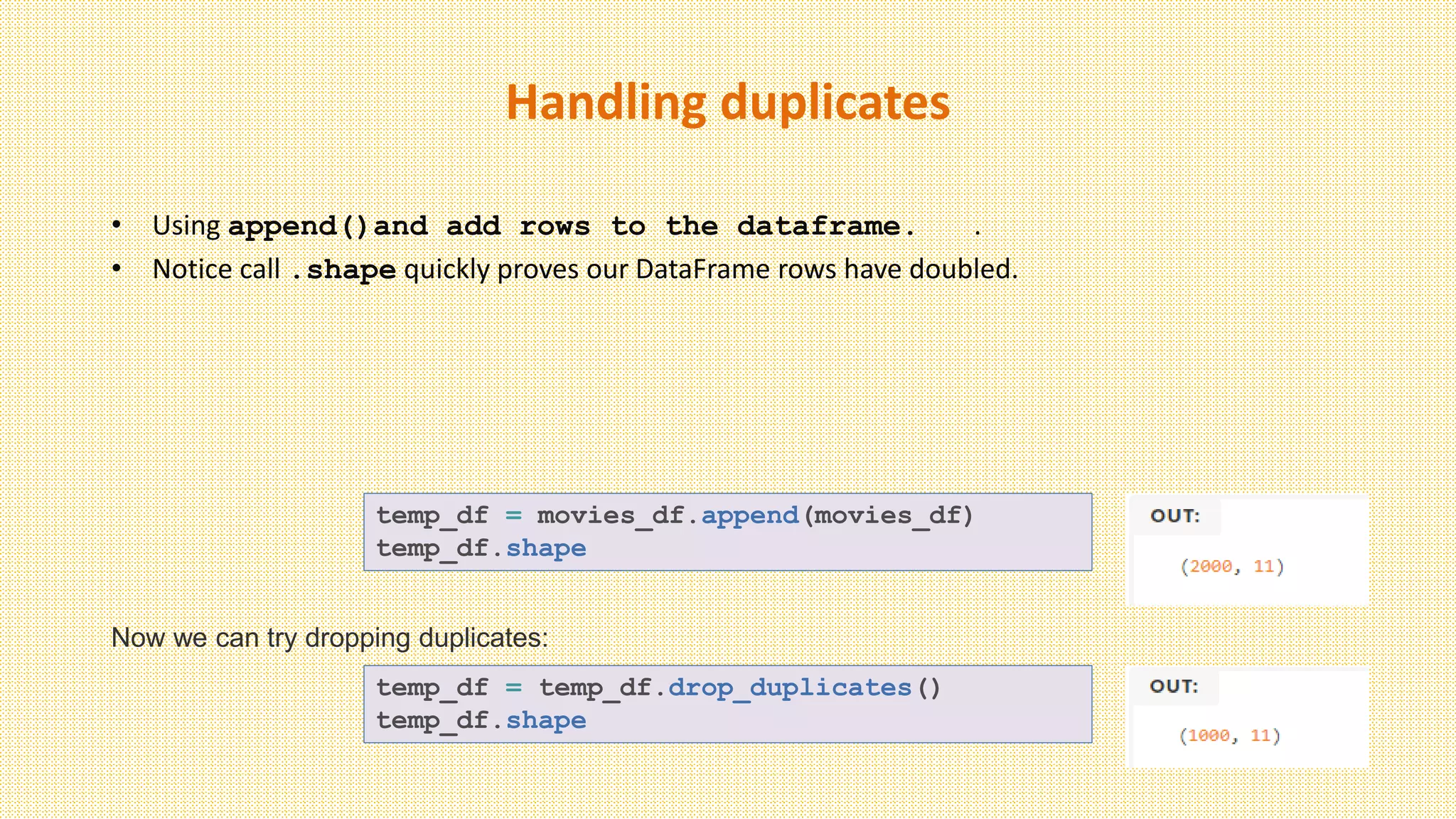
• There are many ways to create a DataFrame from scratch, but a great option is
to just use a simple dict. But first you must import pandas.
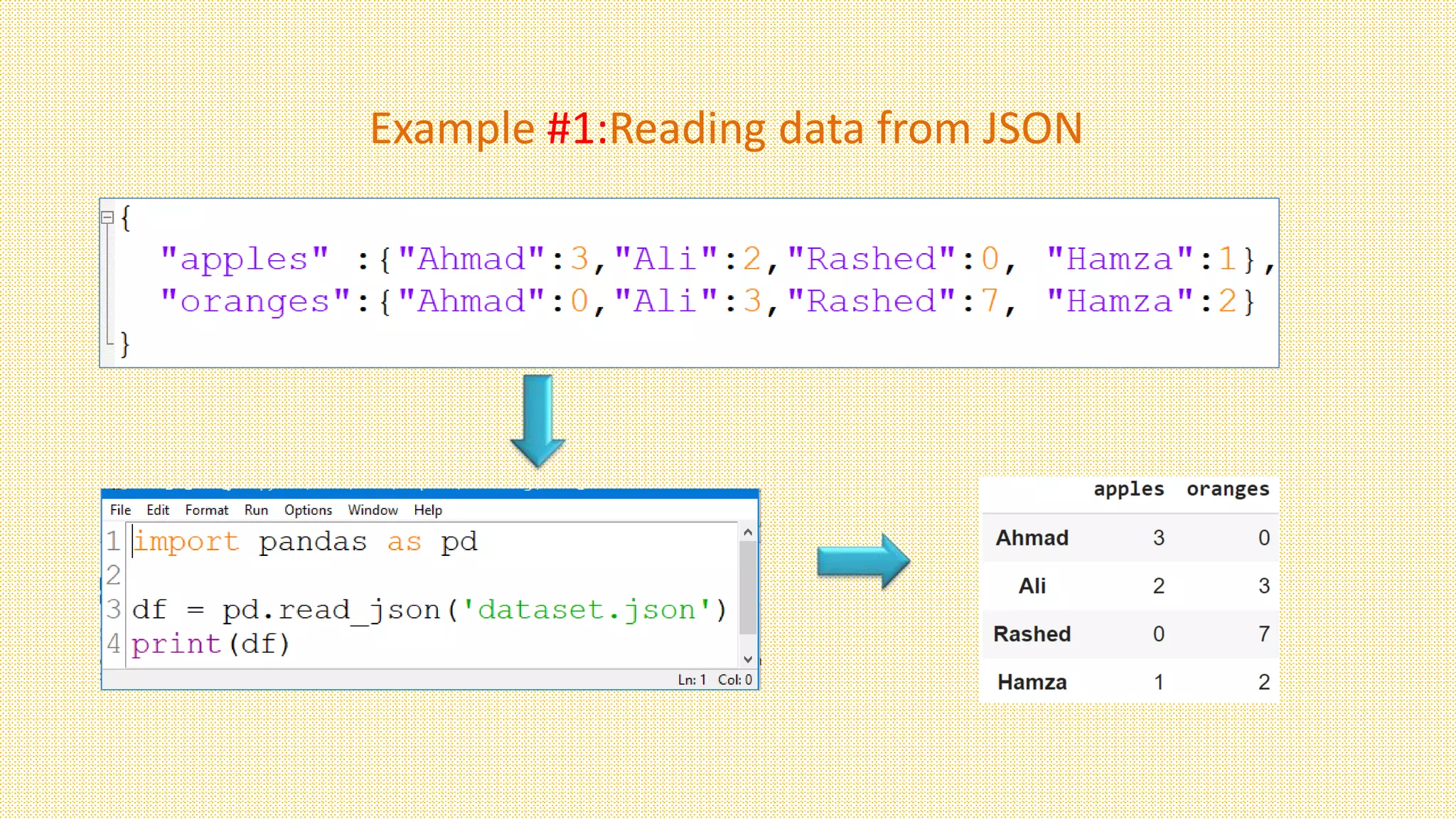
• Let's say we have a fruit stand that sells apples and oranges. We want to have a column for
each fruit and a row for each customer purchase. To organize this as a dictionary for pandas
we could do something like:
• And then pass it to the pandas DataFrame constructor:
df = pd.DataFrame(data)
import pandas as pd
data = { 'apples':[3, 2, 0, 1] , 'oranges':[0, 3, 7, 2] }](https://image.slidesharecdn.com/l3pandasdataframereadingdatakirtifinal-230902174839-cd369e29/75/Pandas-Dataframe-reading-data-Kirti-final-pptx-8-2048.jpg)
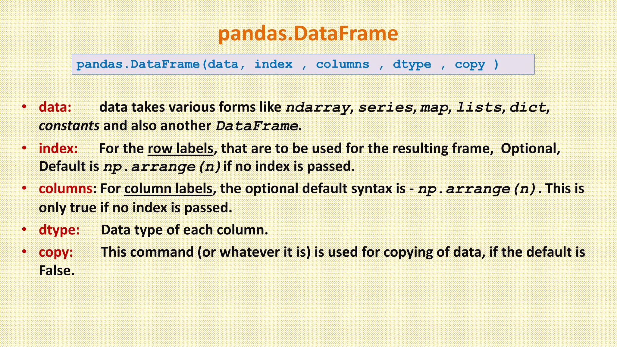
![Setting Index
• Each (key, value) item in data corresponds to a column in the resulting DataFrame.
• The Index of this DataFrame was given to us on creation as the numbers 0-3, but we could
also create our own when we initialize the DataFrame.
• E.g. if you want to have customer names as the index:
• So now we could locate a customer's
order by using their names:
df = pd.DataFrame(data, index=['Ahmad', 'Ali', 'Rashed', 'Hamza'])
df.loc['Ali']](https://image.slidesharecdn.com/l3pandasdataframereadingdatakirtifinal-230902174839-cd369e29/75/Pandas-Dataframe-reading-data-Kirti-final-pptx-9-2048.jpg)
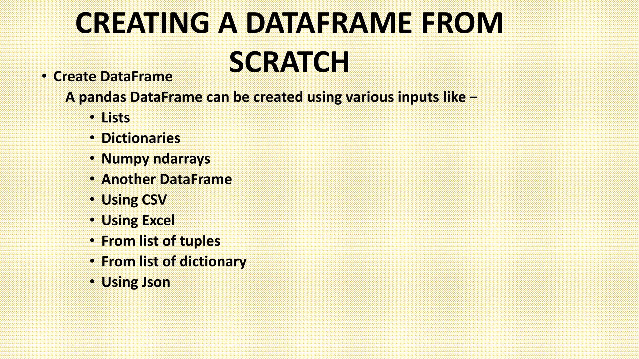
![pandas’ orient keyword
data = {'col_1':[3, 2, 1, 0], 'col_2':['a','b','c','d']}
pd.DataFrame.from_dict(data)
data = {'row_1':[3, 2, 1, 0], 'row_2':['a','b','c','d']}
pd.DataFrame.from_dict(data,
orient='index')
data = {'row_1':[3, 2, 1, 0], 'row_2':['a','b','c','d']}
pd.DataFrame.from_dict(data,
orient = 'index',
columns = ['A','B','C','D'])](https://image.slidesharecdn.com/l3pandasdataframereadingdatakirtifinal-230902174839-cd369e29/75/Pandas-Dataframe-reading-data-Kirti-final-pptx-11-2048.jpg)
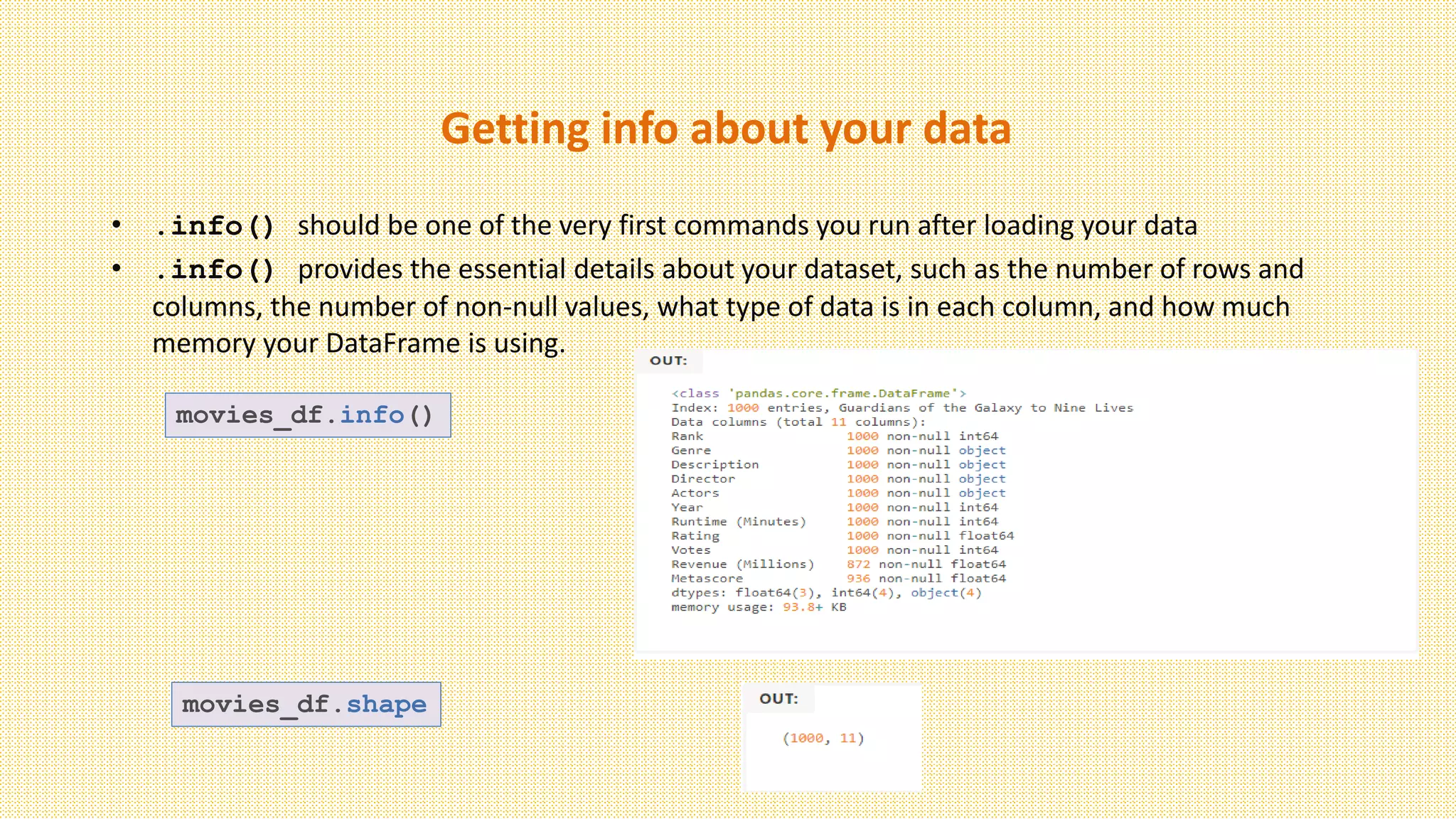
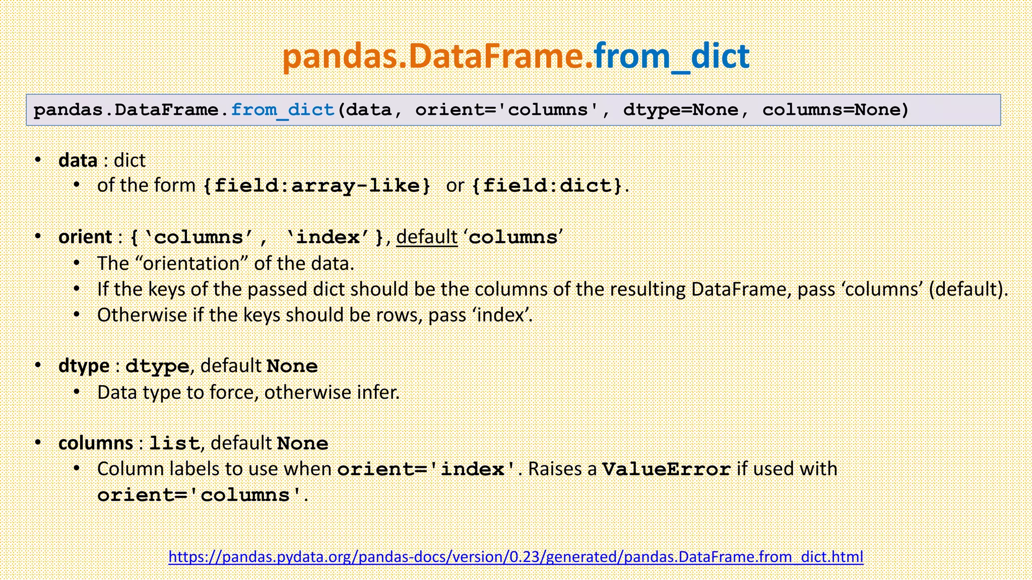
![Understanding your variables
• Using .describe() on an entire DataFrame we can get a summary of the numeric data
• .describe() can also be used on a categorical variable to get the count of rows, unique
count of categories, top category, and freq of top category:
• This tells us that the genre column has 207 unique values, the top value is Action/Adventure/Sci-
Fi, which shows up 50 times (freq).
movies_df.describe()
movies_df['genre'].describe()](https://image.slidesharecdn.com/l3pandasdataframereadingdatakirtifinal-230902174839-cd369e29/75/Pandas-Dataframe-reading-data-Kirti-final-pptx-22-2048.jpg)
![DataFrame having Missing values& assigning new index to
DataFrame
import pandas as pd
data = [{'a': 1, 'b': 2},{'a': 5, 'b': 10, 'c': 20}]
df = pd.DataFrame(data)
print(df)
import pandas as pd
data = [{'a': 1, 'b': 2},{'a': 5, 'b': 10, 'c': 20}]
df = pd.DataFrame(data, index=['first', 'second'])
print(df)
a b c
0 1 2 NaN
1 5 10 20.0
a b c
first 1 2 NaN
second 5 10 20.0](https://image.slidesharecdn.com/l3pandasdataframereadingdatakirtifinal-230902174839-cd369e29/75/Pandas-Dataframe-reading-data-Kirti-final-pptx-23-2048.jpg)
![Using new column name
import pandas as pd
data = [{'a': 1, 'b': 2},{'a': 5, 'b': 10, 'c': 20}]
#With two column indices, values same as dictionary keys
df1 = pd.DataFrame(data,index=['first','second'],columns=['a','b'])
#With two column indices with one index with other name
df2 = pd.DataFrame(data,index=['first','second'],columns=['a','b1'])
print(df1)
print('...........')
print(df2)
E.g. This shows how to create a DataFrame with a list of dictionaries, row indices, and column indices.
a b
first 1 2
second 5 10
...........
a b1
first 1 NaN
second 5 NaN](https://image.slidesharecdn.com/l3pandasdataframereadingdatakirtifinal-230902174839-cd369e29/75/Pandas-Dataframe-reading-data-Kirti-final-pptx-24-2048.jpg)
![Adding Column: As series & as sum of columns
import pandas as pd
d = {'one':pd.Series([1,2,3], index=['a','b','c']),
'two':pd.Series([1,2,3,4], index=['a','b','c','d'])
}
df = pd.DataFrame(d)
# Adding a new column to an existing DataFrame object
# with column label by passing new series
print("Adding a new column by passing as Series:")
df['three'] = pd.Series([10,20,30],index=['a','b','c'])
print(df)
print("Adding a column using an existing columns in
DataFrame:")
df['four'] = df['one']+df['three']
print(df)
Adding a column using Series:
one two three
a 1.0 1 10.0
b 2.0 2 20.0
c 3.0 3 30.0
d NaN 4 NaN
Adding a column using columns:
one two three four
a 1.0 1 10.0 11.0
b 2.0 2 20.0 22.0
c 3.0 3 30.0 33.0
d NaN 4 NaN NaN](https://image.slidesharecdn.com/l3pandasdataframereadingdatakirtifinal-230902174839-cd369e29/75/Pandas-Dataframe-reading-data-Kirti-final-pptx-25-2048.jpg)
![Column Deletion using Del and pop()
# Using the previous DataFrame, we will delete a column
# using del function
import pandas as pd
d = {'one' : pd.Series([1, 2, 3], index=['a', 'b', 'c']),
'two' : pd.Series([1, 2, 3, 4], index=['a', 'b', 'c', 'd']),
'three' : pd.Series([10,20,30], index=['a','b','c'])
}
df = pd.DataFrame(d)
print ("Our dataframe is:")
print(df)
# using del function
print("Deleting the first column using DEL function:")
del df['one']
print(df)
# using pop function
print("Deleting another column using POP function:")
df.pop('two')
print(df)
Our dataframe is:
one two three
a 1.0 1 10.0
b 2.0 2 20.0
c 3.0 3 30.0
d NaN 4 NaN
Deleting the first column:
two three
a 1 10.0
b 2 20.0
c 3 30.0
d 4 NaN
Deleting another column:
a 10.0
b 20.0
c 30.0
d NaN](https://image.slidesharecdn.com/l3pandasdataframereadingdatakirtifinal-230902174839-cd369e29/75/Pandas-Dataframe-reading-data-Kirti-final-pptx-26-2048.jpg)
![Slicing in DataFrames
import pandas as pd
d = {'one' : pd.Series([1, 2, 3], index=['a', 'b', 'c']),
'two' : pd.Series([1, 2, 3, 4], index=['a', 'b', 'c','d'])
}
df = pd.DataFrame(d)
print(df[2:4])
one two
c 3.0 3
d NaN 4](https://image.slidesharecdn.com/l3pandasdataframereadingdatakirtifinal-230902174839-cd369e29/75/Pandas-Dataframe-reading-data-Kirti-final-pptx-27-2048.jpg)
![Addition of rows to existing dataframe
import pandas as pd
d = {'one' : pd.Series([1, 2, 3], index=['a', 'b', 'c']),
'two' : pd.Series([1, 2, 3, 4], index=['a', 'b', 'c','d'])
}
df = pd.DataFrame(d)
print(df)
df2 = pd.DataFrame([[5,6], [7,8]], columns = ['a', 'b'])
df = df.append(df2 )
print(df)
one two
a 1.0 1
b 2.0 2
c 3.0 3
d NaN 4
one two a b
a 1.0 1.0 NaN NaN
b 2.0 2.0 NaN NaN
c 3.0 3.0 NaN NaN
d NaN 4.0 NaN NaN
0 NaN NaN 5.0 6.0
1 NaN NaN 7.0 8.0](https://image.slidesharecdn.com/l3pandasdataframereadingdatakirtifinal-230902174839-cd369e29/75/Pandas-Dataframe-reading-data-Kirti-final-pptx-28-2048.jpg)
![Deletion of rows
import pandas as pd
d = {'one':pd.Series([1, 2, 3], index=['a','b','c']),
'two':pd.Series([1, 2, 3, 4], index=['a','b','c','d'])
}
df = pd.DataFrame(d)
print(df)
df2 = pd.DataFrame([[5,6], [7,8]], columns = ['a', 'b'])
df = df.append(df2 )
print(df)
df = df.drop(0)
print(df)
one two
a 1.0 1
b 2.0 2
c 3.0 3
d NaN 4
one two a b
a 1.0 1.0 NaN NaN
b 2.0 2.0 NaN NaN
c 3.0 3.0 NaN NaN
d NaN 4.0 NaN NaN
0 NaN NaN 5.0 6.0
1 NaN NaN 7.0 8.0
one two a b
a 1.0 1.0 NaN NaN
b 2.0 2.0 NaN NaN
c 3.0 3.0 NaN NaN
d NaN 4.0 NaN NaN
1 NaN NaN 7.0 8.0](https://image.slidesharecdn.com/l3pandasdataframereadingdatakirtifinal-230902174839-cd369e29/75/Pandas-Dataframe-reading-data-Kirti-final-pptx-29-2048.jpg)
![Reindexing
import pandas as pd
# Creating the first dataframe
df1 = pd.DataFrame({"A":[1, 5, 3, 4, 2],
"B":[3, 2, 4, 3, 4],
"C":[2, 2, 7, 3, 4],
"D":[4, 3, 6, 12, 7]},
index =["A1", "A2", "A3", "A4", "A5"])
# Creating the second dataframe
df2 = pd.DataFrame({"A":[10, 11, 7, 8, 5],
"B":[21, 5, 32, 4, 6],
"C":[11, 21, 23, 7, 9],
"D":[1, 5, 3, 8, 6]},
index =["A1", "A3", "A4", "A7", "A8"])
# Print the first dataframe
print(df1)
print(df2)
# find matching indexes
df1.reindex_like(df2)
• Pandas
dataframe.reindex_like()
function return an object with
matching indices to myself.
• Any non-matching indexes are filled
with NaN values.](https://image.slidesharecdn.com/l3pandasdataframereadingdatakirtifinal-230902174839-cd369e29/75/Pandas-Dataframe-reading-data-Kirti-final-pptx-30-2048.jpg)
![Concatenating Objects (Data Frames)
import pandas as pd
df1 = pd.DataFrame({'Name':['A','B'], 'SSN':[10,20], 'marks':[90, 95] })
df2 = pd.DataFrame({'Name':['B','C'], 'SSN':[25,30], 'marks':[80, 97] })
df3 = pd.concat([df1, df2])
df3](https://image.slidesharecdn.com/l3pandasdataframereadingdatakirtifinal-230902174839-cd369e29/75/Pandas-Dataframe-reading-data-Kirti-final-pptx-31-2048.jpg)


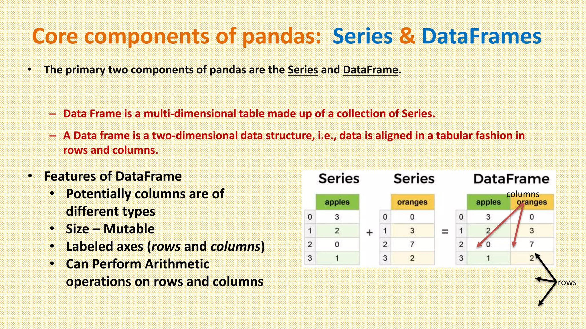
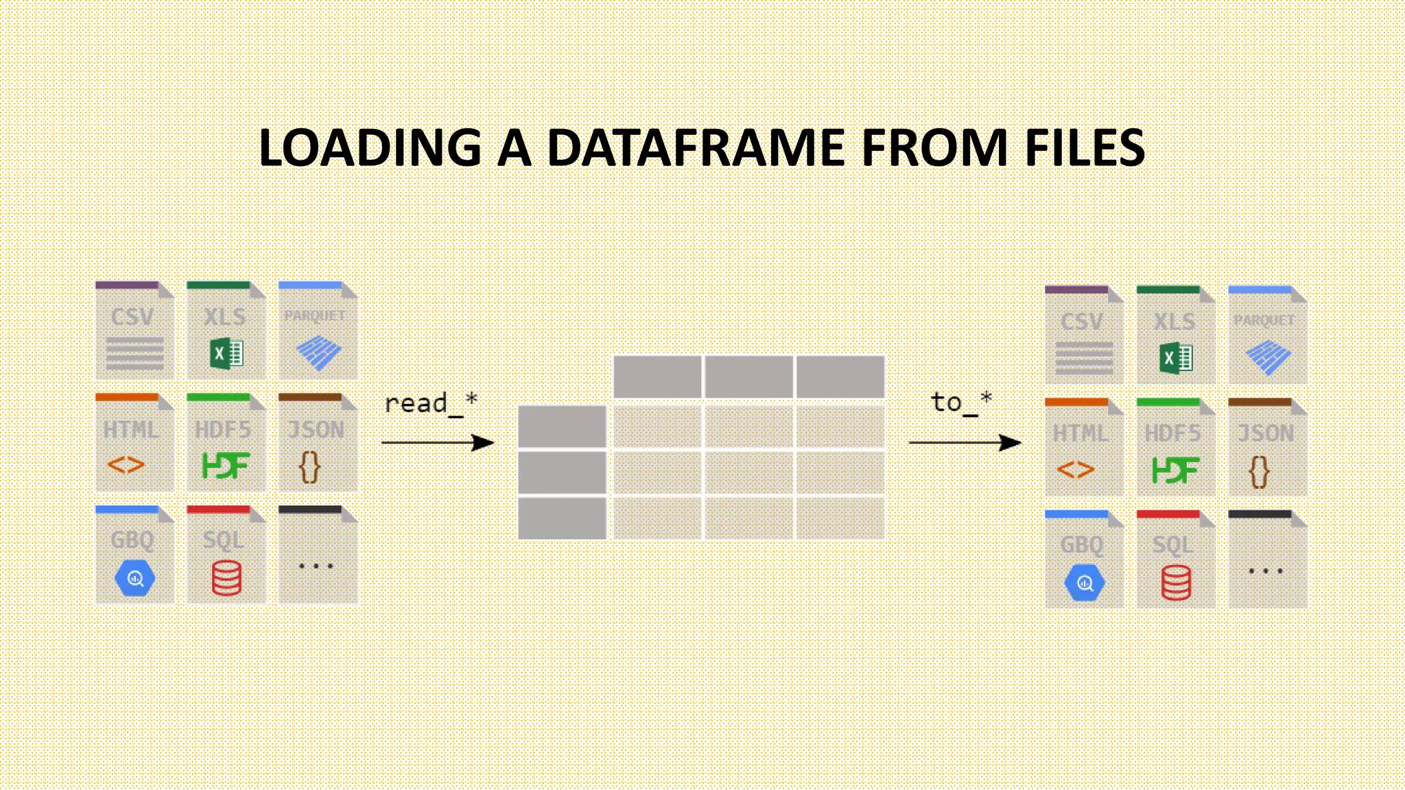
Pandas is a Python library used for data manipulation and analysis. It provides data structures like Series and DataFrames that make working with structured data easy. A DataFrame is a two-dimensional data structure that can store data of different types in columns. DataFrames can be created from dictionaries, lists, CSV files, JSON files and other sources. They allow indexing, selecting, adding and deleting of rows and columns. Pandas provides useful methods for data cleaning, manipulation and analysis tasks on DataFrames.


![Introduction to Pandas and Time Series Analysis [PyCon DE]](https://cdn.slidesharecdn.com/ss_thumbnails/introductiontopandasandtimeseriesanalysispyconde-170617163724-thumbnail.jpg?width=640&height=640&fit=bounds)