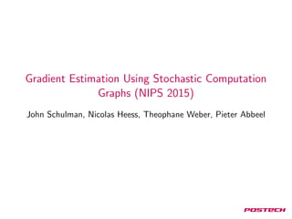
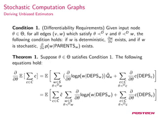
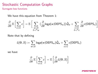
The document discusses stochastic gradient estimation using stochastic computation graphs, which are essential in various applications such as computational finance, reinforcement learning, and neural networks. It introduces different gradient estimation approaches, including score function and pathwise derivative estimators, highlighting their advantages and disadvantages. Furthermore, it emphasizes the versatility of stochastic computation graphs in expressing multiple algorithms and their capacity to unify diverse methods in machine learning.

1. Gradient Estimation Using Stochastic
Computation Graphs
Yoonho Lee
Department of Computer Science and Engineering
Pohang University of Science and Technology
May 9, 2017

2. Outline
Stochastic Gradient Estimation
Stochastic Computation Graphs
Stochastic Computation Graphs in RL
Other Examples of Stochastic Computation Graphs

3. Outline
Stochastic Gradient Estimation
Stochastic Computation Graphs
Stochastic Computation Graphs in RL
Other Examples of Stochastic Computation Graphs

4. Stochastic Gradient Estimation
R(θ) = Ew∼Pθ(dw)[f (θ, w)]
Approximate θR(θ) can be used for:
Computational Finance
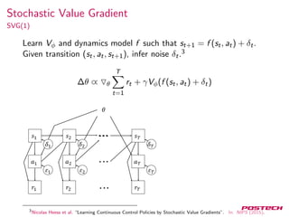
Reinforcement Learning
Variational Inference
Explaining the brain with neural networks

5. Stochastic Gradient Estimation
R(θ) = Ew∼Pθ(dw)[f (θ, w)] =
Ω
f (θ, w)Pθ(dw)

6. Stochastic Gradient Estimation
R(θ) = Ew∼Pθ(dw)[f (θ, w)] =
Ω
f (θ, w)Pθ(dw)
=
Ω
f (θ, w)
Pθ(dw)
G(dw)
G(dw)

7. Stochastic Gradient Estimation
R(θ) = Ew∼Pθ(dw)[f (θ, w)] =
Ω
f (θ, w)Pθ(dw)
=
Ω
f (θ, w)
Pθ(dw)
G(dw)
G(dw)
θR(θ) = θ
Ω
f (θ, w)
Pθ(dw)
G(dw)
G(dw)
=
Ω
θ(f (θ, w)
Pθ(dw)
G(dw)
)G(dw)
= Ew∼G(dw)[ θf (θ, w)
Pθ(dw)
G(dw)
+ f (θ, w)
θPθ(dw)
G(dw)
]

8. Stochastic Gradient Estimation
So far we have
θR(θ) = Ew∼G(dw)[ θf (θ, w)
Pθ(dw)
G(dw)
+ f (θ, w)
θPθ(dw)
G(dw)
]

9. Stochastic Gradient Estimation
So far we have
θR(θ) = Ew∼G(dw)[ θf (θ, w)
Pθ(dw)
G(dw)
+ f (θ, w)
θPθ(dw)
G(dw)
]
Letting G = Pθ0 and evaluating at θ = θ0, we get
θR(θ)
θ=θ0
= Ew∼Pθ0
(dw)[ θf (θ, w)
Pθ(dw)
Pθ0 (dw)
+ f (θ, w)
θPθ(dw)
Pθ0 (dw)
]
θ=θ0
= Ew∼Pθ0
(dw)[ θf (θ, w) + f (θ, w) θlnPθ(dw)]
θ=θ0

10. Stochastic Gradient Estimation
So far we have
R(θ) = Ew∼Pθ(dw)[f (θ, w)]
θR(θ)
θ=θ0
= Ew∼Pθ0
(dw)[ θf (θ, w) + f (θ, w) θlnPθ(dw)]
θ=θ0

11. Stochastic Gradient Estimation
So far we have
R(θ) = Ew∼Pθ(dw)[f (θ, w)]
θR(θ)
θ=θ0
= Ew∼Pθ0
(dw)[ θf (θ, w) + f (θ, w) θlnPθ(dw)]
θ=θ0
1. Assuming w fully determines f :
θR(θ)
θ=θ0
= Ew∼Pθ0
(dw)[f (w) θlnPθ(dw)]
θ=θ0
2. Assuming Pθ(dw) is independent of θ:
θR(θ) = Ew∼P(dw)[ θf (θ, w)]

12. Stochastic Gradient Estimation
SF vs PD
R(θ) = Ew∼Pθ(dw)[f (θ, w)]
Score Function (SF) Estimator:
θR(θ)
θ=θ0
= Ew∼Pθ0
(dw)[f (w) θlnPθ(dw)]
θ=θ0
Pathwise Derivative (PD) Estimator:
θR(θ) = Ew∼P(dw)[ θf (θ, w)]

13. Stochastic Gradient Estimation
SF vs PD
R(θ) = Ew∼Pθ(dw)[f (θ, w)]
Score Function (SF) Estimator:
θR(θ)
θ=θ0
= Ew∼Pθ0
(dw)[f (w) θlnPθ(dw)]
θ=θ0
Pathwise Derivative (PD) Estimator:
θR(θ) = Ew∼P(dw)[ θf (θ, w)]
SF allows discontinuous f .
SF requires sample values f ; PD requires derivatives f .
SF takes derivatives over the probability distribution of w; PD
takes derivatives over the function f .
SF has high variance on high-dimensional w.
PD has high variance on rough f .

14. Stochastic Gradient Estimation
Choices for PD estimator
blog.shakirm.com/2015/10/machine-learning-trick-of-the-day-4-reparameterisation-tricks/

15. Outline
Stochastic Gradient Estimation
Stochastic Computation Graphs
Stochastic Computation Graphs in RL
Other Examples of Stochastic Computation Graphs

16. Gradient Estimation Using Stochastic Computation
Graphs (NIPS 2015)
John Schulman, Nicolas Heess, Theophane Weber, Pieter Abbeel

17. Stochastic Computation Graphs
SF estimator:
θR(θ)
θ=θ0
= Ex∼Pθ0
(dx)[f (x) θlnPθ(dx)]
θ=θ0
PD estimator:
θR(θ) = Ez∼P(dz)[ θf (x(θ, z))]

18. Stochastic Computation Graphs
Stochastic computation graphs are a design choice rather
than an intrinsic property of a problem
Stochastic nodes ’block’ gradient flow

19. Stochastic Computation Graphs
Neural Networks
Neural Networks are a special case of stochastic computation
graphs

20. Stochastic Computation Graphs
Formal Definition

21. Stochastic Computation Graphs
Deriving Unbiased Estimators
Condition 1. (Differentiability Requirements) Given input node
θ ∈ Θ, for all edges (v, w) which satisfy θ D v and θ D w, the
following condition holds: if w is deterministic, ∂w
∂v exists, and if w
is stochastic, ∂
∂v p(w|PARENTSw ) exists.
Theorem 1. Suppose θ ∈ Θ satisfies Condition 1. The following
equations hold:
∂
∂θ
E
c∈C
c = E
w∈S
θ D w
∂
∂θ
logp(w|DEPSw ) ˆQw +
c∈C
θ D c
∂
∂θ
c(DEPSc)
= E
c∈C
ˆc
w∈S
θ D w
∂
∂θ
logp(w|DEPSw ) +
c∈C
θ D c
∂
∂θ
c(DEPSc)

22. Stochastic Computation Graphs
Surrogate loss functions
We have this equation from Theorem 1:
∂
∂θ
E
c∈C
c = E
w∈S
θ D w
∂
∂θ
logp(w|DEPSw ) ˆQw +
c∈C
θ D c
∂
∂θ
c(DEPSc)
Note that by defining
L(Θ, S) :=
w∈S
logp(w|DEPSw ) ˆQw +
c∈C
c(DEPSc)
we have
∂
∂θ
E
c∈C
c = E
∂
∂θ
L(Θ, S)

23. Stochastic Computation Graphs
Surrogate loss functions

24. Stochastic Computation Graphs
Implementations
Making stochastic computation graphs with neural network
packages is easy
tensorflow.org/api_docs/python/tf/contrib/bayesflow/stochastic_gradient_estimators
github.com/pytorch/pytorch/blob/6a69f7007b37bb36d8a712cdf5cebe3ee0cc1cc8/torch/autograd/
variable.py
github.com/blei-lab/edward/blob/master/edward/inferences/klqp.py

25. Outline
Stochastic Gradient Estimation
Stochastic Computation Graphs
Stochastic Computation Graphs in RL
Other Examples of Stochastic Computation Graphs

26. MDP
The MDP formulation itself is a stochastic computation graph

27. Policy Gradient
Surrogate Loss
1
The policy gradient algorithm is Theorem 1 applied to the
MDP graph
1
Richard S Sutton et al. “Policy Gradient Methods for Reinforcement Learning with Function Approximation”.
In: NIPS (1999).

28. Stochastic Value Gradient
SVG(0)
Learn Qφ, and update2
∆θ ∝ θ
T
t=1
Qφ(st, πθ(st, t))
2
Nicolas Heess et al. “Learning Continuous Control Policies by Stochastic Value Gradients”. In: NIPS (2015).

29. Stochastic Value Gradient
SVG(1)
Learn Vφ and dynamics model f such that st+1 = f (st, at) + δt.
Given transition (st, at, st+1), infer noise δt.3
∆θ ∝ θ
T
t=1
rt + γVφ(f (st, at) + δt)
3
Nicolas Heess et al. “Learning Continuous Control Policies by Stochastic Value Gradients”. In: NIPS (2015).

30. Stochastic Value Gradient
SVG(∞)
Learn f , infer all noise variables δt. Differentiate through whole
graph.4
4
Nicolas Heess et al. “Learning Continuous Control Policies by Stochastic Value Gradients”. In: NIPS (2015).

31. Deterministic Policy Gradient
5
5
David Silver et al. “Deterministic Policy Gradient Algorithms”. In: ICML (2014).

32. Evolution Strategies
6
6
Tim Salimans et al. “Evolution Strategies as a Scalable Alternative to Reinforcement Learning”. In: arXiv
(2017).

33. Outline
Stochastic Gradient Estimation
Stochastic Computation Graphs
Stochastic Computation Graphs in RL
Other Examples of Stochastic Computation Graphs

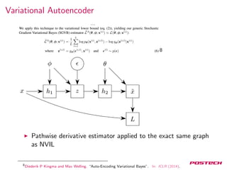
34. Neural Variational Inference
7
Where
L(x, θ, φ) = Eh∼Q(h|x)[logPθ(x, h) − logQφ(h|x)]
Score function estimator
7
Andriy Mnih and Karol Gregor. “Neural Variational Inference and Learning in Belief Networks”. In: ICML
(2014).

35. Variational Autoencoder
8
Pathwise derivative estimator applied to the exact same graph
as NVIL
8
Diederik P Kingma and Max Welling. “Auto-Encoding Variational Bayes”. In: ICLR (2014).

36. DRAW
9
Sequential version of VAE
Same graph as SVG(∞) with (known) deterministic
dynamics(e=state, z=action, L=reward)
Similarly, VAE can be seen as SVG(∞) with 1 timestep and
deterministic dynamics
9
Karol Gregor et al. “DRAW: A Recurrent Neural Network For Image Generation”. In: ICML (2015).

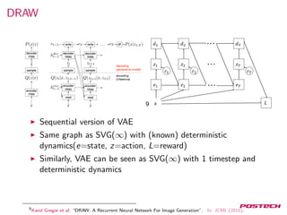
37. GAN
10
Connection to SVG(0) has been established in [10]
Actor has no access to state. Observation is a random choice
between real or fake image. Reward is 1 if real, 0 if fake. D
learns value function of observation. G’s learning signal is D.
10
David Pfau and Oriol Vinyals. “Connecting Generative Adversarial Networks and Actor-Critic Methods”. In:
(2016).

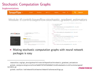
38. Bayes by backprop
11
and our cost function f is:
f (D, θ) = Ew∼q(w|θ)[f (w, θ)]
= Ew∼q(w|θ)[−logp(D|w) + logq(w|θ) − logp(w)]
From the point of view of stochastic computation graphs,
weights and activations are not different
Estimate ELBO gradient of activation with PD estimator:
VAE
Estimate ELBO gradient of weight with PD estimator: Bayes
by Backprop
11
Charles Blundell et al. “Weight Uncertainty in Neural Networks”. In: ICML (2015).

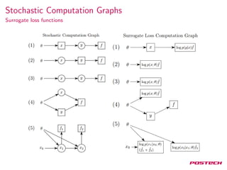
39. Summary
Stochastic computation graphs explain many different
algorithms with one gradient estimator(Theorem 1)
Stochastic computation graphs give us insight into the
behavior of estimators
Stochastic computation graphs reveal equivalencies:
NVIL[7]=Policy gradient[12]
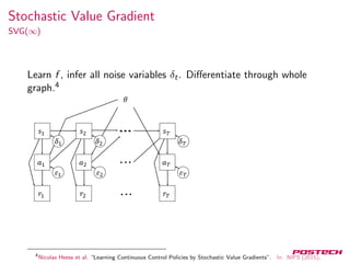
VAE[6]/DRAW[4]=SVG(∞)[5]
GAN[3]=SVG(0)[5]

40. References I
[1] Charles Blundell et al. “Weight Uncertainty in Neural
Networks”. In: ICML (2015).
[2] Michael Fu. “Stochastic Gradient Estimation”. In: (2005).
[3] Ian J. Goodfellow et al. “Generative Adversarial Networks”.
In: NIPS (2014).
[4] Karol Gregor et al. “DRAW: A Recurrent Neural Network
For Image Generation”. In: ICML (2015).
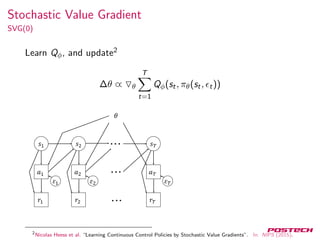
[5] Nicolas Heess et al. “Learning Continuous Control Policies
by Stochastic Value Gradients”. In: NIPS (2015).
[6] Diederik P Kingma and Max Welling. “Auto-Encoding
Variational Bayes”. In: ICLR (2014).
[7] Andriy Mnih and Karol Gregor. “Neural Variational Inference
and Learning in Belief Networks”. In: ICML (2014).

41. References II
[8] David Pfau and Oriol Vinyals. “Connecting Generative
Adversarial Networks and Actor-Critic Methods”. In: (2016).
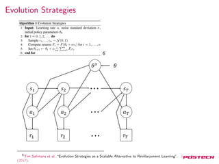
[9] Tim Salimans et al. “Evolution Strategies as a Scalable
Alternative to Reinforcement Learning”. In: arXiv (2017).
[10] John Schulman et al. “Gradient Estimation Using Stochastic
Computation Graphs”. In: NIPS (2015).
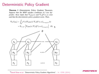
[11] David Silver et al. “Deterministic Policy Gradient
Algorithms”. In: ICML (2014).
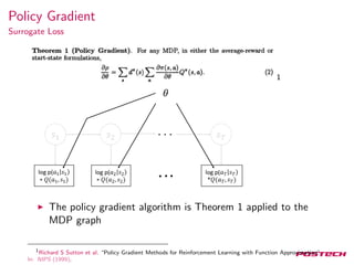
[12] Richard S Sutton et al. “Policy Gradient Methods for
Reinforcement Learning with Function Approximation”. In:
NIPS (1999).

42. Thank You