Download to read offline


![Notation
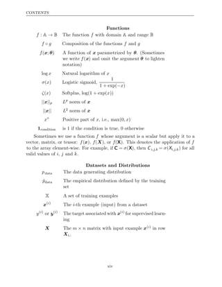
This section provides a concise reference describing the notation used throughout
this book. If you are unfamiliar with any of the corresponding mathematical
concepts, we describe most of these ideas in chapters 2–4.
Numbers and Arrays
a A scalar (integer or real)
a A vector
A A matrix
A A tensor
In Identity matrix with rows and columns
n n
I Identity matrix with dimensionality implied by
context
e( )
i
Standard basis vector [0, . . . , 0, 1,0, . . . ,0] with a
1 at position i
diag( )
a A square, diagonal matrix with diagonal entries
given by a
a A scalar random variable
a A vector-valued random variable
A A matrix-valued random variable
xi](https://image.slidesharecdn.com/deeplearningadaptivecomputationandmachinelearningpdfdrive-230402121325-7c74bca2/85/Deep-learning_-adaptive-computation-and-machine-learning-PDFDrive-pdf-13-320.jpg)
![CONTENTS
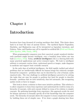
Sets and Graphs
A A set
R The set of real numbers
{ }
0 1
, The set containing 0 and 1
{ }
0 1
, , . . . , n The set of all integers between and
0 n
[ ]
a, b The real interval including and
a b
( ]
a, b The real interval excluding but including
a b
A B
Set subtraction, i.e., the set containing the ele-
ments of that are not in
A B
G A graph
PaG(xi) The parents of xi in G
Indexing
ai Element i of vector a, with indexing starting at 1
a−i All elements of vector except for element
a i
Ai,j Element of matrix
i, j A
Ai,: Row of matrix
i A
A:,i Column of matrix
i A
Ai,j,k Element of a 3-D tensor
( )
i, j, k A
A: :
, ,i 2-D slice of a 3-D tensor
ai Element of the random vector
i a
Linear Algebra Operations
A
Transpose of matrix A
A+
Moore-Penrose pseudoinverse of A
A B
Element-wise (Hadamard) product of and
A B
det( )
A Determinant of A
xii](https://image.slidesharecdn.com/deeplearningadaptivecomputationandmachinelearningpdfdrive-230402121325-7c74bca2/85/Deep-learning_-adaptive-computation-and-machine-learning-PDFDrive-pdf-14-320.jpg)
![CONTENTS
Calculus
dy
dx
Derivative of with respect to
y x
∂y
∂x
Partial derivative of with respect to
y x
∇xy Gradient of with respect to
y x
∇X y Matrix derivatives of with respect to
y X
∇Xy Tensor containing derivatives of y with respect to
X
∂f
∂x
Jacobian matrix J ∈ Rm n
× of f : Rn → Rm
∇2
xf f f
( ) (
x or H )( )
x The Hessian matrix of at input point x
f d
( )
x x Definite integral over the entire domain of x
S
f d
( )
x x x
Definite integral with respect to over the set S
Probability and Information Theory
a b The random variables a and b are independent
⊥
a b c They are conditionally independent given c
⊥ |
P( )
a A probability distribution over a discrete variable
p( )
a A probability distribution over a continuous vari-
able, or over a variable whose type has not been
specified
a Random variable a has distribution
∼ P P
Ex∼P[ ( )] ( ) ( ) ( )
f x or Ef x Expectation of f x with respect to P x
Var( ( ))
f x Variance of under x
f x
( ) P( )
Cov( ( ) ( ))
f x , g x Covariance of and under x
f x
( ) g x
( ) P( )
H( )
x Shannon entropy of the random variable x
DKL( )
P Q
Kullback-Leibler divergence of P and Q
N( ; )
x µ, Σ Gaussian distribution over x with mean µ and
covariance Σ
xiii](https://image.slidesharecdn.com/deeplearningadaptivecomputationandmachinelearningpdfdrive-230402121325-7c74bca2/85/Deep-learning_-adaptive-computation-and-machine-learning-PDFDrive-pdf-15-320.jpg)
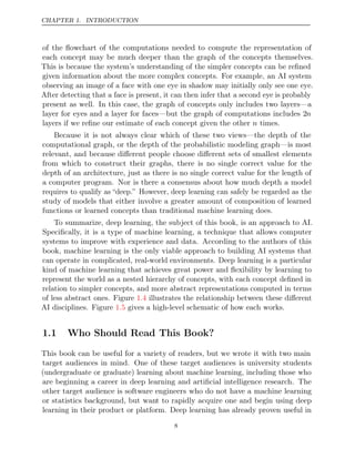
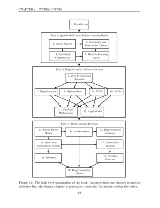
![CHAPTER 1. INTRODUCTION
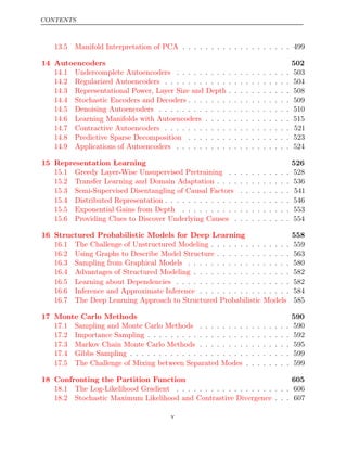
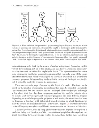
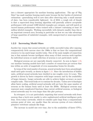
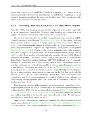
The earliest predecessors of modern deep learning were simple linear models
motivated from a neuroscientific perspective. These models were designed to
take a set of n input values x1, . . . , xn and associate them with an output y.
These models would learn a set of weights w1, . . . , wn and compute their output
f(x w
, ) = x1w1 + · · · + xnwn . This first wave of neural networks research was
known as cybernetics, as illustrated in figure .
1.7
The McCulloch-Pitts Neuron ( , ) was an early model
McCulloch and Pitts 1943
of brain function. This linear model could recognize two different categories of
inputs by testing whether f (x w
, ) is positive or negative. Of course, for the model
to correspond to the desired definition of the categories, the weights needed to be
set correctly. These weights could be set by the human operator. In the 1950s,
the perceptron (Rosenblatt 1958 1962
, , ) became the first model that could learn
the weights defining the categories given examples of inputs from each category.
The adaptive linear element (ADALINE), which dates from about the same
time, simply returned the value of f(x) itself to predict a real number (Widrow
and Hoff 1960
, ), and could also learn to predict these numbers from data.
These simple learning algorithms greatly affected the modern landscape of ma-
chine learning. The training algorithm used to adapt the weights of the ADALINE
was a special case of an algorithm called stochastic gradient descent. Slightly
modified versions of the stochastic gradient descent algorithm remain the dominant
training algorithms for deep learning models today.
Models based on the f(x w
, ) used by the perceptron and ADALINE are called
linear models. These models remain some of the most widely used machine
learning models, though in many cases they are trained in different ways than the
original models were trained.
Linear models have many limitations. Most famously, they cannot learn the
XOR function, where f ([0,1], w) = 1 and f([1,0], w) = 1 but f([1, 1], w) = 0
and f([0, 0], w) = 0. Critics who observed these flaws in linear models caused
a backlash against biologically inspired learning in general (Minsky and Papert,
1969). This was the first major dip in the popularity of neural networks.
Today, neuroscience is regarded as an important source of inspiration for deep
learning researchers, but it is no longer the predominant guide for the field.
The main reason for the diminished role of neuroscience in deep learning
research today is that we simply do not have enough information about the brain
to use it as a guide. To obtain a deep understanding of the actual algorithms used
by the brain, we would need to be able to monitor the activity of (at the very
least) thousands of interconnected neurons simultaneously. Because we are not
able to do this, we are far from understanding even some of the most simple and
15](https://image.slidesharecdn.com/deeplearningadaptivecomputationandmachinelearningpdfdrive-230402121325-7c74bca2/85/Deep-learning_-adaptive-computation-and-machine-learning-PDFDrive-pdf-31-320.jpg)
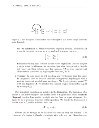
![CHAPTER 2. LINEAR ALGEBRA
define a vector by writing out its elements in the text inline as a row matrix,
then using the transpose operator to turn it into a standard column vector, e.g.,
x = [x1, x2, x3]
.
A scalar can be thought of as a matrix with only a single entry. From this, we
can see that a scalar is its own transpose: a a
= .
We can add matrices to each other, as long as they have the same shape, just
by adding their corresponding elements: where
C A B
= + Ci,j = Ai,j + Bi,j.
We can also add a scalar to a matrix or multiply a matrix by a scalar, just
by performing that operation on each element of a matrix: D = a · B + c where
Di,j = a B
· i,j + c.
In the context of deep learning, we also use some less conventional notation.
We allow the addition of matrix and a vector, yielding another matrix: C = A +b,
where Ci,j = Ai,j + bj. In other words, the vector b is added to each row of the
matrix. This shorthand eliminates the need to define a matrix with b copied into
each row before doing the addition. This implicit copying of b to many locations
is called .
broadcasting
2.2 Multiplying Matrices and Vectors
One of the most important operations involving matrices is multiplication of two
matrices. The matrix product of matrices A and B is a third matrix C. In
order for this product to be defined, A must have the same number of columns as
B has rows. If A is of shape m n
× and B is of shape n p
× , then C is of shape
m p
× . We can write the matrix product just by placing two or more matrices
together, e.g.
C AB
= . (2.4)
The product operation is defined by
Ci,j =
k
Ai,kBk,j. (2.5)
Note that the standard product of two matrices is just a matrix containing
not
the product of the individual elements. Such an operation exists and is called the
element-wise product Hadamard product
or , and is denoted as .
A B
The dot product between two vectors x and y of the same dimensionality
is the matrix product xy. We can think of the matrix product C = AB as
computing Ci,j as the dot product between row of and column of .
i A j B
34](https://image.slidesharecdn.com/deeplearningadaptivecomputationandmachinelearningpdfdrive-230402121325-7c74bca2/85/Deep-learning_-adaptive-computation-and-machine-learning-PDFDrive-pdf-50-320.jpg)
![CHAPTER 2. LINEAR ALGEBRA
all i = j. We have already seen one example of a diagonal matrix: the identity
matrix, where all of the diagonal entries are 1. We write diag(v) to denote a square
diagonal matrix whose diagonal entries are given by the entries of the vector v.
Diagonal matrices are of interest in part because multiplying by a diagonal matrix
is very computationally efficient. To compute diag(v)x, we only need to scale each
element xi by vi. In other words, diag(v)x = v x
. Inverting a square diagonal
matrix is also efficient. The inverse exists only if every diagonal entry is nonzero,
and in that case, diag(v)−1 = diag([1/v1, . . . ,1/vn ]). In many cases, we may
derive some very general machine learning algorithm in terms of arbitrary matrices,
but obtain a less expensive (and less descriptive) algorithm by restricting some
matrices to be diagonal.
Not all diagonal matrices need be square. It is possible to construct a rectangular
diagonal matrix. Non-square diagonal matrices do not have inverses but it is still
possible to multiply by them cheaply. For a non-square diagonal matrix D, the
product Dx will involve scaling each element of x, and either concatenating some
zeros to the result if D is taller than it is wide, or discarding some of the last
elements of the vector if is wider than it is tall.
D
A matrix is any matrix that is equal to its own transpose:
symmetric
A A
=
. (2.35)
Symmetric matrices often arise when the entries are generated by some function of
two arguments that does not depend on the order of the arguments. For example,
if A is a matrix of distance measurements, with Ai,j giving the distance from point
i to point , then
j Ai,j = Aj,i because distance functions are symmetric.
A is a vector with :
unit vector unit norm
|| ||
x 2 = 1. (2.36)
A vector x and a vector y are orthogonal to each other if x
y = 0. If both
vectors have nonzero norm, this means that they are at a 90 degree angle to each
other. In Rn , at most n vectors may be mutually orthogonal with nonzero norm.
If the vectors are not only orthogonal but also have unit norm, we call them
orthonormal.
An orthogonal matrix is a square matrix whose rows are mutually orthonor-
mal and whose columns are mutually orthonormal:
A
A AA
=
= I. (2.37)
41](https://image.slidesharecdn.com/deeplearningadaptivecomputationandmachinelearningpdfdrive-230402121325-7c74bca2/85/Deep-learning_-adaptive-computation-and-machine-learning-PDFDrive-pdf-57-320.jpg)
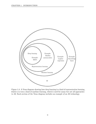
![CHAPTER 2. LINEAR ALGEBRA
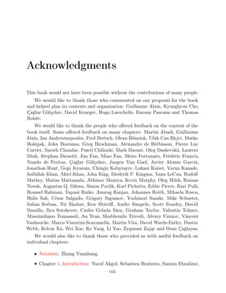
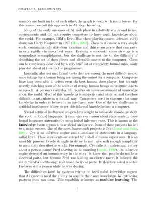
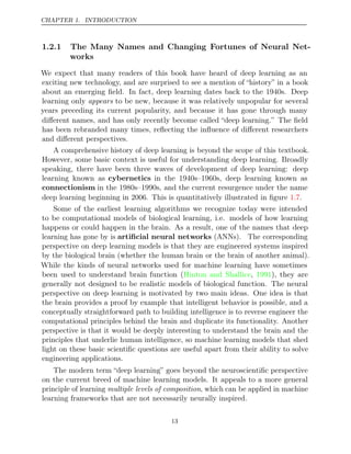
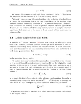
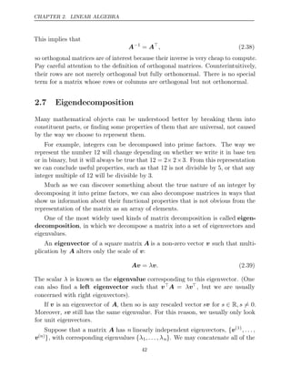
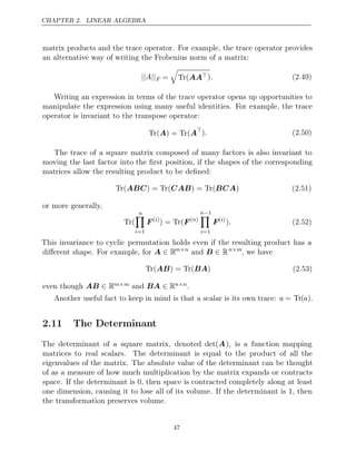
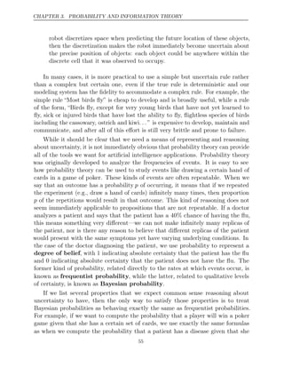
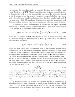
Figure 2.3: An example of the effect of eigenvectors and eigenvalues. Here, we have
a matrix A with two orthonormal eigenvectors, v(1)
with eigenvalue λ1 and v(2)
with
eigenvalue λ2. (Left)We plot the set of all unit vectors u ∈ R2
as a unit circle. (Right)We
plot the set of all points Au. By observing the way that A distorts the unit circle, we
can see that it scales space in direction v( )
i
by λi.
eigenvectors to form a matrix V with one eigenvector per column: V = [v(1), . . . ,
v( )
n ]. Likewise, we can concatenate the eigenvalues to form a vector λ = [λ1, . . . ,
λn ]. The of is then given by
eigendecomposition A
A V λ V
= diag( ) −1
. (2.40)
We have seen that constructing matrices with specific eigenvalues and eigenvec-
tors allows us to stretch space in desired directions. However, we often want to
decompose matrices into their eigenvalues and eigenvectors. Doing so can help
us to analyze certain properties of the matrix, much as decomposing an integer
into its prime factors can help us understand the behavior of that integer.
Not every matrix can be decomposed into eigenvalues and eigenvectors. In some
43](https://image.slidesharecdn.com/deeplearningadaptivecomputationandmachinelearningpdfdrive-230402121325-7c74bca2/85/Deep-learning_-adaptive-computation-and-machine-learning-PDFDrive-pdf-59-320.jpg)
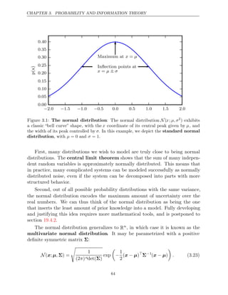
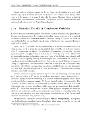
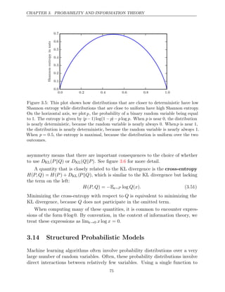
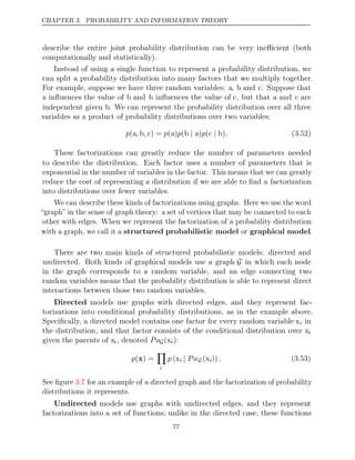
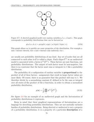
![CHAPTER 3. PROBABILITY AND INFORMATION THEORY
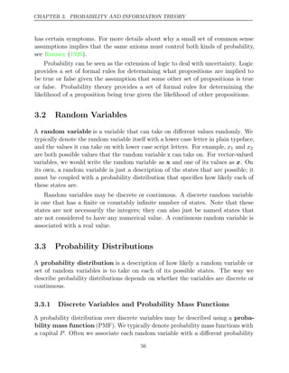
3.3.2 Continuous Variables and Probability Density Functions
When working with continuous random variables, we describe probability distri-
butions using a probability density function (PDF) rather than a probability
mass function. To be a probability density function, a function p must satisfy the
following properties:
• The domain of must be the set of all possible states of x.
p
• ∀ ∈ ≥ ≤
x x,p x
( ) 0 ( )
. p
Note that we do not require x 1.
•
p x dx
( ) = 1.
A probability density function p(x) does not give the probability of a specific
state directly, instead the probability of landing inside an infinitesimal region with
volume is given by .
δx p x δx
( )
We can integrate the density function to find the actual probability mass of a
set of points. Specifically, the probability that x lies in some set S is given by the
integral of p(x) over that set. In the univariate example, the probability that x
lies in the interval is given by
[ ]
a, b
[ ]
a,b p x dx
( ) .
For an example of a probability density function corresponding to a specific
probability density over a continuous random variable, consider a uniform distribu-
tion on an interval of the real numbers. We can do this with a function u(x;a,b),
where a and b are the endpoints of the interval, with b > a. The “;” notation means
“parametrized by”; we consider x to be the argument of the function, while a and
b are parameters that define the function. To ensure that there is no probability
mass outside the interval, we say u(x;a,b) = 0 for all x ∈ [a,b] [
. Within a,b],
u x a, b
( ; ) = 1
b a
− . We can see that this is nonnegative everywhere. Additionally, it
integrates to 1. We often denote that x follows the uniform distribution on [a,b]
by writing x .
∼ U a,b
( )
3.4 Marginal Probability
Sometimes we know the probability distribution over a set of variables and we want
to know the probability distribution over just a subset of them. The probability
distribution over the subset is known as the distribution.
marginal probability
For example, suppose we have discrete random variables x and y, and we know
P ,
(x y . We can find x with the :
) P( ) sum rule
∀ ∈
x x x
,P ( = ) =
x
y
P x, y .
( =
x y = ) (3.3)
58](https://image.slidesharecdn.com/deeplearningadaptivecomputationandmachinelearningpdfdrive-230402121325-7c74bca2/85/Deep-learning_-adaptive-computation-and-machine-learning-PDFDrive-pdf-74-320.jpg)
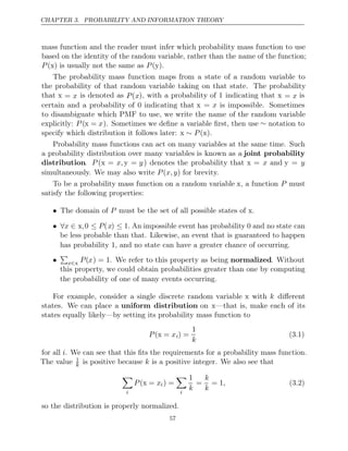
![CHAPTER 3. PROBABILITY AND INFORMATION THEORY
For example, applying the definition twice, we get
P , , P , P ,
(a b c) = (a b
| c) (b c)
P , P P
(b c) = ( )
b c
| ( )
c
P , , P , P P .
(a b c) = (a b
| c) ( )
b c
| ( )
c
3.7 Independence and Conditional Independence
Two random variables x and y are independent if their probability distribution
can be expressed as a product of two factors, one involving only x and one involving
only y:
∀ ∈ ∈
x x,y y x y x y (3.7)
, p( = x, = ) = (
y p = ) (
x p = )
y .
Two random variables x and y areconditionally independent given a random
variable z if the conditional probability distribution over x and y factorizes in this
way for every value of z:
∀ ∈ ∈ ∈ | | |
x x,y y,z z x y
, p( = x, = y z x
= ) = (
z p = x z y
= ) (
z p = y z = )
z .
(3.8)
We can denote independence and conditional independence with compact
notation: x y
⊥ means that x and y are independent, while x y z
⊥ | means that x
and y are conditionally independent given z.
3.8 Expectation, Variance and Covariance
The expectation or expected value of some function f(x) with respect to a
probability distribution P (x) is the average or mean value that f takes on when x
is drawn from . For discrete variables this can be computed with a summation:
P
Ex∼P [ ( )] =
f x
x
P x f x ,
( ) ( ) (3.9)
while for continuous variables, it is computed with an integral:
Ex∼p[ ( )] =
f x
p x f x dx.
( ) ( ) (3.10)
60](https://image.slidesharecdn.com/deeplearningadaptivecomputationandmachinelearningpdfdrive-230402121325-7c74bca2/85/Deep-learning_-adaptive-computation-and-machine-learning-PDFDrive-pdf-76-320.jpg)
![CHAPTER 3. PROBABILITY AND INFORMATION THEORY
When the identity of the distribution is clear from the context, we may simply
write the name of the random variable that the expectation is over, as in Ex[f(x)].
If it is clear which random variable the expectation is over, we may omit the
subscript entirely, as in E[f(x)]. By default, we can assume that E[·] averages over
the values of all the random variables inside the brackets. Likewise, when there is
no ambiguity, we may omit the square brackets.
Expectations are linear, for example,
Ex[ ( ) + ( )] =
αf x βg x αEx[ ( )] +
f x βEx[ ( )]
g x , (3.11)
when and are not dependent on .
α β x
The variance gives a measure of how much the values of a function of a random
variable x vary as we sample different values of x from its probability distribution:
Var( ( )) =
f x E
( ( ) [ ( )])
f x − E f x 2
. (3.12)
When the variance is low, the values of f(x) cluster near their expected value. The
square root of the variance is known as the .
standard deviation
The covariance gives some sense of how much two values are linearly related
to each other, as well as the scale of these variables:
Cov( ( ) ( )) = [( ( ) [ ( )])( ( ) [ ( )])]
f x , g y E f x − E f x g y − E g y . (3.13)
High absolute values of the covariance mean that the values change very much
and are both far from their respective means at the same time. If the sign of the
covariance is positive, then both variables tend to take on relatively high values
simultaneously. If the sign of the covariance is negative, then one variable tends to
take on a relatively high value at the times that the other takes on a relatively
low value and vice versa. Other measures such as correlation normalize the
contribution of each variable in order to measure only how much the variables are
related, rather than also being affected by the scale of the separate variables.
The notions of covariance and dependence are related, but are in fact distinct
concepts. They are related because two variables that are independent have zero
covariance, and two variables that have non-zero covariance are dependent. How-
ever, independence is a distinct property from covariance. For two variables to have
zero covariance, there must be no linear dependence between them. Independence
is a stronger requirement than zero covariance, because independence also excludes
nonlinear relationships. It is possible for two variables to be dependent but have
zero covariance. For example, suppose we first sample a real number x from a
uniform distribution over the interval [−1, 1]. We next sample a random variable
61](https://image.slidesharecdn.com/deeplearningadaptivecomputationandmachinelearningpdfdrive-230402121325-7c74bca2/85/Deep-learning_-adaptive-computation-and-machine-learning-PDFDrive-pdf-77-320.jpg)
![CHAPTER 3. PROBABILITY AND INFORMATION THEORY
s. With probability 1
2 , we choose the value of s to be . Otherwise, we choose
1
the value of s to be −1. We can then generate a random variable y by assigning
y = sx. Clearly, x and y are not independent, because x completely determines
the magnitude of . However,
y Cov( ) = 0
x, y .
The covariance matrix of a random vector x ∈ Rn is an n n
× matrix, such
that
Cov( )
x i,j = Cov(xi,xj). (3.14)
The diagonal elements of the covariance give the variance:
Cov(xi,xi) = Var(xi ). (3.15)
3.9 Common Probability Distributions
Several simple probability distributions are useful in many contexts in machine
learning.
3.9.1 Bernoulli Distribution
The Bernoulli distribution is a distribution over a single binary random variable.
It is controlled by a single parameter φ ∈ [0,1], which gives the probability of the
random variable being equal to 1. It has the following properties:
P φ
( = 1) =
x (3.16)
P φ
( = 0) = 1
x − (3.17)
P x φ
( =
x ) = x
(1 )
− φ 1−x
(3.18)
Ex[ ] =
x φ (3.19)
Varx( ) = (1 )
x φ − φ (3.20)
3.9.2 Multinoulli Distribution
The multinoulli or categorical distribution is a distribution over a single discrete
variable with k different states, where k is finite.1
The multinoulli distribution is
1
“Multinoulli” is a term that was recently coined by Gustavo Lacerdo and popularized by
Murphy 2012
( ). The multinoulli distribution is a special case of the multinomial distribution.
A multinomial distribution is the distribution over vectors in {0,. . ., n}k
representing how many
times each of the k categories is visited when n samples are drawn from a multinoulli distribution.
Many texts use the term “multinomial” to refer to multinoulli distributions without clarifying
that they refer only to the case.
n = 1
62](https://image.slidesharecdn.com/deeplearningadaptivecomputationandmachinelearningpdfdrive-230402121325-7c74bca2/85/Deep-learning_-adaptive-computation-and-machine-learning-PDFDrive-pdf-78-320.jpg)
![CHAPTER 3. PROBABILITY AND INFORMATION THEORY
parametrized by a vector p ∈ [0,1]k−1
, where pi gives the probability of the i-th
state. The final, k-th state’s probability is given by 1− 1
p. Note that we must
constrain 1
p ≤ 1. Multinoulli distributions are often used to refer to distributions
over categories of objects, so we do not usually assume that state 1 has numerical
value 1, etc. For this reason, we do not usually need to compute the expectation
or variance of multinoulli-distributed random variables.
The Bernoulli and multinoulli distributions are sufficient to describe any distri-
bution over their domain. They are able to describe any distribution over their
domain not so much because they are particularly powerful but rather because
their domain is simple; they model discrete variables for which it is feasible to
enumerate all of the states. When dealing with continuous variables, there are
uncountably many states, so any distribution described by a small number of
parameters must impose strict limits on the distribution.
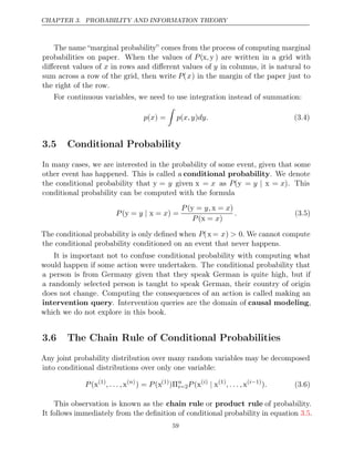
3.9.3 Gaussian Distribution
The most commonly used distribution over real numbers is the normal distribu-
tion, also known as the :
Gaussian distribution
N ( ;
x µ, σ2
) =
1
2πσ2
exp
−
1
2σ2
( )
x µ
− 2
. (3.21)
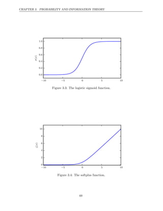
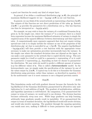
See figure for a plot of the density function.
3.1
The two parameters µ ∈ R and σ ∈ (0,∞) control the normal distribution.
The parameter µ gives the coordinate of the central peak. This is also the mean of
the distribution: E[x] = µ. The standard deviation of the distribution is given by
σ, and the variance by σ2.
When we evaluate the PDF, we need to square and invert σ. When we need to
frequently evaluate the PDF with different parameter values, a more efficient way
of parametrizing the distribution is to use a parameter β ∈ (0,∞) to control the
precision or inverse variance of the distribution:
N( ;
x µ, β−1
) =
β
2π
exp
−
1
2
β x µ
( − )2
. (3.22)
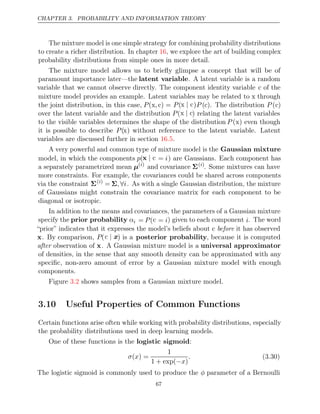
Normal distributions are a sensible choice for many applications. In the absence
of prior knowledge about what form a distribution over the real numbers should
take, the normal distribution is a good default choice for two major reasons.
63](https://image.slidesharecdn.com/deeplearningadaptivecomputationandmachinelearningpdfdrive-230402121325-7c74bca2/85/Deep-learning_-adaptive-computation-and-machine-learning-PDFDrive-pdf-79-320.jpg)
![CHAPTER 3. PROBABILITY AND INFORMATION THEORY
measure zero. Because the exceptions occupy a negligible amount of space, they
can be safely ignored for many applications. Some important results in probability
theory hold for all discrete values but only hold “almost everywhere” for continuous
values.
Another technical detail of continuous variables relates to handling continuous
random variables that are deterministic functions of one another. Suppose we have
two random variables, x and y, such that y = g(x), where g is an invertible, con-
tinuous, differentiable transformation. One might expect that py (y) = px(g−1
(y)).
This is actually not the case.
As a simple example, suppose we have scalar random variables x and y. Suppose
y = x
2 and x ∼ U(0, 1). If we use the rule py(y) = px (2y) then py will be 0
everywhere except the interval [0, 1
2] 1
, and it will be on this interval. This means
py( ) =
y dy
1
2
, (3.43)
which violates the definition of a probability distribution. This is a common mistake.
The problem with this approach is that it fails to account for the distortion of
space introduced by the function g. Recall that the probability of x lying in an
infinitesimally small region with volume δx is given by p(x)δx. Since g can expand
or contract space, the infinitesimal volume surrounding x in x space may have
different volume in space.
y
To see how to correct the problem, we return to the scalar case. We need to
preserve the property
|py( ( )) =
g x dy| |px( )
x dx .
| (3.44)
Solving from this, we obtain
py( ) =
y px (g−1
( ))
y
∂x
∂y
(3.45)
or equivalently
px( ) =
x py( ( ))
g x
∂g x
( )
∂x
. (3.46)
In higher dimensions, the derivative generalizes to the determinant of the Jacobian
matrix—the matrix with Ji,j = ∂xi
∂yj
. Thus, for real-valued vectors and ,
x y
px( ) =
x py( ( ))
g x
det
∂g( )
x
∂x
. (3.47)
72](https://image.slidesharecdn.com/deeplearningadaptivecomputationandmachinelearningpdfdrive-230402121325-7c74bca2/85/Deep-learning_-adaptive-computation-and-machine-learning-PDFDrive-pdf-88-320.jpg)
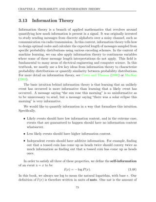
![CHAPTER 3. PROBABILITY AND INFORMATION THEORY
information gained by observing an event of probability 1
e. Other texts use base-2
logarithms and units called bits or shannons; information measured in bits is
just a rescaling of information measured in nats.
When x is continuous, we use the same definition of information by analogy,
but some of the properties from the discrete case are lost. For example, an event
with unit density still has zero information, despite not being an event that is
guaranteed to occur.
Self-information deals only with a single outcome. We can quantify the amount
of uncertainty in an entire probability distribution using the Shannon entropy:
H( ) =
x Ex∼P [ ( )] =
I x −Ex∼P [log ( )]
P x . (3.49)
also denoted H(P). In other words, the Shannon entropy of a distribution is the
expected amount of information in an event drawn from that distribution. It gives
a lower bound on the number of bits (if the logarithm is base 2, otherwise the units
are different) needed on average to encode symbols drawn from a distribution P.
Distributions that are nearly deterministic (where the outcome is nearly certain)
have low entropy; distributions that are closer to uniform have high entropy. See
figure for a demonstration. When
3.5 x is continuous, the Shannon entropy is
known as the differential entropy.
If we have two separate probability distributions P (x) and Q(x) over the same
random variable x, we can measure how different these two distributions are using
the Kullback-Leibler (KL) divergence:
DKL( ) =
P Q
Ex∼P
log
P x
( )
Q x
( )
= Ex∼P [log ( ) log ( )]
P x − Q x . (3.50)
In the case of discrete variables, it is the extra amount of information (measured
in bits if we use the base logarithm, but in machine learning we usually use nats
2
and the natural logarithm) needed to send a message containing symbols drawn
from probability distribution P, when we use a code that was designed to minimize
the length of messages drawn from probability distribution .
Q
The KL divergence has many useful properties, most notably that it is non-
negative. The KL divergence is 0 if and only if P and Q are the same distribution in
the case of discrete variables, or equal “almost everywhere” in the case of continuous
variables. Because the KL divergence is non-negative and measures the difference
between two distributions, it is often conceptualized as measuring some sort of
distance between these distributions. However, it is not a true distance measure
because it is not symmetric: DKL(P Q
) = DKL(Q P
) for some P and Q. This
74](https://image.slidesharecdn.com/deeplearningadaptivecomputationandmachinelearningpdfdrive-230402121325-7c74bca2/85/Deep-learning_-adaptive-computation-and-machine-learning-PDFDrive-pdf-90-320.jpg)

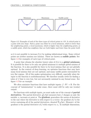
![CHAPTER 4. NUMERICAL COMPUTATION
− − −
30 20 10 0 10 20
x1
−30
−20
−10
0
10
20
x
2
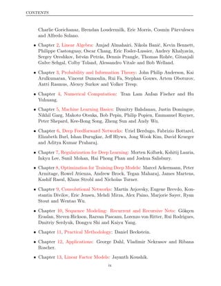
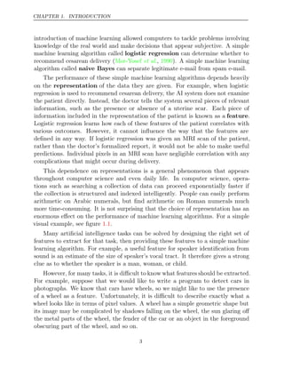
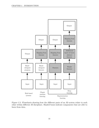
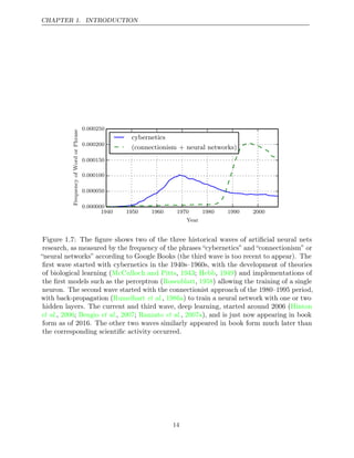
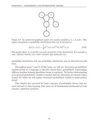
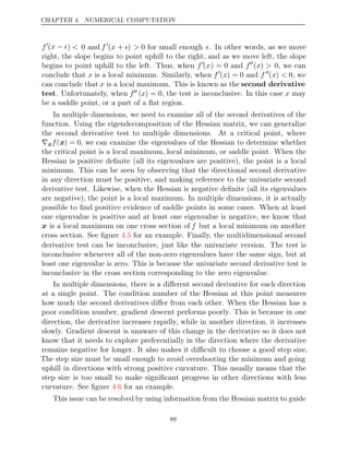
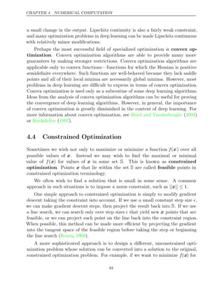
Figure 4.6: Gradient descent fails to exploit the curvature information contained in the
Hessian matrix. Here we use gradient descent to minimize a quadratic functionf(x) whose
Hessian matrix has condition number 5. This means that the direction of most curvature
has five times more curvature than the direction of least curvature. In this case, the most
curvature is in the direction [1, 1] and the least curvature is in the direction [1, −1]. The
red lines indicate the path followed by gradient descent. This very elongated quadratic
function resembles a long canyon. Gradient descent wastes time repeatedly descending
canyon walls, because they are the steepest feature. Because the step size is somewhat
too large, it has a tendency to overshoot the bottom of the function and thus needs to
descend the opposite canyon wall on the next iteration. The large positive eigenvalue
of the Hessian corresponding to the eigenvector pointed in this direction indicates that
this directional derivative is rapidly increasing, so an optimization algorithm based on
the Hessian could predict that the steepest direction is not actually a promising search
direction in this context.
91](https://image.slidesharecdn.com/deeplearningadaptivecomputationandmachinelearningpdfdrive-230402121325-7c74bca2/85/Deep-learning_-adaptive-computation-and-machine-learning-PDFDrive-pdf-107-320.jpg)
![CHAPTER 4. NUMERICAL COMPUTATION
x ∈ R2
with x constrained to have exactly unit L2
norm, we can instead minimize
g(θ) = f ([cos sin
θ, θ]
) with respect to θ, then return [cos sin
θ, θ] as the solution
to the original problem. This approach requires creativity; the transformation
between optimization problems must be designed specifically for each case we
encounter.
The Karush–Kuhn–Tucker (KKT) approach1 provides a very general so-
lution to constrained optimization. With the KKT approach, we introduce a
new function called the generalized Lagrangian or generalized Lagrange
function.
To define the Lagrangian, we first need to describe S in terms of equations
and inequalities. We want a description of S in terms of m functions g( )
i and n
functions h( )
j so that S = { | ∀
x i, g( )
i (x) = 0 and ∀j, h( )
j (x) ≤ 0}. The equations
involving g( )
i are called the equality constraints and the inequalities involving
h( )
j
are called .
inequality constraints
We introduce new variables λi andαj for each constraint, these are called the
KKT multipliers. The generalized Lagrangian is then defined as
L , , f
(x λ α) = ( ) +
x
i
λi g( )
i
( ) +
x
j
αjh( )
j
( )
x . (4.14)
We can now solve a constrained minimization problem using unconstrained
optimization of the generalized Lagrangian. Observe that, so long as at least one
feasible point exists and is not permitted to have value , then
f( )
x ∞
min
x
max
λ
max
α α
, ≥0
L , , .
(x λ α) (4.15)
has the same optimal objective function value and set of optimal points as
x
min
x∈S
f .
( )
x (4.16)
This follows because any time the constraints are satisfied,
max
λ
max
α α
, ≥0
L , , f ,
(x λ α) = ( )
x (4.17)
while any time a constraint is violated,
max
λ
max
α α
, ≥0
L , , .
(x λ α) = ∞ (4.18)
1
The KKT approach generalizes the method of Lagrange multipliers which allows equality
constraints but not inequality constraints.
94](https://image.slidesharecdn.com/deeplearningadaptivecomputationandmachinelearningpdfdrive-230402121325-7c74bca2/85/Deep-learning_-adaptive-computation-and-machine-learning-PDFDrive-pdf-110-320.jpg)
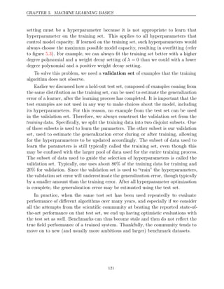
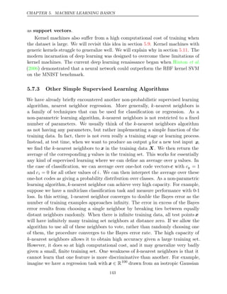
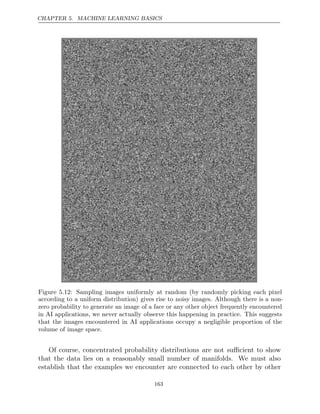
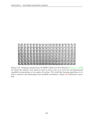
![CHAPTER 5. MACHINE LEARNING BASICS
where the expectation is over the data (seen as samples from a random variable)
and θ is the true underlying value of θ used to define the data generating distri-
bution. An estimator θ̂m is said to be unbiased if bias(θ̂m) = 0, which implies
that E(θ̂m) = θ. An estimator ˆ
θm is said to be asymptotically unbiased if
limm→∞ bias(θ̂m) = 0, which implies that limm→∞ E(ˆ
θm) = θ.
Example: Bernoulli Distribution Consider a set of samples {x(1)
, . . . , x( )
m
}
that are independently and identically distributed according to a Bernoulli distri-
bution with mean :
θ
P x
( ( )
i
; ) =
θ θx ( )
i
(1 )
− θ (1−x( )
i )
. (5.21)
A common estimator for the θ parameter of this distribution is the mean of the
training samples:
θ̂m =
1
m
m
i=1
x( )
i
. (5.22)
To determine whether this estimator is biased, we can substitute equation 5.22
into equation :
5.20
bias(θ̂m) = [
E ˆ
θm] − θ (5.23)
= E
1
m
m
i=1
x( )
i
− θ (5.24)
=
1
m
m
i=1
E
x( )
i
− θ (5.25)
=
1
m
m
i=1
1
x( )
i =0
x( )
i
θx ( )
i
(1 )
− θ (1−x( )
i )
− θ (5.26)
=
1
m
m
i=1
( )
θ − θ (5.27)
= = 0
θ θ
− (5.28)
Since bias(θ̂) = 0, we say that our estimator θ̂ is unbiased.
Example: Gaussian Distribution Estimator of the Mean Now, consider
a set of samples {x(1), . . . , x( )
m } that are independently and identically distributed
according to a Gaussian distribution p(x( )
i ) = N (x( )
i ; µ, σ2), where i ∈ {1, . . . , m}.
125](https://image.slidesharecdn.com/deeplearningadaptivecomputationandmachinelearningpdfdrive-230402121325-7c74bca2/85/Deep-learning_-adaptive-computation-and-machine-learning-PDFDrive-pdf-141-320.jpg)
![CHAPTER 5. MACHINE LEARNING BASICS
Recall that the Gaussian probability density function is given by
p x
( ( )
i
; µ, σ2
) =
1
√
2πσ2
exp
−
1
2
(x( )
i − µ)2
σ2
. (5.29)
A common estimator of the Gaussian mean parameter is known as the sample
mean:
µ̂m =
1
m
m
i=1
x( )
i
(5.30)
To determine the bias of the sample mean, we are again interested in calculating
its expectation:
bias(µ̂m ) = [ˆ
E µm] − µ (5.31)
= E
1
m
m
i=1
x( )
i
− µ (5.32)
=
1
m
m
i=1
E
x( )
i
− µ (5.33)
=
1
m
m
i=1
µ
− µ (5.34)
= = 0
µ µ
− (5.35)
Thus we find that the sample mean is an unbiased estimator of Gaussian mean
parameter.
Example: Estimators of the Variance of a Gaussian Distribution As an
example, we compare two different estimators of the variance parameter σ2 of a
Gaussian distribution. We are interested in knowing if either estimator is biased.
The first estimator of σ2
we consider is known as the sample variance:
σ̂2
m =
1
m
m
i=1
x( )
i
− µ̂m
2
, (5.36)
where µ̂m is the sample mean, defined above. More formally, we are interested in
computing
bias(σ̂2
m) = [ˆ
E σ2
m] − σ2
(5.37)
126](https://image.slidesharecdn.com/deeplearningadaptivecomputationandmachinelearningpdfdrive-230402121325-7c74bca2/85/Deep-learning_-adaptive-computation-and-machine-learning-PDFDrive-pdf-142-320.jpg)
![CHAPTER 5. MACHINE LEARNING BASICS
We begin by evaluating the term E[σ̂2
m ]:
E[σ̂2
m] =E
1
m
m
i=1
x( )
i − µ̂m
2
(5.38)
=
m − 1
m
σ2
(5.39)
Returning to equation , we conclude that the bias of
5.37 σ̂2
m is −σ2/m. Therefore,
the sample variance is a biased estimator.
The unbiased sample variance estimator
σ̃2
m =
1
m − 1
m
i=1
x( )
i
− µ̂m
2
(5.40)
provides an alternative approach. As the name suggests this estimator is unbiased.
That is, we find that E[σ̃2
m] = σ2
:
E[σ̃2
m] = E
1
m − 1
m
i=1
x( )
i − µ̂m
2
(5.41)
=
m
m − 1
E[σ̂2
m ] (5.42)
=
m
m − 1
m − 1
m
σ2
(5.43)
= σ2
. (5.44)
We have two estimators: one is biased and the other is not. While unbiased
estimators are clearly desirable, they are not always the “best” estimators. As we
will see we often use biased estimators that possess other important properties.
5.4.3 Variance and Standard Error
Another property of the estimator that we might want to consider is how much
we expect it to vary as a function of the data sample. Just as we computed the
expectation of the estimator to determine its bias, we can compute its variance.
The variance of an estimator is simply the variance
Var(ˆ
θ) (5.45)
where the random variable is the training set. Alternately, the square root of the
variance is called the , denoted
standard error SE(θ̂).
127](https://image.slidesharecdn.com/deeplearningadaptivecomputationandmachinelearningpdfdrive-230402121325-7c74bca2/85/Deep-learning_-adaptive-computation-and-machine-learning-PDFDrive-pdf-143-320.jpg)
![CHAPTER 5. MACHINE LEARNING BASICS
Example: Bernoulli Distribution We once again consider a set of samples
{x(1)
, . . . , x( )
m
} drawn independently and identically from a Bernoulli distribution
(recall P(x( )
i
;θ) = θx( )
i
(1 − θ)(1−x( )
i )
). This time we are interested in computing
the variance of the estimator θ̂m = 1
m
m
i=1 x( )
i
.
Var
θ̂m
= Var
1
m
m
i=1
x( )
i
(5.48)
=
1
m2
m
i=1
Var
x( )
i
(5.49)
=
1
m2
m
i=1
θ θ
(1 − ) (5.50)
=
1
m2
mθ θ
(1 − ) (5.51)
=
1
m
θ θ
(1 − ) (5.52)
The variance of the estimator decreases as a function of m, the number of examples
in the dataset. This is a common property of popular estimators that we will
return to when we discuss consistency (see section ).
5.4.5
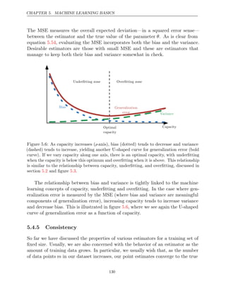
5.4.4 Trading off Bias and Variance to Minimize Mean Squared
Error
Bias and variance measure two different sources of error in an estimator. Bias
measures the expected deviation from the true value of the function or parameter.
Variance on the other hand, provides a measure of the deviation from the expected
estimator value that any particular sampling of the data is likely to cause.
What happens when we are given a choice between two estimators, one with
more bias and one with more variance? How do we choose between them? For
example, imagine that we are interested in approximating the function shown in
figure and we are only offered the choice between a model with large bias and
5.2
one that suffers from large variance. How do we choose between them?
The most common way to negotiate this trade-off is to use cross-validation.
Empirically, cross-validation is highly successful on many real-world tasks. Alter-
natively, we can also compare the mean squared error (MSE) of the estimates:
MSE = [(
E θ̂m − θ)2
] (5.53)
= Bias(θ̂m)2
+ Var(ˆ
θm ) (5.54)
129](https://image.slidesharecdn.com/deeplearningadaptivecomputationandmachinelearningpdfdrive-230402121325-7c74bca2/85/Deep-learning_-adaptive-computation-and-machine-learning-PDFDrive-pdf-145-320.jpg)
![CHAPTER 5. MACHINE LEARNING BASICS
This product over many probabilities can be inconvenient for a variety of reasons.
For example, it is prone to numerical underflow. To obtain a more convenient
but equivalent optimization problem, we observe that taking the logarithm of the
likelihood does not change its arg max but does conveniently transform a product
into a sum:
θML = arg max
θ
m
i=1
log pmodel(x( )
i
; )
θ . (5.58)
Because the arg max does not change when we rescale the cost function, we can
divide by m to obtain a version of the criterion that is expressed as an expectation
with respect to the empirical distribution p̂data defined by the training data:
θML = arg max
θ
Ex∼p̂data
log pmodel ( ; )
x θ . (5.59)
One way to interpret maximum likelihood estimation is to view it as minimizing
the dissimilarity between the empirical distribution p̂data defined by the training
set and the model distribution, with the degree of dissimilarity between the two
measured by the KL divergence. The KL divergence is given by
DKL (p̂data pmodel) = Ex∼p̂data
[log p̂data ( ) log
x − pmodel( )]
x . (5.60)
The term on the left is a function only of the data generating process, not the
model. This means when we train the model to minimize the KL divergence, we
need only minimize
− Ex∼p̂data [log pmodel( )]
x (5.61)
which is of course the same as the maximization in equation .
5.59
Minimizing this KL divergence corresponds exactly to minimizing the cross-
entropy between the distributions. Many authors use the term “cross-entropy” to
identify specifically the negative log-likelihood of a Bernoulli or softmax distribution,
but that is a misnomer. Any loss consisting of a negative log-likelihood is a cross-
entropy between the empirical distribution defined by the training set and the
probability distribution defined by model. For example, mean squared error is the
cross-entropy between the empirical distribution and a Gaussian model.
We can thus see maximum likelihood as an attempt to make the model dis-
tribution match the empirical distribution p̂data. Ideally, we would like to match
the true data generating distribution pdata, but we have no direct access to this
distribution.
While the optimal θ is the same regardless of whether we are maximizing the
likelihood or minimizing the KL divergence, the values of the objective functions
132](https://image.slidesharecdn.com/deeplearningadaptivecomputationandmachinelearningpdfdrive-230402121325-7c74bca2/85/Deep-learning_-adaptive-computation-and-machine-learning-PDFDrive-pdf-148-320.jpg)

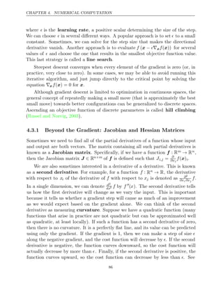
![CHAPTER 5. MACHINE LEARNING BASICS
− −
20 10 0 10 20
x1
−20
−10
0
10
20
x
2
− −
20 10 0 10 20
z1
−20
−10
0
10
20
z
2
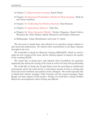
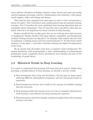
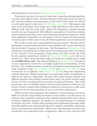
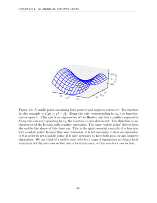
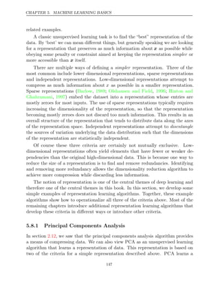
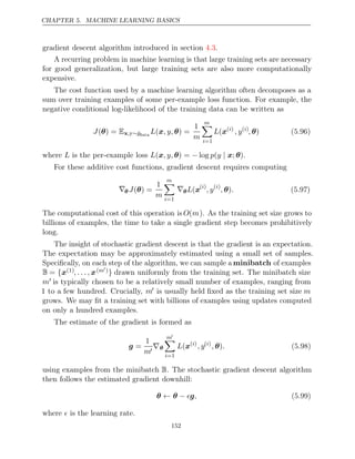
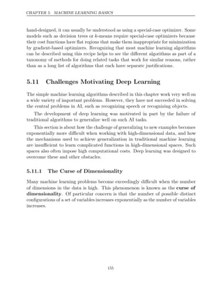
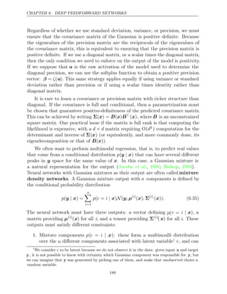
Figure 5.8: PCA learns a linear projection that aligns the direction of greatest variance
with the axes of the new space. (Left)The original data consists of samples ofx. In this
space, the variance might occur along directions that are not axis-aligned. (Right)The
transformed data z= xW now varies most along the axis z1. The direction of second
most variance is now along z2.
representation that has lower dimensionality than the original input. It also learns
a representation whose elements have no linear correlation with each other. This
is a first step toward the criterion of learning representations whose elements are
statistically independent. To achieve full independence, a representation learning
algorithm must also remove the nonlinear relationships between variables.
PCA learns an orthogonal, linear transformation of the data that projects an
input x to a representation z as shown in figure . In section , we saw that
5.8 2.12
we could learn a one-dimensional representation that best reconstructs the original
data (in the sense of mean squared error) and that this representation actually
corresponds to the first principal component of the data. Thus we can use PCA
as a simple and effective dimensionality reduction method that preserves as much
of the information in the data as possible (again, as measured by least-squares
reconstruction error). In the following, we will study how the PCA representation
decorrelates the original data representation .
X
Let us consider the m n
× -dimensional design matrix X. We will assume that
the data has a mean of zero, E[x] = 0. If this is not the case, the data can easily
be centered by subtracting the mean from all examples in a preprocessing step.
The unbiased sample covariance matrix associated with is given by:
X
Var[ ] =
x
1
m − 1
X
X. (5.85)
148](https://image.slidesharecdn.com/deeplearningadaptivecomputationandmachinelearningpdfdrive-230402121325-7c74bca2/85/Deep-learning_-adaptive-computation-and-machine-learning-PDFDrive-pdf-164-320.jpg)
![CHAPTER 5. MACHINE LEARNING BASICS
PCA finds a representation (through linear transformation) z = x
W where
Var[ ]
z is diagonal.
In section , we saw that the principal components of a design matrix
2.12 X
are given by the eigenvectors of XX. From this view,
X
X W W
= Λ
. (5.86)
In this section, we exploit an alternative derivation of the principal components. The
principal components may also be obtained via the singular value decomposition.
Specifically, they are the right singular vectors of X . To see this, let W be the
right singular vectors in the decomposition X = U W
Σ . We then recover the
original eigenvector equation with as the eigenvector basis:
W
X
X =
U W
Σ
U W
Σ
= WΣ2
W
. (5.87)
The SVD is helpful to show that PCA results in a diagonal Var[z]. Using the
SVD of , we can express the variance of as:
X X
Var[ ] =
x
1
m − 1
X
X (5.88)
=
1
m − 1
(U W
Σ
)
U W
Σ
(5.89)
=
1
m − 1
WΣ
U
U W
Σ
(5.90)
=
1
m − 1
WΣ2
W
, (5.91)
where we use the fact that U
U = I because the U matrix of the singular value
decomposition is defined to be orthogonal. This shows that if we take z = x
W,
we can ensure that the covariance of is diagonal as required:
z
Var[ ] =
z
1
m − 1
Z
Z (5.92)
=
1
m − 1
W
X
XW (5.93)
=
1
m − 1
W
WΣ2
W
W (5.94)
=
1
m − 1
Σ2
, (5.95)
where this time we use the fact that W
W = I, again from the definition of the
SVD.
149](https://image.slidesharecdn.com/deeplearningadaptivecomputationandmachinelearningpdfdrive-230402121325-7c74bca2/85/Deep-learning_-adaptive-computation-and-machine-learning-PDFDrive-pdf-165-320.jpg)
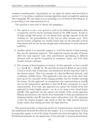
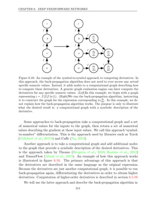
![CHAPTER 6. DEEP FEEDFORWARD NETWORKS
mappings from x to y that lack feedback connections. Other models presented
later will apply these principles to learning stochastic mappings, learning functions
with feedback, and learning probability distributions over a single vector.
We begin this chapter with a simple example of a feedforward network. Next,
we address each of the design decisions needed to deploy a feedforward network.
First, training a feedforward network requires making many of the same design
decisions as are necessary for a linear model: choosing the optimizer, the cost
function, and the form of the output units. We review these basics of gradient-based
learning, then proceed to confront some of the design decisions that are unique
to feedforward networks. Feedforward networks have introduced the concept of a
hidden layer, and this requires us to choose the activation functions that will
be used to compute the hidden layer values. We must also design the architecture
of the network, including how many layers the network should contain, how these
layers should be connected to each other, and how many units should be in
each layer. Learning in deep neural networks requires computing the gradients
of complicated functions. We present the back-propagation algorithm and its
modern generalizations, which can be used to efficiently compute these gradients.
Finally, we close with some historical perspective.
6.1 Example: Learning XOR
To make the idea of a feedforward network more concrete, we begin with an
example of a fully functioning feedforward network on a very simple task: learning
the XOR function.
The XOR function (“exclusive or”) is an operation on two binary values, x1
and x2. When exactly one of these binary values is equal to , the XOR function
1
returns . Otherwise, it returns 0. The XOR function provides the target function
1
y = f∗
(x) that we want to learn. Our model provides a function y = f(x;θ) and
our learning algorithm will adapt the parameters θ to make f as similar as possible
to f∗
.
In this simple example, we will not be concerned with statistical generalization.
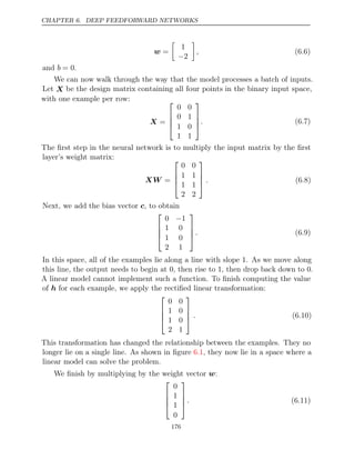
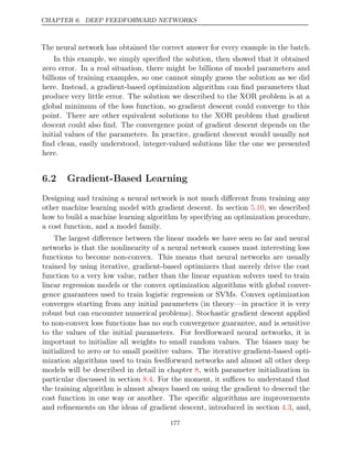
We want our network to perform correctly on the four points X = {[0, 0], [0,1],
[1,0], and [1,1]}. We will train the network on all four of these points. The
only challenge is to fit the training set.
We can treat this problem as a regression problem and use a mean squared
error loss function. We choose this loss function to simplify the math for this
example as much as possible. In practical applications, MSE is usually not an
171](https://image.slidesharecdn.com/deeplearningadaptivecomputationandmachinelearningpdfdrive-230402121325-7c74bca2/85/Deep-learning_-adaptive-computation-and-machine-learning-PDFDrive-pdf-187-320.jpg)
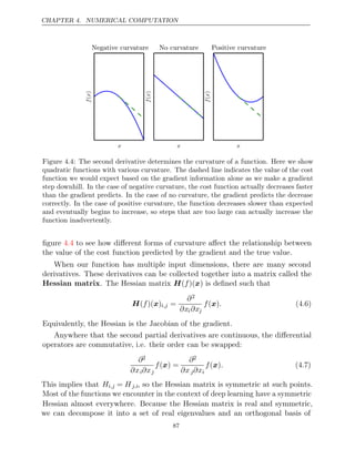
![CHAPTER 6. DEEP FEEDFORWARD NETWORKS
0 1
x1
0
1
x
2
Original space
x
0 1 2
h1
0
1
h
2
Learned space
h
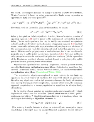
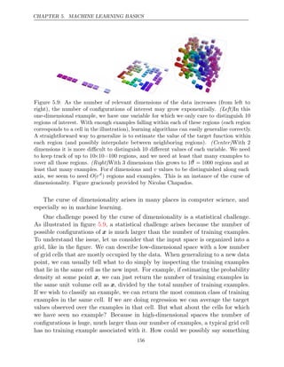
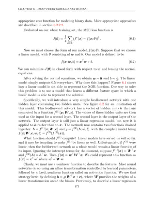
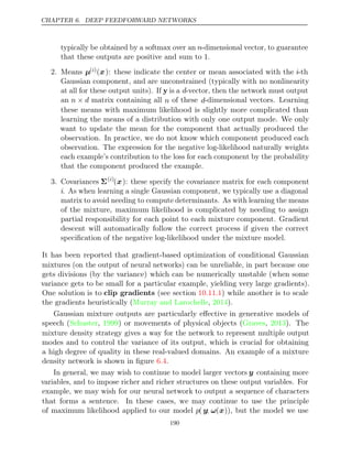
Figure 6.1: Solving the XOR problem by learning a representation. The bold numbers
printed on the plot indicate the value that the learned function must output at each point.
(Left)A linear model applied directly to the original input cannot implement the XOR
function. When x1 = 0, the model’s output must increase as x2 increases. When x1 = 1,
the model’s output must decrease as x2 increases. A linear model must apply a fixed
coefficient w2 to x2. The linear model therefore cannot use the value of x1 to change
the coefficient on x2 and cannot solve this problem. (Right)In the transformed space
represented by the features extracted by a neural network, a linear model can now solve
the problem. In our example solution, the two points that must have output have been
1
collapsed into a single point in feature space. In other words, the nonlinear features have
mapped both x = [1, 0]
and x = [0,1]
to a single point in feature space, h = [1 ,0]
.
The linear model can now describe the function as increasing in h1 and decreasing in h2.
In this example, the motivation for learning the feature space is only to make the model
capacity greater so that it can fit the training set. In more realistic applications, learned
representations can also help the model to generalize.
173](https://image.slidesharecdn.com/deeplearningadaptivecomputationandmachinelearningpdfdrive-230402121325-7c74bca2/85/Deep-learning_-adaptive-computation-and-machine-learning-PDFDrive-pdf-189-320.jpg)
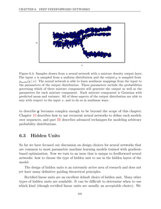
![CHAPTER 6. DEEP FEEDFORWARD NETWORKS
can control the density of the output distribution (for example, by learning the
variance parameter of a Gaussian output distribution) then it becomes possible
to assign extremely high density to the correct training set outputs, resulting in
cross-entropy approaching negative infinity. Regularization techniques described
in chapter provide several different ways of modifying the learning problem so
7
that the model cannot reap unlimited reward in this way.
6.2.1.2 Learning Conditional Statistics
Instead of learning a full probability distribution p(y x
| ; θ) we often want to learn
just one conditional statistic of given .
y x
For example, we may have a predictor f(x;θ) that we wish to predict the mean
of .
y
If we use a sufficiently powerful neural network, we can think of the neural
network as being able to represent any function f from a wide class of functions,
with this class being limited only by features such as continuity and boundedness
rather than by having a specific parametric form. From this point of view, we
can view the cost function as being a functional rather than just a function. A
functional is a mapping from functions to real numbers. We can thus think of
learning as choosing a function rather than merely choosing a set of parameters.
We can design our cost functional to have its minimum occur at some specific
function we desire. For example, we can design the cost functional to have its
minimum lie on the function that maps x to the expected value of y given x.
Solving an optimization problem with respect to a function requires a mathematical
tool called calculus of variations, described in section . It is not necessary
19.4.2
to understand calculus of variations to understand the content of this chapter. At
the moment, it is only necessary to understand that calculus of variations may be
used to derive the following two results.
Our first result derived using calculus of variations is that solving the optimiza-
tion problem
f∗
= arg min
f
Ex y
, ∼pdata || − ||
y f( )
x 2
(6.14)
yields
f∗
( ) =
x Ey∼pdata( )
y x
| [ ]
y , (6.15)
so long as this function lies within the class we optimize over. In other words, if we
could train on infinitely many samples from the true data generating distribution,
minimizing the mean squared error cost function gives a function that predicts the
mean of for each value of .
y x
180](https://image.slidesharecdn.com/deeplearningadaptivecomputationandmachinelearningpdfdrive-230402121325-7c74bca2/85/Deep-learning_-adaptive-computation-and-machine-learning-PDFDrive-pdf-196-320.jpg)
![CHAPTER 6. DEEP FEEDFORWARD NETWORKS
Maximizing the log-likelihood is then equivalent to minimizing the mean squared
error.
The maximum likelihood framework makes it straightforward to learn the
covariance of the Gaussian too, or to make the covariance of the Gaussian be a
function of the input. However, the covariance must be constrained to be a positive
definite matrix for all inputs. It is difficult to satisfy such constraints with a linear
output layer, so typically other output units are used to parametrize the covariance.
Approaches to modeling the covariance are described shortly, in section .
6.2.2.4
Because linear units do not saturate, they pose little difficulty for gradient-
based optimization algorithms and may be used with a wide variety of optimization
algorithms.
6.2.2.2 Sigmoid Units for Bernoulli Output Distributions
Many tasks require predicting the value of a binary variable y. Classification
problems with two classes can be cast in this form.
The maximum-likelihood approach is to define a Bernoulli distribution over y
conditioned on .
x
A Bernoulli distribution is defined by just a single number. The neural net
needs to predict only P(y = 1 | x). For this number to be a valid probability, it
must lie in the interval [0, 1].
Satisfying this constraint requires some careful design effort. Suppose we were
to use a linear unit, and threshold its value to obtain a valid probability:
P y
( = 1 ) = max
| x
0 min
,
1, w
h + b
. (6.18)
This would indeed define a valid conditional distribution, but we would not be able
to train it very effectively with gradient descent. Any time that wh +b strayed
outside the unit interval, the gradient of the output of the model with respect to
its parameters would be 0. A gradient of 0 is typically problematic because the
learning algorithm no longer has a guide for how to improve the corresponding
parameters.
Instead, it is better to use a different approach that ensures there is always a
strong gradient whenever the model has the wrong answer. This approach is based
on using sigmoid output units combined with maximum likelihood.
A sigmoid output unit is defined by
ŷ σ
=
w
h + b
(6.19)
182](https://image.slidesharecdn.com/deeplearningadaptivecomputationandmachinelearningpdfdrive-230402121325-7c74bca2/85/Deep-learning_-adaptive-computation-and-machine-learning-PDFDrive-pdf-198-320.jpg)
![CHAPTER 6. DEEP FEEDFORWARD NETWORKS
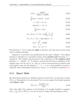
(1 −2y)z, may be simplified to | |
z . As | |
z becomes large while z has the wrong sign,
the softplus function asymptotes toward simply returning its argument | |
z . The
derivative with respect to z asymptotes to sign(z), so, in the limit of extremely
incorrect z, the softplus function does not shrink the gradient at all. This property
is very useful because it means that gradient-based learning can act to quickly
correct a mistaken .
z
When we use other loss functions, such as mean squared error, the loss can
saturate anytime σ(z) saturates. The sigmoid activation function saturates to 0
when z becomes very negative and saturates to when
1 z becomes very positive.
The gradient can shrink too small to be useful for learning whenever this happens,
whether the model has the correct answer or the incorrect answer. For this reason,
maximum likelihood is almost always the preferred approach to training sigmoid
output units.
Analytically, the logarithm of the sigmoid is always defined and finite, because
the sigmoid returns values restricted to the open interval (0, 1), rather than using
the entire closed interval of valid probabilities [0,1]. In software implementations,
to avoid numerical problems, it is best to write the negative log-likelihood as a
function of z, rather than as a function of ŷ = σ(z ). If the sigmoid function
underflows to zero, then taking the logarithm of ŷ yields negative infinity.
6.2.2.3 Softmax Units for Multinoulli Output Distributions
Any time we wish to represent a probability distribution over a discrete variable
with n possible values, we may use the softmax function. This can be seen as a
generalization of the sigmoid function which was used to represent a probability
distribution over a binary variable.
Softmax functions are most often used as the output of a classifier, to represent
the probability distribution over n different classes. More rarely, softmax functions
can be used inside the model itself, if we wish the model to choose between one of
n different options for some internal variable.
In the case of binary variables, we wished to produce a single number
ŷ P y .
= ( = 1 )
| x (6.27)
Because this number needed to lie between and , and because we wanted the
0 1
logarithm of the number to be well-behaved for gradient-based optimization of
the log-likelihood, we chose to instead predict a number z = log P̃(y = 1 | x).
Exponentiating and normalizing gave us a Bernoulli distribution controlled by the
sigmoid function.
184](https://image.slidesharecdn.com/deeplearningadaptivecomputationandmachinelearningpdfdrive-230402121325-7c74bca2/85/Deep-learning_-adaptive-computation-and-machine-learning-PDFDrive-pdf-200-320.jpg)

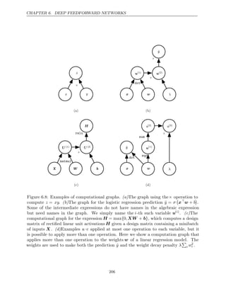
![CHAPTER 6. DEEP FEEDFORWARD NETWORKS
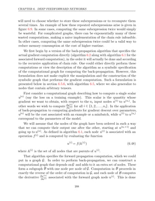
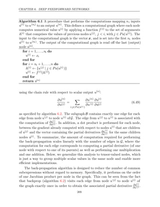
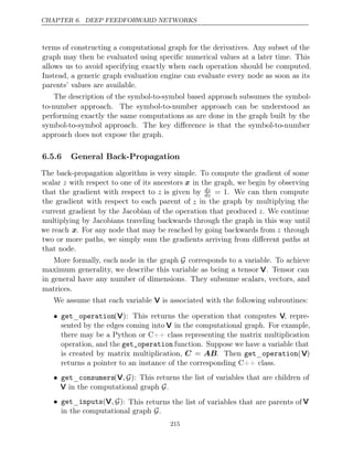
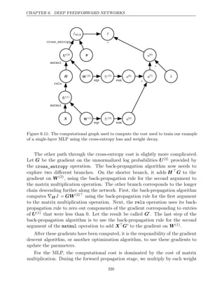
Algorithm 6.2 Simplified version of the back-propagation algorithm for computing
the derivatives of u( )
n
with respect to the variables in the graph. This example is
intended to further understanding by showing a simplified case where all variables
are scalars, and we wish to compute the derivatives with respect to u(1), . . . , u(ni ).
This simplified version computes the derivatives of all nodes in the graph. The
computational cost of this algorithm is proportional to the number of edges in
the graph, assuming that the partial derivative associated with each edge requires
a constant time. This is of the same order as the number of computations for
the forward propagation. Each ∂u( )
i
∂u( )
j is a function of the parents u( )
j
of u( )
i
, thus
linking the nodes of the forward graph to those added for the back-propagation
graph.
Run forward propagation (algorithm for this example) to obtain the activa-
6.1
tions of the network
Initialize grad_table, a data structure that will store the derivatives that have
been computed. The entry grad table
_ [u( )
i
] will store the computed value of
∂u( )
n
∂u( )
i .
grad table
_ [u( )
n ] 1
←
for do
j n
= − 1 down to 1
The next line computes ∂u( )
n
∂u( )
j =
i j P a u
: ∈ ( ( )
i )
∂u( )
n
∂u( )
i
∂u ( )
i
∂u( )
j using stored values:
grad table
_ [u( )
j ] ←
i j P a u
: ∈ ( ( )
i ) grad table
_ [u( )
i ]∂u( )
i
∂u( )
j
end for
return {grad table
_ [u( )
i ] = 1
| i , . . . , ni}
Back-propagation thus avoids the exponential explosion in repeated subexpressions.
However, other algorithms may be able to avoid more subexpressions by performing
simplifications on the computational graph, or may be able to conserve memory by
recomputing rather than storing some subexpressions. We will revisit these ideas
after describing the back-propagation algorithm itself.
6.5.4 Back-Propagation Computation in Fully-Connected MLP
To clarify the above definition of the back-propagation computation, let us consider
the specific graph associated with a fully-connected multi-layer MLP.
Algorithm first shows the forward propagation, which maps parameters to
6.3
the supervised loss L(ŷ y
, ) associated with a single (input,target) training example
( )
x y
, , with ŷ the output of the neural network when is provided in input.
x
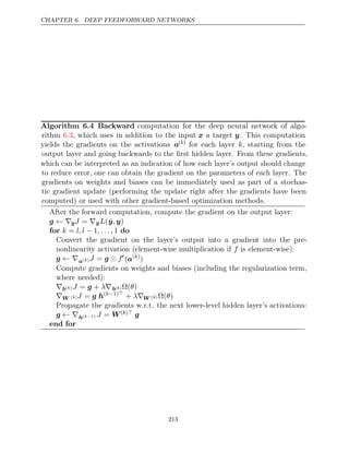
Algorithm then shows the corresponding computation to be done for
6.4
210](https://image.slidesharecdn.com/deeplearningadaptivecomputationandmachinelearningpdfdrive-230402121325-7c74bca2/85/Deep-learning_-adaptive-computation-and-machine-learning-PDFDrive-pdf-226-320.jpg)
![CHAPTER 6. DEEP FEEDFORWARD NETWORKS
applying the back-propagation algorithm to this graph.
Algorithms and are demonstrations that are chosen to be simple and
6.3 6.4
straightforward to understand. However, they are specialized to one specific
problem.
Modern software implementations are based on the generalized form of back-
propagation described in section below, which can accommodate any compu-
6.5.6
tational graph by explicitly manipulating a data structure for representing symbolic
computation.
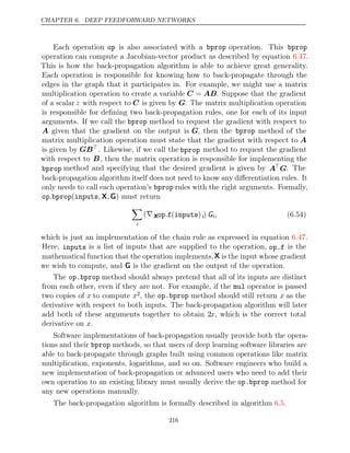
Algorithm 6.3 Forward propagation through a typical deep neural network and
the computation of the cost function. The loss L(ŷ y
, ) depends on the output
ŷ and on the target y (see section for examples of loss functions). To
6.2.1.1
obtain the total cost J, the loss may be added to a regularizer Ω(θ), where θ
contains all the parameters (weights and biases). Algorithm shows how to
6.4
compute gradients of J with respect to parameters W and b. For simplicity, this
demonstration uses only a single input example x. Practical applications should
use a minibatch. See section for a more realistic demonstration.
6.5.7
Require: Network depth, l
Require: W ( )
i , i , . . . , l ,
∈ {1 } the weight matrices of the model
Require: b( )
i , i , . . . , l ,
∈ {1 } the bias parameters of the model
Require: x, the input to process
Require: y, the target output
h(0) = x
for do
k , . . . , l
= 1
a( )
k = b( )
k + W( )
k h( 1)
k−
h( )
k
= (
f a( )
k
)
end for
ŷ h
= ( )
l
J L
= (ŷ y
, ) + Ω( )
λ θ
6.5.5 Symbol-to-Symbol Derivatives
Algebraic expressions and computational graphs both operate on symbols, or
variables that do not have specific values. These algebraic and graph-based
representations are called symbolic representations. When we actually use or
train a neural network, we must assign specific values to these symbols. We
replace a symbolic input to the network x with a specific numeric value, such as
[1 2 3 765 1 8]
. , . , − .
.
212](https://image.slidesharecdn.com/deeplearningadaptivecomputationandmachinelearningpdfdrive-230402121325-7c74bca2/85/Deep-learning_-adaptive-computation-and-machine-learning-PDFDrive-pdf-228-320.jpg)
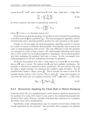
![CHAPTER 6. DEEP FEEDFORWARD NETWORKS
Algorithm 6.5 The outermost skeleton of the back-propagation algorithm. This
portion does simple setup and cleanup work. Most of the important work happens
in the subroutine of algorithm
build_grad 6.6
.
Require: T, the target set of variables whose gradients must be computed.
Require: G, the computational graph
Require: z, the variable to be differentiated
Let G
be G pruned to contain only nodes that are ancestors of z and descendents
of nodes in .
T
Initialize , a data structure associating tensors to their gradients
grad_table
grad table
_ [ ] 1
z ←
for do
V in T
build grad
_ (V, ,
G G , grad table
_ )
end for
Return restricted to
grad_table T
In section , we explained that back-propagation was developed in order to
6.5.2
avoid computing the same subexpression in the chain rule multiple times. The naive
algorithm could have exponential runtime due to these repeated subexpressions.
Now that we have specified the back-propagation algorithm, we can understand its
computational cost. If we assume that each operation evaluation has roughly the
same cost, then we may analyze the computational cost in terms of the number
of operations executed. Keep in mind here that we refer to an operation as the
fundamental unit of our computational graph, which might actually consist of very
many arithmetic operations (for example, we might have a graph that treats matrix
multiplication as a single operation). Computing a gradient in a graph with n nodes
will never execute more than O(n2) operations or store the output of more than
O(n2) operations. Here we are counting operations in the computational graph, not
individual operations executed by the underlying hardware, so it is important to
remember that the runtime of each operation may be highly variable. For example,
multiplying two matrices that each contain millions of entries might correspond to
a single operation in the graph. We can see that computing the gradient requires as
most O(n2
) operations because the forward propagation stage will at worst execute
all n nodes in the original graph (depending on which values we want to compute,
we may not need to execute the entire graph). The back-propagation algorithm
adds one Jacobian-vector product, which should be expressed with O(1) nodes, per
edge in the original graph. Because the computational graph is a directed acyclic
graph it has at most O(n2 ) edges. For the kinds of graphs that are commonly used
in practice, the situation is even better. Most neural network cost functions are
217](https://image.slidesharecdn.com/deeplearningadaptivecomputationandmachinelearningpdfdrive-230402121325-7c74bca2/85/Deep-learning_-adaptive-computation-and-machine-learning-PDFDrive-pdf-233-320.jpg)
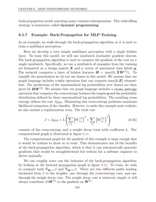
![CHAPTER 6. DEEP FEEDFORWARD NETWORKS
Algorithm 6.6 The inner loop subroutine build grad
_ (V, ,
G G, grad table
_ ) of
the back-propagation algorithm, called by the back-propagation algorithm defined
in algorithm .
6.5
Require: V, the variable whose gradient should be added to and .
G grad_table
Require: G, the graph to modify.
Require: G
, the restriction of to nodes that participate in the gradient.
G
Require: grad_table, a data structure mapping nodes to their gradients
if then
V is in grad_table
Return _
grad table[ ]
V
end if
i ← 1
for C V
in _
get consumers( , G) do
op get operation
← _ ( )
C
D C
← build grad
_ ( , ,
G G, grad table
_ )
G( )
i
← G
op bprop get inputs
. ( _ (C, ) )
, ,
V D
i i
← + 1
end for
G ←
i G( )
i
grad table
_ [ ] =
V G
Insert and the operations creating it into
G G
Return G
roughly chain-structured, causing back-propagation to have O(n) cost. This is far
better than the naive approach, which might need to execute exponentially many
nodes. This potentially exponential cost can be seen by expanding and rewriting
the recursive chain rule (equation ) non-recursively:
6.49
∂u( )
n
∂u( )
j
=
path (u(π1),u(π
2),...,u(πt)),
from π1= to
j πt=n
t
k=2
∂u(πk)
∂u(πk−1 )
. (6.55)
Since the number of paths from node j to node n can grow exponentially in the
length of these paths, the number of terms in the above sum, which is the number
of such paths, can grow exponentially with the depth of the forward propagation
graph. This large cost would be incurred because the same computation for
∂u( )
i
∂u( )
j would be redone many times. To avoid such recomputation, we can think
of back-propagation as a table-filling algorithm that takes advantage of storing
intermediate results ∂u( )
n
∂u( )
i . Each node in the graph has a corresponding slot in a
table to store the gradient for that node. By filling in these table entries in order,
218](https://image.slidesharecdn.com/deeplearningadaptivecomputationandmachinelearningpdfdrive-230402121325-7c74bca2/85/Deep-learning_-adaptive-computation-and-machine-learning-PDFDrive-pdf-234-320.jpg)
![CHAPTER 7. REGULARIZATION FOR DEEP LEARNING
of regularization. As with L2
weight decay, L1
weight decay controls the strength
of the regularization by scaling the penalty using a positive hyperparameter
Ω α.
Thus, the regularized objective function ˜
J ,
( ;
w X y) is given by
J̃ , α
( ;
w X y) = || ||
w 1 + ( ; )
J w X y
, , (7.19)
with the corresponding gradient (actually, sub-gradient):
∇w ˜
J , α
( ;
w X y) = sign( ) +
w ∇wJ ,
(X y w
; ) (7.20)
where is simply the sign of applied element-wise.
sign( )
w w
By inspecting equation , we can see immediately that the effect of
7.20 L1
regularization is quite different from that of L2
regularization. Specifically, we can
see that the regularization contribution to the gradient no longer scales linearly
with each wi; instead it is a constant factor with a sign equal to sign(wi). One
consequence of this form of the gradient is that we will not necessarily see clean
algebraic solutions to quadratic approximations of J(X y
, ;w) as we did for L2
regularization.
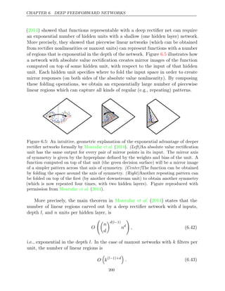
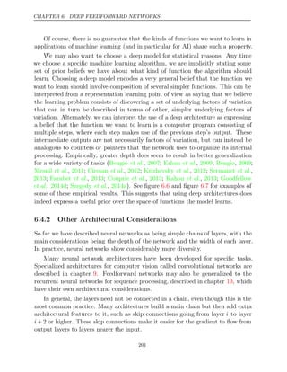
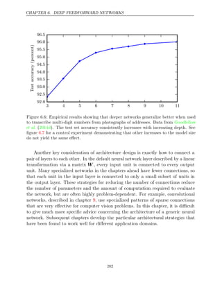
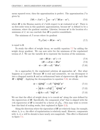
Our simple linear model has a quadratic cost function that we can represent
via its Taylor series. Alternately, we could imagine that this is a truncated Taylor
series approximating the cost function of a more sophisticated model. The gradient
in this setting is given by
∇w ˆ
J( ) = (
w H w w
− ∗
), (7.21)
where, again, is the Hessian matrix of with respect to evaluated at
H J w w∗.
Because the L1
penalty does not admit clean algebraic expressions in the case
of a fully general Hessian, we will also make the further simplifying assumption
that the Hessian is diagonal, H = diag([H1 1
, , . . . , Hn,n ]), where each Hi,i > 0.
This assumption holds if the data for the linear regression problem has been
preprocessed to remove all correlation between the input features, which may be
accomplished using PCA.
Our quadratic approximation of the L1 regularized objective function decom-
poses into a sum over the parameters:
Ĵ , J
( ;
w X y) = (w∗
; ) +
X y
,
i
1
2
Hi,i(wi − w∗
i )2
+ α w
| i|
. (7.22)
The problem of minimizing this approximate cost function has an analytical solution
(for each dimension ), with the following form:
i
wi = sign(w∗
i ) max
|w∗
i | −
α
Hi,i
, 0
. (7.23)
235](https://image.slidesharecdn.com/deeplearningadaptivecomputationandmachinelearningpdfdrive-230402121325-7c74bca2/85/Deep-learning_-adaptive-computation-and-machine-learning-PDFDrive-pdf-251-320.jpg)
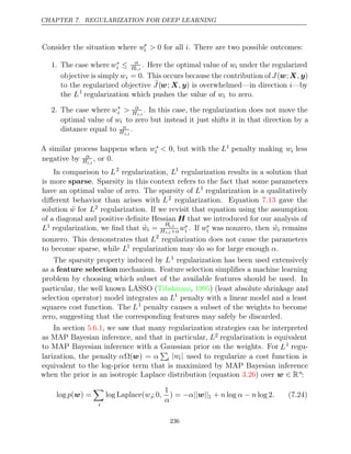
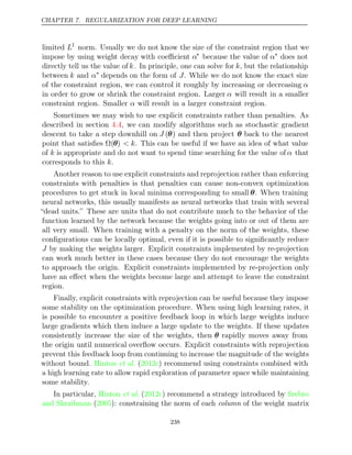
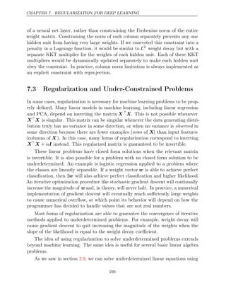
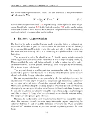
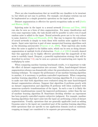
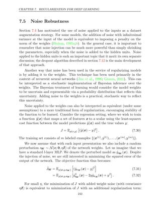
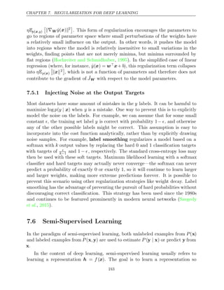
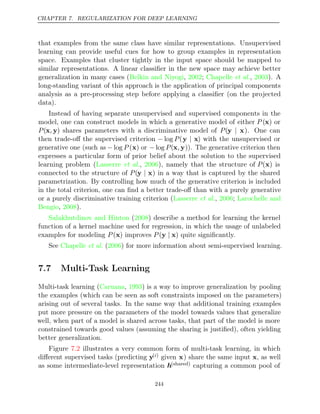
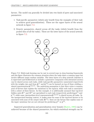
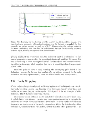
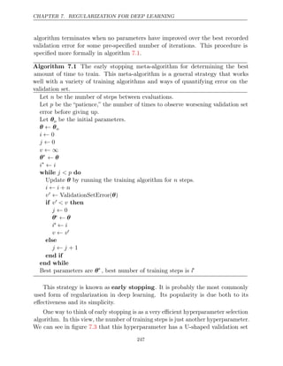
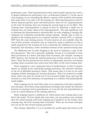
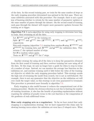
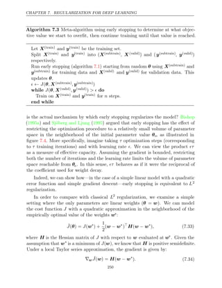
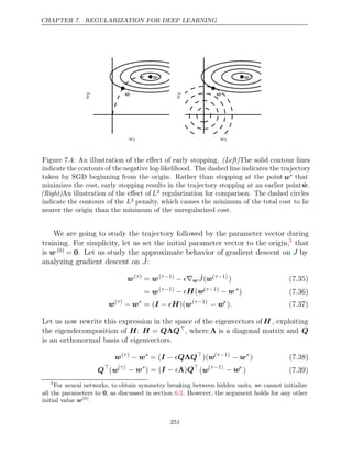
![CHAPTER 7. REGULARIZATION FOR DEEP LEARNING
Assuming that w(0)
= 0 and that is chosen to be small enough to guarantee
|1− λi| < 1, the parameter trajectory during training after τ parameter updates
is as follows:
Q
w( )
τ
= [ ( )
I − I − Λ τ
]Q
w∗
. (7.40)
Now, the expression for Q
w̃ in equation for
7.13 L2
regularization can be rear-
ranged as:
Q
w̃ I
= ( +
Λ α )−1
ΛQ
w∗
(7.41)
Q
w̃ I I
= [ − ( +
Λ α )−1
α]Q
w∗
(7.42)
Comparing equation and equation , we see that if the hyperparameters
7.40 7.42 ,
α τ
, and are chosen such that
( )
I − Λ τ
= ( + )
Λ αI −1
α, (7.43)
then L2 regularization and early stopping can be seen to be equivalent (at least
under the quadratic approximation of the objective function). Going even further,
by taking logarithms and using the series expansion for log(1 +x), we can conclude
that if all λi are small (that is, λi 1 and λi/α 1) then
τ ≈
1
α
, (7.44)
α ≈
1
τ
. (7.45)
That is, under these assumptions, the number of training iterations τ plays a role
inversely proportional to the L2
regularization parameter, and the inverse of τ
plays the role of the weight decay coefficient.
Parameter values corresponding to directions of significant curvature (of the
objective function) are regularized less than directions of less curvature. Of course,
in the context of early stopping, this really means that parameters that correspond
to directions of significant curvature tend to learn early relative to parameters
corresponding to directions of less curvature.
The derivations in this section have shown that a trajectory of length τ ends
at a point that corresponds to a minimum of the L2-regularized objective. Early
stopping is of course more than the mere restriction of the trajectory length;
instead, early stopping typically involves monitoring the validation set error in
order to stop the trajectory at a particularly good point in space. Early stopping
therefore has the advantage over weight decay that early stopping automatically
determines the correct amount of regularization while weight decay requires many
training experiments with different values of its hyperparameter.
252](https://image.slidesharecdn.com/deeplearningadaptivecomputationandmachinelearningpdfdrive-230402121325-7c74bca2/85/Deep-learning_-adaptive-computation-and-machine-learning-PDFDrive-pdf-268-320.jpg)
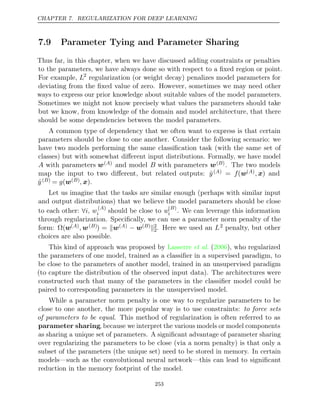
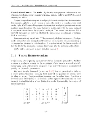
![CHAPTER 7. REGULARIZATION FOR DEEP LEARNING
OMP-k with the value of k specified to indicate the number of non-zero features
allowed. ( ) demonstrated that OMP- can be a very effective
Coates and Ng 2011 1
feature extractor for deep architectures.
Essentially any model that has hidden units can be made sparse. Throughout
this book, we will see many examples of sparsity regularization used in a variety of
contexts.
7.11 Bagging and Other Ensemble Methods
Bagging (short for bootstrap aggregating) is a technique for reducing gen-
eralization error by combining several models ( , ). The idea is to
Breiman 1994
train several different models separately, then have all of the models vote on the
output for test examples. This is an example of a general strategy in machine
learning called model averaging. Techniques employing this strategy are known
as ensemble methods.
The reason that model averaging works is that different models will usually
not make all the same errors on the test set.
Consider for example a set of k regression models. Suppose that each model
makes an error i on each example, with the errors drawn from a zero-mean
multivariate normal distribution with variances E[2
i] = v and covariances E[ij] =
c. Then the error made by the average prediction of all the ensemble models is
1
k
i i. The expected squared error of the ensemble predictor is
E
1
k
i
i
2
=
1
k2 E
i
2
i +
j i
=
ij
(7.50)
=
1
k
v +
k − 1
k
c. (7.51)
In the case where the errors are perfectly correlated and c = v, the mean squared
error reduces to v, so the model averaging does not help at all. In the case where
the errors are perfectly uncorrelated and c = 0, the expected squared error of the
ensemble is only 1
k v. This means that the expected squared error of the ensemble
decreases linearly with the ensemble size. In other words, on average, the ensemble
will perform at least as well as any of its members, and if the members make
independent errors, the ensemble will perform significantly better than its members.
Different ensemble methods construct the ensemble of models in different ways.
For example, each member of the ensemble could be formed by training a completely
256](https://image.slidesharecdn.com/deeplearningadaptivecomputationandmachinelearningpdfdrive-230402121325-7c74bca2/85/Deep-learning_-adaptive-computation-and-machine-learning-PDFDrive-pdf-272-320.jpg)
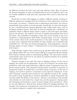
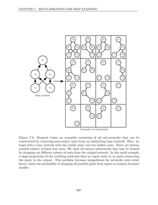
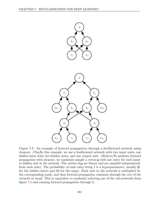
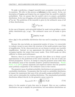
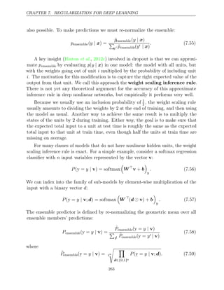
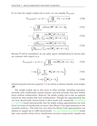
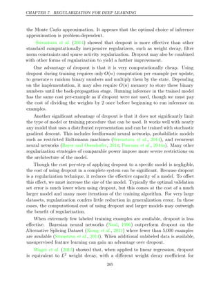
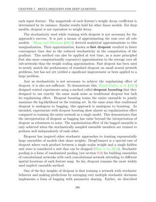
![CHAPTER 7. REGULARIZATION FOR DEEP LEARNING
dropout as bagging an ensemble of models formed by including or excluding
units. However, there is no need for this model averaging strategy to be based on
inclusion and exclusion. In principle, any kind of random modification is admissible.
In practice, we must choose modification families that neural networks are able
to learn to resist. Ideally, we should also use model families that allow a fast
approximate inference rule. We can think of any form of modification parametrized
by a vector µ as training an ensemble consisting of p(y ,
| x µ) for all possible
values of µ. There is no requirement that µ have a finite number of values. For
example, µ can be real-valued. Srivastava 2014
et al. ( ) showed that multiplying the
weights by µ ∼ N (1, I) can outperform dropout based on binary masks. Because
E[µ] = 1 the standard network automatically implements approximate inference
in the ensemble, without needing any weight scaling.
So far we have described dropout purely as a means of performing efficient,
approximate bagging. However, there is another view of dropout that goes further
than this. Dropout trains not just a bagged ensemble of models, but an ensemble
of models that share hidden units. This means each hidden unit must be able to
perform well regardless of which other hidden units are in the model. Hidden units
must be prepared to be swapped and interchanged between models. Hinton et al.
( ) were inspired by an idea from biology: sexual reproduction, which involves
2012c
swapping genes between two different organisms, creates evolutionary pressure for
genes to become not just good, but to become readily swapped between different
organisms. Such genes and such features are very robust to changes in their
environment because they are not able to incorrectly adapt to unusual features
of any one organism or model. Dropout thus regularizes each hidden unit to be
not merely a good feature but a feature that is good in many contexts. Warde-
Farley 2014
et al. ( ) compared dropout training to training of large ensembles and
concluded that dropout offers additional improvements to generalization error
beyond those obtained by ensembles of independent models.
It is important to understand that a large portion of the power of dropout
arises from the fact that the masking noise is applied to the hidden units. This
can be seen as a form of highly intelligent, adaptive destruction of the information
content of the input rather than destruction of the raw values of the input. For
example, if the model learns a hidden unit hi that detects a face by finding the nose,
then dropping hi corresponds to erasing the information that there is a nose in
the image. The model must learn another hi, either that redundantly encodes the
presence of a nose, or that detects the face by another feature, such as the mouth.
Traditional noise injection techniques that add unstructured noise at the input are
not able to randomly erase the information about a nose from an image of a face
unless the magnitude of the noise is so great that nearly all of the information in
267](https://image.slidesharecdn.com/deeplearningadaptivecomputationandmachinelearningpdfdrive-230402121325-7c74bca2/85/Deep-learning_-adaptive-computation-and-machine-learning-PDFDrive-pdf-283-320.jpg)
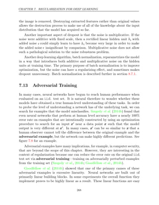
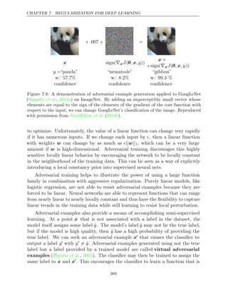
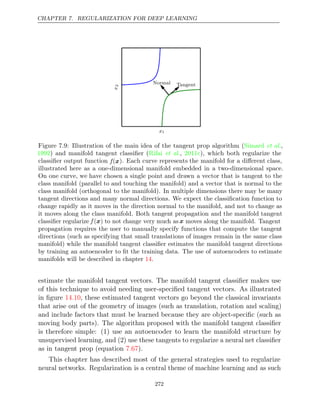

![CHAPTER 8. OPTIMIZATION FOR TRAINING DEEP MODELS
solvable by an optimization algorithm. However, when we do not know pdata(x, y)
but only have a training set of samples, we have a machine learning problem.
The simplest way to convert a machine learning problem back into an op-
timization problem is to minimize the expected loss on the training set. This
means replacing the true distribution p(x, y) with the empirical distribution p̂(x, y)
defined by the training set. We now minimize the empirical risk
Ex,y∼p̂data( )
x,y [ ( ( ; ) )] =
L f x θ , y
1
m
m
i=1
L f
( (x( )
i
; )
θ , y( )
i
) (8.3)
where is the number of training examples.
m
The training process based on minimizing this average training error is known
as empirical risk minimization. In this setting, machine learning is still very
similar to straightforward optimization. Rather than optimizing the risk directly,
we optimize the empirical risk, and hope that the risk decreases significantly as
well. A variety of theoretical results establish conditions under which the true risk
can be expected to decrease by various amounts.
However, empirical risk minimization is prone to overfitting. Models with
high capacity can simply memorize the training set. In many cases, empirical
risk minimization is not really feasible. The most effective modern optimization
algorithms are based on gradient descent, but many useful loss functions, such
as 0-1 loss, have no useful derivatives (the derivative is either zero or undefined
everywhere). These two problems mean that, in the context of deep learning, we
rarely use empirical risk minimization. Instead, we must use a slightly different
approach, in which the quantity that we actually optimize is even more different
from the quantity that we truly want to optimize.
8.1.2 Surrogate Loss Functions and Early Stopping
Sometimes, the loss function we actually care about (say classification error) is not
one that can be optimized efficiently. For example, exactly minimizing expected 0-1
loss is typically intractable (exponential in the input dimension), even for a linear
classifier (Marcotte and Savard 1992
, ). In such situations, one typically optimizes
a surrogate loss function instead, which acts as a proxy but has advantages.
For example, the negative log-likelihood of the correct class is typically used as a
surrogate for the 0-1 loss. The negative log-likelihood allows the model to estimate
the conditional probability of the classes, given the input, and if the model can
do that well, then it can pick the classes that yield the least classification error in
expectation.
276](https://image.slidesharecdn.com/deeplearningadaptivecomputationandmachinelearningpdfdrive-230402121325-7c74bca2/85/Deep-learning_-adaptive-computation-and-machine-learning-PDFDrive-pdf-292-320.jpg)
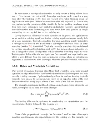
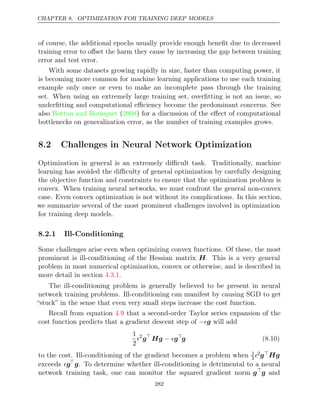
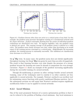
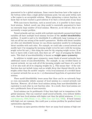
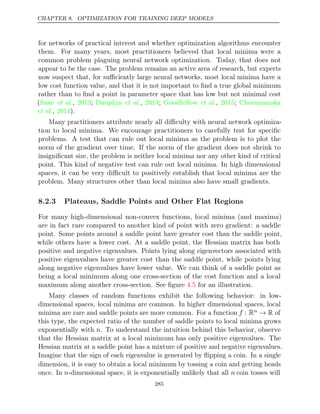
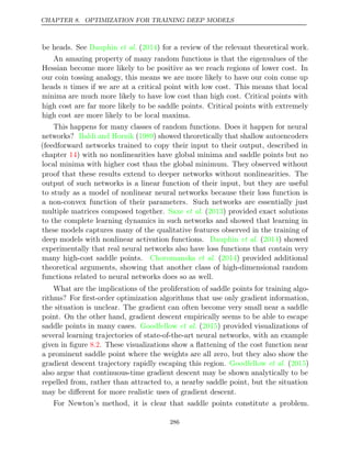
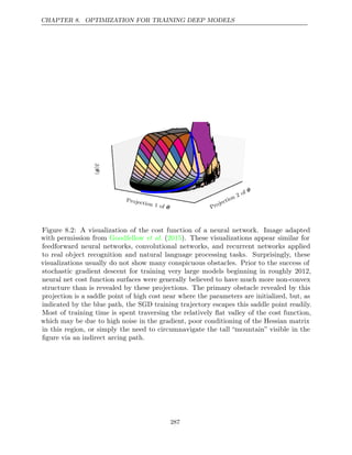
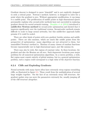
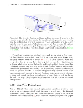
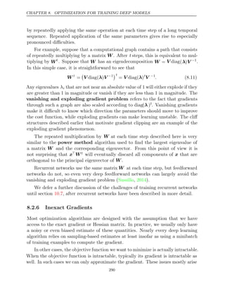
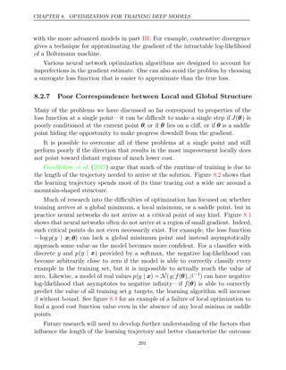
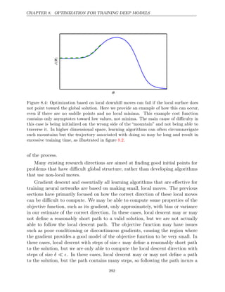
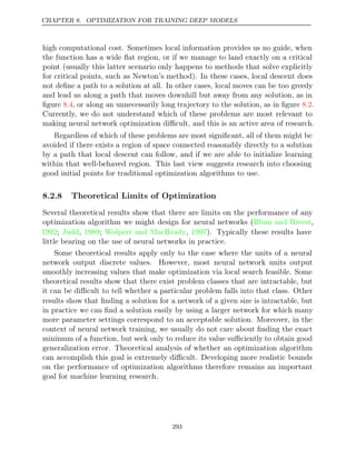
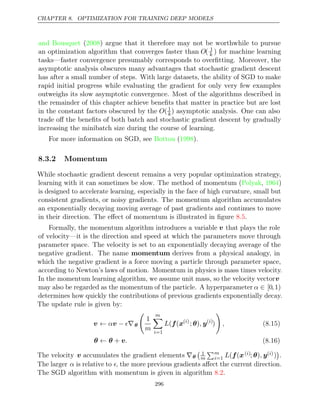
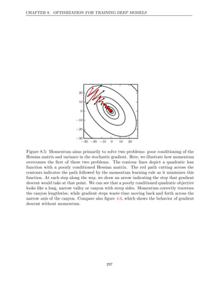
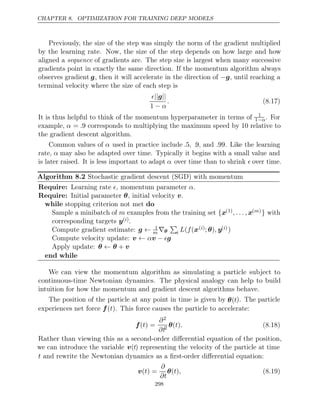
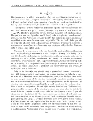
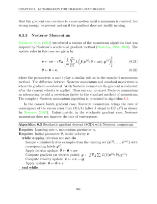
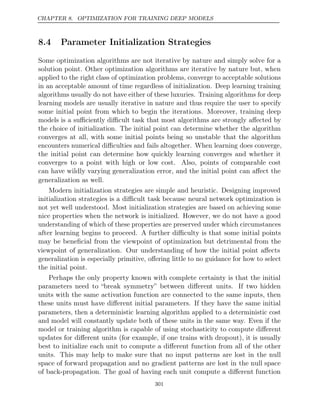
![CHAPTER 8. OPTIMIZATION FOR TRAINING DEEP MODELS
increasing its weights, it is possible to eventually obtain a network with reasonable
initial activations throughout. If learning is still too slow at this point, it can be
useful to look at the range or standard deviation of the gradients as well as the
activations. This procedure can in principle be automated and is generally less
computationally costly than hyperparameter optimization based on validation set
error because it is based on feedback from the behavior of the initial model on a
single batch of data, rather than on feedback from a trained model on the validation
set. While long used heuristically, this protocol has recently been specified more
formally and studied by ( ).
Mishkin and Matas 2015
So far we have focused on the initialization of the weights. Fortunately,
initialization of other parameters is typically easier.
The approach for setting the biases must be coordinated with the approach
for settings the weights. Setting the biases to zero is compatible with most weight
initialization schemes. There are a few situations where we may set some biases to
non-zero values:
• If a bias is for an output unit, then it is often beneficial to initialize the bias to
obtain the right marginal statistics of the output. To do this, we assume that
the initial weights are small enough that the output of the unit is determined
only by the bias. This justifies setting the bias to the inverse of the activation
function applied to the marginal statistics of the output in the training set.
For example, if the output is a distribution over classes and this distribution
is a highly skewed distribution with the marginal probability of class i given
by element ci of some vector c, then we can set the bias vector b by solving
the equation softmax(b) = c. This applies not only to classifiers but also to
models we will encounter in Part , such as autoencoders and Boltzmann
III
machines. These models have layers whose output should resemble the input
data x, and it can be very helpful to initialize the biases of such layers to
match the marginal distribution over .
x
• Sometimes we may want to choose the bias to avoid causing too much
saturation at initialization. For example, we may set the bias of a ReLU
hidden unit to 0.1 rather than 0 to avoid saturating the ReLU at initialization.
This approach is not compatible with weight initialization schemes that do
not expect strong input from the biases though. For example, it is not
recommended for use with random walk initialization ( , ).
Sussillo 2014
• Sometimes a unit controls whether other units are able to participate in a
function. In such situations, we have a unit with output u and another unit
h ∈ [0, 1], and they are multiplied together to produce an output uh. We
305](https://image.slidesharecdn.com/deeplearningadaptivecomputationandmachinelearningpdfdrive-230402121325-7c74bca2/85/Deep-learning_-adaptive-computation-and-machine-learning-PDFDrive-pdf-321-320.jpg)
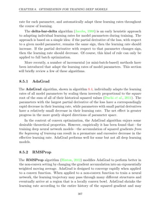
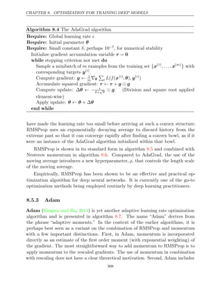
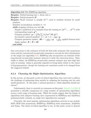
![CHAPTER 8. OPTIMIZATION FOR TRAINING DEEP MODELS
Algorithm 8.6 RMSProp algorithm with Nesterov momentum
Require: Global learning rate , decay rate , momentum coefficient .
ρ α
Require: Initial parameter , initial velocity .
θ v
Initialize accumulation variable r = 0
while do
stopping criterion not met
Sample a minibatch of m examples from the training set {x(1)
, . . . , x( )
m } with
corresponding targets y( )
i
.
Compute interim update: θ̃ θ v
← + α
Compute gradient: g ← 1
m∇θ̃
i L f
( (x( )
i
; ˜
θ y
), ( )
i
)
Accumulate gradient: r r g g
← ρ + (1 )
− ρ
Compute velocity update: v v
← α −
√
r g. ( 1
√
r applied element-wise)
Apply update: θ θ v
← +
end while
largely on the user’s familiarity with the algorithm (for ease of hyperparameter
tuning).
8.6 Approximate Second-Order Methods
In this section we discuss the application of second-order methods to the training
of deep networks. See ( ) for an earlier treatment of this subject.
LeCun et al. 1998a
For simplicity of exposition, the only objective function we examine is the empirical
risk:
J( ) =
θ Ex,y∼p̂data ( )
x,y [ ( ( ; ) )] =
L f x θ , y
1
m
m
i=1
L f
( (x( )
i
; )
θ , y( )
i
). (8.25)
However the methods we discuss here extend readily to more general objective
functions that, for instance, include parameter regularization terms such as those
discussed in chapter .
7
8.6.1 Newton’s Method
In section , we introduced second-order gradient methods. In contrast to first-
4.3
order methods, second-order methods make use of second derivatives to improve
optimization. The most widely used second-order method is Newton’s method. We
now describe Newton’s method in more detail, with emphasis on its application to
neural network training.
310](https://image.slidesharecdn.com/deeplearningadaptivecomputationandmachinelearningpdfdrive-230402121325-7c74bca2/85/Deep-learning_-adaptive-computation-and-machine-learning-PDFDrive-pdf-326-320.jpg)
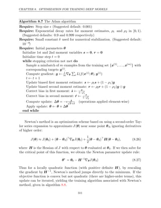
![CHAPTER 8. OPTIMIZATION FOR TRAINING DEEP MODELS
Algorithm 8.8 Newton’s method with objective J(θ) =
1
m
m
i=1 L f
( (x( )
i
; )
θ , y( )
i
).
Require: Initial parameter θ0
Require: Training set of examples
m
while do
stopping criterion not met
Compute gradient: g ← 1
m∇θ
i L f
( (x( )
i
; )
θ , y( )
i
)
Compute Hessian: H ← 1
m ∇2
θ
i L f
( (x( )
i ; )
θ , y( )
i )
Compute Hessian inverse: H−1
Compute update: ∆ =
θ −H−1
g
Apply update: θ θ θ
= + ∆
end while
For surfaces that are not quadratic, as long as the Hessian remains positive
definite, Newton’s method can be applied iteratively. This implies a two-step
iterative procedure. First, update or compute the inverse Hessian (i.e. by updat-
ing the quadratic approximation). Second, update the parameters according to
equation .
8.27
In section , we discussed how Newton’s method is appropriate only when
8.2.3
the Hessian is positive definite. In deep learning, the surface of the objective
function is typically non-convex with many features, such as saddle points, that
are problematic for Newton’s method. If the eigenvalues of the Hessian are not
all positive, for example, near a saddle point, then Newton’s method can actually
cause updates to move in the wrong direction. This situation can be avoided
by regularizing the Hessian. Common regularization strategies include adding a
constant, , along the diagonal of the Hessian. The regularized update becomes
α
θ∗
= θ0 − [ ( (
H f θ0)) + ]
αI −1
∇θ f(θ0). (8.28)
This regularization strategy is used in approximations to Newton’s method, such
as the Levenberg–Marquardt algorithm (Levenberg 1944 Marquardt 1963
, ; , ), and
works fairly well as long as the negative eigenvalues of the Hessian are still relatively
close to zero. In cases where there are more extreme directions of curvature, the
value of α would have to be sufficiently large to offset the negative eigenvalues.
However, as α increases in size, the Hessian becomes dominated by the αI diagonal
and the direction chosen by Newton’s method converges to the standard gradient
divided by α. When strong negative curvature is present, α may need to be so
large that Newton’s method would make smaller steps than gradient descent with
a properly chosen learning rate.
Beyond the challenges created by certain features of the objective function,
312](https://image.slidesharecdn.com/deeplearningadaptivecomputationandmachinelearningpdfdrive-230402121325-7c74bca2/85/Deep-learning_-adaptive-computation-and-machine-learning-PDFDrive-pdf-328-320.jpg)
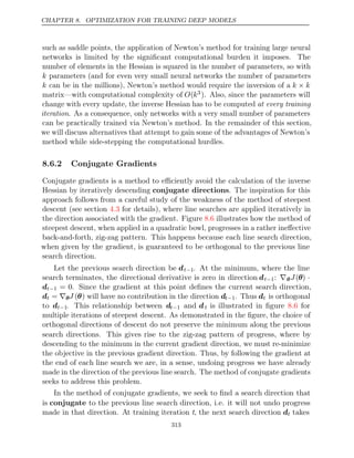
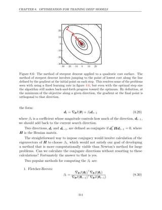
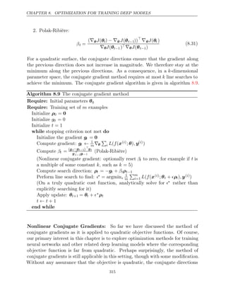
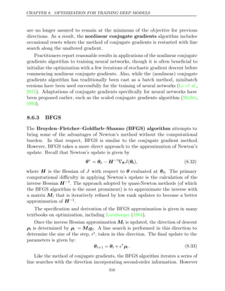
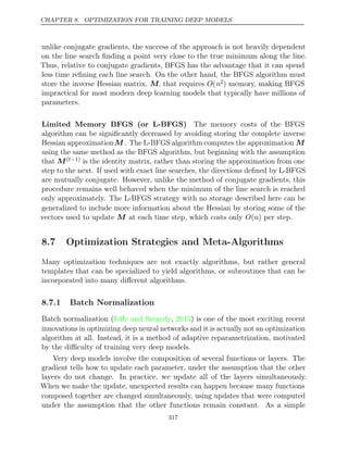
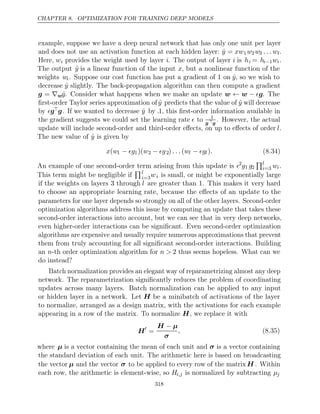
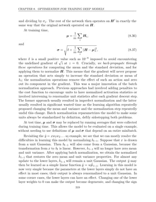
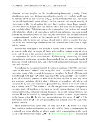
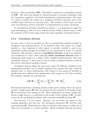
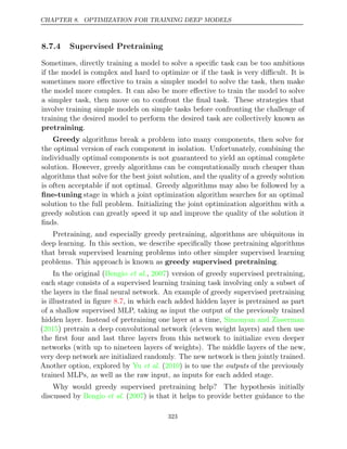
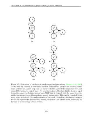
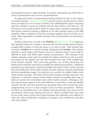
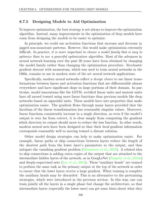
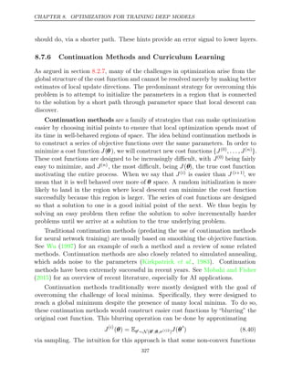
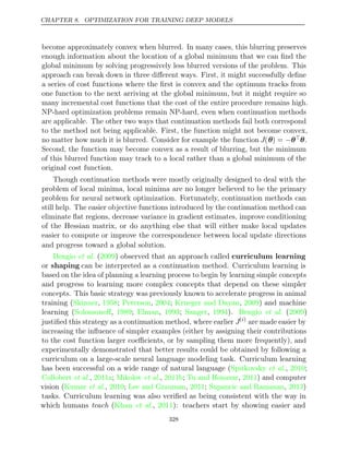
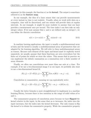
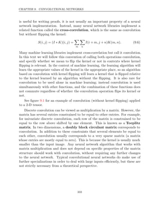

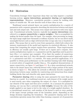
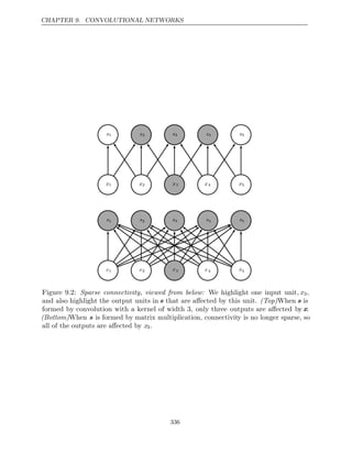
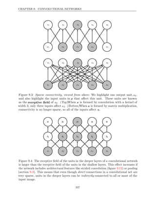
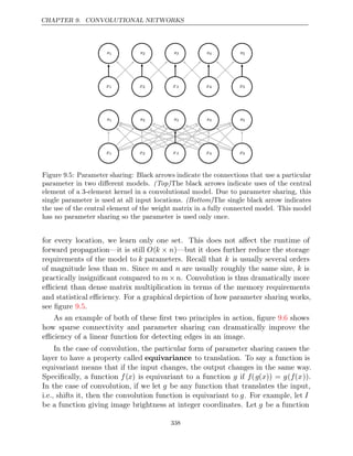
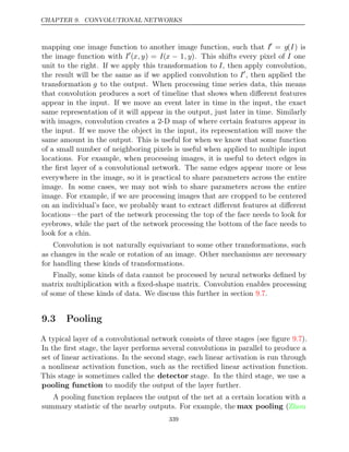
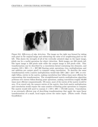
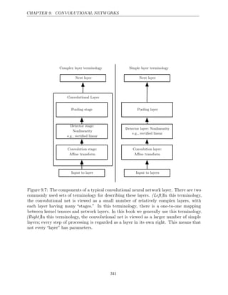
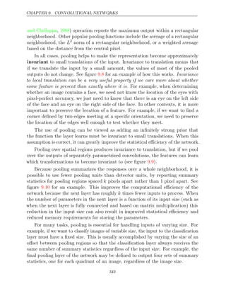
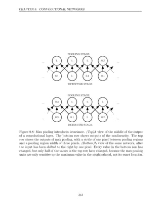
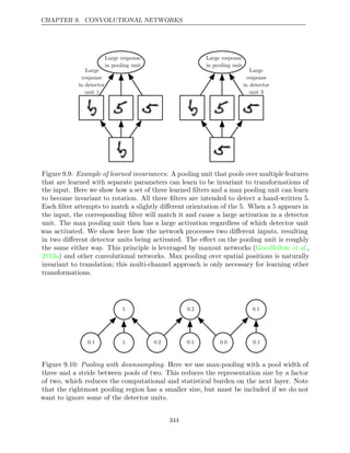
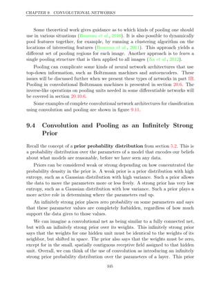
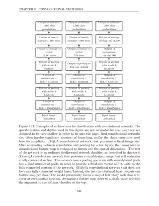
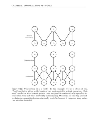
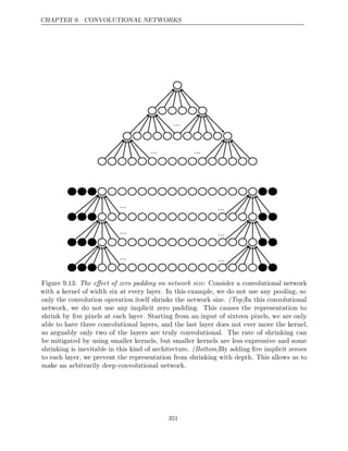
![CHAPTER 9. CONVOLUTIONAL NETWORKS
In some cases, we do not actually want to use convolution, but rather locally
connected layers ( , , ). In this case, the adjacency matrix in the
LeCun 1986 1989
graph of our MLP is the same, but every connection has its own weight, specified
by a 6-D tensor W. The indices into W are respectively: i, the output channel,
j, the output row, k, the output column, l, the input channel, m, the row offset
within the input, and n, the column offset within the input. The linear part of a
locally connected layer is then given by
Zi,j,k =
l,m,n
[Vl,j m ,k n
+ −1 + −1wi,j,k,l,m,n]. (9.9)
This is sometimes also called unshared convolution, because it is a similar oper-
ation to discrete convolution with a small kernel, but without sharing parameters
across locations. Figure compares local connections, convolution, and full
9.14
connections.
Locally connected layers are useful when we know that each feature should be
a function of a small part of space, but there is no reason to think that the same
feature should occur across all of space. For example, if we want to tell if an image
is a picture of a face, we only need to look for the mouth in the bottom half of the
image.
It can also be useful to make versions of convolution or locally connected layers
in which the connectivity is further restricted, for example to constrain each output
channel i to be a function of only a subset of the input channels l. A common
way to do this is to make the first m output channels connect to only the first
n input channels, the second m output channels connect to only the second n
input channels, and so on. See figure for an example. Modeling interactions
9.15
between few channels allows the network to have fewer parameters in order to
reduce memory consumption and increase statistical efficiency, and also reduces
the amount of computation needed to perform forward and back-propagation. It
accomplishes these goals without reducing the number of hidden units.
Tiled convolution ( , ; , ) offers a com-
Gregor and LeCun 2010a Le et al. 2010
promise between a convolutional layer and a locally connected layer. Rather than
learning a separate set of weights at spatial location, we learn a set of kernels
every
that we rotate through as we move through space. This means that immediately
neighboring locations will have different filters, like in a locally connected layer,
but the memory requirements for storing the parameters will increase only by a
factor of the size of this set of kernels, rather than the size of the entire output
feature map. See figure for a comparison of locally connected layers, tiled
9.16
convolution, and standard convolution.
352](https://image.slidesharecdn.com/deeplearningadaptivecomputationandmachinelearningpdfdrive-230402121325-7c74bca2/85/Deep-learning_-adaptive-computation-and-machine-learning-PDFDrive-pdf-368-320.jpg)
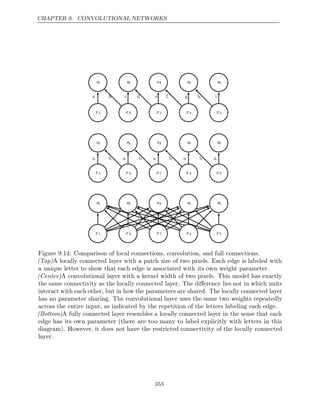
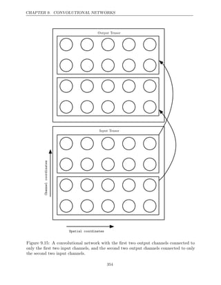
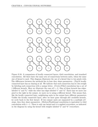
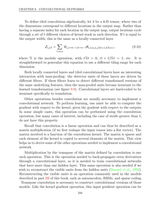
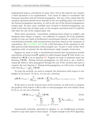
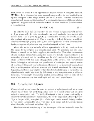
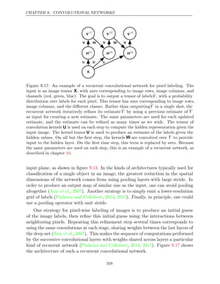
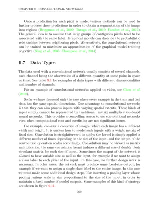
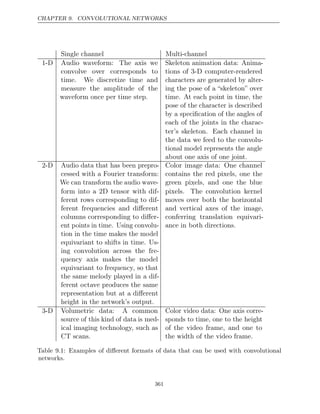
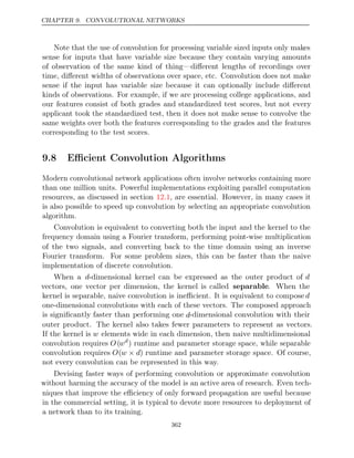
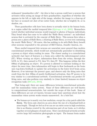
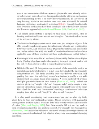
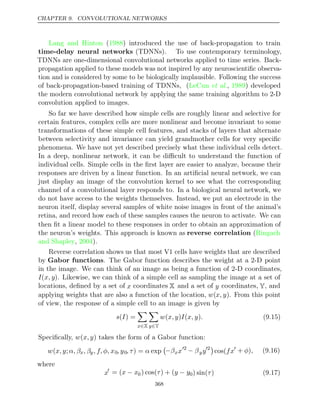
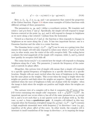
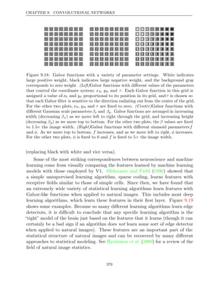
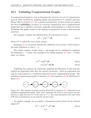
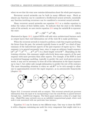
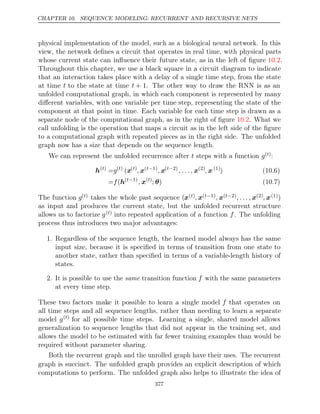
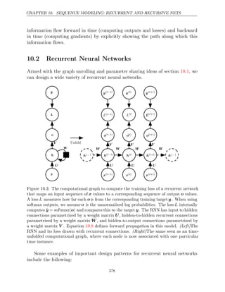
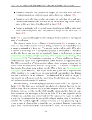
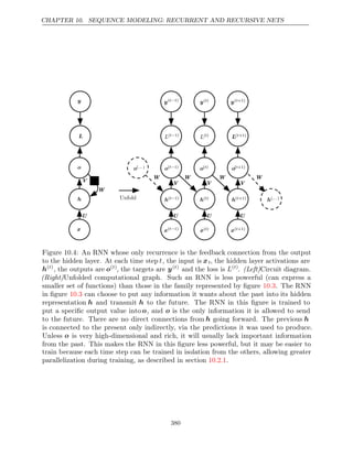
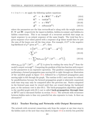
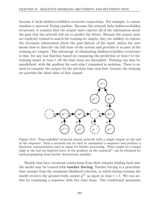
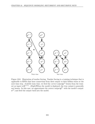
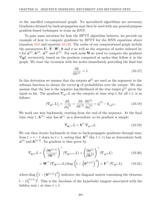
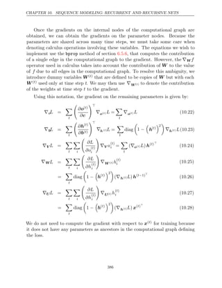
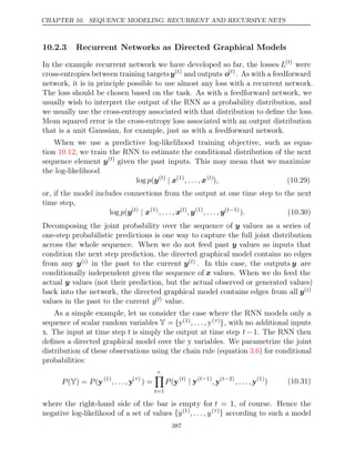
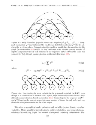
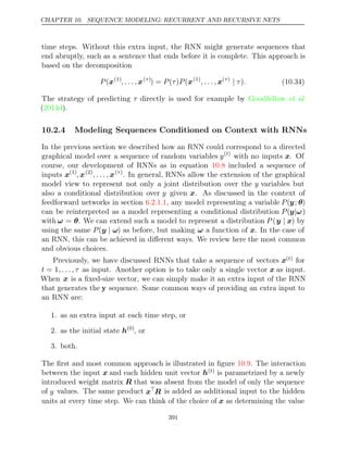
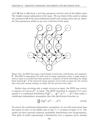
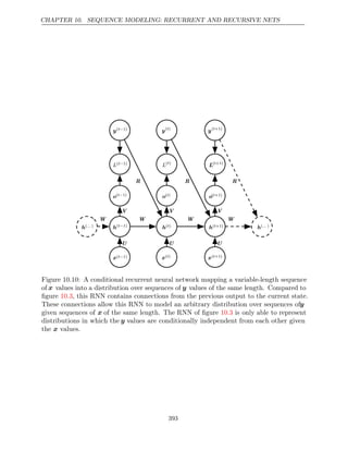
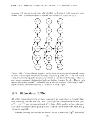
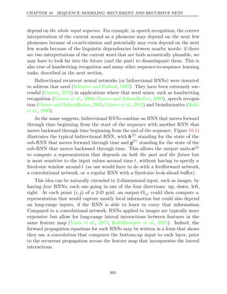
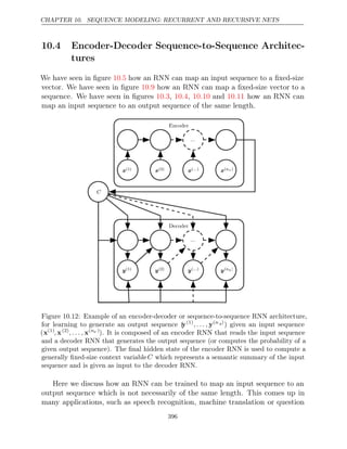
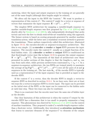
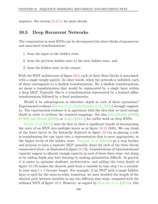
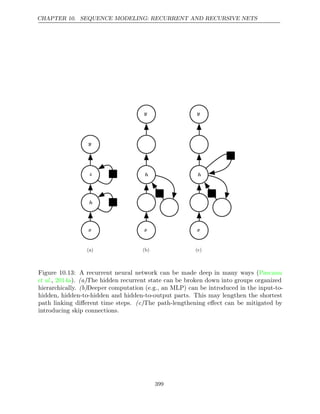
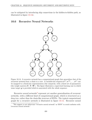
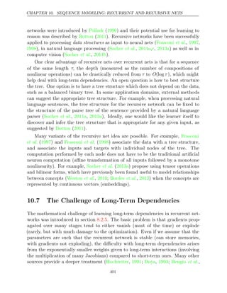
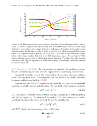
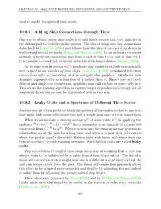
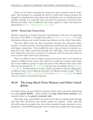
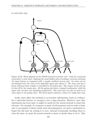
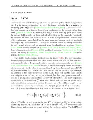
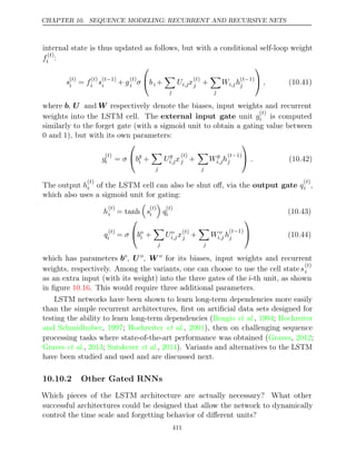
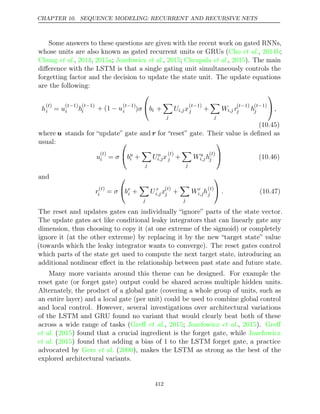
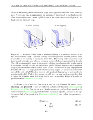
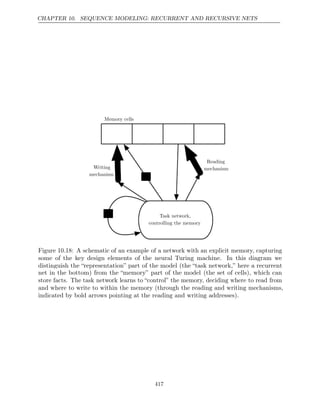
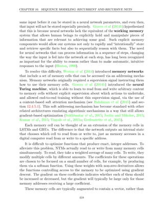
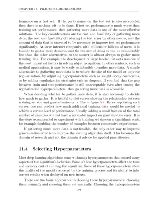
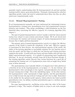
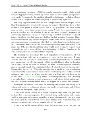
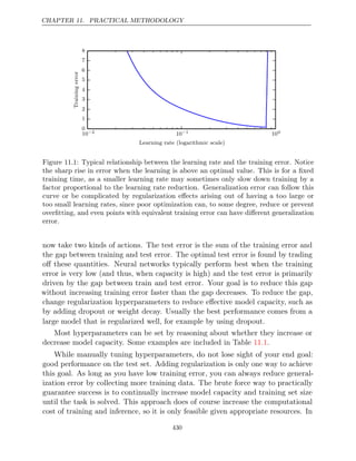
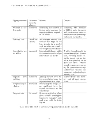
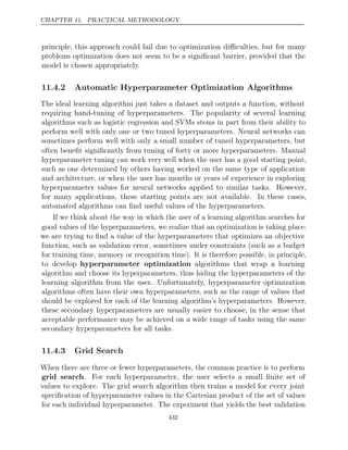
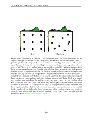
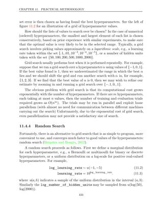
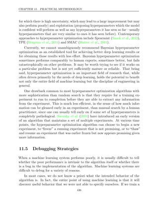
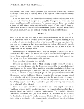
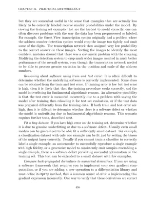
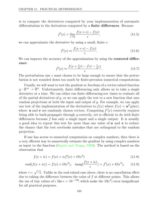
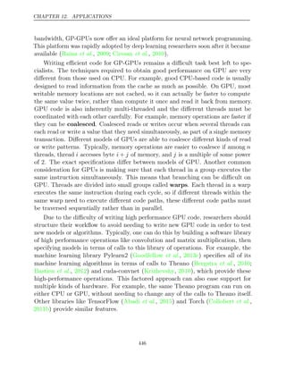
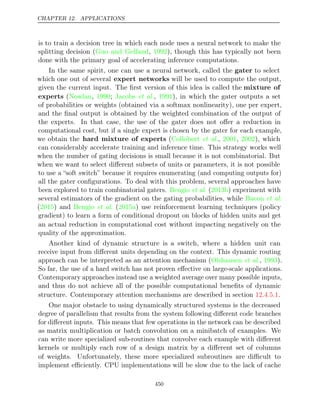
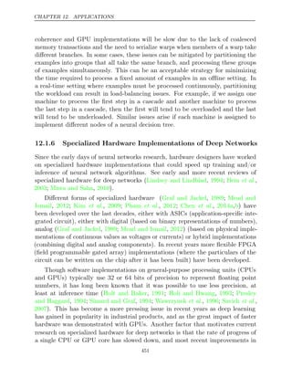
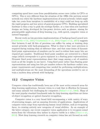
![CHAPTER 12. APPLICATIONS
exotic applications that expand the realm of what is possible with imagery but
rather a small core of AI goals aimed at replicating human abilities. Most deep
learning for computer vision is used for object recognition or detection of some
form, whether this means reporting which object is present in an image, annotating
an image with bounding boxes around each object, transcribing a sequence of
symbols from an image, or labeling each pixel in an image with the identity of the
object it belongs to. Because generative modeling has been a guiding principle
of deep learning research, there is also a large body of work on image synthesis
using deep models. While image synthesis is usually not considered a
ex nihilo
computer vision endeavor, models capable of image synthesis are usually useful for
image restoration, a computer vision task involving repairing defects in images or
removing objects from images.
12.2.1 Preprocessing
Many application areas require sophisticated preprocessing because the original
input comes in a form that is difficult for many deep learning architectures to
represent. Computer vision usually requires relatively little of this kind of pre-
processing. The images should be standardized so that their pixels all lie in the
same, reasonable range, like [0,1] or [-1, 1]. Mixing images that lie in [0,1] with
images that lie in [0, 255] will usually result in failure. Formatting images to have
the same scale is the only kind of preprocessing that is strictly necessary. Many
computer vision architectures require images of a standard size, so images must be
cropped or scaled to fit that size. Even this rescaling is not always strictly necessary.
Some convolutional models accept variably-sized inputs and dynamically adjust
the size of their pooling regions to keep the output size constant (Waibel et al.,
1989). Other convolutional models have variable-sized output that automatically
scales in size with the input, such as models that denoise or label each pixel in an
image ( , ).
Hadsell et al. 2007
Dataset augmentation may be seen as a way of preprocessing the training set
only. Dataset augmentation is an excellent way to reduce the generalization error
of most computer vision models. A related idea applicable at test time is to show
the model many different versions of the same input (for example, the same image
cropped at slightly different locations) and have the different instantiations of the
model vote to determine the output. This latter idea can be interpreted as an
ensemble approach, and helps to reduce generalization error.
Other kinds of preprocessing are applied to both the train and the test set with
the goal of putting each example into a more canonical form in order to reduce the
amount of variation that the model needs to account for. Reducing the amount of
453](https://image.slidesharecdn.com/deeplearningadaptivecomputationandmachinelearningpdfdrive-230402121325-7c74bca2/85/Deep-learning_-adaptive-computation-and-machine-learning-PDFDrive-pdf-469-320.jpg)
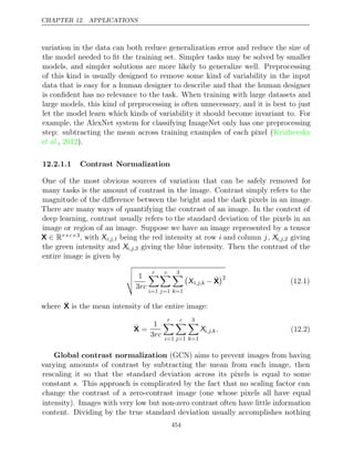
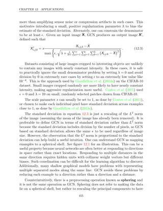
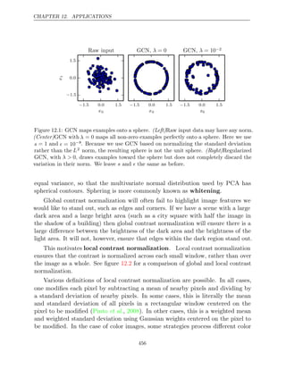
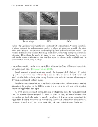
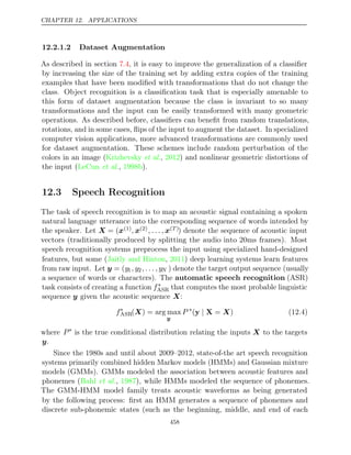
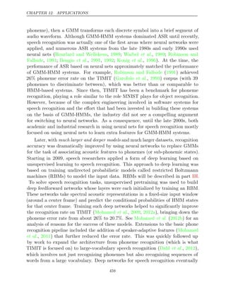
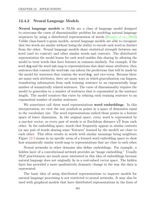
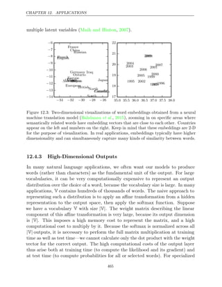
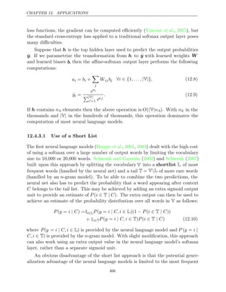
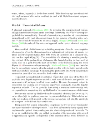
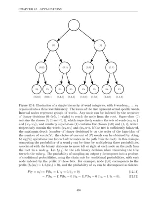
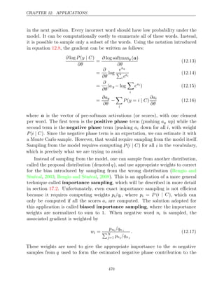
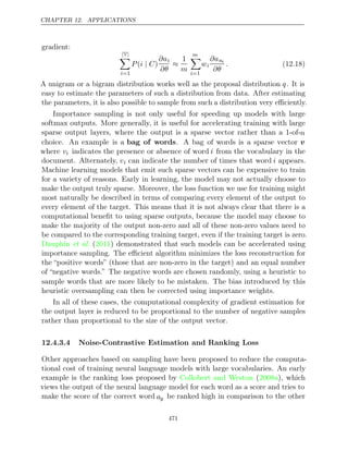
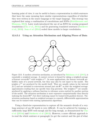
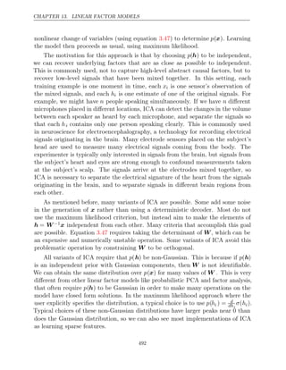
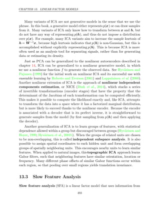
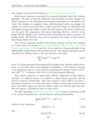
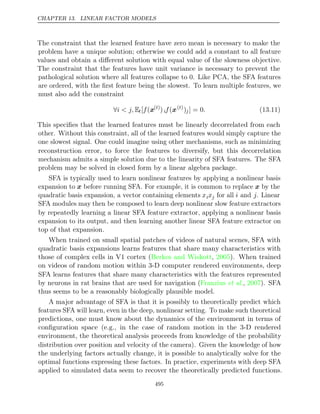
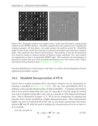
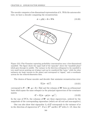
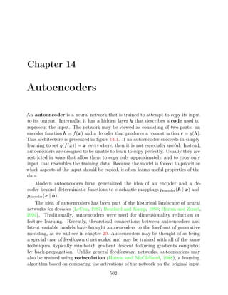
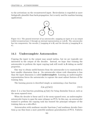
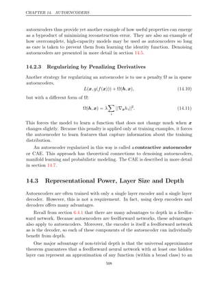
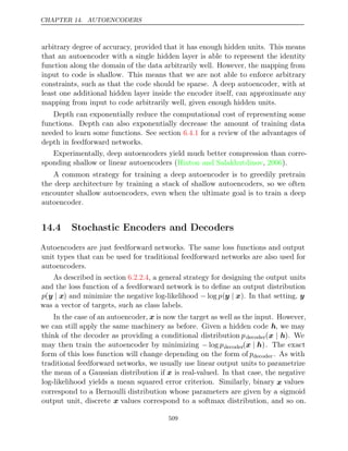
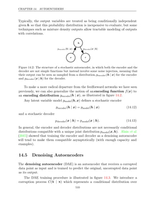
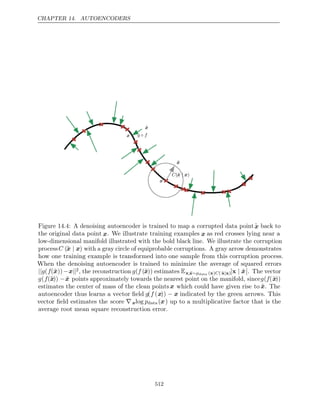
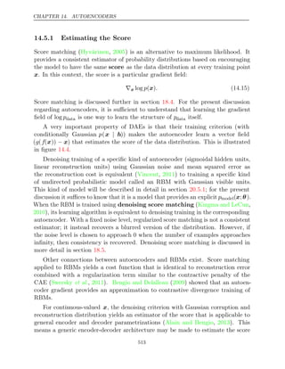
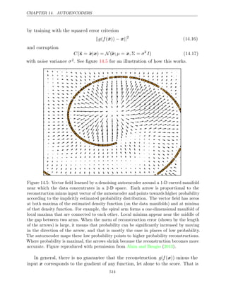
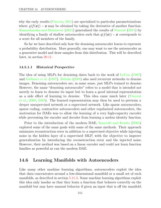
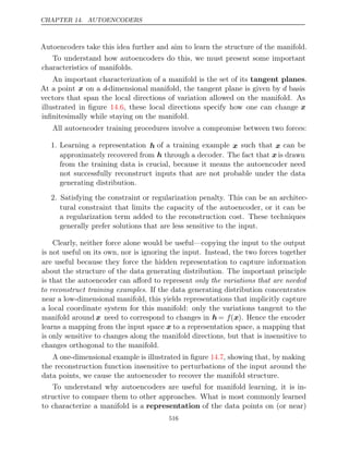
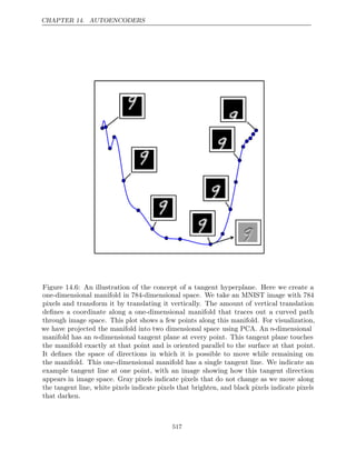
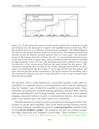
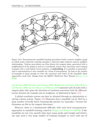
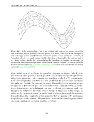
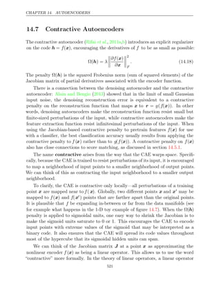
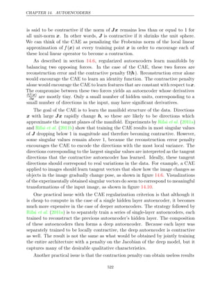
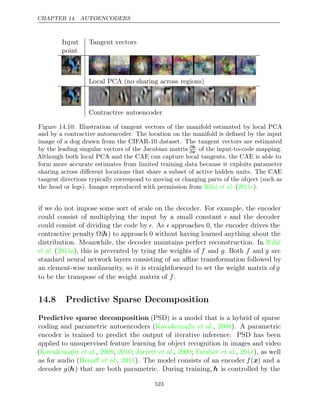
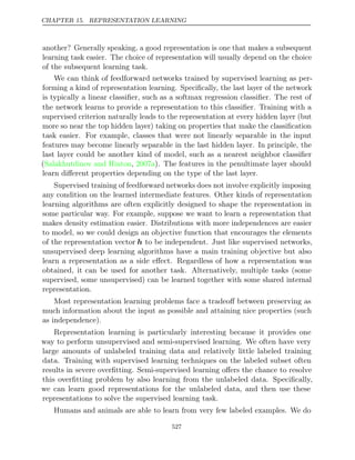
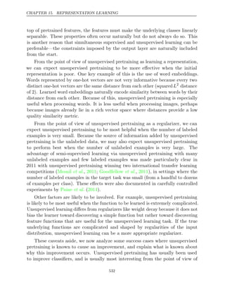
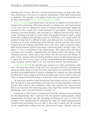
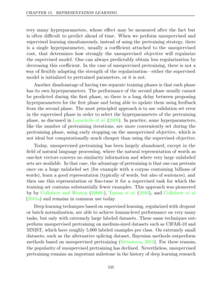
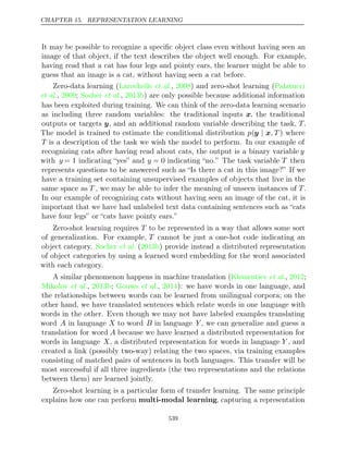
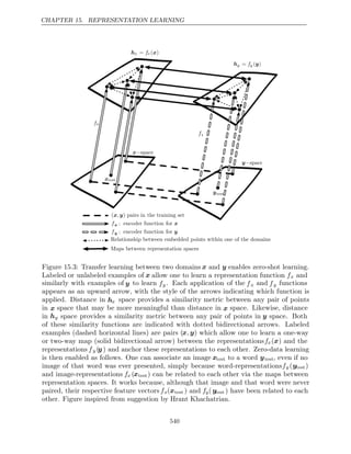
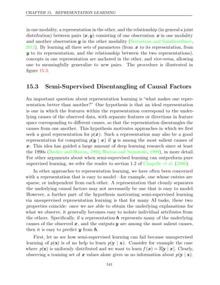
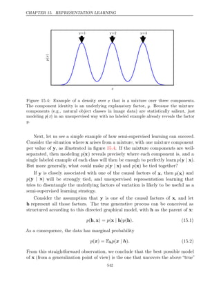
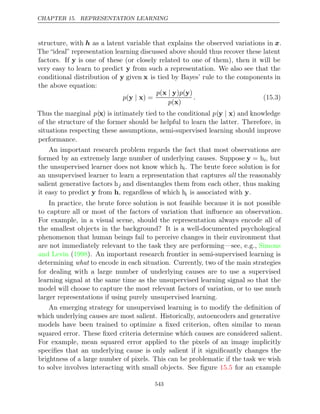
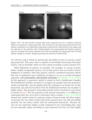
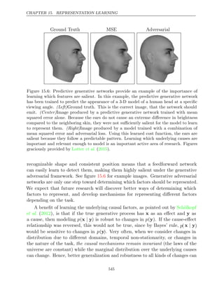
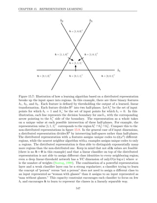
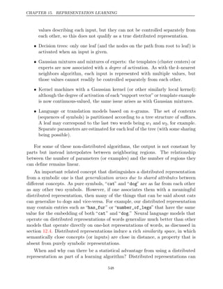
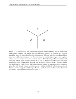
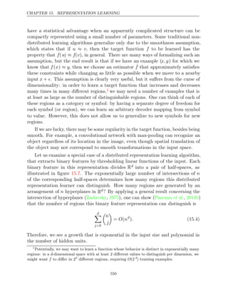
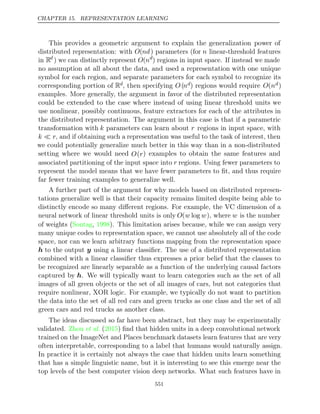
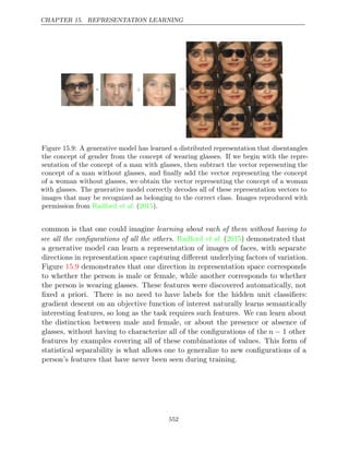
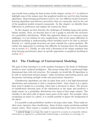
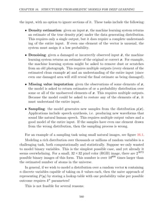
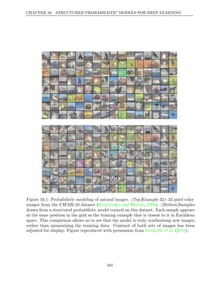

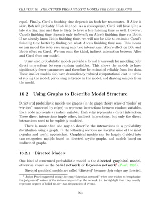
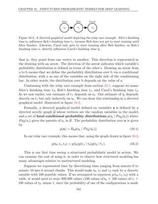
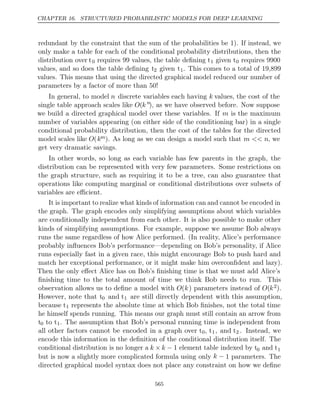
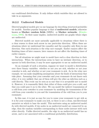
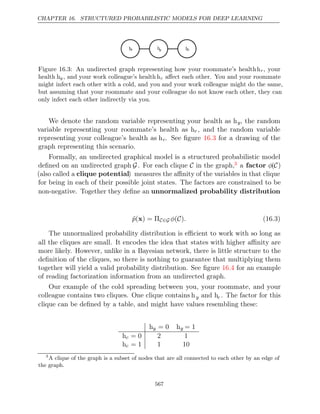
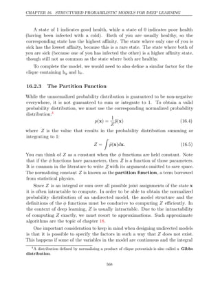
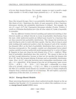
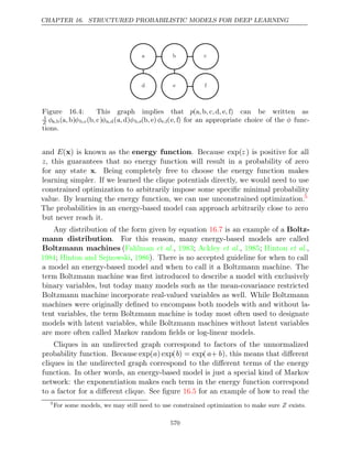
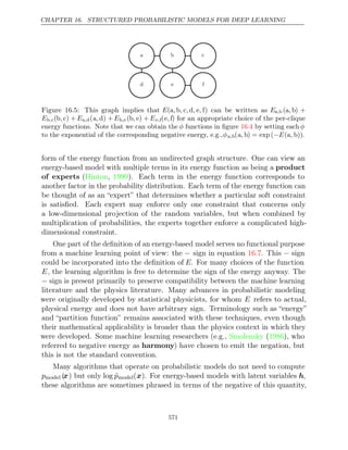
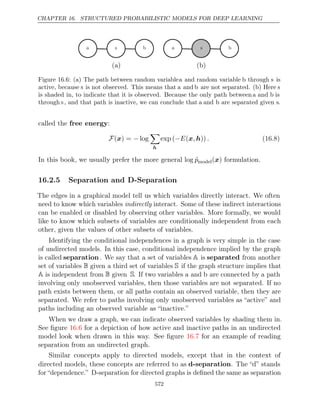
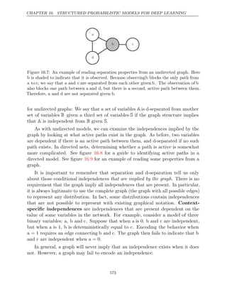
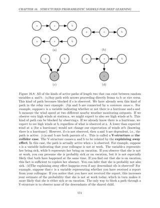
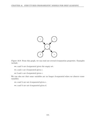
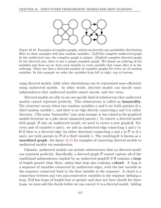
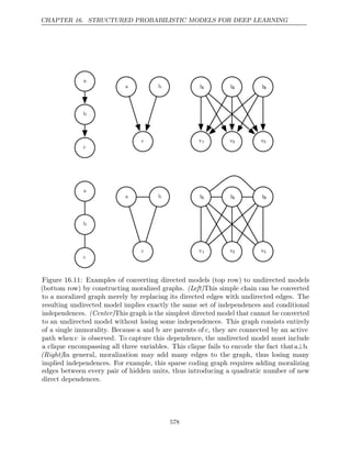
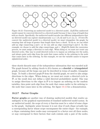
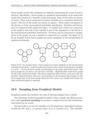
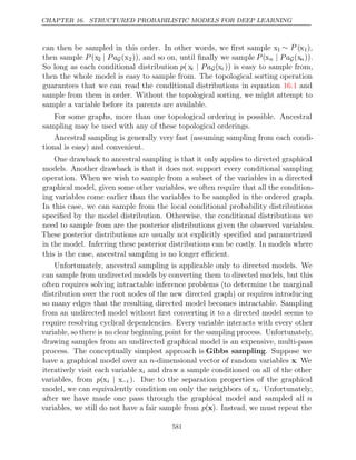
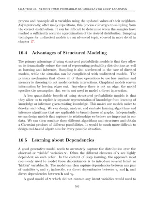
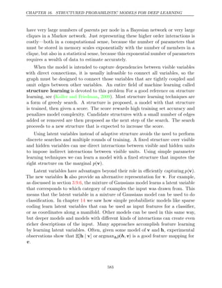
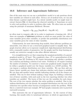
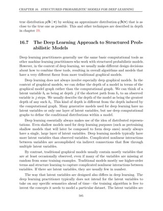
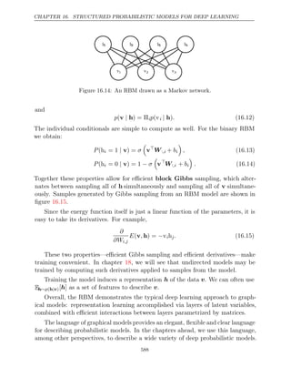
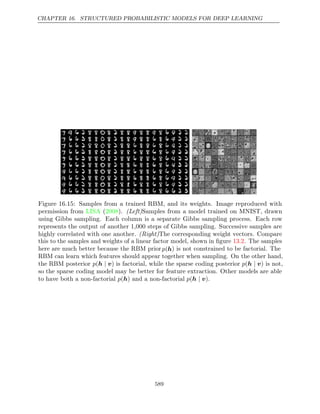
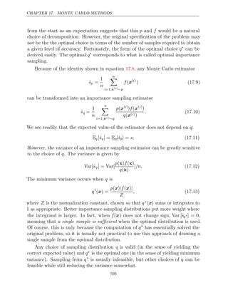
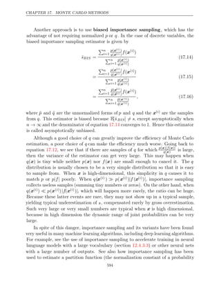
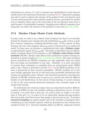
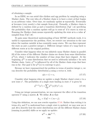
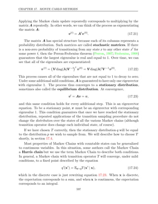
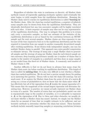
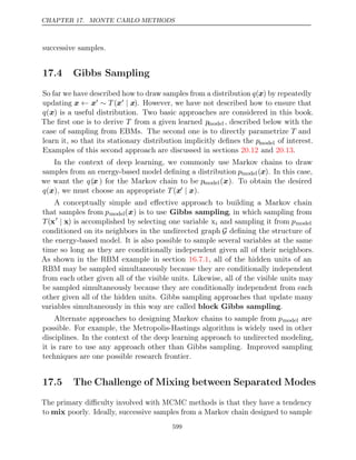
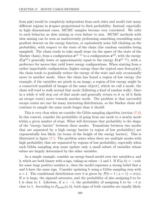
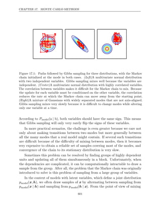
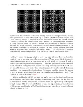
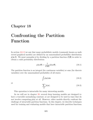
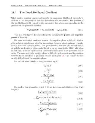
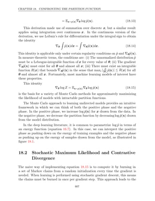
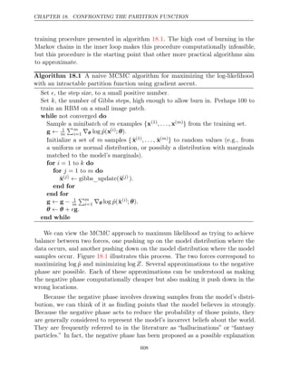
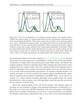
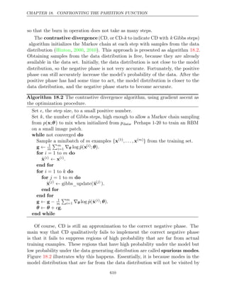
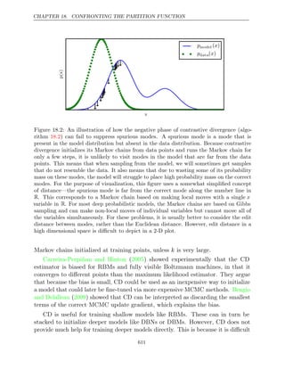
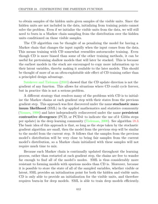
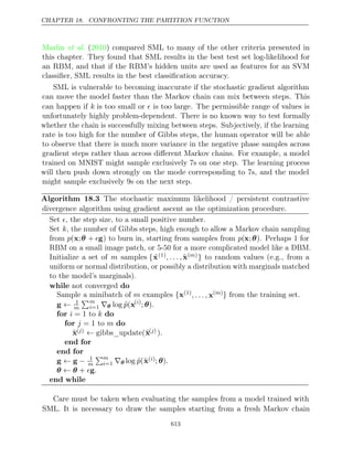
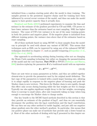
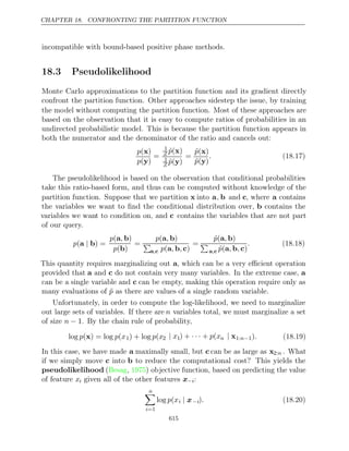
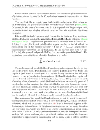
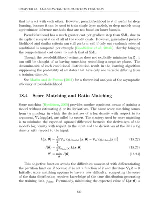
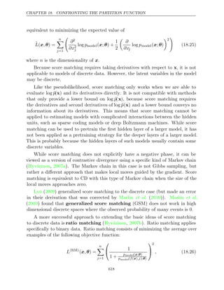
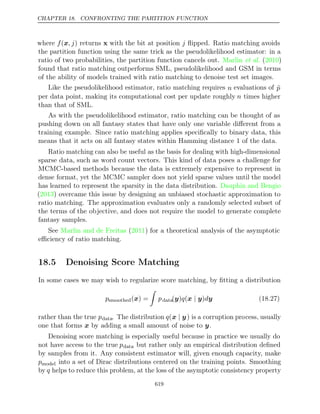
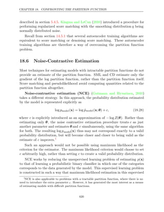
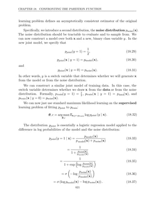
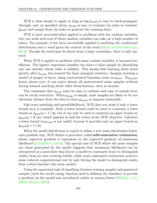
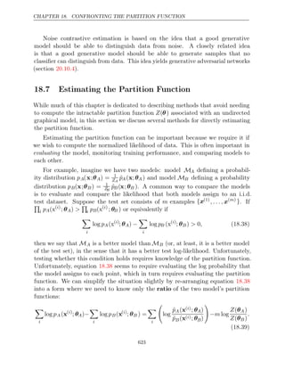
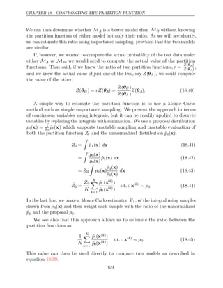
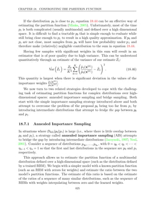
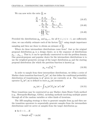
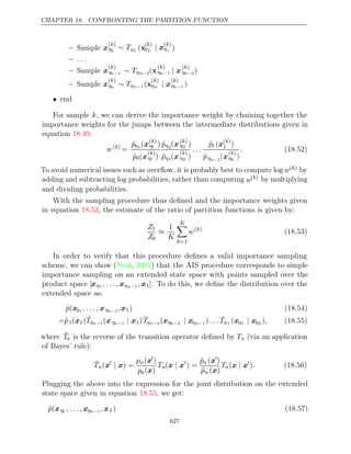
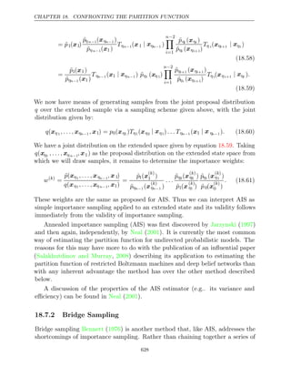
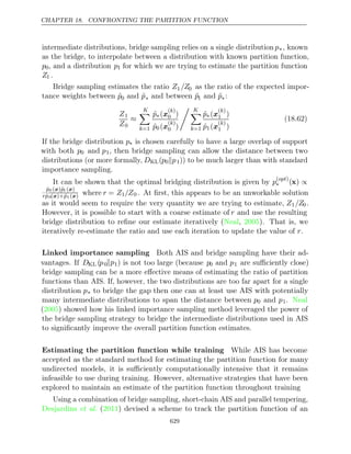
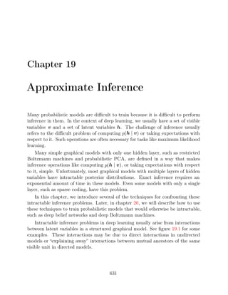
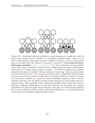
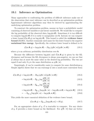
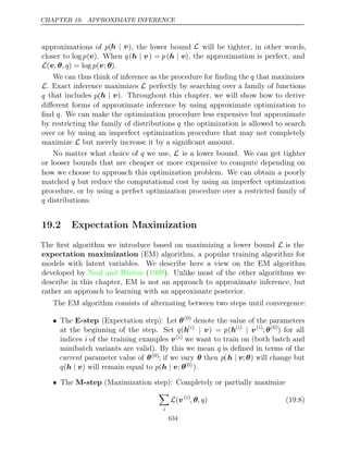
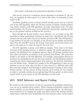
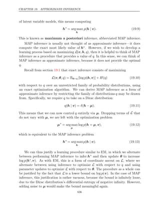
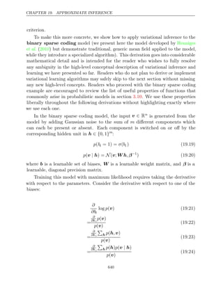
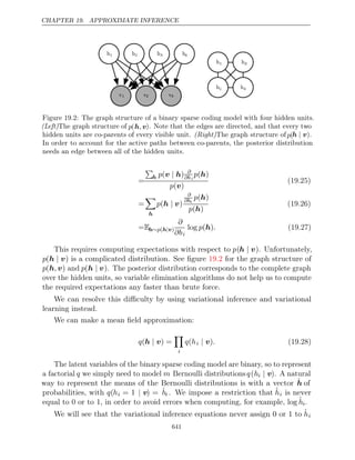
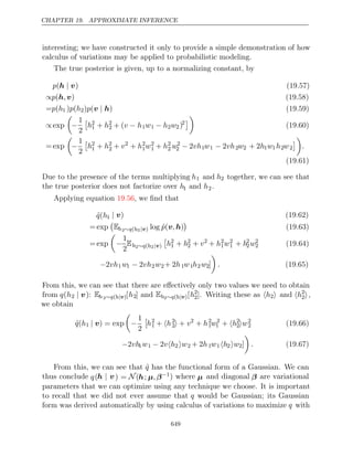
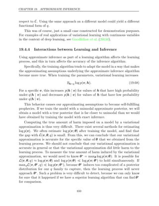
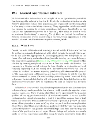
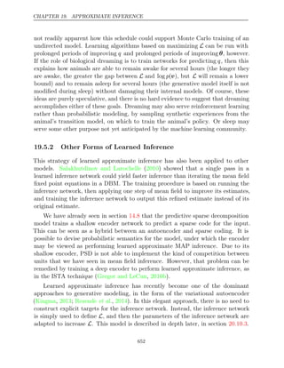

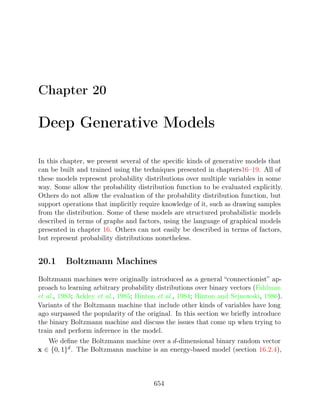
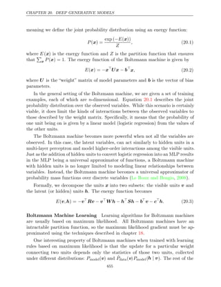
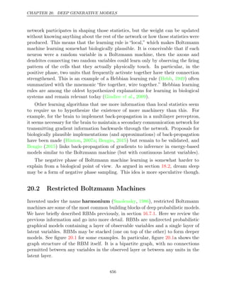
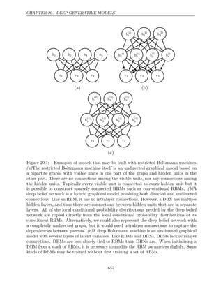
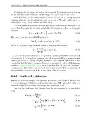
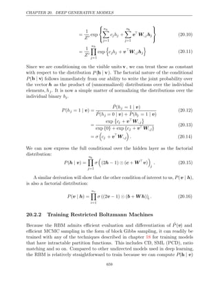
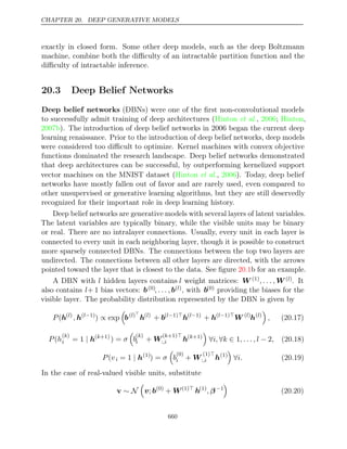
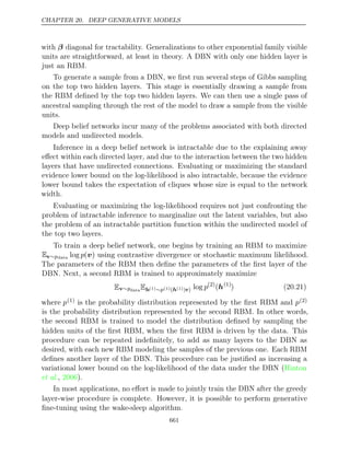
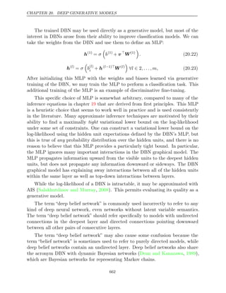
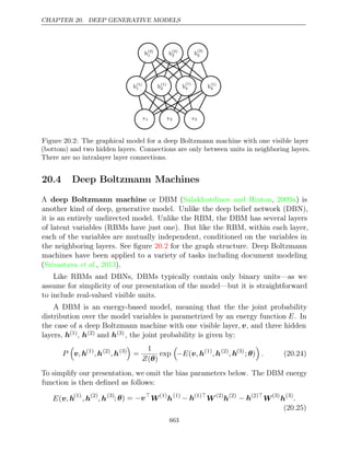
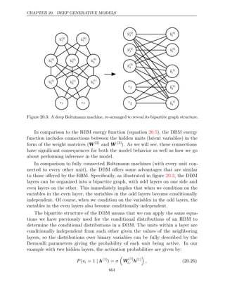
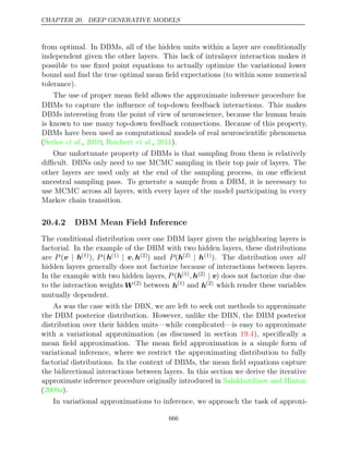
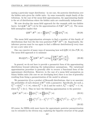
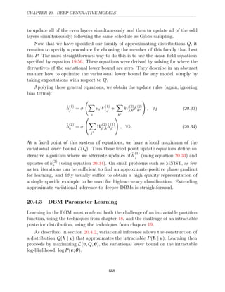
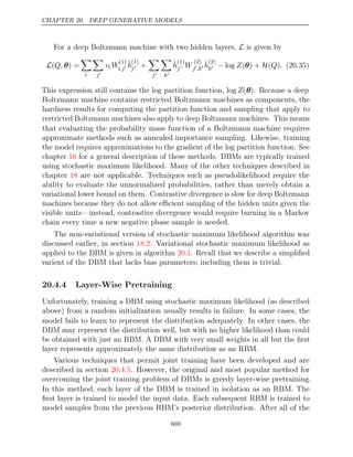
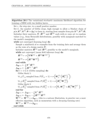
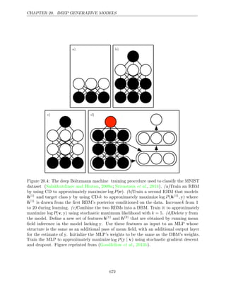
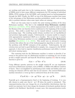
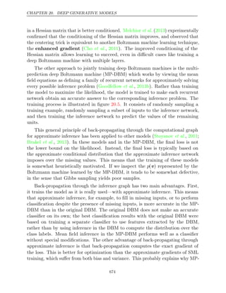
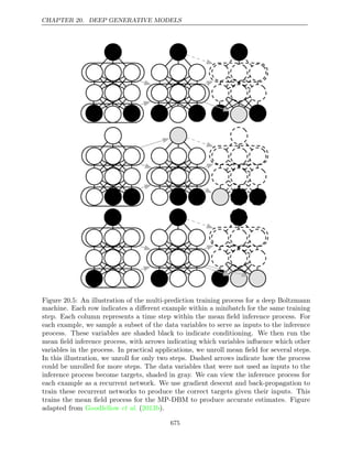
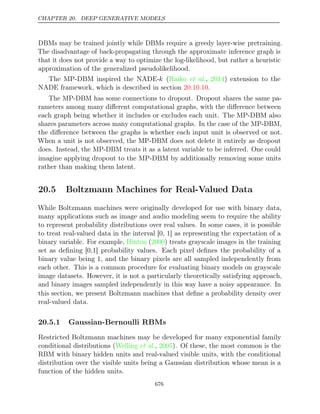
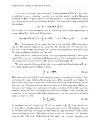
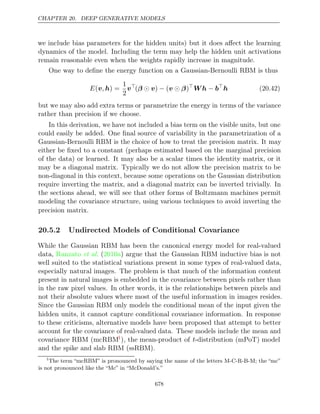
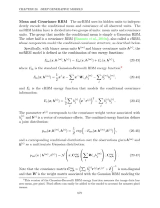
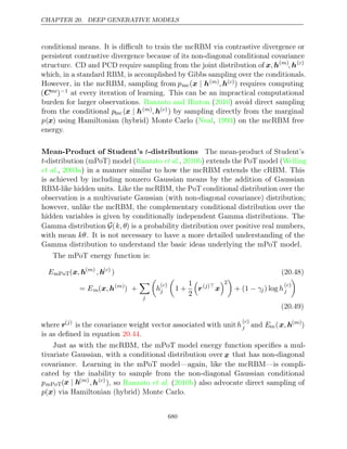
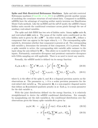
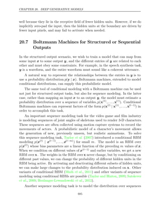
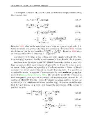
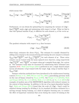
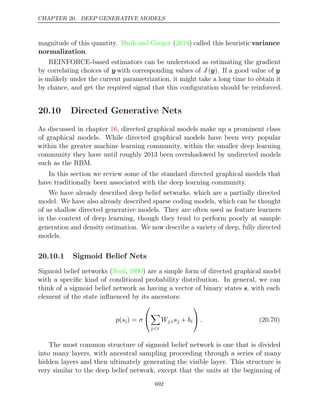
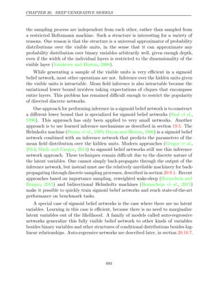
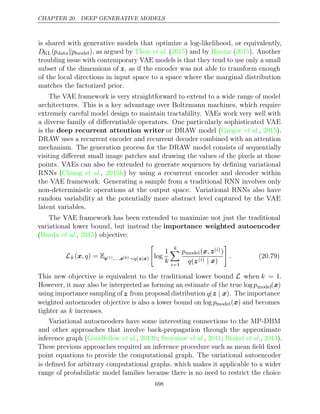
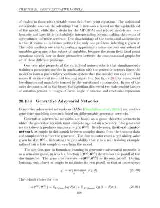
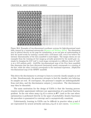
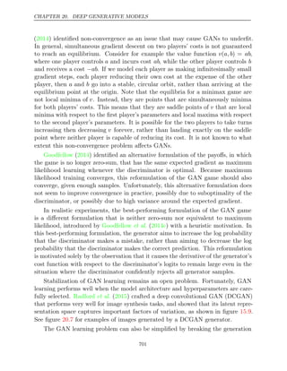
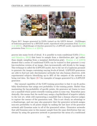
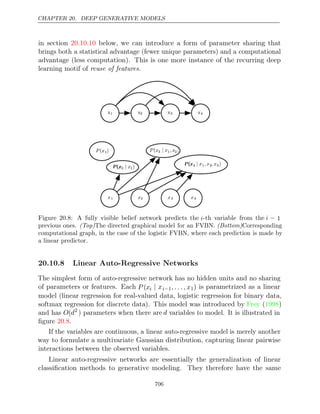
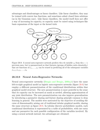
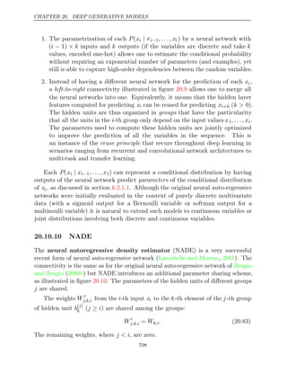
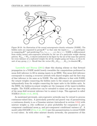
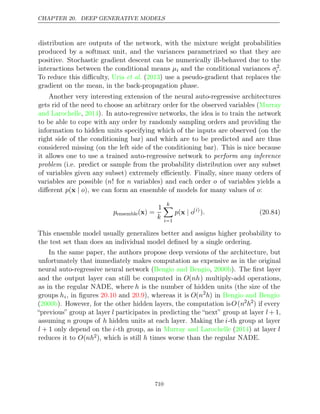
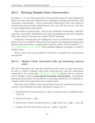
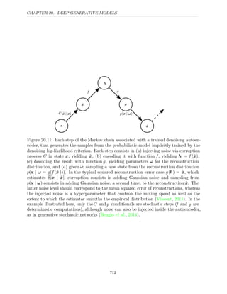
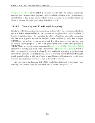
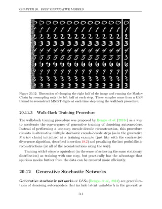
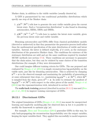
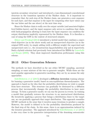
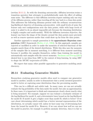
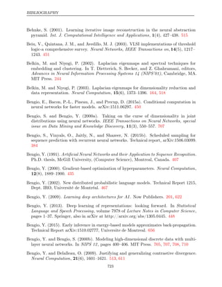
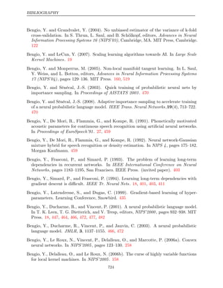
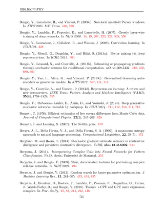
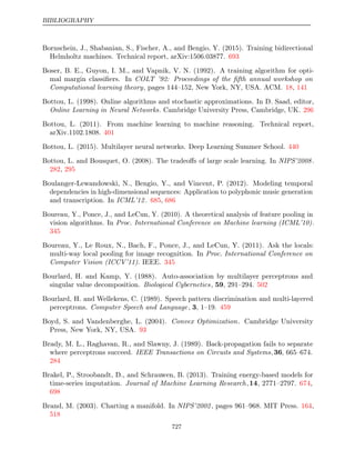
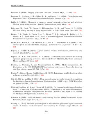
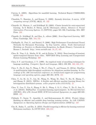
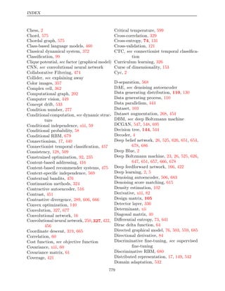
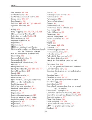
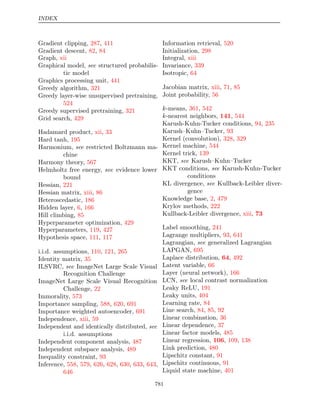

This document provides a table of contents for a book on deep learning. The book covers topics such as linear algebra, probability, machine learning basics, deep feedforward networks, regularization techniques, optimization methods, convolutional networks, sequence modeling and practical applications of deep learning. It is authored by Ian Goodfellow, Yoshua Bengio and Aaron Courville and contains three parts that progress from applied math concepts to modern deep learning practices to current research areas.