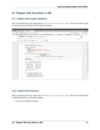
This document is a tutorial for learning Apache Spark with Python. It covers topics like configuring Spark on different platforms, an introduction to Spark's core concepts and architecture, and programming with RDDs. It then demonstrates various machine learning techniques in Spark like regression, classification, clustering, and neural networks. It also discusses automating Spark pipelines and packaging PySpark code.


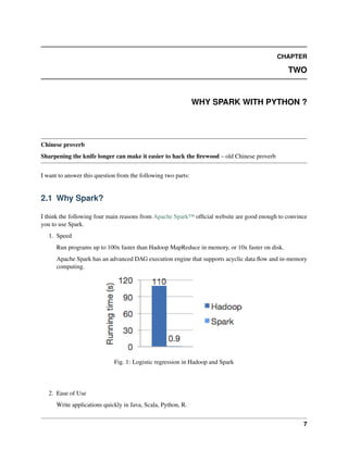
![CHAPTER
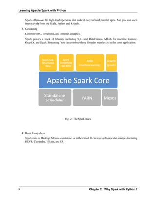
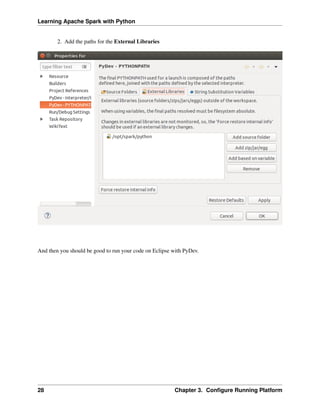
ONE
PREFACE
1.1 About
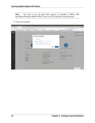
1.1.1 About this note
This is a shared repository for Learning Apache Spark Notes. The PDF version can be downloaded from
HERE. The first version was posted on Github in ChenFeng ([Feng2017]). This shared repository mainly
contains the self-learning and self-teaching notes from Wenqiang during his IMA Data Science Fellowship.
The reader is referred to the repository https://github.com/runawayhorse001/LearningApacheSpark for more
details about the dataset and the .ipynb files.
In this repository, I try to use the detailed demo code and examples to show how to use each main functions.
If you find your work wasn’t cited in this note, please feel free to let me know.
Although I am by no means an data mining programming and Big Data expert, I decided that it would be
useful for me to share what I learned about PySpark programming in the form of easy tutorials with detailed
example. I hope those tutorials will be a valuable tool for your studies.
The tutorials assume that the reader has a preliminary knowledge of programming and Linux. And this
document is generated automatically by using sphinx.
1.1.2 About the author
• Wenqiang Feng
– Director of Data Science and PhD in Mathematics
– University of Tennessee at Knoxville
– Email: von198@gmail.com
• Biography
Wenqiang Feng is the Director of Data Science at American Express (AMEX). Prior to his time at
AMEX, Dr. Feng was a Sr. Data Scientist in Machine Learning Lab, H&R Block. Before joining
Block, Dr. Feng was a Data Scientist at Applied Analytics Group, DST (now SS&C). Dr. Feng’s
responsibilities include providing clients with access to cutting-edge skills and technologies, including
Big Data analytic solutions, advanced analytic and data enhancement techniques and modeling.
3](https://image.slidesharecdn.com/pyspark-230429134708-b35c8a19/85/pyspark-pdf-9-320.jpg)


![Learning Apache Spark with Python
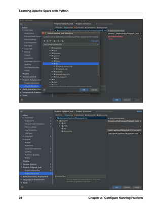
You can check if your Java is available and find it’s version by using the following command in Command
Prompt:
java -version
If your Java is installed successfully, you will get the similar results as follows:
java version "1.8.0_131"
Java(TM) SE Runtime Environment (build 1.8.0_131-b11)
Java HotSpot(TM) 64-Bit Server VM (build 25.131-b11, mixed mode)
3.2.4 Install Apache Spark
Actually, the Pre-build version doesn’t need installation. You can use it when you unpack it.
a. Download: You can get the Pre-built Apache Spark™ from Download Apache Spark™.
b. Unpack: Unpack the Apache Spark™ to the path where you want to install the Spark.
c. Test: Test the Prerequisites: change the direction spark-#.#.#-bin-hadoop#.#/
bin and run
./pyspark
Python 2.7.13 |Anaconda 4.4.0 (x86_64)| (default, Dec 20 2016,
˓
→23:05:08)
[GCC 4.2.1 Compatible Apple LLVM 6.0 (clang-600.0.57)] on darwin
Type "help", "copyright", "credits" or "license" for more
˓
→information.
Anaconda is brought to you by Continuum Analytics.
Please check out: http://continuum.io/thanks and https://anaconda.org
Using Spark's default log4j profile: org/apache/spark/log4j-defaults.
˓
→properties
Setting default log level to "WARN".
To adjust logging level use sc.setLogLevel(newLevel). For SparkR,
use setLogLevel(newLevel).
17/08/30 13:30:12 WARN NativeCodeLoader: Unable to load native-hadoop
library for your platform... using builtin-java classes where
˓
→applicable
17/08/30 13:30:17 WARN ObjectStore: Failed to get database global_
˓
→temp,
returning NoSuchObjectException
Welcome to
____ __
/ __/__ ___ _____/ /__
_ / _ / _ `/ __/ '_/
/__ / .__/_,_/_/ /_/_ version 2.1.1
/_/
Using Python version 2.7.13 (default, Dec 20 2016 23:05:08)
SparkSession available as 'spark'.
3.2. Configure Spark on Mac and Ubuntu 19](https://image.slidesharecdn.com/pyspark-230429134708-b35c8a19/85/pyspark-pdf-25-320.jpg)


![Learning Apache Spark with Python
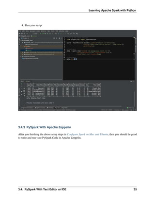
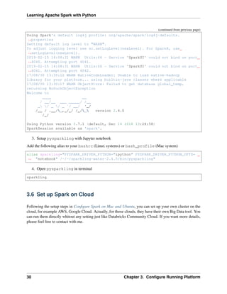
3.5 PySparkling Water: Spark + H2O
1. Download Sparkling Water from: https://s3.amazonaws.com/h2o-release/sparkling-water/
rel-2.4/5/index.html
2. Test PySparking
unzip sparkling-water-2.4.5.zip
cd ~/sparkling-water-2.4.5/bin
./pysparkling
If you have a correct setup for PySpark, then you will get the following results:
Using Spark defined in the SPARK_HOME=/Users/dt216661/spark environmental
˓
→property
Python 3.7.1 (default, Dec 14 2018, 13:28:58)
[GCC 4.2.1 Compatible Apple LLVM 6.0 (clang-600.0.57)] on darwin
Type "help", "copyright", "credits" or "license" for more information.
2019-02-15 14:08:30 WARN NativeCodeLoader:62 - Unable to load native-hadoop
˓
→library for your platform... using builtin-java classes where applicable
Setting default log level to "WARN".
(continues on next page)
3.5. PySparkling Water: Spark + H2O 29](https://image.slidesharecdn.com/pyspark-230429134708-b35c8a19/85/pyspark-pdf-35-320.jpg)
![Learning Apache Spark with Python
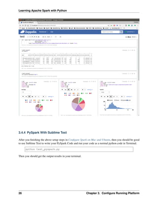
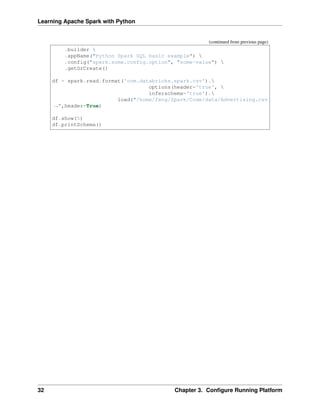
3.7 PySpark on Colaboratory
Colaboratory is a free Jupyter notebook environment that requires no setup and runs entirely in the cloud.
3.7.1 Installation
!pip install pyspark
3.7.2 Testing
from pyspark.sql import SparkSession
spark = SparkSession
.builder
.appName("Python Spark create RDD example")
.config("spark.some.config.option", "some-value")
.getOrCreate()
df = spark.sparkContext
.parallelize([(1, 2, 3, 'a b c'),
(4, 5, 6, 'd e f'),
(7, 8, 9, 'g h i')])
.toDF(['col1', 'col2', 'col3','col4'])
df.show()
Output:
+----+----+----+-----+
|col1|col2|col3| col4|
+----+----+----+-----+
| 1| 2| 3|a b c|
| 4| 5| 6|d e f|
| 7| 8| 9|g h i|
+----+----+----+-----+
3.8 Demo Code in this Section
The Jupyter notebook can be download from installation on colab.
• Python Source code
## set up SparkSession
from pyspark.sql import SparkSession
spark = SparkSession
(continues on next page)
3.7. PySpark on Colaboratory 31](https://image.slidesharecdn.com/pyspark-230429134708-b35c8a19/85/pyspark-pdf-37-320.jpg)
![CHAPTER
FOUR
AN INTRODUCTION TO APACHE SPARK
Chinese proverb
Know yourself and know your enemy, and you will never be defeated – idiom, from Sunzi’s Art of War
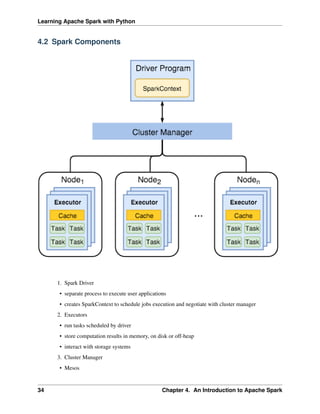
4.1 Core Concepts
Most of the following content comes from [Kirillov2016]. So the copyright belongs to Anton Kirillov. I
will refer you to get more details from Apache Spark core concepts, architecture and internals.
Before diving deep into how Apache Spark works, lets understand the jargon of Apache Spark
• Job: A piece of code which reads some input from HDFS or local, performs some computation on the
data and writes some output data.
• Stages: Jobs are divided into stages. Stages are classified as a Map or reduce stages (Its easier to
understand if you have worked on Hadoop and want to correlate). Stages are divided based on com-
putational boundaries, all computations (operators) cannot be Updated in a single Stage. It happens
over many stages.
• Tasks: Each stage has some tasks, one task per partition. One task is executed on one partition of data
on one executor (machine).
• DAG: DAG stands for Directed Acyclic Graph, in the present context its a DAG of operators.
• Executor: The process responsible for executing a task.
• Master: The machine on which the Driver program runs
• Slave: The machine on which the Executor program runs
33](https://image.slidesharecdn.com/pyspark-230429134708-b35c8a19/85/pyspark-pdf-39-320.jpg)
![CHAPTER
FIVE
PROGRAMMING WITH RDDS
Chinese proverb
If you only know yourself, but not your opponent, you may win or may lose. If you know neither
yourself nor your enemy, you will always endanger yourself – idiom, from Sunzi’s Art of War
RDD represents Resilient Distributed Dataset. An RDD in Spark is simply an immutable distributed
collection of objects sets. Each RDD is split into multiple partitions (similar pattern with smaller sets),
which may be computed on different nodes of the cluster.
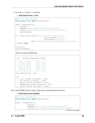
5.1 Create RDD
Usually, there are two popular ways to create the RDDs: loading an external dataset, or distributing a
set of collection of objects. The following examples show some simplest ways to create RDDs by using
parallelize() fucntion which takes an already existing collection in your program and pass the same
to the Spark Context.
1. By using parallelize( ) function
from pyspark.sql import SparkSession
spark = SparkSession
.builder
.appName("Python Spark create RDD example")
.config("spark.some.config.option", "some-value")
.getOrCreate()
df = spark.sparkContext.parallelize([(1, 2, 3, 'a b c'),
(4, 5, 6, 'd e f'),
(7, 8, 9, 'g h i')]).toDF(['col1', 'col2', 'col3','col4'])
Then you will get the RDD data:
df.show()
+----+----+----+-----+
(continues on next page)
37](https://image.slidesharecdn.com/pyspark-230429134708-b35c8a19/85/pyspark-pdf-43-320.jpg)
![Learning Apache Spark with Python
(continued from previous page)
|col1|col2|col3| col4|
+----+----+----+-----+
| 1| 2| 3|a b c|
| 4| 5| 6|d e f|
| 7| 8| 9|g h i|
+----+----+----+-----+
from pyspark.sql import SparkSession
spark = SparkSession
.builder
.appName("Python Spark create RDD example")
.config("spark.some.config.option", "some-value")
.getOrCreate()
myData = spark.sparkContext.parallelize([(1,2), (3,4), (5,6), (7,8), (9,10)])
Then you will get the RDD data:
myData.collect()
[(1, 2), (3, 4), (5, 6), (7, 8), (9, 10)]
2. By using createDataFrame( ) function
from pyspark.sql import SparkSession
spark = SparkSession
.builder
.appName("Python Spark create RDD example")
.config("spark.some.config.option", "some-value")
.getOrCreate()
Employee = spark.createDataFrame([
('1', 'Joe', '70000', '1'),
('2', 'Henry', '80000', '2'),
('3', 'Sam', '60000', '2'),
('4', 'Max', '90000', '1')],
['Id', 'Name', 'Sallary','DepartmentId']
)
Then you will get the RDD data:
+---+-----+-------+------------+
| Id| Name|Sallary|DepartmentId|
+---+-----+-------+------------+
| 1| Joe| 70000| 1|
| 2|Henry| 80000| 2|
| 3| Sam| 60000| 2|
| 4| Max| 90000| 1|
+---+-----+-------+------------+
38 Chapter 5. Programming with RDDs](https://image.slidesharecdn.com/pyspark-230429134708-b35c8a19/85/pyspark-pdf-44-320.jpg)
![Learning Apache Spark with Python
(continued from previous page)
sc= SparkContext('local','example')
hc = HiveContext(sc)
tf1 = sc.textFile("hdfs://cdhstltest/user/data/demo.CSV")
print(tf1.first())
hc.sql("use intg_cme_w")
spf = hc.sql("SELECT * FROM spf LIMIT 100")
print(spf.show(5))
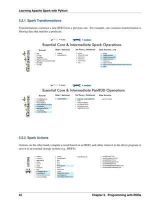
5.2 Spark Operations
Warning: All the figures below are from Jeffrey Thompson. The interested reader is referred to pyspark
pictures
There are two main types of Spark operations: Transformations and Actions [Karau2015].
Note: Some people defined three types of operations: Transformations, Actions and Shuffles.
5.2. Spark Operations 41](https://image.slidesharecdn.com/pyspark-230429134708-b35c8a19/85/pyspark-pdf-47-320.jpg)
![Learning Apache Spark with Python
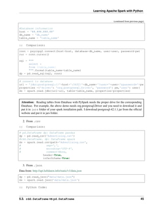
5.3 rdd.DataFrame vs pd.DataFrame
5.3.1 Create DataFrame
1. From List
my_list = [['a', 1, 2], ['b', 2, 3],['c', 3, 4]]
col_name = ['A', 'B', 'C']
:: Python Code:
# caution for the columns=
pd.DataFrame(my_list,columns= col_name)
#
spark.createDataFrame(my_list, col_name).show()
:: Comparison:
+---+---+---+
| A| B| C|
A B C +---+---+---+
0 a 1 2 | a| 1| 2|
1 b 2 3 | b| 2| 3|
2 c 3 4 | c| 3| 4|
+---+---+---+
Attention: Pay attentation to the parameter columns= in pd.DataFrame. Since the default value
will make the list as rows.
:: Python Code:
# caution for the columns=
pd.DataFrame(my_list, columns= col_name)
#
pd.DataFrame(my_list, col_name)
:: Comparison:
5.3. rdd.DataFrame vs pd.DataFrame 43](https://image.slidesharecdn.com/pyspark-230429134708-b35c8a19/85/pyspark-pdf-49-320.jpg)
![Learning Apache Spark with Python
A B C 0 1 2
0 a 1 2 A a 1 2
1 b 2 3 B b 2 3
2 c 3 4 C c 3 4
2. From Dict
d = {'A': [0, 1, 0],
'B': [1, 0, 1],
'C': [1, 0, 0]}
:: Python Code:
pd.DataFrame(d)for
# Tedious for PySpark
spark.createDataFrame(np.array(list(d.values())).T.tolist(),list(d.keys())).
˓
→show()
:: Comparison:
+---+---+---+
| A| B| C|
A B C +---+---+---+
0 0 1 1 | 0| 1| 1|
1 1 0 0 | 1| 0| 0|
2 0 1 0 | 0| 1| 0|
+---+---+---+
5.3.2 Load DataFrame
1. From DataBase
Most of time, you need to share your code with your colleagues or release your code for Code Review or
Quality assurance(QA). You will definitely do not want to have your User Information in the code.
So you can save them in login.txt:
runawayhorse001
PythonTips
and use the following code to import your User Information:
#User Information
try:
login = pd.read_csv(r'login.txt', header=None)
user = login[0][0]
pw = login[0][1]
print('User information is ready!')
except:
print('Login information is not available!!!')
(continues on next page)
44 Chapter 5. Programming with RDDs](https://image.slidesharecdn.com/pyspark-230429134708-b35c8a19/85/pyspark-pdf-50-320.jpg)
![Learning Apache Spark with Python
dp[['id','timestamp']].head(4)
#
ds[['id','timestamp']].show(4)
:: Comparison:
+----------+------------------
˓
→-+
| id|
˓
→timestamp|
id timestamp +----------+------------------
˓
→-+
0 2994551481 2019-02-28 17:23:52 |2994551481|2019-02-28
˓
→17:23:52|
1 2994551482 2019-02-28 17:23:52 |2994551482|2019-02-28
˓
→17:23:52|
2 2994551483 2019-02-28 17:23:52 |2994551483|2019-02-28
˓
→17:23:52|
3 2994551484 2019-02-28 17:23:52 |2994551484|2019-02-28
˓
→17:23:52|
+----------+------------------
˓
→-+
only showing top 4 rows
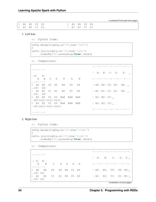
5.3.3 First n Rows
:: Python Code:
dp.head(4)
#
ds.show(4)
:: Comparison:
+-----+-----+---------+-----+
| TV|Radio|Newspaper|Sales|
TV Radio Newspaper Sales +-----+-----+---------+-----+
0 230.1 37.8 69.2 22.1 |230.1| 37.8| 69.2| 22.1|
1 44.5 39.3 45.1 10.4 | 44.5| 39.3| 45.1| 10.4|
2 17.2 45.9 69.3 9.3 | 17.2| 45.9| 69.3| 9.3|
3 151.5 41.3 58.5 18.5 |151.5| 41.3| 58.5| 18.5|
+-----+-----+---------+-----+
only showing top 4 rows
46 Chapter 5. Programming with RDDs](https://image.slidesharecdn.com/pyspark-230429134708-b35c8a19/85/pyspark-pdf-52-320.jpg)
![Learning Apache Spark with Python
5.3.4 Column Names
:: Python Code:
dp.columns
#
ds.columns
:: Comparison:
Index(['TV', 'Radio', 'Newspaper', 'Sales'], dtype='object')
['TV', 'Radio', 'Newspaper', 'Sales']
5.3.5 Data types
:: Python Code:
dp.dtypes
#
ds.dtypes
:: Comparison:
TV float64 [('TV', 'double'),
Radio float64 ('Radio', 'double'),
Newspaper float64 ('Newspaper', 'double'),
Sales float64 ('Sales', 'double')]
dtype: object
5.3.6 Fill Null
my_list = [['male', 1, None], ['female', 2, 3],['male', 3, 4]]
dp = pd.DataFrame(my_list,columns=['A', 'B', 'C'])
ds = spark.createDataFrame(my_list, ['A', 'B', 'C'])
#
dp.head()
ds.show()
:: Comparison:
+------+---+----+
| A| B| C|
A B C +------+---+----+
0 male 1 NaN | male| 1|null|
1 female 2 3.0 |female| 2| 3|
2 male 3 4.0 | male| 3| 4|
+------+---+----+
:: Python Code:
5.3. rdd.DataFrame vs pd.DataFrame 47](https://image.slidesharecdn.com/pyspark-230429134708-b35c8a19/85/pyspark-pdf-53-320.jpg)
![Learning Apache Spark with Python
dp.fillna(-99)
#
ds.fillna(-99).show()
:: Comparison:
+------+---+----+
| A| B| C|
A B C +------+---+----+
0 male 1 -99 | male| 1| -99|
1 female 2 3.0 |female| 2| 3|
2 male 3 4.0 | male| 3| 4|
+------+---+----+
5.3.7 Replace Values
:: Python Code:
# caution: you need to chose specific col
dp.A.replace(['male', 'female'],[1, 0], inplace=True)
dp
#caution: Mixed type replacements are not supported
ds.na.replace(['male','female'],['1','0']).show()
:: Comparison:
+---+---+----+
| A| B| C|
A B C +---+---+----+
0 1 1 NaN | 1| 1|null|
1 0 2 3.0 | 0| 2| 3|
2 1 3 4.0 | 1| 3| 4|
+---+---+----+
5.3.8 Rename Columns
1. Rename all columns
:: Python Code:
dp.columns = ['a','b','c','d']
dp.head(4)
#
ds.toDF('a','b','c','d').show(4)
:: Comparison:
+-----+----+----+----+
| a| b| c| d|
(continues on next page)
48 Chapter 5. Programming with RDDs](https://image.slidesharecdn.com/pyspark-230429134708-b35c8a19/85/pyspark-pdf-54-320.jpg)
![Learning Apache Spark with Python
(continued from previous page)
a b c d +-----+----+----+----+
0 230.1 37.8 69.2 22.1 |230.1|37.8|69.2|22.1|
1 44.5 39.3 45.1 10.4 | 44.5|39.3|45.1|10.4|
2 17.2 45.9 69.3 9.3 | 17.2|45.9|69.3| 9.3|
3 151.5 41.3 58.5 18.5 |151.5|41.3|58.5|18.5|
+-----+----+----+----+
only showing top 4 rows
2. Rename one or more columns
mapping = {'Newspaper':'C','Sales':'D'}
:: Python Code:
dp.rename(columns=mapping).head(4)
#
new_names = [mapping.get(col,col) for col in ds.columns]
ds.toDF(*new_names).show(4)
:: Comparison:
+-----+-----+----+----+
| TV|Radio| C| D|
TV Radio C D +-----+-----+----+----+
0 230.1 37.8 69.2 22.1 |230.1| 37.8|69.2|22.1|
1 44.5 39.3 45.1 10.4 | 44.5| 39.3|45.1|10.4|
2 17.2 45.9 69.3 9.3 | 17.2| 45.9|69.3| 9.3|
3 151.5 41.3 58.5 18.5 |151.5| 41.3|58.5|18.5|
+-----+-----+----+----+
only showing top 4 rows
Note: You can also use withColumnRenamed to rename one column in PySpark.
:: Python Code:
ds.withColumnRenamed('Newspaper','Paper').show(4
:: Comparison:
+-----+-----+-----+-----+
| TV|Radio|Paper|Sales|
+-----+-----+-----+-----+
|230.1| 37.8| 69.2| 22.1|
| 44.5| 39.3| 45.1| 10.4|
| 17.2| 45.9| 69.3| 9.3|
|151.5| 41.3| 58.5| 18.5|
+-----+-----+-----+-----+
only showing top 4 rows
5.3. rdd.DataFrame vs pd.DataFrame 49](https://image.slidesharecdn.com/pyspark-230429134708-b35c8a19/85/pyspark-pdf-55-320.jpg)
![Learning Apache Spark with Python
5.3.9 Drop Columns
drop_name = ['Newspaper','Sales']
:: Python Code:
dp.drop(drop_name,axis=1).head(4)
#
ds.drop(*drop_name).show(4)
:: Comparison:
+-----+-----+
| TV|Radio|
TV Radio +-----+-----+
0 230.1 37.8 |230.1| 37.8|
1 44.5 39.3 | 44.5| 39.3|
2 17.2 45.9 | 17.2| 45.9|
3 151.5 41.3 |151.5| 41.3|
+-----+-----+
only showing top 4 rows
5.3.10 Filter
dp = pd.read_csv('Advertising.csv')
#
ds = spark.read.csv(path='Advertising.csv',
header=True,
inferSchema=True)
:: Python Code:
dp[dp.Newspaper<20].head(4)
#
ds[ds.Newspaper<20].show(4)
:: Comparison:
+-----+-----+---------+-----+
| TV|Radio|Newspaper|Sales|
TV Radio Newspaper Sales +-----+-----+---------+-----+
7 120.2 19.6 11.6 13.2 |120.2| 19.6| 11.6| 13.2|
8 8.6 2.1 1.0 4.8 | 8.6| 2.1| 1.0| 4.8|
11 214.7 24.0 4.0 17.4 |214.7| 24.0| 4.0| 17.4|
13 97.5 7.6 7.2 9.7 | 97.5| 7.6| 7.2| 9.7|
+-----+-----+---------+-----+
only showing top 4 rows
:: Python Code:
50 Chapter 5. Programming with RDDs](https://image.slidesharecdn.com/pyspark-230429134708-b35c8a19/85/pyspark-pdf-56-320.jpg)
![Learning Apache Spark with Python
dp[(dp.Newspaper<20)&(dp.TV>100)].head(4)
#
ds[(ds.Newspaper<20)&(ds.TV>100)].show(4)
:: Comparison:
+-----+-----+---------+-----+
| TV|Radio|Newspaper|Sales|
TV Radio Newspaper Sales +-----+-----+---------+-----+
7 120.2 19.6 11.6 13.2 |120.2| 19.6| 11.6| 13.2|
11 214.7 24.0 4.0 17.4 |214.7| 24.0| 4.0| 17.4|
19 147.3 23.9 19.1 14.6 |147.3| 23.9| 19.1| 14.6|
25 262.9 3.5 19.5 12.0 |262.9| 3.5| 19.5| 12.0|
+-----+-----+---------+-----+
only showing top 4 rows
5.3.11 With New Column
:: Python Code:
dp['tv_norm'] = dp.TV/sum(dp.TV)
dp.head(4)
#
ds.withColumn('tv_norm', ds.TV/ds.groupBy().agg(F.sum("TV")).collect()[0][0]).
˓
→show(4)
:: Comparison:
+-----+-----+---------+-----+-
˓
→-------------------+
| TV|Radio|Newspaper|Sales|
˓
→ tv_norm|
TV Radio Newspaper Sales tv_norm +-----+-----+---------+-----+-
˓
→-------------------+
0 230.1 37.8 69.2 22.1 0.007824 |230.1| 37.8| 69.2| 22.
˓
→1|0.007824268493802813|
1 44.5 39.3 45.1 10.4 0.001513 | 44.5| 39.3| 45.1| 10.
˓
→4|0.001513167961643...|
2 17.2 45.9 69.3 9.3 0.000585 | 17.2| 45.9| 69.3| 9.
˓
→3|5.848649200061207E-4|
3 151.5 41.3 58.5 18.5 0.005152 |151.5| 41.3| 58.5| 18.
˓
→5|0.005151571824472517|
+-----+-----+---------+-----+-
˓
→-------------------+
only showing top 4 rows
:: Python Code:
5.3. rdd.DataFrame vs pd.DataFrame 51](https://image.slidesharecdn.com/pyspark-230429134708-b35c8a19/85/pyspark-pdf-57-320.jpg)
![Learning Apache Spark with Python
dp['cond'] = dp.apply(lambda c: 1 if ((c.TV>100)&(c.Radio<40)) else 2 if c.
˓
→Sales> 10 else 3,axis=1)
#
ds.withColumn('cond',F.when((ds.TV>100)&(ds.Radio<40),1)
.when(ds.Sales>10, 2)
.otherwise(3)).show(4)
:: Comparison:
+-----+-----+---------+-----+-
˓
→---+
|
˓
→TV|Radio|Newspaper|Sales|cond|
TV Radio Newspaper Sales cond +-----+-----+---------+-----+-
˓
→---+
0 230.1 37.8 69.2 22.1 1 |230.1| 37.8| 69.2| 22.1|
˓
→ 1|
1 44.5 39.3 45.1 10.4 2 | 44.5| 39.3| 45.1| 10.4|
˓
→ 2|
2 17.2 45.9 69.3 9.3 3 | 17.2| 45.9| 69.3| 9.3|
˓
→ 3|
3 151.5 41.3 58.5 18.5 2 |151.5| 41.3| 58.5| 18.5|
˓
→ 2|
+-----+-----+---------+-----+-
˓
→---+
only showing top 4 rows
:: Python Code:
dp['log_tv'] = np.log(dp.TV)
dp.head(4)
#
import pyspark.sql.functions as F
ds.withColumn('log_tv',F.log(ds.TV)).show(4)
:: Comparison:
+-----+-----+---------+-----+-
˓
→-----------------+
| TV|Radio|Newspaper|Sales|
˓
→ log_tv|
TV Radio Newspaper Sales log_tv +-----+-----+---------+-----+-
˓
→-----------------+
0 230.1 37.8 69.2 22.1 5.438514 |230.1| 37.8| 69.2| 22.1|
˓
→ 5.43851399704132|
1 44.5 39.3 45.1 10.4 3.795489 | 44.5| 39.3| 45.1| 10.
˓
→4|3.7954891891721947|
2 17.2 45.9 69.3 9.3 2.844909 | 17.2| 45.9| 69.3| 9.
˓
→3|2.8449093838194073|
3 151.5 41.3 58.5 18.5 5.020586 |151.5| 41.3| 58.5| 18.5|
˓
→5.020585624949423|
+-----+-----+---------+-----+-
˓
→-----------------+ (continues on next page)
52 Chapter 5. Programming with RDDs](https://image.slidesharecdn.com/pyspark-230429134708-b35c8a19/85/pyspark-pdf-58-320.jpg)
![Learning Apache Spark with Python
(continued from previous page)
only showing top 4 rows
:: Python Code:
dp['tv+10'] = dp.TV.apply(lambda x: x+10)
dp.head(4)
#
ds.withColumn('tv+10', ds.TV+10).show(4)
:: Comparison:
+-----+-----+---------+-----+-
˓
→----+
|
˓
→TV|Radio|Newspaper|Sales|tv+10|
TV Radio Newspaper Sales tv+10 +-----+-----+---------+-----+-
˓
→----+
0 230.1 37.8 69.2 22.1 240.1 |230.1| 37.8| 69.2| 22.
˓
→1|240.1|
1 44.5 39.3 45.1 10.4 54.5 | 44.5| 39.3| 45.1| 10.4|
˓
→54.5|
2 17.2 45.9 69.3 9.3 27.2 | 17.2| 45.9| 69.3| 9.3|
˓
→27.2|
3 151.5 41.3 58.5 18.5 161.5 |151.5| 41.3| 58.5| 18.
˓
→5|161.5|
+-----+-----+---------+-----+-
˓
→----+
only showing top 4 rows
5.3.12 Join
leftp = pd.DataFrame({'A': ['A0', 'A1', 'A2', 'A3'],
'B': ['B0', 'B1', 'B2', 'B3'],
'C': ['C0', 'C1', 'C2', 'C3'],
'D': ['D0', 'D1', 'D2', 'D3']},
index=[0, 1, 2, 3])
rightp = pd.DataFrame({'A': ['A0', 'A1', 'A6', 'A7'],
'F': ['B4', 'B5', 'B6', 'B7'],
'G': ['C4', 'C5', 'C6', 'C7'],
'H': ['D4', 'D5', 'D6', 'D7']},
index=[4, 5, 6, 7])
lefts = spark.createDataFrame(leftp)
rights = spark.createDataFrame(rightp)
A B C D A F G H
0 A0 B0 C0 D0 4 A0 B4 C4 D4
1 A1 B1 C1 D1 5 A1 B5 C5 D5
(continues on next page)
5.3. rdd.DataFrame vs pd.DataFrame 53](https://image.slidesharecdn.com/pyspark-230429134708-b35c8a19/85/pyspark-pdf-59-320.jpg)
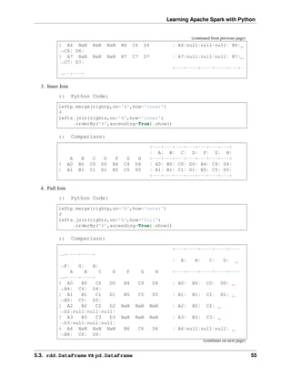
![Learning Apache Spark with Python
(continued from previous page)
5 A7 NaN NaN NaN B7 C7 D7 | A7|null|null|null|
˓
→B7| C7| D7|
+---+----+----+----+----
˓
→+----+----+
5.3.13 Concat Columns
my_list = [('a', 2, 3),
('b', 5, 6),
('c', 8, 9),
('a', 2, 3),
('b', 5, 6),
('c', 8, 9)]
col_name = ['col1', 'col2', 'col3']
#
dp = pd.DataFrame(my_list,columns=col_name)
ds = spark.createDataFrame(my_list,schema=col_name)
col1 col2 col3
0 a 2 3
1 b 5 6
2 c 8 9
3 a 2 3
4 b 5 6
5 c 8 9
:: Python Code:
dp['concat'] = dp.apply(lambda x:'%s%s'%(x['col1'],x['col2']),axis=1)
dp
#
ds.withColumn('concat',F.concat('col1','col2')).show()
:: Comparison:
+----+----+----+------+
|col1|col2|col3|concat|
col1 col2 col3 concat +----+----+----+------+
0 a 2 3 a2 | a| 2| 3| a2|
1 b 5 6 b5 | b| 5| 6| b5|
2 c 8 9 c8 | c| 8| 9| c8|
3 a 2 3 a2 | a| 2| 3| a2|
4 b 5 6 b5 | b| 5| 6| b5|
5 c 8 9 c8 | c| 8| 9| c8|
+----+----+----+------+
56 Chapter 5. Programming with RDDs](https://image.slidesharecdn.com/pyspark-230429134708-b35c8a19/85/pyspark-pdf-62-320.jpg)
![Learning Apache Spark with Python
5.3.14 GroupBy
:: Python Code:
dp.groupby(['col1']).agg({'col2':'min','col3':'mean'})
#
ds.groupBy(['col1']).agg({'col2': 'min', 'col3': 'avg'}).show()
:: Comparison:
+----+---------+---------+
col2 col3 |col1|min(col2)|avg(col3)|
col1 +----+---------+---------+
a 2 3 | c| 8| 9.0|
b 5 6 | b| 5| 6.0|
c 8 9 | a| 2| 3.0|
+----+---------+---------+
5.3.15 Pivot
:: Python Code:
pd.pivot_table(dp, values='col3', index='col1', columns='col2', aggfunc=np.
˓
→sum)
#
ds.groupBy(['col1']).pivot('col2').sum('col3').show()
:: Comparison:
+----+----+----+----+
col2 2 5 8 |col1| 2| 5| 8|
col1 +----+----+----+----+
a 6.0 NaN NaN | c|null|null| 18|
b NaN 12.0 NaN | b|null| 12|null|
c NaN NaN 18.0 | a| 6|null|null|
+----+----+----+----+
5.3.16 Window
d = {'A':['a','b','c','d'],'B':['m','m','n','n'],'C':[1,2,3,6]}
dp = pd.DataFrame(d)
ds = spark.createDataFrame(dp)
:: Python Code:
dp['rank'] = dp.groupby('B')['C'].rank('dense',ascending=False)
#
from pyspark.sql.window import Window
(continues on next page)
5.3. rdd.DataFrame vs pd.DataFrame 57](https://image.slidesharecdn.com/pyspark-230429134708-b35c8a19/85/pyspark-pdf-63-320.jpg)
![Learning Apache Spark with Python
(continued from previous page)
w = Window.partitionBy('B').orderBy(ds.C.desc())
ds = ds.withColumn('rank',F.rank().over(w))
:: Comparison:
+---+---+---+----+
| A| B| C|rank|
A B C rank +---+---+---+----+
0 a m 1 2.0 | b| m| 2| 1|
1 b m 2 1.0 | a| m| 1| 2|
2 c n 3 2.0 | d| n| 6| 1|
3 d n 6 1.0 | c| n| 3| 2|
+---+---+---+----+
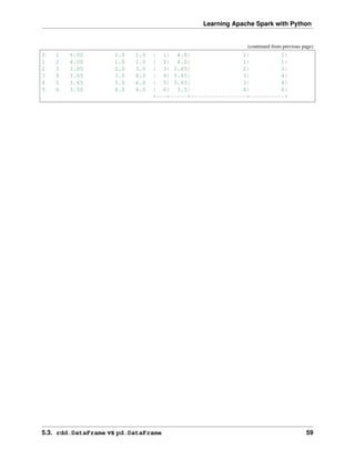
5.3.17 rank vs dense_rank
d ={'Id':[1,2,3,4,5,6],
'Score': [4.00, 4.00, 3.85, 3.65, 3.65, 3.50]}
#
data = pd.DataFrame(d)
dp = data.copy()
ds = spark.createDataFrame(data)
Id Score
0 1 4.00
1 2 4.00
2 3 3.85
3 4 3.65
4 5 3.65
5 6 3.50
:: Python Code:
dp['Rank_dense'] = dp['Score'].rank(method='dense',ascending =False)
dp['Rank'] = dp['Score'].rank(method='min',ascending =False)
dp
#
import pyspark.sql.functions as F
from pyspark.sql.window import Window
w = Window.orderBy(ds.Score.desc())
ds = ds.withColumn('Rank_spark_dense',F.dense_rank().over(w))
ds = ds.withColumn('Rank_spark',F.rank().over(w))
ds.show()
:: Comparison:
+---+-----+----------------+----------+
| Id|Score|Rank_spark_dense|Rank_spark|
Id Score Rank_dense Rank +---+-----+----------------+----------+
(continues on next page)
58 Chapter 5. Programming with RDDs](https://image.slidesharecdn.com/pyspark-230429134708-b35c8a19/85/pyspark-pdf-64-320.jpg)

![CHAPTER
SIX
STATISTICS AND LINEAR ALGEBRA PRELIMINARIES
Chinese proverb
If you only know yourself, but not your opponent, you may win or may lose. If you know neither
yourself nor your enemy, you will always endanger yourself – idiom, from Sunzi’s Art of War
6.1 Notations
• m : the number of the samples
• n : the number of the features
• 𝑦𝑖 : i-th label
• ˆ
𝑦𝑖 : i-th predicted label
• ¯
𝑦 = 1
𝑚
∑︀𝑚
𝑖=1 𝑦𝑖 : the mean of 𝑦.
• 𝑦 : the label vector.
• ˆ
𝑦 : the predicted label vector.
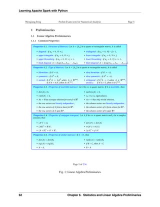
6.2 Linear Algebra Preliminaries
Since I have documented the Linear Algebra Preliminaries in my Prelim Exam note for Numerical Analysis,
the interested reader is referred to [Feng2014] for more details (Figure. Linear Algebra Preliminaries).
61](https://image.slidesharecdn.com/pyspark-230429134708-b35c8a19/85/pyspark-pdf-67-320.jpg)

![Learning Apache Spark with Python
7.1.1 Numerical Variables
Describe
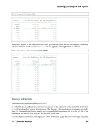
The describe function in pandas and spark will give us most of the statistical results, such as min,
median, max, quartiles and standard deviation. With the help of the user defined function,
you can get even more statistical results.
# selected varables for the demonstration
num_cols = ['Account Balance','No of dependents']
df.select(num_cols).describe().show()
+-------+------------------+-------------------+
|summary| Account Balance| No of dependents|
+-------+------------------+-------------------+
| count| 1000| 1000|
| mean| 2.577| 1.155|
| stddev|1.2576377271108936|0.36208577175319395|
| min| 1| 1|
| max| 4| 2|
+-------+------------------+-------------------+
You may find out that the default function in PySpark does not include the quartiles. The following function
will help you to get the same results in Pandas
def describe_pd(df_in, columns, deciles=False):
'''
Function to union the basic stats results and deciles
:param df_in: the input dataframe
:param columns: the cloumn name list of the numerical variable
:param deciles: the deciles output
:return : the numerical describe info. of the input dataframe
:author: Ming Chen and Wenqiang Feng
:email: von198@gmail.com
'''
if deciles:
percentiles = np.array(range(0, 110, 10))
else:
percentiles = [25, 50, 75]
percs = np.transpose([np.percentile(df_in.select(x).collect(),
˓
→percentiles) for x in columns])
percs = pd.DataFrame(percs, columns=columns)
percs['summary'] = [str(p) + '%' for p in percentiles]
spark_describe = df_in.describe().toPandas()
new_df = pd.concat([spark_describe, percs],ignore_index=True)
new_df = new_df.round(2)
return new_df[['summary'] + columns]
68 Chapter 7. Data Exploration](https://image.slidesharecdn.com/pyspark-230429134708-b35c8a19/85/pyspark-pdf-74-320.jpg)
![Learning Apache Spark with Python
F. J. Anscombe once said that make both calculations and graphs. Both sorts of output should be stud-
ied; each will contribute to understanding. These 13 datasets in Figure Same Stats, Different Graphs (the
Datasaurus, plus 12 others) each have the same summary statistics (x/y mean, x/y standard deviation, and
Pearson’s correlation) to two decimal places, while being drastically different in appearance. This work
describes the technique we developed to create this dataset, and others like it. More details and interesting
results can be found in Same Stats Different Graphs.
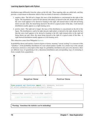
Fig. 1: Same Stats, Different Graphs
Histogram
Warning: Histograms are often confused with Bar graphs!
The fundamental difference between histogram and bar graph will help you to identify the two easily is that
there are gaps between bars in a bar graph but in the histogram, the bars are adjacent to each other. The
interested reader is referred to Difference Between Histogram and Bar Graph.
var = 'Age (years)'
x = data1[var]
bins = np.arange(0, 100, 5.0)
(continues on next page)
7.1. Univariate Analysis 71](https://image.slidesharecdn.com/pyspark-230429134708-b35c8a19/85/pyspark-pdf-77-320.jpg)
![Learning Apache Spark with Python
(continued from previous page)
plt.figure(figsize=(10,8))
# the histogram of the data
plt.hist(x, bins, alpha=0.8, histtype='bar', color='gold',
ec='black',weights=np.zeros_like(x) + 100. / x.size)
plt.xlabel(var)
plt.ylabel('percentage')
plt.xticks(bins)
plt.show()
fig.savefig(var+".pdf", bbox_inches='tight')
var = 'Age (years)'
x = data1[var]
bins = np.arange(0, 100, 5.0)
(continues on next page)
72 Chapter 7. Data Exploration](https://image.slidesharecdn.com/pyspark-230429134708-b35c8a19/85/pyspark-pdf-78-320.jpg)
![Learning Apache Spark with Python
(continued from previous page)
########################################################################
hist, bin_edges = np.histogram(x,bins,
weights=np.zeros_like(x) + 100. / x.size)
# make the histogram
fig = plt.figure(figsize=(20, 8))
ax = fig.add_subplot(1, 2, 1)
# Plot the histogram heights against integers on the x axis
ax.bar(range(len(hist)),hist,width=1,alpha=0.8,ec ='black', color='gold')
# # Set the ticks to the middle of the bars
ax.set_xticks([0.5+i for i,j in enumerate(hist)])
# Set the xticklabels to a string that tells us what the bin edges were
labels =['{}'.format(int(bins[i+1])) for i,j in enumerate(hist)]
labels.insert(0,'0')
ax.set_xticklabels(labels)
plt.xlabel(var)
plt.ylabel('percentage')
########################################################################
hist, bin_edges = np.histogram(x,bins) # make the histogram
ax = fig.add_subplot(1, 2, 2)
# Plot the histogram heights against integers on the x axis
ax.bar(range(len(hist)),hist,width=1,alpha=0.8,ec ='black', color='gold')
# # Set the ticks to the middle of the bars
ax.set_xticks([0.5+i for i,j in enumerate(hist)])
# Set the xticklabels to a string that tells us what the bin edges were
labels =['{}'.format(int(bins[i+1])) for i,j in enumerate(hist)]
labels.insert(0,'0')
ax.set_xticklabels(labels)
plt.xlabel(var)
plt.ylabel('count')
plt.suptitle('Histogram of {}: Left with percentage output;Right with count
˓
→output'
.format(var), size=16)
plt.show()
fig.savefig(var+".pdf", bbox_inches='tight')
7.1. Univariate Analysis 73](https://image.slidesharecdn.com/pyspark-230429134708-b35c8a19/85/pyspark-pdf-79-320.jpg)
![Learning Apache Spark with Python
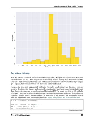
Sometimes, some people will ask you to plot the unequal width (invalid argument for histogram) of the bars.
You can still achieve it by the following trick.
var = 'Credit Amount'
plot_data = df.select(var).toPandas()
x= plot_data[var]
bins =[0,200,400,600,700,800,900,1000,2000,3000,4000,5000,6000,10000,25000]
hist, bin_edges = np.histogram(x,bins,weights=np.zeros_like(x) + 100. / x.
˓
→size) # make the histogram
fig = plt.figure(figsize=(10, 8))
ax = fig.add_subplot(1, 1, 1)
# Plot the histogram heights against integers on the x axis
ax.bar(range(len(hist)),hist,width=1,alpha=0.8,ec ='black',color = 'gold')
# # Set the ticks to the middle of the bars
ax.set_xticks([0.5+i for i,j in enumerate(hist)])
# Set the xticklabels to a string that tells us what the bin edges were
#labels =['{}k'.format(int(bins[i+1]/1000)) for i,j in enumerate(hist)]
labels =['{}'.format(bins[i+1]) for i,j in enumerate(hist)]
labels.insert(0,'0')
ax.set_xticklabels(labels)
#plt.text(-0.6, -1.4,'0')
plt.xlabel(var)
plt.ylabel('percentage')
plt.show()
74 Chapter 7. Data Exploration](https://image.slidesharecdn.com/pyspark-230429134708-b35c8a19/85/pyspark-pdf-80-320.jpg)
![Learning Apache Spark with Python
(continued from previous page)
ax = fig.add_subplot(1, 2, 2)
ax = sns.violinplot(data=x)
7.1.2 Categorical Variables
Compared with the numerical variables, the categorical variables are much more easier to do the exploration.
Frequency table
from pyspark.sql import functions as F
from pyspark.sql.functions import rank,sum,col
from pyspark.sql import Window
window = Window.rowsBetween(Window.unboundedPreceding,Window.
˓
→unboundedFollowing)
# withColumn('Percent %',F.format_string("%5.0f%%n",col('Credit_num')*100/
˓
→col('total'))).
tab = df.select(['age_class','Credit Amount']).
groupBy('age_class').
agg(F.count('Credit Amount').alias('Credit_num'),
F.mean('Credit Amount').alias('Credit_avg'),
F.min('Credit Amount').alias('Credit_min'),
F.max('Credit Amount').alias('Credit_max')).
withColumn('total',sum(col('Credit_num')).over(window)).
withColumn('Percent',col('Credit_num')*100/col('total')).
drop(col('total'))
+---------+----------+------------------+----------+----------+-------+
|age_class|Credit_num| Credit_avg|Credit_min|Credit_max|Percent|
+---------+----------+------------------+----------+----------+-------+
(continues on next page)
76 Chapter 7. Data Exploration](https://image.slidesharecdn.com/pyspark-230429134708-b35c8a19/85/pyspark-pdf-82-320.jpg)
![Learning Apache Spark with Python
(continued from previous page)
| 45-54| 120|3183.0666666666666| 338| 12612| 12.0|
| <25| 150| 2970.733333333333| 276| 15672| 15.0|
| 55-64| 56| 3493.660714285714| 385| 15945| 5.6|
| 35-44| 254| 3403.771653543307| 250| 15857| 25.4|
| 25-34| 397| 3298.823677581864| 343| 18424| 39.7|
| 65+| 23|3210.1739130434785| 571| 14896| 2.3|
+---------+----------+------------------+----------+----------+-------+
Pie plot
# Data to plot
labels = plot_data.age_class
sizes = plot_data.Percent
colors = ['gold', 'yellowgreen', 'lightcoral','blue', 'lightskyblue','green',
˓
→'red']
explode = (0, 0.1, 0, 0,0,0) # explode 1st slice
# Plot
plt.figure(figsize=(10,8))
plt.pie(sizes, explode=explode, labels=labels, colors=colors,
autopct='%1.1f%%', shadow=True, startangle=140)
plt.axis('equal')
plt.show()
7.1. Univariate Analysis 77](https://image.slidesharecdn.com/pyspark-230429134708-b35c8a19/85/pyspark-pdf-83-320.jpg)
![Learning Apache Spark with Python
Bar plot
labels = plot_data.age_class
missing = plot_data.Percent
ind = [x for x, _ in enumerate(labels)]
plt.figure(figsize=(10,8))
plt.bar(ind, missing, width=0.8, label='missing', color='gold')
plt.xticks(ind, labels)
plt.ylabel("percentage")
plt.show()
78 Chapter 7. Data Exploration](https://image.slidesharecdn.com/pyspark-230429134708-b35c8a19/85/pyspark-pdf-84-320.jpg)
![Learning Apache Spark with Python
labels = ['missing', '<25', '25-34', '35-44', '45-54','55-64','65+']
missing = np.array([0.000095, 0.024830, 0.028665, 0.029477, 0.031918,0.037073,
˓
→0.026699])
man = np.array([0.000147, 0.036311, 0.038684, 0.044761, 0.051269, 0.059542, 0.
˓
→054259])
women = np.array([0.004035, 0.032935, 0.035351, 0.041778, 0.048437, 0.056236,
˓
→0.048091])
ind = [x for x, _ in enumerate(labels)]
plt.figure(figsize=(10,8))
plt.bar(ind, women, width=0.8, label='women', color='gold',
˓
→bottom=man+missing)
plt.bar(ind, man, width=0.8, label='man', color='silver', bottom=missing)
plt.bar(ind, missing, width=0.8, label='missing', color='#CD853F')
plt.xticks(ind, labels)
plt.ylabel("percentage")
plt.legend(loc="upper left")
plt.title("demo")
plt.show()
7.1. Univariate Analysis 79](https://image.slidesharecdn.com/pyspark-230429134708-b35c8a19/85/pyspark-pdf-85-320.jpg)
![Learning Apache Spark with Python
7.2 Multivariate Analysis
In this section, I will only demostrate the bivariate analysis. Since the multivariate analysis is the generation
of the bivariate.
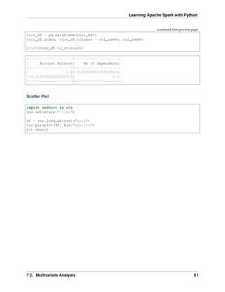
7.2.1 Numerical V.S. Numerical
Correlation matrix
from pyspark.mllib.stat import Statistics
import pandas as pd
corr_data = df.select(num_cols)
col_names = corr_data.columns
features = corr_data.rdd.map(lambda row: row[0:])
corr_mat=Statistics.corr(features, method="pearson")
(continues on next page)
80 Chapter 7. Data Exploration](https://image.slidesharecdn.com/pyspark-230429134708-b35c8a19/85/pyspark-pdf-86-320.jpg)
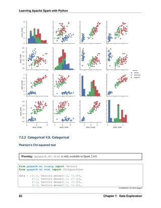
![Learning Apache Spark with Python
(continued from previous page)
(0.0, Vectors.dense(3.5, 40.0)),
(1.0, Vectors.dense(3.5, 40.0))]
df = spark.createDataFrame(data, ["label", "features"])
r = ChiSquareTest.test(df, "features", "label").head()
print("pValues: " + str(r.pValues))
print("degreesOfFreedom: " + str(r.degreesOfFreedom))
print("statistics: " + str(r.statistics))
pValues: [0.687289278791,0.682270330336]
degreesOfFreedom: [2, 3]
statistics: [0.75,1.5]
Cross table
df.stat.crosstab("age_class", "Occupation").show()
+--------------------+---+---+---+---+
|age_class_Occupation| 1| 2| 3| 4|
+--------------------+---+---+---+---+
| <25| 4| 34|108| 4|
| 55-64| 1| 15| 31| 9|
| 25-34| 7| 61|269| 60|
| 35-44| 4| 58|143| 49|
| 65+| 5| 3| 6| 9|
| 45-54| 1| 29| 73| 17|
+--------------------+---+---+---+---+
Stacked plot
labels = ['missing', '<25', '25-34', '35-44', '45-54','55-64','65+']
missing = np.array([0.000095, 0.024830, 0.028665, 0.029477, 0.031918,0.037073,
˓
→0.026699])
man = np.array([0.000147, 0.036311, 0.038684, 0.044761, 0.051269, 0.059542, 0.
˓
→054259])
women = np.array([0.004035, 0.032935, 0.035351, 0.041778, 0.048437, 0.056236,
˓
→0.048091])
ind = [x for x, _ in enumerate(labels)]
plt.figure(figsize=(10,8))
plt.bar(ind, women, width=0.8, label='women', color='gold',
˓
→bottom=man+missing)
plt.bar(ind, man, width=0.8, label='man', color='silver', bottom=missing)
plt.bar(ind, missing, width=0.8, label='missing', color='#CD853F')
plt.xticks(ind, labels)
plt.ylabel("percentage")
(continues on next page)
7.2. Multivariate Analysis 83](https://image.slidesharecdn.com/pyspark-230429134708-b35c8a19/85/pyspark-pdf-89-320.jpg)
![Learning Apache Spark with Python
(continued from previous page)
plt.legend(loc="upper left")
plt.title("demo")
plt.show()
7.2.3 Numerical V.S. Categorical
Line Chart with Error Bars
import pandas as pd
import numpy as np
import matplotlib.pyplot as plt
import seaborn as sns
from scipy import stats
%matplotlib inline
plt.rcParams['figure.figsize'] =(16,9)
plt.style.use('ggplot')
(continues on next page)
84 Chapter 7. Data Exploration](https://image.slidesharecdn.com/pyspark-230429134708-b35c8a19/85/pyspark-pdf-90-320.jpg)
![Learning Apache Spark with Python
(continued from previous page)
sns.set()
ax = sns.pointplot(x="day", y="tip", data=tips, capsize=.2)
plt.show()
Combination Chart
import pandas as pd
import numpy as np
import matplotlib.pyplot as plt
import seaborn as sns
from scipy import stats
%matplotlib inline
plt.rcParams['figure.figsize'] =(16,9)
plt.style.use('ggplot')
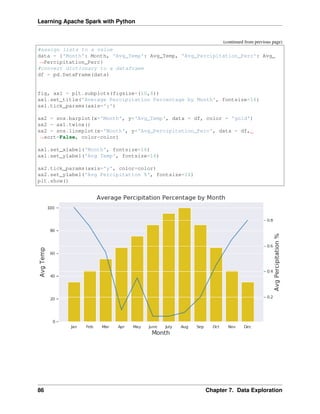
sns.set()
#create list of months
Month = ['Jan', 'Feb', 'Mar', 'Apr', 'May', 'June',
'July', 'Aug', 'Sep', 'Oct', 'Nov', 'Dec']
#create list for made up average temperatures
Avg_Temp = [35, 45, 55, 65, 75, 85, 95, 100, 85, 65, 45, 35]
#create list for made up average percipitation %
Avg_Percipitation_Perc = [.90, .75, .55, .10, .35, .05, .05, .08, .20, .45, .
˓
→65, .80]
(continues on next page)
7.2. Multivariate Analysis 85](https://image.slidesharecdn.com/pyspark-230429134708-b35c8a19/85/pyspark-pdf-91-320.jpg)
![Learning Apache Spark with Python
d. a source of the information loss - in case of HashingTF it is dimensionality reduction with possible
collisions. CountVectorizer discards infrequent tokens. How it affects downstream models depends
on a particular use case and data.
HashingTF and CountVectorizer are the two popular alogoritms which used to generate term frequency
vectors. They basically convert documents into a numerical representation which can be fed directly or with
further processing into other algorithms like LDA, MinHash for Jaccard Distance, Cosine Distance.
• 𝑡: term
• 𝑑: document
• 𝐷: corpus
• |𝐷|: the number of the elements in corpus
• 𝑇𝐹(𝑡, 𝑑): Term Frequency: the number of times that term 𝑡 appears in document 𝑑
• 𝐷𝐹(𝑡, 𝐷): Document Frequency: the number of documents that contains term 𝑡
• 𝐼𝐷𝐹(𝑡, 𝐷): Inverse Document Frequency is a numerical measure of how much information a term
provides
𝐼𝐷𝐹(𝑡, 𝐷) = log
|𝐷| + 1
𝐷𝐹(𝑡, 𝐷) + 1
• 𝑇𝐹𝐼𝐷𝐹(𝑡, 𝑑, 𝐷) the product of TF and IDF
𝑇𝐹𝐼𝐷𝐹(𝑡, 𝑑, 𝐷) = 𝑇𝐹(𝑡, 𝑑) · 𝐼𝐷𝐹(𝑡, 𝐷)
Let’s look at the example:
from pyspark.ml import Pipeline
from pyspark.ml.feature import HashingTF, IDF, Tokenizer
sentenceData = spark.createDataFrame([
(0, "Python python Spark Spark"),
(1, "Python SQL")],
["document", "sentence"])
sentenceData.show(truncate=False)
+--------+-------------------------+
|document|sentence |
+--------+-------------------------+
|0 |Python python Spark Spark|
|1 |Python SQL |
+--------+-------------------------+
Then:
• 𝑇𝐹(𝑝𝑦𝑡ℎ𝑜𝑛, 𝑑𝑜𝑐𝑢𝑚𝑒𝑛𝑡1) = 1, 𝑇𝐹(𝑠𝑝𝑎𝑟𝑘, 𝑑𝑜𝑐𝑢𝑚𝑒𝑛𝑡1) = 2
• 𝐷𝐹(𝑆𝑝𝑎𝑟𝑘, 𝐷) = 2, 𝐷𝐹(𝑠𝑞𝑙, 𝐷) = 1
• IDF:
88 Chapter 8. Data Manipulation: Features](https://image.slidesharecdn.com/pyspark-230429134708-b35c8a19/85/pyspark-pdf-94-320.jpg)
![Learning Apache Spark with Python
𝐼𝐷𝐹(𝑝𝑦𝑡ℎ𝑜𝑛, 𝐷) = log
|𝐷| + 1
𝐷𝐹(𝑡, 𝐷) + 1
= log(
2 + 1
2 + 1
) = 0
𝐼𝐷𝐹(𝑠𝑝𝑎𝑟𝑘, 𝐷) = log
|𝐷| + 1
𝐷𝐹(𝑡, 𝐷) + 1
= log(
2 + 1
1 + 1
) = 0.4054651081081644
𝐼𝐷𝐹(𝑠𝑞𝑙, 𝐷) = log
|𝐷| + 1
𝐷𝐹(𝑡, 𝐷) + 1
= log(
2 + 1
1 + 1
) = 0.4054651081081644
• TFIDF
𝑇𝐹𝐼𝐷𝐹(𝑝𝑦𝑡ℎ𝑜𝑛, 𝑑𝑜𝑐𝑢𝑚𝑒𝑛𝑡1, 𝐷) = 3 * 0 = 0
𝑇𝐹𝐼𝐷𝐹(𝑠𝑝𝑎𝑟𝑘, 𝑑𝑜𝑐𝑢𝑚𝑒𝑛𝑡1, 𝐷) = 2 * 0.4054651081081644 = 0.8109302162163288
𝑇𝐹𝐼𝐷𝐹(𝑠𝑞𝑙, 𝑑𝑜𝑐𝑢𝑚𝑒𝑛𝑡1, 𝐷) = 1 * 0.4054651081081644 = 0.4054651081081644
Countvectorizer
Stackoverflow TF: CountVectorizer and CountVectorizerModel aim to help convert a collection of text doc-
uments to vectors of token counts. When an a-priori dictionary is not available, CountVectorizer can be
used as an Estimator to extract the vocabulary, and generates a CountVectorizerModel. The model produces
sparse representations for the documents over the vocabulary, which can then be passed to other algorithms
like LDA.
from pyspark.ml import Pipeline
from pyspark.ml.feature import CountVectorizer
from pyspark.ml.feature import HashingTF, IDF, Tokenizer
sentenceData = spark.createDataFrame([
(0, "Python python Spark Spark"),
(1, "Python SQL")],
["document", "sentence"])
tokenizer = Tokenizer(inputCol="sentence", outputCol="words")
vectorizer = CountVectorizer(inputCol="words", outputCol="rawFeatures")
idf = IDF(inputCol="rawFeatures", outputCol="features")
pipeline = Pipeline(stages=[tokenizer, vectorizer, idf])
model = pipeline.fit(sentenceData)
import numpy as np
total_counts = model.transform(sentenceData)
.select('rawFeatures').rdd
.map(lambda row: row['rawFeatures'].toArray())
.reduce(lambda x,y: [x[i]+y[i] for i in range(len(y))])
vocabList = model.stages[1].vocabulary
d = {'vocabList':vocabList,'counts':total_counts}
(continues on next page)
8.1. Feature Extraction 89](https://image.slidesharecdn.com/pyspark-230429134708-b35c8a19/85/pyspark-pdf-95-320.jpg)
![Learning Apache Spark with Python
(continued from previous page)
spark.createDataFrame(np.array(list(d.values())).T.tolist(),list(d.keys())).
˓
→show()
counts = model.transform(sentenceData).select('rawFeatures').collect()
counts
[Row(rawFeatures=SparseVector(8, {0: 1.0, 1: 1.0, 2: 1.0})),
Row(rawFeatures=SparseVector(8, {0: 1.0, 1: 1.0, 4: 1.0})),
Row(rawFeatures=SparseVector(8, {0: 1.0, 3: 1.0, 5: 1.0, 6: 1.0, 7: 1.0}))]
+---------+------+
|vocabList|counts|
+---------+------+
| python| 3.0|
| spark| 2.0|
| sql| 1.0|
+---------+------+
model.transform(sentenceData).show(truncate=False)
+--------+-------------------------+------------------------------+-----------
˓
→--------+----------------------------------+
|document|sentence |words
˓
→|rawFeatures |features |
+--------+-------------------------+------------------------------+-----------
˓
→--------+----------------------------------+
|0 |Python python Spark Spark|[python, python, spark, spark]|(3,[0,1],
˓
→[2.0,2.0])|(3,[0,1],[0.0,0.8109302162163288])|
|1 |Python SQL |[python, sql] |(3,[0,2],
˓
→[1.0,1.0])|(3,[0,2],[0.0,0.4054651081081644])|
+--------+-------------------------+------------------------------+-----------
˓
→--------+----------------------------------+
from pyspark.sql.types import ArrayType, StringType
def termsIdx2Term(vocabulary):
def termsIdx2Term(termIndices):
return [vocabulary[int(index)] for index in termIndices]
return udf(termsIdx2Term, ArrayType(StringType()))
vectorizerModel = model.stages[1]
vocabList = vectorizerModel.vocabulary
vocabList
['python', 'spark', 'sql']
rawFeatures = model.transform(sentenceData).select('rawFeatures')
rawFeatures.show()
(continues on next page)
90 Chapter 8. Data Manipulation: Features](https://image.slidesharecdn.com/pyspark-230429134708-b35c8a19/85/pyspark-pdf-96-320.jpg)
![Learning Apache Spark with Python
(continued from previous page)
+-------------------+
| rawFeatures|
+-------------------+
|(3,[0,1],[2.0,2.0])|
|(3,[0,2],[1.0,1.0])|
+-------------------+
from pyspark.sql.functions import udf
import pyspark.sql.functions as F
from pyspark.sql.types import StringType, DoubleType, IntegerType
indices_udf = udf(lambda vector: vector.indices.tolist(),
˓
→ArrayType(IntegerType()))
values_udf = udf(lambda vector: vector.toArray().tolist(),
˓
→ArrayType(DoubleType()))
rawFeatures.withColumn('indices', indices_udf(F.col('rawFeatures')))
.withColumn('values', values_udf(F.col('rawFeatures')))
.withColumn("Terms", termsIdx2Term(vocabList)("indices")).show()
+-------------------+-------+---------------+---------------+
| rawFeatures|indices| values| Terms|
+-------------------+-------+---------------+---------------+
|(3,[0,1],[2.0,2.0])| [0, 1]|[2.0, 2.0, 0.0]|[python, spark]|
|(3,[0,2],[1.0,1.0])| [0, 2]|[1.0, 0.0, 1.0]| [python, sql]|
+-------------------+-------+---------------+---------------+
HashingTF
Stackoverflow TF: HashingTF is a Transformer which takes sets of terms and converts those sets into fixed-
length feature vectors. In text processing, a “set of terms” might be a bag of words. HashingTF utilizes
the hashing trick. A raw feature is mapped into an index (term) by applying a hash function. The hash
function used here is MurmurHash 3. Then term frequencies are calculated based on the mapped indices.
This approach avoids the need to compute a global term-to-index map, which can be expensive for a large
corpus, but it suffers from potential hash collisions, where different raw features may become the same term
after hashing.
from pyspark.ml import Pipeline
from pyspark.ml.feature import HashingTF, IDF, Tokenizer
sentenceData = spark.createDataFrame([
(0, "Python python Spark Spark"),
(1, "Python SQL")],
["document", "sentence"])
tokenizer = Tokenizer(inputCol="sentence", outputCol="words")
(continues on next page)
8.1. Feature Extraction 91](https://image.slidesharecdn.com/pyspark-230429134708-b35c8a19/85/pyspark-pdf-97-320.jpg)
![Learning Apache Spark with Python
(continued from previous page)
vectorizer = HashingTF(inputCol="words", outputCol="rawFeatures",
˓
→numFeatures=5)
idf = IDF(inputCol="rawFeatures", outputCol="features")
pipeline = Pipeline(stages=[tokenizer, vectorizer, idf])
model = pipeline.fit(sentenceData)
model.transform(sentenceData).show(truncate=False)
+--------+-------------------------+------------------------------+-----------
˓
→--------+----------------------------------+
|document|sentence |words
˓
→|rawFeatures |features |
+--------+-------------------------+------------------------------+-----------
˓
→--------+----------------------------------+
|0 |Python python Spark Spark|[python, python, spark, spark]|(5,[0,4],
˓
→[2.0,2.0])|(5,[0,4],[0.8109302162163288,0.0])|
|1 |Python SQL |[python, sql] |(5,[1,4],
˓
→[1.0,1.0])|(5,[1,4],[0.4054651081081644,0.0])|
+--------+-------------------------+------------------------------+-----------
˓
→--------+----------------------------------+
8.1.2 Word2Vec
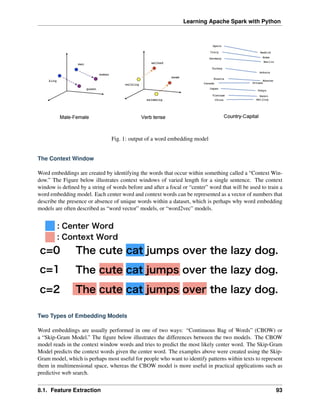
Word Embeddings
Word2Vec is one of the popupar method to implement the Word Embeddings. Word embeddings (The
best tutorial I have read. The following word and images content are from Chris Bail, PhD Duke University.
So the copyright belongs to Chris Bail, PhD Duke University.) gained fame in the world of automated text
analysis when it was demonstrated that they could be used to identify analogies. Figure 1 illustrates the
output of a word embedding model where individual words are plotted in three dimensional space generated
by the model. By examining the adjacency of words in this space, word embedding models can complete
analogies such as “Man is to woman as king is to queen.” If you’d like to explore what the output of a large
word embedding model looks like in more detail, check out this fantastic visualization of most words in the
English language that was produced using a word embedding model called GloVE.
92 Chapter 8. Data Manipulation: Features](https://image.slidesharecdn.com/pyspark-230429134708-b35c8a19/85/pyspark-pdf-98-320.jpg)
![Learning Apache Spark with Python
Word Embedding Models in PySpark
from pyspark.ml.feature import Word2Vec
from pyspark.ml import Pipeline
tokenizer = Tokenizer(inputCol="sentence", outputCol="words")
word2Vec = Word2Vec(vectorSize=3, minCount=0, inputCol="words", outputCol=
˓
→"feature")
pipeline = Pipeline(stages=[tokenizer, word2Vec])
model = pipeline.fit(sentenceData)
result = model.transform(sentenceData)
result.show()
+-----+--------------------+--------------------+--------------------+
|label| sentence| words| feature|
+-----+--------------------+--------------------+--------------------+
| 0.0| I love Spark| [i, love, spark]|[0.05594437588782...|
| 0.0| I love python| [i, love, python]|[-0.0350368790871...|
| 1.0|I think ML is awe...|[i, think, ml, is...|[0.01242086507845...|
+-----+--------------------+--------------------+--------------------+
w2v = model.stages[1]
w2v.getVectors().show()
(continues on next page)
94 Chapter 8. Data Manipulation: Features](https://image.slidesharecdn.com/pyspark-230429134708-b35c8a19/85/pyspark-pdf-100-320.jpg)
![Learning Apache Spark with Python
(continued from previous page)
+-------+-----------------------------------------------------------------+
|word |vector |
+-------+-----------------------------------------------------------------+
|is |[0.13657838106155396,0.060924094170331955,-0.03379475697875023] |
|awesome|[0.037024181336164474,-0.023855900391936302,0.0760037824511528] |
|i |[-0.0014482572441920638,0.049365971237421036,0.12016955763101578]|
|ml |[-0.14006119966506958,0.01626444421708584,0.042281970381736755] |
|spark |[0.1589149385690689,-0.10970081388950348,-0.10547549277544022] |
|think |[0.030011219903826714,-0.08994936943054199,0.16471518576145172] |
|love |[0.01036644633859396,-0.017782460898160934,0.08870164304971695] |
|python |[-0.11402882635593414,0.045119188725948334,-0.029877422377467155]|
+-------+-----------------------------------------------------------------+
from pyspark.sql.functions import format_number as fmt
w2v.findSynonyms("could", 2).select("word", fmt("similarity", 5).alias(
˓
→"similarity")).show()
+-------+----------+
| word|similarity|
+-------+----------+
|classes| 0.90232|
| i| 0.75424|
+-------+----------+
8.1.3 FeatureHasher
from pyspark.ml.feature import FeatureHasher
dataset = spark.createDataFrame([
(2.2, True, "1", "foo"),
(3.3, False, "2", "bar"),
(4.4, False, "3", "baz"),
(5.5, False, "4", "foo")
], ["real", "bool", "stringNum", "string"])
hasher = FeatureHasher(inputCols=["real", "bool", "stringNum", "string"],
outputCol="features")
featurized = hasher.transform(dataset)
featurized.show(truncate=False)
+----+-----+---------+------+-------------------------------------------------
˓
→-------+
|real|bool |stringNum|string|features
˓
→ |
+----+-----+---------+------+-------------------------------------------------
˓
→-------+
|2.2 |true |1 |foo |(262144,[174475,247670,257907,262126],[2.2,1.0,1.
˓
→0,1.0])| (continues on next page)
8.1. Feature Extraction 95](https://image.slidesharecdn.com/pyspark-230429134708-b35c8a19/85/pyspark-pdf-101-320.jpg)
![Learning Apache Spark with Python
(continued from previous page)
|3.3 |false|2 |bar |(262144,[70644,89673,173866,174475],[1.0,1.0,1.0,
˓
→3.3]) |
|4.4 |false|3 |baz |(262144,[22406,70644,174475,187923],[1.0,1.0,4.4,
˓
→1.0]) |
|5.5 |false|4 |foo |(262144,[70644,101499,174475,257907],[1.0,1.0,5.
˓
→5,1.0]) |
+----+-----+---------+------+-------------------------------------------------
˓
→-------+
8.1.4 RFormula
from pyspark.ml.feature import RFormula
dataset = spark.createDataFrame(
[(7, "US", 18, 1.0),
(8, "CA", 12, 0.0),
(9, "CA", 15, 0.0)],
["id", "country", "hour", "clicked"])
formula = RFormula(
formula="clicked ~ country + hour",
featuresCol="features",
labelCol="label")
output = formula.fit(dataset).transform(dataset)
output.select("features", "label").show()
+----------+-----+
| features|label|
+----------+-----+
|[0.0,18.0]| 1.0|
|[1.0,12.0]| 0.0|
|[1.0,15.0]| 0.0|
+----------+-----+
8.2 Feature Transform
8.2.1 Tokenizer
from pyspark.ml.feature import Tokenizer, RegexTokenizer
from pyspark.sql.functions import col, udf
from pyspark.sql.types import IntegerType
sentenceDataFrame = spark.createDataFrame([
(0, "Hi I heard about Spark"),
(1, "I wish Java could use case classes"),
(continues on next page)
96 Chapter 8. Data Manipulation: Features](https://image.slidesharecdn.com/pyspark-230429134708-b35c8a19/85/pyspark-pdf-102-320.jpg)
![Learning Apache Spark with Python
(continued from previous page)
(2, "Logistic,regression,models,are,neat")
], ["id", "sentence"])
tokenizer = Tokenizer(inputCol="sentence", outputCol="words")
regexTokenizer = RegexTokenizer(inputCol="sentence", outputCol="words",
˓
→pattern="W")
# alternatively, pattern="w+", gaps(False)
countTokens = udf(lambda words: len(words), IntegerType())
tokenized = tokenizer.transform(sentenceDataFrame)
tokenized.select("sentence", "words")
.withColumn("tokens", countTokens(col("words"))).show(truncate=False)
regexTokenized = regexTokenizer.transform(sentenceDataFrame)
regexTokenized.select("sentence", "words")
.withColumn("tokens", countTokens(col("words"))).show(truncate=False)
+-----------------------------------+-----------------------------------------
˓
→-+------+
|sentence |words
˓
→ |tokens|
+-----------------------------------+-----------------------------------------
˓
→-+------+
|Hi I heard about Spark |[hi, i, heard, about, spark]
˓
→ |5 |
|I wish Java could use case classes |[i, wish, java, could, use, case,
˓
→classes]|7 |
|Logistic,regression,models,are,neat|[logistic,regression,models,are,neat]
˓
→ |1 |
+-----------------------------------+-----------------------------------------
˓
→-+------+
+-----------------------------------+-----------------------------------------
˓
→-+------+
|sentence |words
˓
→ |tokens|
+-----------------------------------+-----------------------------------------
˓
→-+------+
|Hi I heard about Spark |[hi, i, heard, about, spark]
˓
→ |5 |
|I wish Java could use case classes |[i, wish, java, could, use, case,
˓
→classes]|7 |
|Logistic,regression,models,are,neat|[logistic, regression, models, are,
˓
→neat] |5 |
+-----------------------------------+-----------------------------------------
˓
→-+------+
8.2. Feature Transform 97](https://image.slidesharecdn.com/pyspark-230429134708-b35c8a19/85/pyspark-pdf-103-320.jpg)
![Learning Apache Spark with Python
8.2.2 StopWordsRemover
from pyspark.ml.feature import StopWordsRemover
sentenceData = spark.createDataFrame([
(0, ["I", "saw", "the", "red", "balloon"]),
(1, ["Mary", "had", "a", "little", "lamb"])
], ["id", "raw"])
remover = StopWordsRemover(inputCol="raw", outputCol="removeded")
remover.transform(sentenceData).show(truncate=False)
+---+----------------------------+--------------------+
|id |raw |removeded |
+---+----------------------------+--------------------+
|0 |[I, saw, the, red, balloon] |[saw, red, balloon] |
|1 |[Mary, had, a, little, lamb]|[Mary, little, lamb]|
+---+----------------------------+--------------------+
8.2.3 NGram
from pyspark.ml import Pipeline
from pyspark.ml.feature import CountVectorizer
from pyspark.ml.feature import HashingTF, IDF, Tokenizer
from pyspark.ml.feature import NGram
sentenceData = spark.createDataFrame([
(0.0, "I love Spark"),
(0.0, "I love python"),
(1.0, "I think ML is awesome")],
["label", "sentence"])
tokenizer = Tokenizer(inputCol="sentence", outputCol="words")
ngram = NGram(n=2, inputCol="words", outputCol="ngrams")
idf = IDF(inputCol="rawFeatures", outputCol="features")
pipeline = Pipeline(stages=[tokenizer, ngram])
model = pipeline.fit(sentenceData)
model.transform(sentenceData).show(truncate=False)
+-----+---------------------+---------------------------+---------------------
˓
→-----------------+
|label|sentence |words |ngrams
˓
→ |
+-----+---------------------+---------------------------+---------------------
˓
→-----------------+
(continues on next page)
98 Chapter 8. Data Manipulation: Features](https://image.slidesharecdn.com/pyspark-230429134708-b35c8a19/85/pyspark-pdf-104-320.jpg)
![Learning Apache Spark with Python
(continued from previous page)
|0.0 |I love Spark |[i, love, spark] |[i love, love spark]
˓
→ |
|0.0 |I love python |[i, love, python] |[i love, love
˓
→python] |
|1.0 |I think ML is awesome|[i, think, ml, is, awesome]|[i think, think ml,
˓
→ml is, is awesome]|
+-----+---------------------+---------------------------+---------------------
˓
→-----------------+
8.2.4 Binarizer
from pyspark.ml.feature import Binarizer
continuousDataFrame = spark.createDataFrame([
(0, 0.1),
(1, 0.8),
(2, 0.2),
(3,0.5)
], ["id", "feature"])
binarizer = Binarizer(threshold=0.5, inputCol="feature", outputCol="binarized_
˓
→feature")
binarizedDataFrame = binarizer.transform(continuousDataFrame)
print("Binarizer output with Threshold = %f" % binarizer.getThreshold())
binarizedDataFrame.show()
Binarizer output with Threshold = 0.500000
+---+-------+-----------------+
| id|feature|binarized_feature|
+---+-------+-----------------+
| 0| 0.1| 0.0|
| 1| 0.8| 1.0|
| 2| 0.2| 0.0|
| 3| 0.5| 0.0|
+---+-------+-----------------+
8.2.5 Bucketizer
[Bucketizer](https://spark.apache.org/docs/latest/ml-features.html#bucketizer) transforms a column of con-
tinuous features to a column of feature buckets, where the buckets are specified by users.
from pyspark.ml.feature import QuantileDiscretizer, Bucketizer
data = [(0, 18.0), (1, 19.0), (2, 8.0), (3, 5.0), (4, 2.0)]
df = spark.createDataFrame(data, ["id", "age"])
(continues on next page)
8.2. Feature Transform 99](https://image.slidesharecdn.com/pyspark-230429134708-b35c8a19/85/pyspark-pdf-105-320.jpg)
![Learning Apache Spark with Python
(continued from previous page)
print(df.show())
splits = [-float("inf"),3, 10,float("inf")]
result_bucketizer = Bucketizer(splits=splits, inputCol="age",outputCol="result
˓
→").transform(df)
result_bucketizer.show()
+---+----+
| id| age|
+---+----+
| 0|18.0|
| 1|19.0|
| 2| 8.0|
| 3| 5.0|
| 4| 2.0|
+---+----+
None
+---+----+------+
| id| age|result|
+---+----+------+
| 0|18.0| 2.0|
| 1|19.0| 2.0|
| 2| 8.0| 1.0|
| 3| 5.0| 1.0|
| 4| 2.0| 0.0|
+---+----+------+
8.2.6 QuantileDiscretizer
QuantileDiscretizer takes a column with continuous features and outputs a column with binned categorical
features. The number of bins is set by the numBuckets parameter. It is possible that the number of buckets
used will be smaller than this value, for example, if there are too few distinct values of the input to create
enough distinct quantiles.
from pyspark.ml.feature import QuantileDiscretizer, Bucketizer
data = [(0, 18.0), (1, 19.0), (2, 8.0), (3, 5.0), (4, 2.0)]
df = spark.createDataFrame(data, ["id", "age"])
print(df.show())
qds = QuantileDiscretizer(numBuckets=5, inputCol="age", outputCol="buckets",
relativeError=0.01, handleInvalid="error")
bucketizer = qds.fit(df)
bucketizer.transform(df).show()
bucketizer.setHandleInvalid("skip").transform(df).show()
+---+----+
| id| age|
(continues on next page)
100 Chapter 8. Data Manipulation: Features](https://image.slidesharecdn.com/pyspark-230429134708-b35c8a19/85/pyspark-pdf-106-320.jpg)
![Learning Apache Spark with Python
(continued from previous page)
+---+----+
| 0|18.0|
| 1|19.0|
| 2| 8.0|
| 3| 5.0|
| 4| 2.0|
+---+----+
None
+---+----+-------+
| id| age|buckets|
+---+----+-------+
| 0|18.0| 3.0|
| 1|19.0| 3.0|
| 2| 8.0| 2.0|
| 3| 5.0| 2.0|
| 4| 2.0| 1.0|
+---+----+-------+
+---+----+-------+
| id| age|buckets|
+---+----+-------+
| 0|18.0| 3.0|
| 1|19.0| 3.0|
| 2| 8.0| 2.0|
| 3| 5.0| 2.0|
| 4| 2.0| 1.0|
+---+----+-------+
If the data has NULL values, then you will get the following results:
from pyspark.ml.feature import QuantileDiscretizer, Bucketizer
data = [(0, 18.0), (1, 19.0), (2, 8.0), (3, 5.0), (4, None)]
df = spark.createDataFrame(data, ["id", "age"])
print(df.show())
splits = [-float("inf"),3, 10,float("inf")]
result_bucketizer = Bucketizer(splits=splits,
inputCol="age",outputCol="result").
˓
→transform(df)
result_bucketizer.show()
qds = QuantileDiscretizer(numBuckets=5, inputCol="age", outputCol="buckets",
relativeError=0.01, handleInvalid="error")
bucketizer = qds.fit(df)
bucketizer.transform(df).show()
bucketizer.setHandleInvalid("skip").transform(df).show()
+---+----+
| id| age|
(continues on next page)
8.2. Feature Transform 101](https://image.slidesharecdn.com/pyspark-230429134708-b35c8a19/85/pyspark-pdf-107-320.jpg)
![Learning Apache Spark with Python
(continued from previous page)
+---+----+
| 0|18.0|
| 1|19.0|
| 2| 8.0|
| 3| 5.0|
| 4|null|
+---+----+
None
+---+----+------+
| id| age|result|
+---+----+------+
| 0|18.0| 2.0|
| 1|19.0| 2.0|
| 2| 8.0| 1.0|
| 3| 5.0| 1.0|
| 4|null| null|
+---+----+------+
+---+----+-------+
| id| age|buckets|
+---+----+-------+
| 0|18.0| 3.0|
| 1|19.0| 4.0|
| 2| 8.0| 2.0|
| 3| 5.0| 1.0|
| 4|null| null|
+---+----+-------+
+---+----+-------+
| id| age|buckets|
+---+----+-------+
| 0|18.0| 3.0|
| 1|19.0| 4.0|
| 2| 8.0| 2.0|
| 3| 5.0| 1.0|
+---+----+-------+
8.2.7 StringIndexer
from pyspark.ml.feature import StringIndexer
df = spark.createDataFrame(
[(0, "a"), (1, "b"), (2, "c"), (3, "a"), (4, "a"), (5, "c")],
["id", "category"])
indexer = StringIndexer(inputCol="category", outputCol="categoryIndex")
indexed = indexer.fit(df).transform(df)
indexed.show()
102 Chapter 8. Data Manipulation: Features](https://image.slidesharecdn.com/pyspark-230429134708-b35c8a19/85/pyspark-pdf-108-320.jpg)
![Learning Apache Spark with Python
+---+--------+-------------+
| id|category|categoryIndex|
+---+--------+-------------+
| 0| a| 0.0|
| 1| b| 2.0|
| 2| c| 1.0|
| 3| a| 0.0|
| 4| a| 0.0|
| 5| c| 1.0|
+---+--------+-------------+
8.2.8 labelConverter
from pyspark.ml.feature import IndexToString, StringIndexer
df = spark.createDataFrame(
[(0, "Yes"), (1, "Yes"), (2, "Yes"), (3, "No"), (4, "No"), (5, "No")],
["id", "label"])
indexer = StringIndexer(inputCol="label", outputCol="labelIndex")
model = indexer.fit(df)
indexed = model.transform(df)
print("Transformed string column '%s' to indexed column '%s'"
% (indexer.getInputCol(), indexer.getOutputCol()))
indexed.show()
print("StringIndexer will store labels in output column metadatan")
converter = IndexToString(inputCol="labelIndex", outputCol="originalLabel")
converted = converter.transform(indexed)
print("Transformed indexed column '%s' back to original string column '%s'
˓
→using "
"labels in metadata" % (converter.getInputCol(), converter.
˓
→getOutputCol()))
converted.select("id", "labelIndex", "originalLabel").show()
Transformed string column 'label' to indexed column 'labelIndex'
+---+-----+----------+
| id|label|labelIndex|
+---+-----+----------+
| 0| Yes| 1.0|
| 1| Yes| 1.0|
| 2| Yes| 1.0|
| 3| No| 0.0|
| 4| No| 0.0|
| 5| No| 0.0|
+---+-----+----------+
(continues on next page)
8.2. Feature Transform 103](https://image.slidesharecdn.com/pyspark-230429134708-b35c8a19/85/pyspark-pdf-109-320.jpg)
![Learning Apache Spark with Python
(continued from previous page)
StringIndexer will store labels in output column metadata
Transformed indexed column 'labelIndex' back to original string column
˓
→'originalLabel' using labels in metadata
+---+----------+-------------+
| id|labelIndex|originalLabel|
+---+----------+-------------+
| 0| 1.0| Yes|
| 1| 1.0| Yes|
| 2| 1.0| Yes|
| 3| 0.0| No|
| 4| 0.0| No|
| 5| 0.0| No|
+---+----------+-------------+
from pyspark.ml import Pipeline
from pyspark.ml.feature import IndexToString, StringIndexer
df = spark.createDataFrame(
[(0, "Yes"), (1, "Yes"), (2, "Yes"), (3, "No"), (4, "No"), (5, "No")],
["id", "label"])
indexer = StringIndexer(inputCol="label", outputCol="labelIndex")
converter = IndexToString(inputCol="labelIndex", outputCol="originalLabel")
pipeline = Pipeline(stages=[indexer, converter])
model = pipeline.fit(df)
result = model.transform(df)
result.show()
+---+-----+----------+-------------+
| id|label|labelIndex|originalLabel|
+---+-----+----------+-------------+
| 0| Yes| 1.0| Yes|
| 1| Yes| 1.0| Yes|
| 2| Yes| 1.0| Yes|
| 3| No| 0.0| No|
| 4| No| 0.0| No|
| 5| No| 0.0| No|
+---+-----+----------+-------------+
104 Chapter 8. Data Manipulation: Features](https://image.slidesharecdn.com/pyspark-230429134708-b35c8a19/85/pyspark-pdf-110-320.jpg)
![Learning Apache Spark with Python
8.2.9 VectorIndexer
from pyspark.ml import Pipeline
from pyspark.ml.regression import LinearRegression
from pyspark.ml.feature import VectorIndexer
from pyspark.ml.evaluation import RegressionEvaluator
from pyspark.ml.feature import RFormula
df = spark.createDataFrame([
(0, 2.2, True, "1", "foo", 'CA'),
(1, 3.3, False, "2", "bar", 'US'),
(0, 4.4, False, "3", "baz", 'CHN'),
(1, 5.5, False, "4", "foo", 'AUS')
], ['label',"real", "bool", "stringNum", "string","country"])
formula = RFormula(
formula="label ~ real + bool + stringNum + string + country",
featuresCol="features",
labelCol="label")
# Automatically identify categorical features, and index them.
# We specify maxCategories so features with > 4 distinct values
# are treated as continuous.
featureIndexer = VectorIndexer(inputCol="features",
outputCol="indexedFeatures",
maxCategories=2)
pipeline = Pipeline(stages=[formula, featureIndexer])
model = pipeline.fit(df)
result = model.transform(df)
result.show()
+-----+----+-----+---------+------+-------+--------------------+--------------
˓
→------+
|label|real| bool|stringNum|string|country| features|
˓
→indexedFeatures|
+-----+----+-----+---------+------+-------+--------------------+--------------
˓
→------+
| 0| 2.2| true| 1| foo| CA|(10,[0,1,5,7],[2....|(10,[0,1,5,7],
˓
→[2....|
| 1| 3.3|false| 2| bar| US|(10,[0,3,8],[3.3,...|(10,[0,3,8],
˓
→[3.3,...|
| 0| 4.4|false| 3| baz| CHN|(10,[0,4,6,9],[4....|(10,[0,4,6,9],
˓
→[4....|
| 1| 5.5|false| 4| foo| AUS|(10,[0,2,5],[5.5,...|(10,[0,2,5],
˓
→[5.5,...|
+-----+----+-----+---------+------+-------+--------------------+--------------
˓
→------+
8.2. Feature Transform 105](https://image.slidesharecdn.com/pyspark-230429134708-b35c8a19/85/pyspark-pdf-111-320.jpg)
![Learning Apache Spark with Python
8.2.10 VectorAssembler
from pyspark.ml.linalg import Vectors
from pyspark.ml.feature import VectorAssembler
dataset = spark.createDataFrame(
[(0, 18, 1.0, Vectors.dense([0.0, 10.0, 0.5]), 1.0)],
["id", "hour", "mobile", "userFeatures", "clicked"])
assembler = VectorAssembler(
inputCols=["hour", "mobile", "userFeatures"],
outputCol="features")
output = assembler.transform(dataset)
print("Assembled columns 'hour', 'mobile', 'userFeatures' to vector column
˓
→'features'")
output.select("features", "clicked").show(truncate=False)
Assembled columns 'hour', 'mobile', 'userFeatures' to vector column 'features'
+-----------------------+-------+
|features |clicked|
+-----------------------+-------+
|[18.0,1.0,0.0,10.0,0.5]|1.0 |
+-----------------------+-------+
8.2.11 OneHotEncoder
This is the note I wrote for one of my readers for explaining the OneHotEncoder. I would like to share it at
here:
Import and creating SparkSession
from pyspark.sql import SparkSession
spark = SparkSession
.builder
.appName("Python Spark create RDD example")
.config("spark.some.config.option", "some-value")
.getOrCreate()
df = spark.createDataFrame([
(0, "a"),
(1, "b"),
(2, "c"),
(3, "a"),
(4, "a"),
(5, "c")
], ["id", "category"])
df.show()
106 Chapter 8. Data Manipulation: Features](https://image.slidesharecdn.com/pyspark-230429134708-b35c8a19/85/pyspark-pdf-112-320.jpg)
![Learning Apache Spark with Python
+---+--------+
| id|category|
+---+--------+
| 0| a|
| 1| b|
| 2| c|
| 3| a|
| 4| a|
| 5| c|
+---+--------+
OneHotEncoder
Encoder
from pyspark.ml.feature import OneHotEncoder, StringIndexer
stringIndexer = StringIndexer(inputCol="category", outputCol="categoryIndex")
model = stringIndexer.fit(df)
indexed = model.transform(df)
# default setting: dropLast=True
encoder = OneHotEncoder(inputCol="categoryIndex", outputCol="categoryVec",
˓
→dropLast=False)
encoded = encoder.transform(indexed)
encoded.show()
+---+--------+-------------+-------------+
| id|category|categoryIndex| categoryVec|
+---+--------+-------------+-------------+
| 0| a| 0.0|(3,[0],[1.0])|
| 1| b| 2.0|(3,[2],[1.0])|
| 2| c| 1.0|(3,[1],[1.0])|
| 3| a| 0.0|(3,[0],[1.0])|
| 4| a| 0.0|(3,[0],[1.0])|
| 5| c| 1.0|(3,[1],[1.0])|
+---+--------+-------------+-------------+
Note: The default setting of OneHotEncoder is: dropLast=True
# default setting: dropLast=True
encoder = OneHotEncoder(inputCol="categoryIndex", outputCol=
˓
→"categoryVec")
encoded = encoder.transform(indexed)
encoded.show()
8.2. Feature Transform 107](https://image.slidesharecdn.com/pyspark-230429134708-b35c8a19/85/pyspark-pdf-113-320.jpg)
![Learning Apache Spark with Python
+---+--------+-------------+-------------+
| id|category|categoryIndex| categoryVec|
+---+--------+-------------+-------------+
| 0| a| 0.0|(2,[0],[1.0])|
| 1| b| 2.0| (2,[],[])|
| 2| c| 1.0|(2,[1],[1.0])|
| 3| a| 0.0|(2,[0],[1.0])|
| 4| a| 0.0|(2,[0],[1.0])|
| 5| c| 1.0|(2,[1],[1.0])|
+---+--------+-------------+-------------+
Vector Assembler
from pyspark.ml import Pipeline
from pyspark.ml.feature import VectorAssembler
categoricalCols = ['category']
indexers = [ StringIndexer(inputCol=c, outputCol="{0}_indexed".format(c))
for c in categoricalCols ]
# default setting: dropLast=True
encoders = [ OneHotEncoder(inputCol=indexer.getOutputCol(),
outputCol="{0}_encoded".format(indexer.getOutputCol()),
˓
→dropLast=False)
for indexer in indexers ]
assembler = VectorAssembler(inputCols=[encoder.getOutputCol() for encoder in
˓
→encoders]
, outputCol="features")
pipeline = Pipeline(stages=indexers + encoders + [assembler])
model=pipeline.fit(df)
data = model.transform(df)
data.show()
+---+--------+----------------+------------------------+-------------+
| id|category|category_indexed|category_indexed_encoded| features|
+---+--------+----------------+------------------------+-------------+
| 0| a| 0.0| (3,[0],[1.0])|[1.0,0.0,0.0]|
| 1| b| 2.0| (3,[2],[1.0])|[0.0,0.0,1.0]|
| 2| c| 1.0| (3,[1],[1.0])|[0.0,1.0,0.0]|
| 3| a| 0.0| (3,[0],[1.0])|[1.0,0.0,0.0]|
| 4| a| 0.0| (3,[0],[1.0])|[1.0,0.0,0.0]|
| 5| c| 1.0| (3,[1],[1.0])|[0.0,1.0,0.0]|
+---+--------+----------------+------------------------+-------------+
108 Chapter 8. Data Manipulation: Features](https://image.slidesharecdn.com/pyspark-230429134708-b35c8a19/85/pyspark-pdf-114-320.jpg)
![Learning Apache Spark with Python
Application: Get Dummy Variable
def get_dummy(df,indexCol,categoricalCols,continuousCols,labelCol,
˓
→dropLast=False):
'''
Get dummy variables and concat with continuous variables for ml modeling.
:param df: the dataframe
:param categoricalCols: the name list of the categorical data
:param continuousCols: the name list of the numerical data
:param labelCol: the name of label column
:param dropLast: the flag of drop last column
:return: feature matrix
:author: Wenqiang Feng
:email: von198@gmail.com
>>> df = spark.createDataFrame([
(0, "a"),
(1, "b"),
(2, "c"),
(3, "a"),
(4, "a"),
(5, "c")
], ["id", "category"])
>>> indexCol = 'id'
>>> categoricalCols = ['category']
>>> continuousCols = []
>>> labelCol = []
>>> mat = get_dummy(df,indexCol,categoricalCols,continuousCols,labelCol)
>>> mat.show()
>>>
+---+-------------+
| id| features|
+---+-------------+
| 0|[1.0,0.0,0.0]|
| 1|[0.0,0.0,1.0]|
| 2|[0.0,1.0,0.0]|
| 3|[1.0,0.0,0.0]|
| 4|[1.0,0.0,0.0]|
| 5|[0.0,1.0,0.0]|
+---+-------------+
'''
from pyspark.ml import Pipeline
from pyspark.ml.feature import StringIndexer, OneHotEncoder,
˓
→VectorAssembler
from pyspark.sql.functions import col
(continues on next page)
8.2. Feature Transform 109](https://image.slidesharecdn.com/pyspark-230429134708-b35c8a19/85/pyspark-pdf-115-320.jpg)
![Learning Apache Spark with Python
(continued from previous page)
indexers = [ StringIndexer(inputCol=c, outputCol="{0}_indexed".format(c))
for c in categoricalCols ]
# default setting: dropLast=True
encoders = [ OneHotEncoder(inputCol=indexer.getOutputCol(),
outputCol="{0}_encoded".format(indexer.getOutputCol()),
˓
→dropLast=dropLast)
for indexer in indexers ]
assembler = VectorAssembler(inputCols=[encoder.getOutputCol() for encoder
˓
→in encoders]
+ continuousCols, outputCol="features")
pipeline = Pipeline(stages=indexers + encoders + [assembler])
model=pipeline.fit(df)
data = model.transform(df)
if indexCol and labelCol:
# for supervised learning
data = data.withColumn('label',col(labelCol))
return data.select(indexCol,'features','label')
elif not indexCol and labelCol:
# for supervised learning
data = data.withColumn('label',col(labelCol))
return data.select('features','label')
elif indexCol and not labelCol:
# for unsupervised learning
return data.select(indexCol,'features')
elif not indexCol and not labelCol:
# for unsupervised learning
return data.select('features')
Unsupervised scenario
df = spark.createDataFrame([
(0, "a"),
(1, "b"),
(2, "c"),
(3, "a"),
(4, "a"),
(5, "c")
], ["id", "category"])
df.show()
indexCol = 'id'
categoricalCols = ['category']
continuousCols = []
labelCol = []
(continues on next page)
110 Chapter 8. Data Manipulation: Features](https://image.slidesharecdn.com/pyspark-230429134708-b35c8a19/85/pyspark-pdf-116-320.jpg)
![Learning Apache Spark with Python
(continued from previous page)
mat = get_dummy(df,indexCol,categoricalCols,continuousCols,labelCol)
mat.show()
+---+-------------+
| id| features|
+---+-------------+
| 0|[1.0,0.0,0.0]|
| 1|[0.0,0.0,1.0]|
| 2|[0.0,1.0,0.0]|
| 3|[1.0,0.0,0.0]|
| 4|[1.0,0.0,0.0]|
| 5|[0.0,1.0,0.0]|
+---+-------------+
Supervised scenario
df = spark.read.csv(path='bank.csv',
sep=',',encoding='UTF-8',comment=None,
header=True,inferSchema=True)
indexCol = []
catCols = ['job','marital','education','default',
'housing','loan','contact','poutcome']
contCols = ['balance', 'duration','campaign','pdays','previous']
labelCol = 'y'
data = get_dummy(df,indexCol,catCols,contCols,labelCol,dropLast=False)
data.show(5)
+--------------------+-----+
| features|label|
+--------------------+-----+
|(37,[8,12,17,19,2...| no|
|(37,[4,12,15,19,2...| no|
|(37,[0,13,16,19,2...| no|
|(37,[0,12,16,19,2...| no|
|(37,[1,12,15,19,2...| no|
+--------------------+-----+
only showing top 5 rows
The Jupyter Notebook can be found on Colab: OneHotEncoder .
8.2. Feature Transform 111](https://image.slidesharecdn.com/pyspark-230429134708-b35c8a19/85/pyspark-pdf-117-320.jpg)
![Learning Apache Spark with Python
8.2.12 Scaler
from pyspark.ml.feature import Normalizer, StandardScaler, MinMaxScaler,
˓
→MaxAbsScaler
scaler_type = 'Normal'
if scaler_type=='Normal':
scaler = Normalizer(inputCol="features", outputCol="scaledFeatures", p=1.
˓
→0)
elif scaler_type=='Standard':
scaler = StandardScaler(inputCol="features", outputCol="scaledFeatures",
withStd=True, withMean=False)
elif scaler_type=='MinMaxScaler':
scaler = MinMaxScaler(inputCol="features", outputCol="scaledFeatures")
elif scaler_type=='MaxAbsScaler':
scaler = MaxAbsScaler(inputCol="features", outputCol="scaledFeatures")
from pyspark.ml import Pipeline
from pyspark.ml.linalg import Vectors
df = spark.createDataFrame([
(0, Vectors.dense([1.0, 0.5, -1.0]),),
(1, Vectors.dense([2.0, 1.0, 1.0]),),
(2, Vectors.dense([4.0, 10.0, 2.0]),)
], ["id", "features"])
df.show()
pipeline = Pipeline(stages=[scaler])
model =pipeline.fit(df)
data = model.transform(df)
data.show()
+---+--------------+
| id| features|
+---+--------------+
| 0|[1.0,0.5,-1.0]|
| 1| [2.0,1.0,1.0]|
| 2|[4.0,10.0,2.0]|
+---+--------------+
+---+--------------+------------------+
| id| features| scaledFeatures|
+---+--------------+------------------+
| 0|[1.0,0.5,-1.0]| [0.4,0.2,-0.4]|
| 1| [2.0,1.0,1.0]| [0.5,0.25,0.25]|
| 2|[4.0,10.0,2.0]|[0.25,0.625,0.125]|
+---+--------------+------------------+
112 Chapter 8. Data Manipulation: Features](https://image.slidesharecdn.com/pyspark-230429134708-b35c8a19/85/pyspark-pdf-118-320.jpg)
![Learning Apache Spark with Python
Normalizer
from pyspark.ml.feature import Normalizer
from pyspark.ml.linalg import Vectors
dataFrame = spark.createDataFrame([
(0, Vectors.dense([1.0, 0.5, -1.0]),),
(1, Vectors.dense([2.0, 1.0, 1.0]),),
(2, Vectors.dense([4.0, 10.0, 2.0]),)
], ["id", "features"])
# Normalize each Vector using $L^1$ norm.
normalizer = Normalizer(inputCol="features", outputCol="normFeatures", p=1.0)
l1NormData = normalizer.transform(dataFrame)
print("Normalized using L^1 norm")
l1NormData.show()
# Normalize each Vector using $L^infty$ norm.
lInfNormData = normalizer.transform(dataFrame, {normalizer.p: float("inf")})
print("Normalized using L^inf norm")
lInfNormData.show()
Normalized using L^1 norm
+---+--------------+------------------+
| id| features| normFeatures|
+---+--------------+------------------+
| 0|[1.0,0.5,-1.0]| [0.4,0.2,-0.4]|
| 1| [2.0,1.0,1.0]| [0.5,0.25,0.25]|
| 2|[4.0,10.0,2.0]|[0.25,0.625,0.125]|
+---+--------------+------------------+
Normalized using L^inf norm
+---+--------------+--------------+
| id| features| normFeatures|
+---+--------------+--------------+
| 0|[1.0,0.5,-1.0]|[1.0,0.5,-1.0]|
| 1| [2.0,1.0,1.0]| [1.0,0.5,0.5]|
| 2|[4.0,10.0,2.0]| [0.4,1.0,0.2]|
+---+--------------+--------------+
StandardScaler
from pyspark.ml.feature import Normalizer, StandardScaler, MinMaxScaler,
˓
→MaxAbsScaler
from pyspark.ml.linalg import Vectors
dataFrame = spark.createDataFrame([
(0, Vectors.dense([1.0, 0.5, -1.0]),),
(1, Vectors.dense([2.0, 1.0, 1.0]),),
(continues on next page)
8.2. Feature Transform 113](https://image.slidesharecdn.com/pyspark-230429134708-b35c8a19/85/pyspark-pdf-119-320.jpg)
![Learning Apache Spark with Python
(continued from previous page)
(2, Vectors.dense([4.0, 10.0, 2.0]),)
], ["id", "features"])
scaler = StandardScaler(inputCol="features", outputCol="scaledFeatures",
withStd=True, withMean=False)
scaleredData = scaler.fit((dataFrame)).transform(dataFrame)
scaleredData.show(truncate=False)
+---+--------------+----------------------------------------------------------
˓
→--+
|id |features |scaledFeatures
˓
→ |
+---+--------------+----------------------------------------------------------
˓
→--+
|0 |[1.0,0.5,-1.0]|[0.6546536707079772,0.09352195295828244,-0.
˓
→6546536707079771]|
|1 |[2.0,1.0,1.0] |[1.3093073414159544,0.1870439059165649,0.
˓
→6546536707079771] |
|2 |[4.0,10.0,2.0]|[2.618614682831909,1.870439059165649,1.3093073414159542]
˓
→ |
+---+--------------+----------------------------------------------------------
˓
→--+
MinMaxScaler
from pyspark.ml.feature import Normalizer, StandardScaler, MinMaxScaler,
˓
→MaxAbsScaler
from pyspark.ml.linalg import Vectors
dataFrame = spark.createDataFrame([
(0, Vectors.dense([1.0, 0.5, -1.0]),),
(1, Vectors.dense([2.0, 1.0, 1.0]),),
(2, Vectors.dense([4.0, 10.0, 2.0]),)
], ["id", "features"])
scaler = MinMaxScaler(inputCol="features", outputCol="scaledFeatures")
scaledData = scaler.fit((dataFrame)).transform(dataFrame)
scaledData.show(truncate=False)
+---+--------------+----------------------------------------------------------
˓
→-+
|id |features |scaledFeatures
˓
→ |
+---+--------------+----------------------------------------------------------
˓
→-+
|0 |[1.0,0.5,-1.0]|[0.0,0.0,0.0]
˓
→ |
|1 |[2.0,1.0,1.0] |[0.3333333333333333,0.05263157894736842,0.
˓
→6666666666666666]| (continues on next page)
114 Chapter 8. Data Manipulation: Features](https://image.slidesharecdn.com/pyspark-230429134708-b35c8a19/85/pyspark-pdf-120-320.jpg)
![Learning Apache Spark with Python
(continued from previous page)
|2 |[4.0,10.0,2.0]|[1.0,1.0,1.0]
˓
→ |
+---+--------------+----------------------------------------------------------
˓
→-+
MaxAbsScaler
from pyspark.ml.feature import Normalizer, StandardScaler, MinMaxScaler,
˓
→MaxAbsScaler
from pyspark.ml.linalg import Vectors
dataFrame = spark.createDataFrame([
(0, Vectors.dense([1.0, 0.5, -1.0]),),
(1, Vectors.dense([2.0, 1.0, 1.0]),),
(2, Vectors.dense([4.0, 10.0, 2.0]),)
], ["id", "features"])
scaler = MaxAbsScaler(inputCol="features", outputCol="scaledFeatures")
scaledData = scaler.fit((dataFrame)).transform(dataFrame)
scaledData.show(truncate=False)
+---+--------------+----------------+
|id |features |scaledFeatures |
+---+--------------+----------------+
|0 |[1.0,0.5,-1.0]|[0.25,0.05,-0.5]|
|1 |[2.0,1.0,1.0] |[0.5,0.1,0.5] |
|2 |[4.0,10.0,2.0]|[1.0,1.0,1.0] |
+---+--------------+----------------+
8.2.13 PCA
from pyspark.ml.feature import PCA
from pyspark.ml.linalg import Vectors
data = [(Vectors.sparse(5, [(1, 1.0), (3, 7.0)]),),
(Vectors.dense([2.0, 0.0, 3.0, 4.0, 5.0]),),
(Vectors.dense([4.0, 0.0, 0.0, 6.0, 7.0]),)]
df = spark.createDataFrame(data, ["features"])
pca = PCA(k=3, inputCol="features", outputCol="pcaFeatures")
model = pca.fit(df)
result = model.transform(df).select("pcaFeatures")
result.show(truncate=False)
8.2. Feature Transform 115](https://image.slidesharecdn.com/pyspark-230429134708-b35c8a19/85/pyspark-pdf-121-320.jpg)
![Learning Apache Spark with Python
+-----------------------------------------------------------+
|pcaFeatures |
+-----------------------------------------------------------+
|[1.6485728230883807,-4.013282700516296,-5.524543751369388] |
|[-4.645104331781534,-1.1167972663619026,-5.524543751369387]|
|[-6.428880535676489,-5.337951427775355,-5.524543751369389] |
+-----------------------------------------------------------+
8.2.14 DCT
from pyspark.ml.feature import DCT
from pyspark.ml.linalg import Vectors
df = spark.createDataFrame([
(Vectors.dense([0.0, 1.0, -2.0, 3.0]),),
(Vectors.dense([-1.0, 2.0, 4.0, -7.0]),),
(Vectors.dense([14.0, -2.0, -5.0, 1.0]),)], ["features"])
dct = DCT(inverse=False, inputCol="features", outputCol="featuresDCT")
dctDf = dct.transform(df)
dctDf.select("featuresDCT").show(truncate=False)
+----------------------------------------------------------------+
|featuresDCT |
+----------------------------------------------------------------+
|[1.0,-1.1480502970952693,2.0000000000000004,-2.7716385975338604]|
|[-1.0,3.378492794482933,-7.000000000000001,2.9301512653149677] |
|[4.0,9.304453421915744,11.000000000000002,1.5579302036357163] |
+----------------------------------------------------------------+
8.3 Feature Selection
8.3.1 LASSO
Variable selection and the removal of correlated variables. The Ridge method shrinks the coefficients of
correlated variables while the LASSO method picks one variable and discards the others. The elastic net
penalty is a mixture of these two; if variables are correlated in groups then 𝛼 = 0.5 tends to select the
groups as in or out. If is close to 1, the elastic net performs much like the LASSO method and removes any
degeneracies and wild behavior caused by extreme correlations.
116 Chapter 8. Data Manipulation: Features](https://image.slidesharecdn.com/pyspark-230429134708-b35c8a19/85/pyspark-pdf-122-320.jpg)
![Learning Apache Spark with Python
8.3.2 RandomForest
AutoFeatures library based on RandomForest is coming soon.............
8.4 Unbalanced data: Undersampling
Since we use PySpark to deal with the big data, Undersampling for Unbalanced Classification is a useful
method to deal with the Unbalanced data. Undersampling is a popular technique for unbalanced datasets to
reduce the skew in class distributions. However, it is well-known that undersampling one class modifies the
priors of the training set and consequently biases the posterior probabilities of a classifier. After you applied
the Undersampling, you need to recalibrate the Probability Calibrating Probability with Undersampling for
Unbalanced Classification.
df = spark.createDataFrame([
(0, "Yes"),
(1, "Yes"),
(2, "Yes"),
(3, "Yes"),
(4, "No"),
(5, "No")
], ["id", "label"])
df.show()
+---+-----+
| id|label|
+---+-----+
| 0| Yes|
| 1| Yes|
| 2| Yes|
| 3| Yes|
| 4| No|
| 5| No|
+---+-----+
8.4. Unbalanced data: Undersampling 117](https://image.slidesharecdn.com/pyspark-230429134708-b35c8a19/85/pyspark-pdf-123-320.jpg)
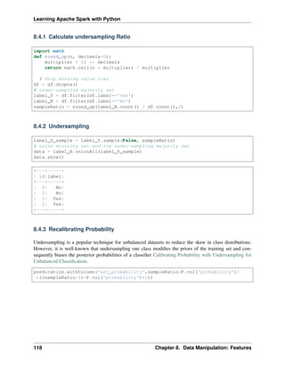
![CHAPTER
NINE
REGRESSION
Chinese proverb
A journey of a thousand miles begins with a single step. – old Chinese proverb
In statistical modeling, regression analysis focuses on investigating the relationship between a dependent
variable and one or more independent variables. Wikipedia Regression analysis
In data mining, Regression is a model to represent the relationship between the value of lable ( or target,
it is numerical variable) and on one or more features (or predictors they can be numerical and categorical
variables).
9.1 Linear Regression
9.1.1 Introduction
Given that a data set { 𝑥𝑖1, . . . , 𝑥𝑖𝑛, 𝑦𝑖}𝑚
𝑖=1 which contains n features (variables) and m samples (data points),
in simple linear regression model for modeling 𝑚 data points with 𝑗 independent variables: 𝑥𝑖𝑗, the formula
is given by:
𝑦𝑖 = 𝛽0 + 𝛽𝑗𝑥𝑖𝑗, where, 𝑖 = 1, · · · 𝑚, 𝑗 = 1, · · · 𝑛.
In matrix notation, the data set is written as X = [𝑥1, · · · , 𝑥𝑛] with 𝑥𝑗 = {𝑥𝑖𝑗}𝑚
𝑖=1, 𝑦 = {𝑦𝑖}𝑚
𝑖=1 (see Fig.
Feature matrix and label) and 𝛽⊤
= {𝛽𝑗}𝑛
𝑗=1. Then the matrix format equation is written as
𝑦 = X𝛽. (9.1)
119](https://image.slidesharecdn.com/pyspark-230429134708-b35c8a19/85/pyspark-pdf-125-320.jpg)
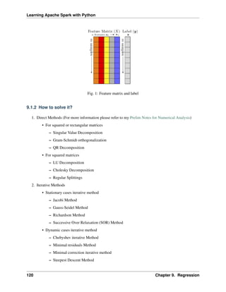
![Learning Apache Spark with Python
– Conjugate Gradients Method
9.1.3 Ordinary Least Squares
In mathematics, (9.1) is a overdetermined system. The method of ordinary least squares can be used to find
an approximate solution to overdetermined systems. For the system overdetermined system (9.1), the least
squares formula is obtained from the problem
min
𝛽
||X𝛽 − 𝑦||, (9.2)
the solution of which can be written with the normal equations:
𝛽 = (X𝑇
X)−1
X𝑇
𝑦 (9.3)
where T indicates a matrix transpose, provided (XT
X)−1
exists (that is, provided X has full column rank).
Note: Actually, (9.3) can be derivated by the following way: multiply X𝑇 on side of (9.1) and then multiply
(X𝑇 X)−1 on both side of the former result. You may also apply the Extreme Value Theorem to (9.2)
and find the solution (9.3).
9.1.4 Gradient Descent
Let’s use the following hypothesis:
ℎ𝛽 = 𝛽0 + 𝛽𝑗𝑥𝑗, where, 𝑗 = 1, · · · 𝑛.
Then, solving (9.2) is equivalent to minimize the following cost fucntion :
9.1.5 Cost Function
𝐽(𝛽) =
1
2𝑚
𝑚
∑︁
𝑖=1
(︁
ℎ𝛽(𝑥(𝑖)
) − 𝑦(𝑖)
)
)︁2
(9.4)
Note: The reason why we prefer to solve (9.4) rather than (9.2) is because (9.4) is convex and it has some
nice properties, such as it’s uniquely solvable and energy stable for small enough learning rate. the interested
reader who has great interest in non-convex cost function (energy) case. is referred to [Feng2016PSD] for
more details.
9.1. Linear Regression 121](https://image.slidesharecdn.com/pyspark-230429134708-b35c8a19/85/pyspark-pdf-127-320.jpg)
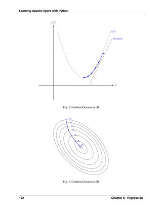
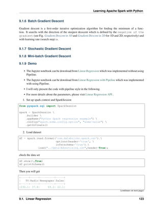
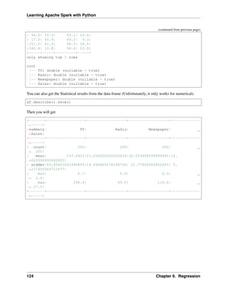
![Learning Apache Spark with Python
Fig. 4: Sales distribution
3. Convert the data to dense vector (features and label)
from pyspark.sql import Row
from pyspark.ml.linalg import Vectors
# I provide two ways to build the features and labels
# method 1 (good for small feature):
#def transData(row):
# return Row(label=row["Sales"],
# features=Vectors.dense([row["TV"],
# row["Radio"],
# row["Newspaper"]]))
# Method 2 (good for large features):
def transData(data):
return data.rdd.map(lambda r: [Vectors.dense(r[:-1]),r[-1]]).toDF(['features',
˓
→'label'])
Note:
You are strongly encouraged to try my get_dummy function for dealing with the categorical
data in comple dataset.
Supervised learning version:
def get_dummy(df,indexCol,categoricalCols,continuousCols,
˓
→labelCol):
(continues on next page)
9.1. Linear Regression 125](https://image.slidesharecdn.com/pyspark-230429134708-b35c8a19/85/pyspark-pdf-131-320.jpg)
![Learning Apache Spark with Python
(continued from previous page)
from pyspark.ml import Pipeline
from pyspark.ml.feature import StringIndexer,
˓
→OneHotEncoder, VectorAssembler
from pyspark.sql.functions import col
indexers = [ StringIndexer(inputCol=c, outputCol="{0}_
˓
→indexed".format(c))
for c in categoricalCols ]
# default setting: dropLast=True
encoders = [ OneHotEncoder(inputCol=indexer.
˓
→getOutputCol(),
outputCol="{0}_encoded".format(indexer.
˓
→getOutputCol()))
for indexer in indexers ]
assembler = VectorAssembler(inputCols=[encoder.
˓
→getOutputCol() for encoder in encoders]
+ continuousCols, outputCol=
˓
→"features")
pipeline = Pipeline(stages=indexers + encoders +
˓
→[assembler])
model=pipeline.fit(df)
data = model.transform(df)
data = data.withColumn('label',col(labelCol))
if indexCol:
return data.select(indexCol,'features','label')
else:
return data.select('features','label')
Unsupervised learning version:
def get_dummy(df,indexCol,categoricalCols,continuousCols):
'''
Get dummy variables and concat with continuous variables
˓
→for unsupervised learning.
:param df: the dataframe
:param categoricalCols: the name list of the categorical
˓
→data
:param continuousCols: the name list of the numerical
˓
→data
:return k: feature matrix
:author: Wenqiang Feng
:email: von198@gmail.com
'''
(continues on next page)
126 Chapter 9. Regression](https://image.slidesharecdn.com/pyspark-230429134708-b35c8a19/85/pyspark-pdf-132-320.jpg)
![Learning Apache Spark with Python
(continued from previous page)
indexers = [ StringIndexer(inputCol=c, outputCol="{0}_
˓
→indexed".format(c))
for c in categoricalCols ]
# default setting: dropLast=True
encoders = [ OneHotEncoder(inputCol=indexer.
˓
→getOutputCol(),
outputCol="{0}_encoded".format(indexer.
˓
→getOutputCol()))
for indexer in indexers ]
assembler = VectorAssembler(inputCols=[encoder.
˓
→getOutputCol() for encoder in encoders]
+ continuousCols, outputCol=
˓
→"features")
pipeline = Pipeline(stages=indexers + encoders +
˓
→[assembler])
model=pipeline.fit(df)
data = model.transform(df)
if indexCol:
return data.select(indexCol,'features')
else:
return data.select('features')
Two in one:
def get_dummy(df,indexCol,categoricalCols,continuousCols,labelCol,
˓
→dropLast=False):
'''
Get dummy variables and concat with continuous variables for ml
˓
→modeling.
:param df: the dataframe
:param categoricalCols: the name list of the categorical data
:param continuousCols: the name list of the numerical data
:param labelCol: the name of label column
:param dropLast: the flag of drop last column
:return: feature matrix
:author: Wenqiang Feng
:email: von198@gmail.com
>>> df = spark.createDataFrame([
(0, "a"),
(1, "b"),
(2, "c"),
(3, "a"),
(4, "a"),
(5, "c")
(continues on next page)
9.1. Linear Regression 127](https://image.slidesharecdn.com/pyspark-230429134708-b35c8a19/85/pyspark-pdf-133-320.jpg)
![Learning Apache Spark with Python
(continued from previous page)
], ["id", "category"])
>>> indexCol = 'id'
>>> categoricalCols = ['category']
>>> continuousCols = []
>>> labelCol = []
>>> mat = get_dummy(df,indexCol,categoricalCols,continuousCols,
˓
→labelCol)
>>> mat.show()
>>>
+---+-------------+
| id| features|
+---+-------------+
| 0|[1.0,0.0,0.0]|
| 1|[0.0,0.0,1.0]|
| 2|[0.0,1.0,0.0]|
| 3|[1.0,0.0,0.0]|
| 4|[1.0,0.0,0.0]|
| 5|[0.0,1.0,0.0]|
+---+-------------+
'''
from pyspark.ml import Pipeline
from pyspark.ml.feature import StringIndexer, OneHotEncoder,
˓
→VectorAssembler
from pyspark.sql.functions import col
indexers = [ StringIndexer(inputCol=c, outputCol="{0}_indexed".
˓
→format(c))
for c in categoricalCols ]
# default setting: dropLast=True
encoders = [ OneHotEncoder(inputCol=indexer.getOutputCol(),
outputCol="{0}_encoded".format(indexer.
˓
→getOutputCol()),dropLast=dropLast)
for indexer in indexers ]
assembler = VectorAssembler(inputCols=[encoder.getOutputCol()
˓
→for encoder in encoders]
+ continuousCols, outputCol="features
˓
→")
pipeline = Pipeline(stages=indexers + encoders + [assembler])
model=pipeline.fit(df)
data = model.transform(df)
if indexCol and labelCol:
# for supervised learning
data = data.withColumn('label',col(labelCol))
(continues on next page)
128 Chapter 9. Regression](https://image.slidesharecdn.com/pyspark-230429134708-b35c8a19/85/pyspark-pdf-134-320.jpg)
![Learning Apache Spark with Python
(continued from previous page)
return data.select(indexCol,'features','label')
elif not indexCol and labelCol:
# for supervised learning
data = data.withColumn('label',col(labelCol))
return data.select('features','label')
elif indexCol and not labelCol:
# for unsupervised learning
return data.select(indexCol,'features')
elif not indexCol and not labelCol:
# for unsupervised learning
return data.select('features')
4. Transform the dataset to DataFrame
transformed= transData(df)
transformed.show(5)
+-----------------+-----+
| features|label|
+-----------------+-----+
|[230.1,37.8,69.2]| 22.1|
| [44.5,39.3,45.1]| 10.4|
| [17.2,45.9,69.3]| 9.3|
|[151.5,41.3,58.5]| 18.5|
|[180.8,10.8,58.4]| 12.9|
+-----------------+-----+
only showing top 5 rows
Note: You will find out that all of the supervised machine learning algorithms in Spark are based on the
features and label (unsupervised machine learning algorithms in Spark are based on the features). That is
to say, you can play with all of the machine learning algorithms in Spark when you get ready the features
and label in pipeline architecture.
5. Deal With Categorical Variables
from pyspark.ml import Pipeline
from pyspark.ml.regression import LinearRegression
from pyspark.ml.feature import VectorIndexer
from pyspark.ml.evaluation import RegressionEvaluator
# Automatically identify categorical features, and index them.
# We specify maxCategories so features with > 4 distinct values are treated
˓
→as continuous.
featureIndexer = VectorIndexer(inputCol="features",
outputCol="indexedFeatures",
maxCategories=4).fit(transformed)
(continues on next page)
9.1. Linear Regression 129](https://image.slidesharecdn.com/pyspark-230429134708-b35c8a19/85/pyspark-pdf-135-320.jpg)
![Learning Apache Spark with Python
(continued from previous page)
data = featureIndexer.transform(transformed)
Now you check your dataset with
data.show(5,True)
you will get
+-----------------+-----+-----------------+
| features|label| indexedFeatures|
+-----------------+-----+-----------------+
|[230.1,37.8,69.2]| 22.1|[230.1,37.8,69.2]|
| [44.5,39.3,45.1]| 10.4| [44.5,39.3,45.1]|
| [17.2,45.9,69.3]| 9.3| [17.2,45.9,69.3]|
|[151.5,41.3,58.5]| 18.5|[151.5,41.3,58.5]|
|[180.8,10.8,58.4]| 12.9|[180.8,10.8,58.4]|
+-----------------+-----+-----------------+
only showing top 5 rows
6. Split the data into training and test sets (40% held out for testing)
# Split the data into training and test sets (40% held out for testing)
(trainingData, testData) = transformed.randomSplit([0.6, 0.4])
You can check your train and test data as follows (In my opinion, it is always to good to keep tracking your
data during prototype pahse):
trainingData.show(5)
testData.show(5)
Then you will get
+---------------+-----+---------------+
| features|label|indexedFeatures|
+---------------+-----+---------------+
| [4.1,11.6,5.7]| 3.2| [4.1,11.6,5.7]|
| [5.4,29.9,9.4]| 5.3| [5.4,29.9,9.4]|
|[7.3,28.1,41.4]| 5.5|[7.3,28.1,41.4]|
|[7.8,38.9,50.6]| 6.6|[7.8,38.9,50.6]|
| [8.6,2.1,1.0]| 4.8| [8.6,2.1,1.0]|
+---------------+-----+---------------+
only showing top 5 rows
+----------------+-----+----------------+
| features|label| indexedFeatures|
+----------------+-----+----------------+
| [0.7,39.6,8.7]| 1.6| [0.7,39.6,8.7]|
| [8.4,27.2,2.1]| 5.7| [8.4,27.2,2.1]|
|[11.7,36.9,45.2]| 7.3|[11.7,36.9,45.2]|
|[13.2,15.9,49.6]| 5.6|[13.2,15.9,49.6]|
(continues on next page)
130 Chapter 9. Regression](https://image.slidesharecdn.com/pyspark-230429134708-b35c8a19/85/pyspark-pdf-136-320.jpg)
![Learning Apache Spark with Python
(continued from previous page)
|[16.9,43.7,89.4]| 8.7|[16.9,43.7,89.4]|
+----------------+-----+----------------+
only showing top 5 rows
7. Fit Ordinary Least Square Regression Model
For more details about the parameters, please visit Linear Regression API .
# Import LinearRegression class
from pyspark.ml.regression import LinearRegression
# Define LinearRegression algorithm
lr = LinearRegression()
8. Pipeline Architecture
# Chain indexer and tree in a Pipeline
pipeline = Pipeline(stages=[featureIndexer, lr])
model = pipeline.fit(trainingData)
9. Summary of the Model
Spark has a poor summary function for data and model. I wrote a summary function which has similar
format as R output for the linear regression in PySpark.
def modelsummary(model):
import numpy as np
print ("Note: the last rows are the information for Intercept")
print ("##","-------------------------------------------------")
print ("##"," Estimate | Std.Error | t Values | P-value")
coef = np.append(list(model.coefficients),model.intercept)
Summary=model.summary
for i in range(len(Summary.pValues)):
print ("##",'{:10.6f}'.format(coef[i]),
'{:10.6f}'.format(Summary.coefficientStandardErrors[i]),
'{:8.3f}'.format(Summary.tValues[i]),
'{:10.6f}'.format(Summary.pValues[i]))
print ("##",'---')
print ("##","Mean squared error: % .6f"
% Summary.meanSquaredError, ", RMSE: % .6f"
% Summary.rootMeanSquaredError )
print ("##","Multiple R-squared: %f" % Summary.r2, ",
Total iterations: %i"% Summary.totalIterations)
modelsummary(model.stages[-1])
You will get the following summary results:
9.1. Linear Regression 131](https://image.slidesharecdn.com/pyspark-230429134708-b35c8a19/85/pyspark-pdf-137-320.jpg)
![Learning Apache Spark with Python
Note: the last rows are the information for Intercept
('##', '-------------------------------------------------')
('##', ' Estimate | Std.Error | t Values | P-value')
('##', ' 0.044186', ' 0.001663', ' 26.573', ' 0.000000')
('##', ' 0.206311', ' 0.010846', ' 19.022', ' 0.000000')
('##', ' 0.001963', ' 0.007467', ' 0.263', ' 0.793113')
('##', ' 2.596154', ' 0.379550', ' 6.840', ' 0.000000')
('##', '---')
('##', 'Mean squared error: 2.588230', ', RMSE: 1.608798')
('##', 'Multiple R-squared: 0.911869', ', Total iterations: 1')
10. Make predictions
# Make predictions.
predictions = model.transform(testData)
# Select example rows to display.
predictions.select("features","label","prediction").show(5)
+----------------+-----+------------------+
| features|label| prediction|
+----------------+-----+------------------+
| [0.7,39.6,8.7]| 1.6| 10.81405928637388|
| [8.4,27.2,2.1]| 5.7| 8.583086404079918|
|[11.7,36.9,45.2]| 7.3|10.814712818232422|
|[13.2,15.9,49.6]| 5.6| 6.557106943899219|
|[16.9,43.7,89.4]| 8.7|12.534151375058645|
+----------------+-----+------------------+
only showing top 5 rows
9. Evaluation
from pyspark.ml.evaluation import RegressionEvaluator
# Select (prediction, true label) and compute test error
evaluator = RegressionEvaluator(labelCol="label",
predictionCol="prediction",
metricName="rmse")
rmse = evaluator.evaluate(predictions)
print("Root Mean Squared Error (RMSE) on test data = %g" % rmse)
The final Root Mean Squared Error (RMSE) is as follows:
Root Mean Squared Error (RMSE) on test data = 1.63114
You can also check the 𝑅2 value for the test data:
y_true = predictions.select("label").toPandas()
y_pred = predictions.select("prediction").toPandas()
import sklearn.metrics
(continues on next page)
132 Chapter 9. Regression](https://image.slidesharecdn.com/pyspark-230429134708-b35c8a19/85/pyspark-pdf-138-320.jpg)
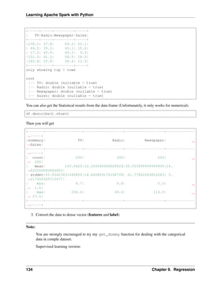
![Learning Apache Spark with Python
def get_dummy(df,indexCol,categoricalCols,continuousCols,
˓
→labelCol):
from pyspark.ml import Pipeline
from pyspark.ml.feature import StringIndexer,
˓
→OneHotEncoder, VectorAssembler
from pyspark.sql.functions import col
indexers = [ StringIndexer(inputCol=c, outputCol="{0}_
˓
→indexed".format(c))
for c in categoricalCols ]
# default setting: dropLast=True
encoders = [ OneHotEncoder(inputCol=indexer.
˓
→getOutputCol(),
outputCol="{0}_encoded".format(indexer.
˓
→getOutputCol()))
for indexer in indexers ]
assembler = VectorAssembler(inputCols=[encoder.
˓
→getOutputCol() for encoder in encoders]
+ continuousCols, outputCol=
˓
→"features")
pipeline = Pipeline(stages=indexers + encoders +
˓
→[assembler])
model=pipeline.fit(df)
data = model.transform(df)
data = data.withColumn('label',col(labelCol))
if indexCol:
return data.select(indexCol,'features','label')
else:
return data.select('features','label')
Unsupervised learning version:
def get_dummy(df,indexCol,categoricalCols,continuousCols):
'''
Get dummy variables and concat with continuous variables
˓
→for unsupervised learning.
:param df: the dataframe
:param categoricalCols: the name list of the categorical
˓
→data
:param continuousCols: the name list of the numerical
˓
→data
:return k: feature matrix
:author: Wenqiang Feng
:email: von198@gmail.com
(continues on next page)
9.2. Generalized linear regression 135](https://image.slidesharecdn.com/pyspark-230429134708-b35c8a19/85/pyspark-pdf-141-320.jpg)
![Learning Apache Spark with Python
(continued from previous page)
'''
indexers = [ StringIndexer(inputCol=c, outputCol="{0}_
˓
→indexed".format(c))
for c in categoricalCols ]
# default setting: dropLast=True
encoders = [ OneHotEncoder(inputCol=indexer.
˓
→getOutputCol(),
outputCol="{0}_encoded".format(indexer.
˓
→getOutputCol()))
for indexer in indexers ]
assembler = VectorAssembler(inputCols=[encoder.
˓
→getOutputCol() for encoder in encoders]
+ continuousCols, outputCol=
˓
→"features")
pipeline = Pipeline(stages=indexers + encoders +
˓
→[assembler])
model=pipeline.fit(df)
data = model.transform(df)
if indexCol:
return data.select(indexCol,'features')
else:
return data.select('features')
Two in one:
def get_dummy(df,indexCol,categoricalCols,continuousCols,labelCol,
˓
→dropLast=False):
'''
Get dummy variables and concat with continuous variables for ml
˓
→modeling.
:param df: the dataframe
:param categoricalCols: the name list of the categorical data
:param continuousCols: the name list of the numerical data
:param labelCol: the name of label column
:param dropLast: the flag of drop last column
:return: feature matrix
:author: Wenqiang Feng
:email: von198@gmail.com
>>> df = spark.createDataFrame([
(0, "a"),
(1, "b"),
(2, "c"),
(3, "a"),
(continues on next page)
136 Chapter 9. Regression](https://image.slidesharecdn.com/pyspark-230429134708-b35c8a19/85/pyspark-pdf-142-320.jpg)
![Learning Apache Spark with Python
(continued from previous page)
(4, "a"),
(5, "c")
], ["id", "category"])
>>> indexCol = 'id'
>>> categoricalCols = ['category']
>>> continuousCols = []
>>> labelCol = []
>>> mat = get_dummy(df,indexCol,categoricalCols,continuousCols,
˓
→labelCol)
>>> mat.show()
>>>
+---+-------------+
| id| features|
+---+-------------+
| 0|[1.0,0.0,0.0]|
| 1|[0.0,0.0,1.0]|
| 2|[0.0,1.0,0.0]|
| 3|[1.0,0.0,0.0]|
| 4|[1.0,0.0,0.0]|
| 5|[0.0,1.0,0.0]|
+---+-------------+
'''
from pyspark.ml import Pipeline
from pyspark.ml.feature import StringIndexer, OneHotEncoder,
˓
→VectorAssembler
from pyspark.sql.functions import col
indexers = [ StringIndexer(inputCol=c, outputCol="{0}_indexed".
˓
→format(c))
for c in categoricalCols ]
# default setting: dropLast=True
encoders = [ OneHotEncoder(inputCol=indexer.getOutputCol(),
outputCol="{0}_encoded".format(indexer.
˓
→getOutputCol()),dropLast=dropLast)
for indexer in indexers ]
assembler = VectorAssembler(inputCols=[encoder.getOutputCol()
˓
→for encoder in encoders]
+ continuousCols, outputCol="features
˓
→")
pipeline = Pipeline(stages=indexers + encoders + [assembler])
model=pipeline.fit(df)
data = model.transform(df)
if indexCol and labelCol:
(continues on next page)
9.2. Generalized linear regression 137](https://image.slidesharecdn.com/pyspark-230429134708-b35c8a19/85/pyspark-pdf-143-320.jpg)
![Learning Apache Spark with Python
(continued from previous page)
# for supervised learning
data = data.withColumn('label',col(labelCol))
return data.select(indexCol,'features','label')
elif not indexCol and labelCol:
# for supervised learning
data = data.withColumn('label',col(labelCol))
return data.select('features','label')
elif indexCol and not labelCol:
# for unsupervised learning
return data.select(indexCol,'features')
elif not indexCol and not labelCol:
# for unsupervised learning
return data.select('features')
from pyspark.sql import Row
from pyspark.ml.linalg import Vectors
# I provide two ways to build the features and labels
# method 1 (good for small feature):
#def transData(row):
# return Row(label=row["Sales"],
# features=Vectors.dense([row["TV"],
# row["Radio"],
# row["Newspaper"]]))
# Method 2 (good for large features):
def transData(data):
return data.rdd.map(lambda r: [Vectors.dense(r[:-1]),r[-1]]).toDF(['features',
˓
→'label'])
transformed= transData(df)
transformed.show(5)
+-----------------+-----+
| features|label|
+-----------------+-----+
|[230.1,37.8,69.2]| 22.1|
| [44.5,39.3,45.1]| 10.4|
| [17.2,45.9,69.3]| 9.3|
|[151.5,41.3,58.5]| 18.5|
|[180.8,10.8,58.4]| 12.9|
+-----------------+-----+
only showing top 5 rows
Note: You will find out that all of the machine learning algorithms in Spark are based on the features and
label. That is to say, you can play with all of the machine learning algorithms in Spark when you get ready
138 Chapter 9. Regression](https://image.slidesharecdn.com/pyspark-230429134708-b35c8a19/85/pyspark-pdf-144-320.jpg)
![Learning Apache Spark with Python
the features and label.
4. Convert the data to dense vector
# convert the data to dense vector
def transData(data):
return data.rdd.map(lambda r: [r[-1], Vectors.dense(r[:-1])]).
toDF(['label','features'])
from pyspark.sql import Row
from pyspark.ml.linalg import Vectors
data= transData(df)
data.show()
5. Deal with the Categorical variables
from pyspark.ml import Pipeline
from pyspark.ml.regression import LinearRegression
from pyspark.ml.feature import VectorIndexer
from pyspark.ml.evaluation import RegressionEvaluator
# Automatically identify categorical features, and index them.
# We specify maxCategories so features with > 4
# distinct values are treated as continuous.
featureIndexer = VectorIndexer(inputCol="features",
outputCol="indexedFeatures",
maxCategories=4).fit(transformed)
data = featureIndexer.transform(transformed)
When you check you data at this point, you will get
+-----------------+-----+-----------------+
| features|label| indexedFeatures|
+-----------------+-----+-----------------+
|[230.1,37.8,69.2]| 22.1|[230.1,37.8,69.2]|
| [44.5,39.3,45.1]| 10.4| [44.5,39.3,45.1]|
| [17.2,45.9,69.3]| 9.3| [17.2,45.9,69.3]|
|[151.5,41.3,58.5]| 18.5|[151.5,41.3,58.5]|
|[180.8,10.8,58.4]| 12.9|[180.8,10.8,58.4]|
+-----------------+-----+-----------------+
only showing top 5 rows
6. Split the data into training and test sets (40% held out for testing)
# Split the data into training and test sets (40% held out for testing)
(trainingData, testData) = transformed.randomSplit([0.6, 0.4])
You can check your train and test data as follows (In my opinion, it is always to good to keep tracking your
data during prototype phase):
9.2. Generalized linear regression 139](https://image.slidesharecdn.com/pyspark-230429134708-b35c8a19/85/pyspark-pdf-145-320.jpg)
![Learning Apache Spark with Python
trainingData.show(5)
testData.show(5)
Then you will get
+----------------+-----+----------------+
| features|label| indexedFeatures|
+----------------+-----+----------------+
| [5.4,29.9,9.4]| 5.3| [5.4,29.9,9.4]|
| [7.8,38.9,50.6]| 6.6| [7.8,38.9,50.6]|
| [8.4,27.2,2.1]| 5.7| [8.4,27.2,2.1]|
| [8.7,48.9,75.0]| 7.2| [8.7,48.9,75.0]|
|[11.7,36.9,45.2]| 7.3|[11.7,36.9,45.2]|
+----------------+-----+----------------+
only showing top 5 rows
+---------------+-----+---------------+
| features|label|indexedFeatures|
+---------------+-----+---------------+
| [0.7,39.6,8.7]| 1.6| [0.7,39.6,8.7]|
| [4.1,11.6,5.7]| 3.2| [4.1,11.6,5.7]|
|[7.3,28.1,41.4]| 5.5|[7.3,28.1,41.4]|
| [8.6,2.1,1.0]| 4.8| [8.6,2.1,1.0]|
|[17.2,4.1,31.6]| 5.9|[17.2,4.1,31.6]|
+---------------+-----+---------------+
only showing top 5 rows
7. Fit Generalized Linear Regression Model
# Import LinearRegression class
from pyspark.ml.regression import GeneralizedLinearRegression
# Define LinearRegression algorithm
glr = GeneralizedLinearRegression(family="gaussian", link="identity",
maxIter=10, regParam=0.3)
8. Pipeline Architecture
# Chain indexer and tree in a Pipeline
pipeline = Pipeline(stages=[featureIndexer, glr])
model = pipeline.fit(trainingData)
9. Summary of the Model
Spark has a poor summary function for data and model. I wrote a summary function which has similar
format as R output for the linear regression in PySpark.
def modelsummary(model):
import numpy as np
print ("Note: the last rows are the information for Intercept")
print ("##","-------------------------------------------------")
(continues on next page)
140 Chapter 9. Regression](https://image.slidesharecdn.com/pyspark-230429134708-b35c8a19/85/pyspark-pdf-146-320.jpg)
![Learning Apache Spark with Python
(continued from previous page)
print ("##"," Estimate | Std.Error | t Values | P-value")
coef = np.append(list(model.coefficients),model.intercept)
Summary=model.summary
for i in range(len(Summary.pValues)):
print ("##",'{:10.6f}'.format(coef[i]),
'{:10.6f}'.format(Summary.coefficientStandardErrors[i]),
'{:8.3f}'.format(Summary.tValues[i]),
'{:10.6f}'.format(Summary.pValues[i]))
print ("##",'---')
# print ("##","Mean squared error: % .6f"
# % Summary.meanSquaredError, ", RMSE: % .6f"
# % Summary.rootMeanSquaredError )
# print ("##","Multiple R-squared: %f" % Summary.r2, ",
# Total iterations: %i"% Summary.totalIterations)
modelsummary(model.stages[-1])
You will get the following summary results:
Note: the last rows are the information for Intercept
('##', '-------------------------------------------------')
('##', ' Estimate | Std.Error | t Values | P-value')
('##', ' 0.042857', ' 0.001668', ' 25.692', ' 0.000000')
('##', ' 0.199922', ' 0.009881', ' 20.232', ' 0.000000')
('##', ' -0.001957', ' 0.006917', ' -0.283', ' 0.777757')
('##', ' 3.007515', ' 0.406389', ' 7.401', ' 0.000000')
('##', '---')
10. Make predictions
# Make predictions.
predictions = model.transform(testData)
# Select example rows to display.
predictions.select("features","label","predictedLabel").show(5)
+---------------+-----+------------------+
| features|label| prediction|
+---------------+-----+------------------+
| [0.7,39.6,8.7]| 1.6|10.937383732327625|
| [4.1,11.6,5.7]| 3.2| 5.491166258750164|
|[7.3,28.1,41.4]| 5.5| 8.8571603947873|
| [8.6,2.1,1.0]| 4.8| 3.793966281660073|
|[17.2,4.1,31.6]| 5.9| 4.502507124763654|
+---------------+-----+------------------+
only showing top 5 rows
11. Evaluation
9.2. Generalized linear regression 141](https://image.slidesharecdn.com/pyspark-230429134708-b35c8a19/85/pyspark-pdf-147-320.jpg)
![Learning Apache Spark with Python
(continued from previous page)
3. Convert the data to dense vector (features and label)
Note:
You are strongly encouraged to try my get_dummy function for dealing with the categorical
data in comple dataset.
Supervised learning version:
def get_dummy(df,indexCol,categoricalCols,continuousCols,
˓
→labelCol):
from pyspark.ml import Pipeline
from pyspark.ml.feature import StringIndexer,
˓
→OneHotEncoder, VectorAssembler
from pyspark.sql.functions import col
indexers = [ StringIndexer(inputCol=c, outputCol="{0}_
˓
→indexed".format(c))
for c in categoricalCols ]
# default setting: dropLast=True
encoders = [ OneHotEncoder(inputCol=indexer.
˓
→getOutputCol(),
outputCol="{0}_encoded".format(indexer.
˓
→getOutputCol()))
for indexer in indexers ]
assembler = VectorAssembler(inputCols=[encoder.
˓
→getOutputCol() for encoder in encoders]
+ continuousCols, outputCol=
˓
→"features")
pipeline = Pipeline(stages=indexers + encoders +
˓
→[assembler])
model=pipeline.fit(df)
data = model.transform(df)
data = data.withColumn('label',col(labelCol))
return data.select(indexCol,'features','label')
Unsupervised learning version:
def get_dummy(df,indexCol,categoricalCols,continuousCols):
'''
Get dummy variables and concat with continuous variables
˓
→for unsupervised learning.
(continues on next page)
144 Chapter 9. Regression](https://image.slidesharecdn.com/pyspark-230429134708-b35c8a19/85/pyspark-pdf-150-320.jpg)
![Learning Apache Spark with Python
(continued from previous page)
:param df: the dataframe
:param categoricalCols: the name list of the categorical
˓
→data
:param continuousCols: the name list of the numerical
˓
→data
:return k: feature matrix
:author: Wenqiang Feng
:email: von198@gmail.com
'''
indexers = [ StringIndexer(inputCol=c, outputCol="{0}_
˓
→indexed".format(c))
for c in categoricalCols ]
# default setting: dropLast=True
encoders = [ OneHotEncoder(inputCol=indexer.
˓
→getOutputCol(),
outputCol="{0}_encoded".format(indexer.
˓
→getOutputCol()))
for indexer in indexers ]
assembler = VectorAssembler(inputCols=[encoder.
˓
→getOutputCol() for encoder in encoders]
+ continuousCols, outputCol=
˓
→"features")
pipeline = Pipeline(stages=indexers + encoders +
˓
→[assembler])
model=pipeline.fit(df)
data = model.transform(df)
return data.select(indexCol,'features')
Two in one:
def get_dummy(df,indexCol,categoricalCols,continuousCols,labelCol,
˓
→dropLast=False):
'''
Get dummy variables and concat with continuous variables for ml
˓
→modeling.
:param df: the dataframe
:param categoricalCols: the name list of the categorical data
:param continuousCols: the name list of the numerical data
:param labelCol: the name of label column
:param dropLast: the flag of drop last column
:return: feature matrix
:author: Wenqiang Feng
:email: von198@gmail.com
(continues on next page)
9.3. Decision tree Regression 145](https://image.slidesharecdn.com/pyspark-230429134708-b35c8a19/85/pyspark-pdf-151-320.jpg)
![Learning Apache Spark with Python
(continued from previous page)
>>> df = spark.createDataFrame([
(0, "a"),
(1, "b"),
(2, "c"),
(3, "a"),
(4, "a"),
(5, "c")
], ["id", "category"])
>>> indexCol = 'id'
>>> categoricalCols = ['category']
>>> continuousCols = []
>>> labelCol = []
>>> mat = get_dummy(df,indexCol,categoricalCols,continuousCols,
˓
→labelCol)
>>> mat.show()
>>>
+---+-------------+
| id| features|
+---+-------------+
| 0|[1.0,0.0,0.0]|
| 1|[0.0,0.0,1.0]|
| 2|[0.0,1.0,0.0]|
| 3|[1.0,0.0,0.0]|
| 4|[1.0,0.0,0.0]|
| 5|[0.0,1.0,0.0]|
+---+-------------+
'''
from pyspark.ml import Pipeline
from pyspark.ml.feature import StringIndexer, OneHotEncoder,
˓
→VectorAssembler
from pyspark.sql.functions import col
indexers = [ StringIndexer(inputCol=c, outputCol="{0}_indexed".
˓
→format(c))
for c in categoricalCols ]
# default setting: dropLast=True
encoders = [ OneHotEncoder(inputCol=indexer.getOutputCol(),
outputCol="{0}_encoded".format(indexer.
˓
→getOutputCol()),dropLast=dropLast)
for indexer in indexers ]
assembler = VectorAssembler(inputCols=[encoder.getOutputCol()
˓
→for encoder in encoders]
+ continuousCols, outputCol="features
˓
→")
(continues on next page)
146 Chapter 9. Regression](https://image.slidesharecdn.com/pyspark-230429134708-b35c8a19/85/pyspark-pdf-152-320.jpg)
![Learning Apache Spark with Python
(continued from previous page)
pipeline = Pipeline(stages=indexers + encoders + [assembler])
model=pipeline.fit(df)
data = model.transform(df)
if indexCol and labelCol:
# for supervised learning
data = data.withColumn('label',col(labelCol))
return data.select(indexCol,'features','label')
elif not indexCol and labelCol:
# for supervised learning
data = data.withColumn('label',col(labelCol))
return data.select('features','label')
elif indexCol and not labelCol:
# for unsupervised learning
return data.select(indexCol,'features')
elif not indexCol and not labelCol:
# for unsupervised learning
return data.select('features')
from pyspark.sql import Row
from pyspark.ml.linalg import Vectors
# I provide two ways to build the features and labels
# method 1 (good for small feature):
#def transData(row):
# return Row(label=row["Sales"],
# features=Vectors.dense([row["TV"],
# row["Radio"],
# row["Newspaper"]]))
# Method 2 (good for large features):
def transData(data):
return data.rdd.map(lambda r: [Vectors.dense(r[:-1]),r[-1]]).toDF(['features',
˓
→'label'])
transformed= transData(df)
transformed.show(5)
+-----------------+-----+
| features|label|
+-----------------+-----+
|[230.1,37.8,69.2]| 22.1|
| [44.5,39.3,45.1]| 10.4|
| [17.2,45.9,69.3]| 9.3|
|[151.5,41.3,58.5]| 18.5|
|[180.8,10.8,58.4]| 12.9|
+-----------------+-----+
only showing top 5 rows
9.3. Decision tree Regression 147](https://image.slidesharecdn.com/pyspark-230429134708-b35c8a19/85/pyspark-pdf-153-320.jpg)
![Learning Apache Spark with Python
Note: You will find out that all of the machine learning algorithms in Spark are based on the features and
label. That is to say, you can play with all of the machine learning algorithms in Spark when you get ready
the features and label.
4. Convert the data to dense vector
# convert the data to dense vector
def transData(data):
return data.rdd.map(lambda r: [r[-1], Vectors.dense(r[:-1])]).
toDF(['label','features'])
transformed = transData(df)
transformed.show(5)
5. Deal with the Categorical variables
from pyspark.ml import Pipeline
from pyspark.ml.regression import LinearRegression
from pyspark.ml.feature import VectorIndexer
from pyspark.ml.evaluation import RegressionEvaluator
# Automatically identify categorical features, and index them.
# We specify maxCategories so features with > 4
# distinct values are treated as continuous.
featureIndexer = VectorIndexer(inputCol="features",
outputCol="indexedFeatures",
maxCategories=4).fit(transformed)
data = featureIndexer.transform(transformed)
When you check you data at this point, you will get
+-----------------+-----+-----------------+
| features|label| indexedFeatures|
+-----------------+-----+-----------------+
|[230.1,37.8,69.2]| 22.1|[230.1,37.8,69.2]|
| [44.5,39.3,45.1]| 10.4| [44.5,39.3,45.1]|
| [17.2,45.9,69.3]| 9.3| [17.2,45.9,69.3]|
|[151.5,41.3,58.5]| 18.5|[151.5,41.3,58.5]|
|[180.8,10.8,58.4]| 12.9|[180.8,10.8,58.4]|
+-----------------+-----+-----------------+
only showing top 5 rows
6. Split the data into training and test sets (40% held out for testing)
# Split the data into training and test sets (40% held out for testing)
(trainingData, testData) = transformed.randomSplit([0.6, 0.4])
You can check your train and test data as follows (In my opinion, it is always to good to keep tracking your
data during prototype pahse):
148 Chapter 9. Regression](https://image.slidesharecdn.com/pyspark-230429134708-b35c8a19/85/pyspark-pdf-154-320.jpg)
![Learning Apache Spark with Python
trainingData.show(5)
testData.show(5)
Then you will get
+---------------+-----+---------------+
| features|label|indexedFeatures|
+---------------+-----+---------------+
| [4.1,11.6,5.7]| 3.2| [4.1,11.6,5.7]|
|[7.3,28.1,41.4]| 5.5|[7.3,28.1,41.4]|
| [8.4,27.2,2.1]| 5.7| [8.4,27.2,2.1]|
| [8.6,2.1,1.0]| 4.8| [8.6,2.1,1.0]|
|[8.7,48.9,75.0]| 7.2|[8.7,48.9,75.0]|
+---------------+-----+---------------+
only showing top 5 rows
+----------------+-----+----------------+
| features|label| indexedFeatures|
+----------------+-----+----------------+
| [0.7,39.6,8.7]| 1.6| [0.7,39.6,8.7]|
| [5.4,29.9,9.4]| 5.3| [5.4,29.9,9.4]|
| [7.8,38.9,50.6]| 6.6| [7.8,38.9,50.6]|
|[17.2,45.9,69.3]| 9.3|[17.2,45.9,69.3]|
|[18.7,12.1,23.4]| 6.7|[18.7,12.1,23.4]|
+----------------+-----+----------------+
only showing top 5 rows
7. Fit Decision Tree Regression Model
from pyspark.ml.regression import DecisionTreeRegressor
# Train a DecisionTree model.
dt = DecisionTreeRegressor(featuresCol="indexedFeatures")
8. Pipeline Architecture
# Chain indexer and tree in a Pipeline
pipeline = Pipeline(stages=[featureIndexer, dt])
model = pipeline.fit(trainingData)
9. Make predictions
# Make predictions.
predictions = model.transform(testData)
# Select example rows to display.
predictions.select("features","label","predictedLabel").show(5)
+----------+-----+----------------+
|prediction|label| features|
(continues on next page)
9.3. Decision tree Regression 149](https://image.slidesharecdn.com/pyspark-230429134708-b35c8a19/85/pyspark-pdf-155-320.jpg)
![Learning Apache Spark with Python
(continued from previous page)
+----------+-----+----------------+
| 7.2| 1.6| [0.7,39.6,8.7]|
| 7.3| 5.3| [5.4,29.9,9.4]|
| 7.2| 6.6| [7.8,38.9,50.6]|
| 8.64| 9.3|[17.2,45.9,69.3]|
| 6.45| 6.7|[18.7,12.1,23.4]|
+----------+-----+----------------+
only showing top 5 rows
10. Evaluation
from pyspark.ml.evaluation import RegressionEvaluator
from pyspark.ml.evaluation import RegressionEvaluator
# Select (prediction, true label) and compute test error
evaluator = RegressionEvaluator(labelCol="label",
predictionCol="prediction",
metricName="rmse")
rmse = evaluator.evaluate(predictions)
print("Root Mean Squared Error (RMSE) on test data = %g" % rmse)
The final Root Mean Squared Error (RMSE) is as follows:
Root Mean Squared Error (RMSE) on test data = 1.50999
y_true = predictions.select("label").toPandas()
y_pred = predictions.select("prediction").toPandas()
import sklearn.metrics
r2_score = sklearn.metrics.r2_score(y_true, y_pred)
print('r2_score: {0}'.format(r2_score))
Then you will get the 𝑅2 value:
r2_score: 0.911024318967
You may also check the importance of the features:
model.stages[1].featureImportances
The you will get the weight for each features
SparseVector(3, {0: 0.6811, 1: 0.3187, 2: 0.0002})
150 Chapter 9. Regression](https://image.slidesharecdn.com/pyspark-230429134708-b35c8a19/85/pyspark-pdf-156-320.jpg)
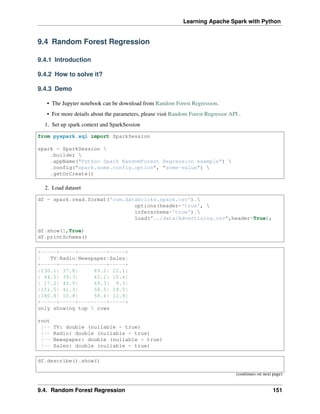
![Learning Apache Spark with Python
(continued from previous page)
+-------+-----------------+------------------+------------------+-------------
˓
→-----+
|summary| TV| Radio| Newspaper|
˓
→Sales|
+-------+-----------------+------------------+------------------+-------------
˓
→-----+
| count| 200| 200| 200|
˓
→ 200|
| mean| 147.0425|23.264000000000024|30.553999999999995|14.
˓
→022500000000003|
| stddev|85.85423631490805|14.846809176168728| 21.77862083852283| 5.
˓
→217456565710477|
| min| 0.7| 0.0| 0.3|
˓
→ 1.6|
| max| 296.4| 49.6| 114.0|
˓
→ 27.0|
+-------+-----------------+------------------+------------------+-------------
˓
→-----+
3. Convert the data to dense vector (features and label)
Note:
You are strongly encouraged to try my get_dummy function for dealing with the categorical
data in comple dataset.
Supervised learning version:
def get_dummy(df,indexCol,categoricalCols,continuousCols,
˓
→labelCol):
from pyspark.ml import Pipeline
from pyspark.ml.feature import StringIndexer,
˓
→OneHotEncoder, VectorAssembler
from pyspark.sql.functions import col
indexers = [ StringIndexer(inputCol=c, outputCol="{0}_
˓
→indexed".format(c))
for c in categoricalCols ]
# default setting: dropLast=True
encoders = [ OneHotEncoder(inputCol=indexer.
˓
→getOutputCol(),
outputCol="{0}_encoded".format(indexer.
˓
→getOutputCol()))
for indexer in indexers ]
assembler = VectorAssembler(inputCols=[encoder.
˓
→getOutputCol() for encoder in encoders]
+ continuousCols, outputCol=
˓
→"features")
(continues on next page)
152 Chapter 9. Regression](https://image.slidesharecdn.com/pyspark-230429134708-b35c8a19/85/pyspark-pdf-158-320.jpg)
![Learning Apache Spark with Python
(continued from previous page)
pipeline = Pipeline(stages=indexers + encoders +
˓
→[assembler])
model=pipeline.fit(df)
data = model.transform(df)
data = data.withColumn('label',col(labelCol))
return data.select(indexCol,'features','label')
Unsupervised learning version:
def get_dummy(df,indexCol,categoricalCols,continuousCols):
'''
Get dummy variables and concat with continuous variables
˓
→for unsupervised learning.
:param df: the dataframe
:param categoricalCols: the name list of the categorical
˓
→data
:param continuousCols: the name list of the numerical
˓
→data
:return k: feature matrix
:author: Wenqiang Feng
:email: von198@gmail.com
'''
indexers = [ StringIndexer(inputCol=c, outputCol="{0}_
˓
→indexed".format(c))
for c in categoricalCols ]
# default setting: dropLast=True
encoders = [ OneHotEncoder(inputCol=indexer.
˓
→getOutputCol(),
outputCol="{0}_encoded".format(indexer.
˓
→getOutputCol()))
for indexer in indexers ]
assembler = VectorAssembler(inputCols=[encoder.
˓
→getOutputCol() for encoder in encoders]
+ continuousCols, outputCol=
˓
→"features")
pipeline = Pipeline(stages=indexers + encoders +
˓
→[assembler])
model=pipeline.fit(df)
data = model.transform(df)
return data.select(indexCol,'features')
9.4. Random Forest Regression 153](https://image.slidesharecdn.com/pyspark-230429134708-b35c8a19/85/pyspark-pdf-159-320.jpg)
![Learning Apache Spark with Python
Two in one:
def get_dummy(df,indexCol,categoricalCols,continuousCols,labelCol,
˓
→dropLast=False):
'''
Get dummy variables and concat with continuous variables for ml
˓
→modeling.
:param df: the dataframe
:param categoricalCols: the name list of the categorical data
:param continuousCols: the name list of the numerical data
:param labelCol: the name of label column
:param dropLast: the flag of drop last column
:return: feature matrix
:author: Wenqiang Feng
:email: von198@gmail.com
>>> df = spark.createDataFrame([
(0, "a"),
(1, "b"),
(2, "c"),
(3, "a"),
(4, "a"),
(5, "c")
], ["id", "category"])
>>> indexCol = 'id'
>>> categoricalCols = ['category']
>>> continuousCols = []
>>> labelCol = []
>>> mat = get_dummy(df,indexCol,categoricalCols,continuousCols,
˓
→labelCol)
>>> mat.show()
>>>
+---+-------------+
| id| features|
+---+-------------+
| 0|[1.0,0.0,0.0]|
| 1|[0.0,0.0,1.0]|
| 2|[0.0,1.0,0.0]|
| 3|[1.0,0.0,0.0]|
| 4|[1.0,0.0,0.0]|
| 5|[0.0,1.0,0.0]|
+---+-------------+
'''
from pyspark.ml import Pipeline
from pyspark.ml.feature import StringIndexer, OneHotEncoder,
˓
→VectorAssembler
from pyspark.sql.functions import col
(continues on next page)
154 Chapter 9. Regression](https://image.slidesharecdn.com/pyspark-230429134708-b35c8a19/85/pyspark-pdf-160-320.jpg)
![Learning Apache Spark with Python
(continued from previous page)
indexers = [ StringIndexer(inputCol=c, outputCol="{0}_indexed".
˓
→format(c))
for c in categoricalCols ]
# default setting: dropLast=True
encoders = [ OneHotEncoder(inputCol=indexer.getOutputCol(),
outputCol="{0}_encoded".format(indexer.
˓
→getOutputCol()),dropLast=dropLast)
for indexer in indexers ]
assembler = VectorAssembler(inputCols=[encoder.getOutputCol()
˓
→for encoder in encoders]
+ continuousCols, outputCol="features
˓
→")
pipeline = Pipeline(stages=indexers + encoders + [assembler])
model=pipeline.fit(df)
data = model.transform(df)
if indexCol and labelCol:
# for supervised learning
data = data.withColumn('label',col(labelCol))
return data.select(indexCol,'features','label')
elif not indexCol and labelCol:
# for supervised learning
data = data.withColumn('label',col(labelCol))
return data.select('features','label')
elif indexCol and not labelCol:
# for unsupervised learning
return data.select(indexCol,'features')
elif not indexCol and not labelCol:
# for unsupervised learning
return data.select('features')
from pyspark.sql import Row
from pyspark.ml.linalg import Vectors
# convert the data to dense vector
#def transData(row):
# return Row(label=row["Sales"],
# features=Vectors.dense([row["TV"],
# row["Radio"],
# row["Newspaper"]]))
def transData(data):
return data.rdd.map(lambda r: [Vectors.dense(r[:-1]),r[-1]]).toDF([
˓
→'features','label'])
4. Convert the data to dense vector
9.4. Random Forest Regression 155](https://image.slidesharecdn.com/pyspark-230429134708-b35c8a19/85/pyspark-pdf-161-320.jpg)
![Learning Apache Spark with Python
transformed= transData(df)
transformed.show(5)
+-----------------+-----+
| features|label|
+-----------------+-----+
|[230.1,37.8,69.2]| 22.1|
| [44.5,39.3,45.1]| 10.4|
| [17.2,45.9,69.3]| 9.3|
|[151.5,41.3,58.5]| 18.5|
|[180.8,10.8,58.4]| 12.9|
+-----------------+-----+
only showing top 5 rows
5. Deal with the Categorical variables
from pyspark.ml import Pipeline
from pyspark.ml.regression import LinearRegression
from pyspark.ml.feature import VectorIndexer
from pyspark.ml.evaluation import RegressionEvaluator
featureIndexer = VectorIndexer(inputCol="features",
outputCol="indexedFeatures",
maxCategories=4).fit(transformed)
data = featureIndexer.transform(transformed)
data.show(5,True)
+-----------------+-----+-----------------+
| features|label| indexedFeatures|
+-----------------+-----+-----------------+
|[230.1,37.8,69.2]| 22.1|[230.1,37.8,69.2]|
| [44.5,39.3,45.1]| 10.4| [44.5,39.3,45.1]|
| [17.2,45.9,69.3]| 9.3| [17.2,45.9,69.3]|
|[151.5,41.3,58.5]| 18.5|[151.5,41.3,58.5]|
|[180.8,10.8,58.4]| 12.9|[180.8,10.8,58.4]|
+-----------------+-----+-----------------+
only showing top 5 rows
6. Split the data into training and test sets (40% held out for testing)
# Split the data into training and test sets (40% held out for testing)
(trainingData, testData) = data.randomSplit([0.6, 0.4])
trainingData.show(5)
testData.show(5)
+----------------+-----+----------------+
| features|label| indexedFeatures|
+----------------+-----+----------------+
| [0.7,39.6,8.7]| 1.6| [0.7,39.6,8.7]|
(continues on next page)
156 Chapter 9. Regression](https://image.slidesharecdn.com/pyspark-230429134708-b35c8a19/85/pyspark-pdf-162-320.jpg)
![Learning Apache Spark with Python
(continued from previous page)
| [8.6,2.1,1.0]| 4.8| [8.6,2.1,1.0]|
| [8.7,48.9,75.0]| 7.2| [8.7,48.9,75.0]|
|[11.7,36.9,45.2]| 7.3|[11.7,36.9,45.2]|
|[13.2,15.9,49.6]| 5.6|[13.2,15.9,49.6]|
+----------------+-----+----------------+
only showing top 5 rows
+---------------+-----+---------------+
| features|label|indexedFeatures|
+---------------+-----+---------------+
| [4.1,11.6,5.7]| 3.2| [4.1,11.6,5.7]|
| [5.4,29.9,9.4]| 5.3| [5.4,29.9,9.4]|
|[7.3,28.1,41.4]| 5.5|[7.3,28.1,41.4]|
|[7.8,38.9,50.6]| 6.6|[7.8,38.9,50.6]|
| [8.4,27.2,2.1]| 5.7| [8.4,27.2,2.1]|
+---------------+-----+---------------+
only showing top 5 rows
7. Fit RandomForest Regression Model
# Import LinearRegression class
from pyspark.ml.regression import RandomForestRegressor
# Define LinearRegression algorithm
rf = RandomForestRegressor() # featuresCol="indexedFeatures",numTrees=2,
˓
→maxDepth=2, seed=42
Note: If you decide to use the indexedFeatures features, you need to add the parameter
featuresCol="indexedFeatures".
8. Pipeline Architecture
# Chain indexer and tree in a Pipeline
pipeline = Pipeline(stages=[featureIndexer, rf])
model = pipeline.fit(trainingData)
9. Make predictions
predictions = model.transform(testData)
# Select example rows to display.
predictions.select("features","label", "prediction").show(5)
+---------------+-----+------------------+
| features|label| prediction|
+---------------+-----+------------------+
| [4.1,11.6,5.7]| 3.2| 8.155439814814816|
| [5.4,29.9,9.4]| 5.3|10.412769901394899|
|[7.3,28.1,41.4]| 5.5| 12.13735648148148|
(continues on next page)
9.4. Random Forest Regression 157](https://image.slidesharecdn.com/pyspark-230429134708-b35c8a19/85/pyspark-pdf-163-320.jpg)
![Learning Apache Spark with Python
(continued from previous page)
|[7.8,38.9,50.6]| 6.6|11.321796703296704|
| [8.4,27.2,2.1]| 5.7|12.071421957671957|
+---------------+-----+------------------+
only showing top 5 rows
10. Evaluation
# Select (prediction, true label) and compute test error
evaluator = RegressionEvaluator(
labelCol="label", predictionCol="prediction", metricName="rmse")
rmse = evaluator.evaluate(predictions)
print("Root Mean Squared Error (RMSE) on test data = %g" % rmse)
Root Mean Squared Error (RMSE) on test data = 2.35912
import sklearn.metrics
r2_score = sklearn.metrics.r2_score(y_true, y_pred)
print('r2_score: {:4.3f}'.format(r2_score))
r2_score: 0.831
11. Feature importances
model.stages[-1].featureImportances
SparseVector(3, {0: 0.4994, 1: 0.3196, 2: 0.181})
model.stages[-1].trees
[DecisionTreeRegressionModel (uid=dtr_c75f1c75442c) of depth 5 with 43 nodes,
DecisionTreeRegressionModel (uid=dtr_70fc2d441581) of depth 5 with 45 nodes,
DecisionTreeRegressionModel (uid=dtr_bc8464f545a7) of depth 5 with 31 nodes,
DecisionTreeRegressionModel (uid=dtr_a8a7e5367154) of depth 5 with 59 nodes,
DecisionTreeRegressionModel (uid=dtr_3ea01314fcbc) of depth 5 with 47 nodes,
DecisionTreeRegressionModel (uid=dtr_be9a04ac22a6) of depth 5 with 45 nodes,
DecisionTreeRegressionModel (uid=dtr_38610d47328a) of depth 5 with 51 nodes,
DecisionTreeRegressionModel (uid=dtr_bf14aea0ad3b) of depth 5 with 49 nodes,
DecisionTreeRegressionModel (uid=dtr_cde24ebd6bb6) of depth 5 with 39 nodes,
DecisionTreeRegressionModel (uid=dtr_a1fc9bd4fbeb) of depth 5 with 57 nodes,
DecisionTreeRegressionModel (uid=dtr_37798d6db1ba) of depth 5 with 41 nodes,
DecisionTreeRegressionModel (uid=dtr_c078b73ada63) of depth 5 with 41 nodes,
DecisionTreeRegressionModel (uid=dtr_fd00e3a070ad) of depth 5 with 55 nodes,
DecisionTreeRegressionModel (uid=dtr_9d01d5fb8604) of depth 5 with 45 nodes,
DecisionTreeRegressionModel (uid=dtr_8bd8bdddf642) of depth 5 with 41 nodes,
DecisionTreeRegressionModel (uid=dtr_e53b7bae30f8) of depth 5 with 49 nodes,
DecisionTreeRegressionModel (uid=dtr_808a869db21c) of depth 5 with 47 nodes,
DecisionTreeRegressionModel (uid=dtr_64d0916bceb0) of depth 5 with 33 nodes,
DecisionTreeRegressionModel (uid=dtr_0891055fff94) of depth 5 with 55 nodes,
DecisionTreeRegressionModel (uid=dtr_19c8bbad26c2) of depth 5 with 51 nodes]
158 Chapter 9. Regression](https://image.slidesharecdn.com/pyspark-230429134708-b35c8a19/85/pyspark-pdf-164-320.jpg)
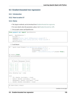
![Learning Apache Spark with Python
(continued from previous page)
+-------+-----------------+------------------+------------------+-------------
˓
→-----+
|summary| TV| Radio| Newspaper|
˓
→Sales|
+-------+-----------------+------------------+------------------+-------------
˓
→-----+
| count| 200| 200| 200|
˓
→ 200|
| mean| 147.0425|23.264000000000024|30.553999999999995|14.
˓
→022500000000003|
| stddev|85.85423631490805|14.846809176168728| 21.77862083852283| 5.
˓
→217456565710477|
| min| 0.7| 0.0| 0.3|
˓
→ 1.6|
| max| 296.4| 49.6| 114.0|
˓
→ 27.0|
+-------+-----------------+------------------+------------------+-------------
˓
→-----+
3. Convert the data to dense vector (features and label)
Note:
You are strongly encouraged to try my get_dummy function for dealing with the categorical
data in comple dataset.
Supervised learning version:
def get_dummy(df,indexCol,categoricalCols,continuousCols,
˓
→labelCol):
from pyspark.ml import Pipeline
from pyspark.ml.feature import StringIndexer,
˓
→OneHotEncoder, VectorAssembler
from pyspark.sql.functions import col
indexers = [ StringIndexer(inputCol=c, outputCol="{0}_
˓
→indexed".format(c))
for c in categoricalCols ]
# default setting: dropLast=True
encoders = [ OneHotEncoder(inputCol=indexer.
˓
→getOutputCol(),
outputCol="{0}_encoded".format(indexer.
˓
→getOutputCol()))
for indexer in indexers ]
assembler = VectorAssembler(inputCols=[encoder.
˓
→getOutputCol() for encoder in encoders]
+ continuousCols, outputCol=
˓
→"features")
(continues on next page)
160 Chapter 9. Regression](https://image.slidesharecdn.com/pyspark-230429134708-b35c8a19/85/pyspark-pdf-166-320.jpg)
![Learning Apache Spark with Python
(continued from previous page)
pipeline = Pipeline(stages=indexers + encoders +
˓
→[assembler])
model=pipeline.fit(df)
data = model.transform(df)
data = data.withColumn('label',col(labelCol))
return data.select(indexCol,'features','label')
Unsupervised learning version:
def get_dummy(df,indexCol,categoricalCols,continuousCols):
'''
Get dummy variables and concat with continuous variables
˓
→for unsupervised learning.
:param df: the dataframe
:param categoricalCols: the name list of the categorical
˓
→data
:param continuousCols: the name list of the numerical
˓
→data
:return k: feature matrix
:author: Wenqiang Feng
:email: von198@gmail.com
'''
indexers = [ StringIndexer(inputCol=c, outputCol="{0}_
˓
→indexed".format(c))
for c in categoricalCols ]
# default setting: dropLast=True
encoders = [ OneHotEncoder(inputCol=indexer.
˓
→getOutputCol(),
outputCol="{0}_encoded".format(indexer.
˓
→getOutputCol()))
for indexer in indexers ]
assembler = VectorAssembler(inputCols=[encoder.
˓
→getOutputCol() for encoder in encoders]
+ continuousCols, outputCol=
˓
→"features")
pipeline = Pipeline(stages=indexers + encoders +
˓
→[assembler])
model=pipeline.fit(df)
data = model.transform(df)
return data.select(indexCol,'features')
9.5. Gradient-boosted tree regression 161](https://image.slidesharecdn.com/pyspark-230429134708-b35c8a19/85/pyspark-pdf-167-320.jpg)
![Learning Apache Spark with Python
Two in one:
def get_dummy(df,indexCol,categoricalCols,continuousCols,labelCol,
˓
→dropLast=False):
'''
Get dummy variables and concat with continuous variables for ml
˓
→modeling.
:param df: the dataframe
:param categoricalCols: the name list of the categorical data
:param continuousCols: the name list of the numerical data
:param labelCol: the name of label column
:param dropLast: the flag of drop last column
:return: feature matrix
:author: Wenqiang Feng
:email: von198@gmail.com
>>> df = spark.createDataFrame([
(0, "a"),
(1, "b"),
(2, "c"),
(3, "a"),
(4, "a"),
(5, "c")
], ["id", "category"])
>>> indexCol = 'id'
>>> categoricalCols = ['category']
>>> continuousCols = []
>>> labelCol = []
>>> mat = get_dummy(df,indexCol,categoricalCols,continuousCols,
˓
→labelCol)
>>> mat.show()
>>>
+---+-------------+
| id| features|
+---+-------------+
| 0|[1.0,0.0,0.0]|
| 1|[0.0,0.0,1.0]|
| 2|[0.0,1.0,0.0]|
| 3|[1.0,0.0,0.0]|
| 4|[1.0,0.0,0.0]|
| 5|[0.0,1.0,0.0]|
+---+-------------+
'''
from pyspark.ml import Pipeline
from pyspark.ml.feature import StringIndexer, OneHotEncoder,
˓
→VectorAssembler
from pyspark.sql.functions import col
(continues on next page)
162 Chapter 9. Regression](https://image.slidesharecdn.com/pyspark-230429134708-b35c8a19/85/pyspark-pdf-168-320.jpg)
![Learning Apache Spark with Python
(continued from previous page)
indexers = [ StringIndexer(inputCol=c, outputCol="{0}_indexed".
˓
→format(c))
for c in categoricalCols ]
# default setting: dropLast=True
encoders = [ OneHotEncoder(inputCol=indexer.getOutputCol(),
outputCol="{0}_encoded".format(indexer.
˓
→getOutputCol()),dropLast=dropLast)
for indexer in indexers ]
assembler = VectorAssembler(inputCols=[encoder.getOutputCol()
˓
→for encoder in encoders]
+ continuousCols, outputCol="features
˓
→")
pipeline = Pipeline(stages=indexers + encoders + [assembler])
model=pipeline.fit(df)
data = model.transform(df)
if indexCol and labelCol:
# for supervised learning
data = data.withColumn('label',col(labelCol))
return data.select(indexCol,'features','label')
elif not indexCol and labelCol:
# for supervised learning
data = data.withColumn('label',col(labelCol))
return data.select('features','label')
elif indexCol and not labelCol:
# for unsupervised learning
return data.select(indexCol,'features')
elif not indexCol and not labelCol:
# for unsupervised learning
return data.select('features')
from pyspark.sql import Row
from pyspark.ml.linalg import Vectors
# convert the data to dense vector
#def transData(row):
# return Row(label=row["Sales"],
# features=Vectors.dense([row["TV"],
# row["Radio"],
# row["Newspaper"]]))
def transData(data):
return data.rdd.map(lambda r: [Vectors.dense(r[:-1]),r[-1]]).toDF([
˓
→'features','label'])
4. Convert the data to dense vector
9.5. Gradient-boosted tree regression 163](https://image.slidesharecdn.com/pyspark-230429134708-b35c8a19/85/pyspark-pdf-169-320.jpg)
![Learning Apache Spark with Python
transformed= transData(df)
transformed.show(5)
+-----------------+-----+
| features|label|
+-----------------+-----+
|[230.1,37.8,69.2]| 22.1|
| [44.5,39.3,45.1]| 10.4|
| [17.2,45.9,69.3]| 9.3|
|[151.5,41.3,58.5]| 18.5|
|[180.8,10.8,58.4]| 12.9|
+-----------------+-----+
only showing top 5 rows
5. Deal with the Categorical variables
from pyspark.ml import Pipeline
from pyspark.ml.regression import GBTRegressor
from pyspark.ml.feature import VectorIndexer
from pyspark.ml.evaluation import RegressionEvaluator
featureIndexer = VectorIndexer(inputCol="features",
outputCol="indexedFeatures",
maxCategories=4).fit(transformed)
data = featureIndexer.transform(transformed)
data.show(5,True)
+-----------------+-----+-----------------+
| features|label| indexedFeatures|
+-----------------+-----+-----------------+
|[230.1,37.8,69.2]| 22.1|[230.1,37.8,69.2]|
| [44.5,39.3,45.1]| 10.4| [44.5,39.3,45.1]|
| [17.2,45.9,69.3]| 9.3| [17.2,45.9,69.3]|
|[151.5,41.3,58.5]| 18.5|[151.5,41.3,58.5]|
|[180.8,10.8,58.4]| 12.9|[180.8,10.8,58.4]|
+-----------------+-----+-----------------+
only showing top 5 rows
6. Split the data into training and test sets (40% held out for testing)
# Split the data into training and test sets (40% held out for testing)
(trainingData, testData) = data.randomSplit([0.6, 0.4])
trainingData.show(5)
testData.show(5)
+----------------+-----+----------------+
| features|label| indexedFeatures|
+----------------+-----+----------------+
| [0.7,39.6,8.7]| 1.6| [0.7,39.6,8.7]|
(continues on next page)
164 Chapter 9. Regression](https://image.slidesharecdn.com/pyspark-230429134708-b35c8a19/85/pyspark-pdf-170-320.jpg)
![Learning Apache Spark with Python
(continued from previous page)
| [8.6,2.1,1.0]| 4.8| [8.6,2.1,1.0]|
| [8.7,48.9,75.0]| 7.2| [8.7,48.9,75.0]|
|[11.7,36.9,45.2]| 7.3|[11.7,36.9,45.2]|
|[13.2,15.9,49.6]| 5.6|[13.2,15.9,49.6]|
+----------------+-----+----------------+
only showing top 5 rows
+---------------+-----+---------------+
| features|label|indexedFeatures|
+---------------+-----+---------------+
| [4.1,11.6,5.7]| 3.2| [4.1,11.6,5.7]|
| [5.4,29.9,9.4]| 5.3| [5.4,29.9,9.4]|
|[7.3,28.1,41.4]| 5.5|[7.3,28.1,41.4]|
|[7.8,38.9,50.6]| 6.6|[7.8,38.9,50.6]|
| [8.4,27.2,2.1]| 5.7| [8.4,27.2,2.1]|
+---------------+-----+---------------+
only showing top 5 rows
7. Fit RandomForest Regression Model
# Import LinearRegression class
from pyspark.ml.regression import GBTRegressor
# Define LinearRegression algorithm
rf = GBTRegressor() #numTrees=2, maxDepth=2, seed=42
Note: If you decide to use the indexedFeatures features, you need to add the parameter
featuresCol="indexedFeatures".
8. Pipeline Architecture
# Chain indexer and tree in a Pipeline
pipeline = Pipeline(stages=[featureIndexer, rf])
model = pipeline.fit(trainingData)
9. Make predictions
predictions = model.transform(testData)
# Select example rows to display.
predictions.select("features","label", "prediction").show(5)
+----------------+-----+------------------+
| features|label| prediction|
+----------------+-----+------------------+
| [7.8,38.9,50.6]| 6.6| 6.836040343319862|
| [8.6,2.1,1.0]| 4.8| 5.652202764688849|
| [8.7,48.9,75.0]| 7.2| 6.908750296855572|
| [13.1,0.4,25.6]| 5.3| 5.784020210692574|
(continues on next page)
9.5. Gradient-boosted tree regression 165](https://image.slidesharecdn.com/pyspark-230429134708-b35c8a19/85/pyspark-pdf-171-320.jpg)
![Learning Apache Spark with Python
(continued from previous page)
|[19.6,20.1,17.0]| 7.6|6.8678921062629295|
+----------------+-----+------------------+
only showing top 5 rows
10. Evaluation
# Select (prediction, true label) and compute test error
evaluator = RegressionEvaluator(
labelCol="label", predictionCol="prediction", metricName="rmse")
rmse = evaluator.evaluate(predictions)
print("Root Mean Squared Error (RMSE) on test data = %g" % rmse)
Root Mean Squared Error (RMSE) on test data = 1.36939
import sklearn.metrics
r2_score = sklearn.metrics.r2_score(y_true, y_pred)
print('r2_score: {:4.3f}'.format(r2_score))
r2_score: 0.932
11. Feature importances
model.stages[-1].featureImportances
SparseVector(3, {0: 0.3716, 1: 0.3525, 2: 0.2759})
model.stages[-1].trees
[DecisionTreeRegressionModel (uid=dtr_7f5cd2ef7cb6) of depth 5 with 61 nodes,
DecisionTreeRegressionModel (uid=dtr_ef3ab6baeac9) of depth 5 with 39 nodes,
DecisionTreeRegressionModel (uid=dtr_07c6e3cf3819) of depth 5 with 45 nodes,
DecisionTreeRegressionModel (uid=dtr_ce724af79a2b) of depth 5 with 47 nodes,
DecisionTreeRegressionModel (uid=dtr_d149ecc71658) of depth 5 with 55 nodes,
DecisionTreeRegressionModel (uid=dtr_d3a79bdea516) of depth 5 with 43 nodes,
DecisionTreeRegressionModel (uid=dtr_7abc1a337844) of depth 5 with 51 nodes,
DecisionTreeRegressionModel (uid=dtr_480834b46d8f) of depth 5 with 33 nodes,
DecisionTreeRegressionModel (uid=dtr_0cbd1eaa3874) of depth 5 with 39 nodes,
DecisionTreeRegressionModel (uid=dtr_8088ac71a204) of depth 5 with 57 nodes,
DecisionTreeRegressionModel (uid=dtr_2ceb9e8deb45) of depth 5 with 47 nodes,
DecisionTreeRegressionModel (uid=dtr_cc334e84e9a2) of depth 5 with 57 nodes,
DecisionTreeRegressionModel (uid=dtr_a665c562929e) of depth 5 with 41 nodes,
DecisionTreeRegressionModel (uid=dtr_2999b1ffd2dc) of depth 5 with 45 nodes,
DecisionTreeRegressionModel (uid=dtr_29965cbe8cfc) of depth 5 with 55 nodes,
DecisionTreeRegressionModel (uid=dtr_731df51bf0ad) of depth 5 with 41 nodes,
DecisionTreeRegressionModel (uid=dtr_354cf33424da) of depth 5 with 51 nodes,
DecisionTreeRegressionModel (uid=dtr_4230f200b1c0) of depth 5 with 41 nodes,
DecisionTreeRegressionModel (uid=dtr_3279cdc1ce1d) of depth 5 with 45 nodes,
DecisionTreeRegressionModel (uid=dtr_f474a99ff06e) of depth 5 with 55 nodes]
166 Chapter 9. Regression](https://image.slidesharecdn.com/pyspark-230429134708-b35c8a19/85/pyspark-pdf-172-320.jpg)
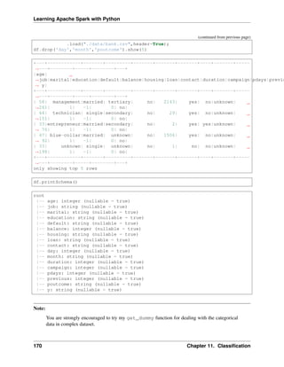
![Learning Apache Spark with Python
Supervised learning version:
def get_dummy(df,indexCol,categoricalCols,continuousCols,
˓
→labelCol):
from pyspark.ml import Pipeline
from pyspark.ml.feature import StringIndexer,
˓
→OneHotEncoder, VectorAssembler
from pyspark.sql.functions import col
indexers = [ StringIndexer(inputCol=c, outputCol="{0}_
˓
→indexed".format(c))
for c in categoricalCols ]
# default setting: dropLast=True
encoders = [ OneHotEncoder(inputCol=indexer.
˓
→getOutputCol(),
outputCol="{0}_encoded".format(indexer.
˓
→getOutputCol()))
for indexer in indexers ]
assembler = VectorAssembler(inputCols=[encoder.
˓
→getOutputCol() for encoder in encoders]
+ continuousCols, outputCol=
˓
→"features")
pipeline = Pipeline(stages=indexers + encoders +
˓
→[assembler])
model=pipeline.fit(df)
data = model.transform(df)
data = data.withColumn('label',col(labelCol))
return data.select(indexCol,'features','label')
Unsupervised learning version:
def get_dummy(df,indexCol,categoricalCols,continuousCols):
'''
Get dummy variables and concat with continuous variables
˓
→for unsupervised learning.
:param df: the dataframe
:param categoricalCols: the name list of the categorical
˓
→data
:param continuousCols: the name list of the numerical
˓
→data
:return k: feature matrix
:author: Wenqiang Feng
:email: von198@gmail.com
'''
(continues on next page)
11.1. Binomial logistic regression 171](https://image.slidesharecdn.com/pyspark-230429134708-b35c8a19/85/pyspark-pdf-177-320.jpg)
![Learning Apache Spark with Python
(continued from previous page)
indexers = [ StringIndexer(inputCol=c, outputCol="{0}_
˓
→indexed".format(c))
for c in categoricalCols ]
# default setting: dropLast=True
encoders = [ OneHotEncoder(inputCol=indexer.
˓
→getOutputCol(),
outputCol="{0}_encoded".format(indexer.
˓
→getOutputCol()))
for indexer in indexers ]
assembler = VectorAssembler(inputCols=[encoder.
˓
→getOutputCol() for encoder in encoders]
+ continuousCols, outputCol=
˓
→"features")
pipeline = Pipeline(stages=indexers + encoders +
˓
→[assembler])
model=pipeline.fit(df)
data = model.transform(df)
return data.select(indexCol,'features')
Two in one:
def get_dummy(df,indexCol,categoricalCols,continuousCols,labelCol,
˓
→dropLast=False):
'''
Get dummy variables and concat with continuous variables for ml
˓
→modeling.
:param df: the dataframe
:param categoricalCols: the name list of the categorical data
:param continuousCols: the name list of the numerical data
:param labelCol: the name of label column
:param dropLast: the flag of drop last column
:return: feature matrix
:author: Wenqiang Feng
:email: von198@gmail.com
>>> df = spark.createDataFrame([
(0, "a"),
(1, "b"),
(2, "c"),
(3, "a"),
(4, "a"),
(5, "c")
], ["id", "category"])
>>> indexCol = 'id'
(continues on next page)
172 Chapter 11. Classification](https://image.slidesharecdn.com/pyspark-230429134708-b35c8a19/85/pyspark-pdf-178-320.jpg)
![Learning Apache Spark with Python
(continued from previous page)
>>> categoricalCols = ['category']
>>> continuousCols = []
>>> labelCol = []
>>> mat = get_dummy(df,indexCol,categoricalCols,continuousCols,
˓
→labelCol)
>>> mat.show()
>>>
+---+-------------+
| id| features|
+---+-------------+
| 0|[1.0,0.0,0.0]|
| 1|[0.0,0.0,1.0]|
| 2|[0.0,1.0,0.0]|
| 3|[1.0,0.0,0.0]|
| 4|[1.0,0.0,0.0]|
| 5|[0.0,1.0,0.0]|
+---+-------------+
'''
from pyspark.ml import Pipeline
from pyspark.ml.feature import StringIndexer, OneHotEncoder,
˓
→VectorAssembler
from pyspark.sql.functions import col
indexers = [ StringIndexer(inputCol=c, outputCol="{0}_indexed".
˓
→format(c))
for c in categoricalCols ]
# default setting: dropLast=True
encoders = [ OneHotEncoder(inputCol=indexer.getOutputCol(),
outputCol="{0}_encoded".format(indexer.
˓
→getOutputCol()),dropLast=dropLast)
for indexer in indexers ]
assembler = VectorAssembler(inputCols=[encoder.getOutputCol()
˓
→for encoder in encoders]
+ continuousCols, outputCol="features
˓
→")
pipeline = Pipeline(stages=indexers + encoders + [assembler])
model=pipeline.fit(df)
data = model.transform(df)
if indexCol and labelCol:
# for supervised learning
data = data.withColumn('label',col(labelCol))
return data.select(indexCol,'features','label')
elif not indexCol and labelCol:
# for supervised learning
(continues on next page)
11.1. Binomial logistic regression 173](https://image.slidesharecdn.com/pyspark-230429134708-b35c8a19/85/pyspark-pdf-179-320.jpg)
![Learning Apache Spark with Python
(continued from previous page)
data = data.withColumn('label',col(labelCol))
return data.select('features','label')
elif indexCol and not labelCol:
# for unsupervised learning
return data.select(indexCol,'features')
elif not indexCol and not labelCol:
# for unsupervised learning
return data.select('features')
def get_dummy(df,categoricalCols,continuousCols,labelCol):
from pyspark.ml import Pipeline
from pyspark.ml.feature import StringIndexer, OneHotEncoder,
˓
→VectorAssembler
from pyspark.sql.functions import col
indexers = [ StringIndexer(inputCol=c, outputCol="{0}_indexed".format(c))
for c in categoricalCols ]
# default setting: dropLast=True
encoders = [ OneHotEncoder(inputCol=indexer.getOutputCol(),
outputCol="{0}_encoded".format(indexer.getOutputCol()))
for indexer in indexers ]
assembler = VectorAssembler(inputCols=[encoder.getOutputCol() for encoder
˓
→in encoders]
+ continuousCols, outputCol="features")
pipeline = Pipeline(stages=indexers + encoders + [assembler])
model=pipeline.fit(df)
data = model.transform(df)
data = data.withColumn('label',col(labelCol))
return data.select('features','label')
3. Deal with categorical data and Convert the data to dense vector
catcols = ['job','marital','education','default',
'housing','loan','contact','poutcome']
num_cols = ['balance', 'duration','campaign','pdays','previous',]
labelCol = 'y'
data = get_dummy(df,catcols,num_cols,labelCol)
data.show(5)
+--------------------+-----+
| features|label|
(continues on next page)
174 Chapter 11. Classification](https://image.slidesharecdn.com/pyspark-230429134708-b35c8a19/85/pyspark-pdf-180-320.jpg)
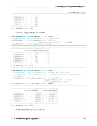
![Learning Apache Spark with Python
# Split the data into training and test sets (40% held out for testing)
(trainingData, testData) = data.randomSplit([0.6, 0.4])
trainingData.show(5,False)
testData.show(5,False)
+-----------------------------------------------------------------------------
˓
→--------------------+-----+
|features
˓
→ |label|
+-----------------------------------------------------------------------------
˓
→--------------------+-----+
|(29,[0,11,13,16,17,18,19,21,24,25,26,27],[1.0,1.0,1.0,1.0,1.0,1.0,1.0,1.0,-
˓
→731.0,401.0,4.0,-1.0])|no |
|(29,[0,11,13,16,17,18,19,21,24,25,26,27],[1.0,1.0,1.0,1.0,1.0,1.0,1.0,1.0,-
˓
→723.0,112.0,2.0,-1.0])|no |
|(29,[0,11,13,16,17,18,19,21,24,25,26,27],[1.0,1.0,1.0,1.0,1.0,1.0,1.0,1.0,-
˓
→626.0,205.0,1.0,-1.0])|no |
|(29,[0,11,13,16,17,18,19,21,24,25,26,27],[1.0,1.0,1.0,1.0,1.0,1.0,1.0,1.0,-
˓
→498.0,357.0,1.0,-1.0])|no |
|(29,[0,11,13,16,17,18,19,21,24,25,26,27],[1.0,1.0,1.0,1.0,1.0,1.0,1.0,1.0,-
˓
→477.0,473.0,2.0,-1.0])|no |
+-----------------------------------------------------------------------------
˓
→--------------------+-----+
only showing top 5 rows
+-----------------------------------------------------------------------------
˓
→--------------------+-----+
|features
˓
→ |label|
+-----------------------------------------------------------------------------
˓
→--------------------+-----+
|(29,[0,11,13,16,17,18,19,21,24,25,26,27],[1.0,1.0,1.0,1.0,1.0,1.0,1.0,1.0,-
˓
→648.0,280.0,2.0,-1.0])|no |
|(29,[0,11,13,16,17,18,19,21,24,25,26,27],[1.0,1.0,1.0,1.0,1.0,1.0,1.0,1.0,-
˓
→596.0,147.0,1.0,-1.0])|no |
|(29,[0,11,13,16,17,18,19,21,24,25,26,27],[1.0,1.0,1.0,1.0,1.0,1.0,1.0,1.0,-
˓
→529.0,416.0,4.0,-1.0])|no |
|(29,[0,11,13,16,17,18,19,21,24,25,26,27],[1.0,1.0,1.0,1.0,1.0,1.0,1.0,1.0,-
˓
→518.0,46.0,5.0,-1.0]) |no |
|(29,[0,11,13,16,17,18,19,21,24,25,26,27],[1.0,1.0,1.0,1.0,1.0,1.0,1.0,1.0,-
˓
→470.0,275.0,2.0,-1.0])|no |
+-----------------------------------------------------------------------------
˓
→--------------------+-----+
only showing top 5 rows
6. Fit Logistic Regression Model
from pyspark.ml.classification import LogisticRegression
logr = LogisticRegression(featuresCol='indexedFeatures', labelCol=
˓
→'indexedLabel')
7. Pipeline Architecture
176 Chapter 11. Classification](https://image.slidesharecdn.com/pyspark-230429134708-b35c8a19/85/pyspark-pdf-182-320.jpg)
![Learning Apache Spark with Python
# Convert indexed labels back to original labels.
labelConverter = IndexToString(inputCol="prediction", outputCol=
˓
→"predictedLabel",
labels=labelIndexer.labels)
# Chain indexers and tree in a Pipeline
pipeline = Pipeline(stages=[labelIndexer, featureIndexer, logr,
˓
→labelConverter])
# Train model. This also runs the indexers.
model = pipeline.fit(trainingData)
8. Make predictions
# Make predictions.
predictions = model.transform(testData)
# Select example rows to display.
predictions.select("features","label","predictedLabel").show(5)
+--------------------+-----+--------------+
| features|label|predictedLabel|
+--------------------+-----+--------------+
|(29,[0,11,13,16,1...| no| no|
|(29,[0,11,13,16,1...| no| no|
|(29,[0,11,13,16,1...| no| no|
|(29,[0,11,13,16,1...| no| no|
|(29,[0,11,13,16,1...| no| no|
+--------------------+-----+--------------+
only showing top 5 rows
9. Evaluation
from pyspark.ml.evaluation import MulticlassClassificationEvaluator
# Select (prediction, true label) and compute test error
evaluator = MulticlassClassificationEvaluator(
labelCol="indexedLabel", predictionCol="prediction", metricName="accuracy
˓
→")
accuracy = evaluator.evaluate(predictions)
print("Test Error = %g" % (1.0 - accuracy))
Test Error = 0.0987688
lrModel = model.stages[2]
trainingSummary = lrModel.summary
# Obtain the objective per iteration
# objectiveHistory = trainingSummary.objectiveHistory
# print("objectiveHistory:")
# for objective in objectiveHistory:
(continues on next page)
11.1. Binomial logistic regression 177](https://image.slidesharecdn.com/pyspark-230429134708-b35c8a19/85/pyspark-pdf-183-320.jpg)
![Learning Apache Spark with Python
(continued from previous page)
# print(objective)
# Obtain the receiver-operating characteristic as a dataframe and
˓
→areaUnderROC.
trainingSummary.roc.show(5)
print("areaUnderROC: " + str(trainingSummary.areaUnderROC))
# Set the model threshold to maximize F-Measure
fMeasure = trainingSummary.fMeasureByThreshold
maxFMeasure = fMeasure.groupBy().max('F-Measure').select('max(F-Measure)').
˓
→head(5)
# bestThreshold = fMeasure.where(fMeasure['F-Measure'] == maxFMeasure['max(F-
˓
→Measure)'])
# .select('threshold').head()['threshold']
# lr.setThreshold(bestThreshold)
You can use z.show() to get the data and plot the ROC curves:
You can also register a TempTable data.registerTempTable('roc_data') and then use sql to
plot the ROC curve:
178 Chapter 11. Classification](https://image.slidesharecdn.com/pyspark-230429134708-b35c8a19/85/pyspark-pdf-184-320.jpg)
![Learning Apache Spark with Python
10. visualization
import matplotlib.pyplot as plt
import numpy as np
import itertools
def plot_confusion_matrix(cm, classes,
normalize=False,
title='Confusion matrix',
cmap=plt.cm.Blues):
"""
This function prints and plots the confusion matrix.
Normalization can be applied by setting `normalize=True`.
"""
if normalize:
cm = cm.astype('float') / cm.sum(axis=1)[:, np.newaxis]
print("Normalized confusion matrix")
else:
print('Confusion matrix, without normalization')
print(cm)
plt.imshow(cm, interpolation='nearest', cmap=cmap)
plt.title(title)
plt.colorbar()
tick_marks = np.arange(len(classes))
plt.xticks(tick_marks, classes, rotation=45)
plt.yticks(tick_marks, classes)
fmt = '.2f' if normalize else 'd'
thresh = cm.max() / 2.
for i, j in itertools.product(range(cm.shape[0]), range(cm.shape[1])):
plt.text(j, i, format(cm[i, j], fmt),
horizontalalignment="center",
color="white" if cm[i, j] > thresh else "black")
plt.tight_layout()
plt.ylabel('True label')
plt.xlabel('Predicted label')
class_temp = predictions.select("label").groupBy("label")
.count().sort('count', ascending=False).toPandas()
class_temp = class_temp["label"].values.tolist()
class_names = map(str, class_temp)
# # # print(class_name)
class_names
['no', 'yes']
from sklearn.metrics import confusion_matrix
y_true = predictions.select("label")
y_true = y_true.toPandas()
(continues on next page)
11.1. Binomial logistic regression 179](https://image.slidesharecdn.com/pyspark-230429134708-b35c8a19/85/pyspark-pdf-185-320.jpg)
![Learning Apache Spark with Python
(continued from previous page)
y_pred = predictions.select("predictedLabel")
y_pred = y_pred.toPandas()
cnf_matrix = confusion_matrix(y_true, y_pred,labels=class_names)
cnf_matrix
array([[15657, 379],
[ 1410, 667]])
# Plot non-normalized confusion matrix
plt.figure()
plot_confusion_matrix(cnf_matrix, classes=class_names,
title='Confusion matrix, without normalization')
plt.show()
Confusion matrix, without normalization
[[15657 379]
[ 1410 667]]
# Plot normalized confusion matrix
plt.figure()
plot_confusion_matrix(cnf_matrix, classes=class_names, normalize=True,
title='Normalized confusion matrix')
(continues on next page)
180 Chapter 11. Classification](https://image.slidesharecdn.com/pyspark-230429134708-b35c8a19/85/pyspark-pdf-186-320.jpg)
![Learning Apache Spark with Python
(continued from previous page)
plt.show()
Normalized confusion matrix
[[ 0.97636568 0.02363432]
[ 0.67886375 0.32113625]]
11.2 Multinomial logistic regression
11.2.1 Introduction
11.2.2 Demo
• The Jupyter notebook can be download from Logistic Regression.
• For more details, please visit Logistic Regression API .
Note: In this demo, I introduced a new function get_dummy to deal with the categorical data. I highly
recommend you to use my get_dummy function in the other cases. This function will save a lot of time for
you.
1. Set up spark context and SparkSession
11.2. Multinomial logistic regression 181](https://image.slidesharecdn.com/pyspark-230429134708-b35c8a19/85/pyspark-pdf-187-320.jpg)
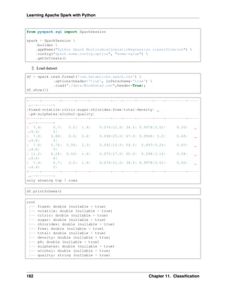
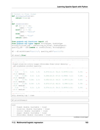
![Learning Apache Spark with Python
(continued from previous page)
|-- free: double (nullable = true)
|-- total: double (nullable = true)
|-- density: double (nullable = true)
|-- pH: double (nullable = true)
|-- sulphates: double (nullable = true)
|-- alcohol: double (nullable = true)
|-- quality: string (nullable = true)
3. Deal with categorical data and Convert the data to dense vector
Note:
You are strongly encouraged to try my get_dummy function for dealing with the categorical
data in complex dataset.
Supervised learning version:
def get_dummy(df,indexCol,categoricalCols,continuousCols,
˓
→labelCol):
from pyspark.ml import Pipeline
from pyspark.ml.feature import StringIndexer,
˓
→OneHotEncoder, VectorAssembler
from pyspark.sql.functions import col
indexers = [ StringIndexer(inputCol=c, outputCol="{0}_
˓
→indexed".format(c))
for c in categoricalCols ]
# default setting: dropLast=True
encoders = [ OneHotEncoder(inputCol=indexer.
˓
→getOutputCol(),
outputCol="{0}_encoded".format(indexer.
˓
→getOutputCol()))
for indexer in indexers ]
assembler = VectorAssembler(inputCols=[encoder.
˓
→getOutputCol() for encoder in encoders]
+ continuousCols, outputCol=
˓
→"features")
pipeline = Pipeline(stages=indexers + encoders +
˓
→[assembler])
model=pipeline.fit(df)
data = model.transform(df)
data = data.withColumn('label',col(labelCol))
return data.select(indexCol,'features','label')
Unsupervised learning version:
184 Chapter 11. Classification](https://image.slidesharecdn.com/pyspark-230429134708-b35c8a19/85/pyspark-pdf-190-320.jpg)
![Learning Apache Spark with Python
def get_dummy(df,indexCol,categoricalCols,continuousCols):
'''
Get dummy variables and concat with continuous variables
˓
→for unsupervised learning.
:param df: the dataframe
:param categoricalCols: the name list of the categorical
˓
→data
:param continuousCols: the name list of the numerical
˓
→data
:return k: feature matrix
:author: Wenqiang Feng
:email: von198@gmail.com
'''
indexers = [ StringIndexer(inputCol=c, outputCol="{0}_
˓
→indexed".format(c))
for c in categoricalCols ]
# default setting: dropLast=True
encoders = [ OneHotEncoder(inputCol=indexer.
˓
→getOutputCol(),
outputCol="{0}_encoded".format(indexer.
˓
→getOutputCol()))
for indexer in indexers ]
assembler = VectorAssembler(inputCols=[encoder.
˓
→getOutputCol() for encoder in encoders]
+ continuousCols, outputCol=
˓
→"features")
pipeline = Pipeline(stages=indexers + encoders +
˓
→[assembler])
model=pipeline.fit(df)
data = model.transform(df)
return data.select(indexCol,'features')
Two in one:
def get_dummy(df,indexCol,categoricalCols,continuousCols,labelCol,
˓
→dropLast=False):
'''
Get dummy variables and concat with continuous variables for ml
˓
→modeling.
:param df: the dataframe
:param categoricalCols: the name list of the categorical data
:param continuousCols: the name list of the numerical data
:param labelCol: the name of label column
:param dropLast: the flag of drop last column
(continues on next page)
11.2. Multinomial logistic regression 185](https://image.slidesharecdn.com/pyspark-230429134708-b35c8a19/85/pyspark-pdf-191-320.jpg)
![Learning Apache Spark with Python
(continued from previous page)
:return: feature matrix
:author: Wenqiang Feng
:email: von198@gmail.com
>>> df = spark.createDataFrame([
(0, "a"),
(1, "b"),
(2, "c"),
(3, "a"),
(4, "a"),
(5, "c")
], ["id", "category"])
>>> indexCol = 'id'
>>> categoricalCols = ['category']
>>> continuousCols = []
>>> labelCol = []
>>> mat = get_dummy(df,indexCol,categoricalCols,continuousCols,
˓
→labelCol)
>>> mat.show()
>>>
+---+-------------+
| id| features|
+---+-------------+
| 0|[1.0,0.0,0.0]|
| 1|[0.0,0.0,1.0]|
| 2|[0.0,1.0,0.0]|
| 3|[1.0,0.0,0.0]|
| 4|[1.0,0.0,0.0]|
| 5|[0.0,1.0,0.0]|
+---+-------------+
'''
from pyspark.ml import Pipeline
from pyspark.ml.feature import StringIndexer, OneHotEncoder,
˓
→VectorAssembler
from pyspark.sql.functions import col
indexers = [ StringIndexer(inputCol=c, outputCol="{0}_indexed".
˓
→format(c))
for c in categoricalCols ]
# default setting: dropLast=True
encoders = [ OneHotEncoder(inputCol=indexer.getOutputCol(),
outputCol="{0}_encoded".format(indexer.
˓
→getOutputCol()),dropLast=dropLast)
for indexer in indexers ]
assembler = VectorAssembler(inputCols=[encoder.getOutputCol()
˓
→for encoder in encoders] (continues on next page)
186 Chapter 11. Classification](https://image.slidesharecdn.com/pyspark-230429134708-b35c8a19/85/pyspark-pdf-192-320.jpg)
![Learning Apache Spark with Python
(continued from previous page)
+ continuousCols, outputCol="features
˓
→")
pipeline = Pipeline(stages=indexers + encoders + [assembler])
model=pipeline.fit(df)
data = model.transform(df)
if indexCol and labelCol:
# for supervised learning
data = data.withColumn('label',col(labelCol))
return data.select(indexCol,'features','label')
elif not indexCol and labelCol:
# for supervised learning
data = data.withColumn('label',col(labelCol))
return data.select('features','label')
elif indexCol and not labelCol:
# for unsupervised learning
return data.select(indexCol,'features')
elif not indexCol and not labelCol:
# for unsupervised learning
return data.select('features')
def get_dummy(df,categoricalCols,continuousCols,labelCol):
from pyspark.ml import Pipeline
from pyspark.ml.feature import StringIndexer, OneHotEncoder,
˓
→VectorAssembler
from pyspark.sql.functions import col
indexers = [ StringIndexer(inputCol=c, outputCol="{0}_indexed".format(c))
for c in categoricalCols ]
# default setting: dropLast=True
encoders = [ OneHotEncoder(inputCol=indexer.getOutputCol(),
outputCol="{0}_encoded".format(indexer.getOutputCol()))
for indexer in indexers ]
assembler = VectorAssembler(inputCols=[encoder.getOutputCol() for encoder
˓
→in encoders]
+ continuousCols, outputCol="features")
pipeline = Pipeline(stages=indexers + encoders + [assembler])
model=pipeline.fit(df)
data = model.transform(df)
data = data.withColumn('label',col(labelCol))
return data.select('features','label')
11.2. Multinomial logistic regression 187](https://image.slidesharecdn.com/pyspark-230429134708-b35c8a19/85/pyspark-pdf-193-320.jpg)
![Learning Apache Spark with Python
4. Transform the dataset to DataFrame
from pyspark.ml.linalg import Vectors # !!!!caution: not from pyspark.mllib.
˓
→linalg import Vectors
from pyspark.ml import Pipeline
from pyspark.ml.feature import IndexToString,StringIndexer, VectorIndexer
from pyspark.ml.tuning import CrossValidator, ParamGridBuilder
from pyspark.ml.evaluation import MulticlassClassificationEvaluator
def transData(data):
return data.rdd.map(lambda r: [Vectors.dense(r[:-1]),r[-1]]).toDF(['features',
˓
→'label'])
transformed = transData(df)
transformed.show(5)
+--------------------+------+
| features| label|
+--------------------+------+
|[7.4,0.7,0.0,1.9,...|medium|
|[7.8,0.88,0.0,2.6...|medium|
|[7.8,0.76,0.04,2....|medium|
|[11.2,0.28,0.56,1...|medium|
|[7.4,0.7,0.0,1.9,...|medium|
+--------------------+------+
only showing top 5 rows
4. Deal with Categorical Label and Variables
# Index labels, adding metadata to the label column
labelIndexer = StringIndexer(inputCol='label',
outputCol='indexedLabel').fit(transformed)
labelIndexer.transform(transformed).show(5, True)
+--------------------+------+------------+
| features| label|indexedLabel|
+--------------------+------+------------+
|[7.4,0.7,0.0,1.9,...|medium| 0.0|
|[7.8,0.88,0.0,2.6...|medium| 0.0|
|[7.8,0.76,0.04,2....|medium| 0.0|
|[11.2,0.28,0.56,1...|medium| 0.0|
|[7.4,0.7,0.0,1.9,...|medium| 0.0|
+--------------------+------+------------+
only showing top 5 rows
# Automatically identify categorical features, and index them.
# Set maxCategories so features with > 4 distinct values are treated as
˓
→continuous.
featureIndexer =VectorIndexer(inputCol="features",
outputCol="indexedFeatures",
maxCategories=4).fit(transformed)
featureIndexer.transform(transformed).show(5, True)
188 Chapter 11. Classification](https://image.slidesharecdn.com/pyspark-230429134708-b35c8a19/85/pyspark-pdf-194-320.jpg)
![Learning Apache Spark with Python
+--------------------+------+--------------------+
| features| label| indexedFeatures|
+--------------------+------+--------------------+
|[7.4,0.7,0.0,1.9,...|medium|[7.4,0.7,0.0,1.9,...|
|[7.8,0.88,0.0,2.6...|medium|[7.8,0.88,0.0,2.6...|
|[7.8,0.76,0.04,2....|medium|[7.8,0.76,0.04,2....|
|[11.2,0.28,0.56,1...|medium|[11.2,0.28,0.56,1...|
|[7.4,0.7,0.0,1.9,...|medium|[7.4,0.7,0.0,1.9,...|
+--------------------+------+--------------------+
only showing top 5 rows
5. Split the data to training and test data sets
# Split the data into training and test sets (40% held out for testing)
(trainingData, testData) = data.randomSplit([0.6, 0.4])
trainingData.show(5,False)
testData.show(5,False)
+---------------------------------------------------------+------+
|features |label |
+---------------------------------------------------------+------+
|[4.7,0.6,0.17,2.3,0.058,17.0,106.0,0.9932,3.85,0.6,12.9] |medium|
|[5.0,0.38,0.01,1.6,0.048,26.0,60.0,0.99084,3.7,0.75,14.0]|medium|
|[5.0,0.4,0.5,4.3,0.046,29.0,80.0,0.9902,3.49,0.66,13.6] |medium|
|[5.0,0.74,0.0,1.2,0.041,16.0,46.0,0.99258,4.01,0.59,12.5]|medium|
|[5.1,0.42,0.0,1.8,0.044,18.0,88.0,0.99157,3.68,0.73,13.6]|high |
+---------------------------------------------------------+------+
only showing top 5 rows
+---------------------------------------------------------+------+
|features |label |
+---------------------------------------------------------+------+
|[4.6,0.52,0.15,2.1,0.054,8.0,65.0,0.9934,3.9,0.56,13.1] |low |
|[4.9,0.42,0.0,2.1,0.048,16.0,42.0,0.99154,3.71,0.74,14.0]|high |
|[5.0,0.42,0.24,2.0,0.06,19.0,50.0,0.9917,3.72,0.74,14.0] |high |
|[5.0,1.02,0.04,1.4,0.045,41.0,85.0,0.9938,3.75,0.48,10.5]|low |
|[5.0,1.04,0.24,1.6,0.05,32.0,96.0,0.9934,3.74,0.62,11.5] |medium|
+---------------------------------------------------------+------+
only showing top 5 rows
6. Fit Multinomial logisticRegression Classification Model
from pyspark.ml.classification import LogisticRegression
logr = LogisticRegression(featuresCol='indexedFeatures', labelCol=
˓
→'indexedLabel')
7. Pipeline Architecture
# Convert indexed labels back to original labels.
labelConverter = IndexToString(inputCol="prediction", outputCol=
˓
→"predictedLabel",
(continues on next page)
11.2. Multinomial logistic regression 189](https://image.slidesharecdn.com/pyspark-230429134708-b35c8a19/85/pyspark-pdf-195-320.jpg)
![Learning Apache Spark with Python
(continued from previous page)
labels=labelIndexer.labels)
# Chain indexers and tree in a Pipeline
pipeline = Pipeline(stages=[labelIndexer, featureIndexer, logr,
˓
→labelConverter])
# Train model. This also runs the indexers.
model = pipeline.fit(trainingData)
8. Make predictions
# Make predictions.
predictions = model.transform(testData)
# Select example rows to display.
predictions.select("features","label","predictedLabel").show(5)
+--------------------+------+--------------+
| features| label|predictedLabel|
+--------------------+------+--------------+
|[4.6,0.52,0.15,2....| low| medium|
|[4.9,0.42,0.0,2.1...| high| high|
|[5.0,0.42,0.24,2....| high| high|
|[5.0,1.02,0.04,1....| low| medium|
|[5.0,1.04,0.24,1....|medium| medium|
+--------------------+------+--------------+
only showing top 5 rows
9. Evaluation
from pyspark.ml.evaluation import MulticlassClassificationEvaluator
# Select (prediction, true label) and compute test error
evaluator = MulticlassClassificationEvaluator(
labelCol="indexedLabel", predictionCol="prediction", metricName="accuracy
˓
→")
accuracy = evaluator.evaluate(predictions)
print("Test Error = %g" % (1.0 - accuracy))
Test Error = 0.181287
lrModel = model.stages[2]
trainingSummary = lrModel.summary
# Obtain the objective per iteration
# objectiveHistory = trainingSummary.objectiveHistory
# print("objectiveHistory:")
# for objective in objectiveHistory:
# print(objective)
(continues on next page)
190 Chapter 11. Classification](https://image.slidesharecdn.com/pyspark-230429134708-b35c8a19/85/pyspark-pdf-196-320.jpg)
![Learning Apache Spark with Python
(continued from previous page)
# Obtain the receiver-operating characteristic as a dataframe and
˓
→areaUnderROC.
trainingSummary.roc.show(5)
print("areaUnderROC: " + str(trainingSummary.areaUnderROC))
# Set the model threshold to maximize F-Measure
fMeasure = trainingSummary.fMeasureByThreshold
maxFMeasure = fMeasure.groupBy().max('F-Measure').select('max(F-Measure)').
˓
→head(5)
# bestThreshold = fMeasure.where(fMeasure['F-Measure'] == maxFMeasure['max(F-
˓
→Measure)'])
# .select('threshold').head()['threshold']
# lr.setThreshold(bestThreshold)
You can use z.show() to get the data and plot the ROC curves:
You can also register a TempTable data.registerTempTable('roc_data') and then use sql to
plot the ROC curve:
10. visualization
11.2. Multinomial logistic regression 191](https://image.slidesharecdn.com/pyspark-230429134708-b35c8a19/85/pyspark-pdf-197-320.jpg)
![Learning Apache Spark with Python
import matplotlib.pyplot as plt
import numpy as np
import itertools
def plot_confusion_matrix(cm, classes,
normalize=False,
title='Confusion matrix',
cmap=plt.cm.Blues):
"""
This function prints and plots the confusion matrix.
Normalization can be applied by setting `normalize=True`.
"""
if normalize:
cm = cm.astype('float') / cm.sum(axis=1)[:, np.newaxis]
print("Normalized confusion matrix")
else:
print('Confusion matrix, without normalization')
print(cm)
plt.imshow(cm, interpolation='nearest', cmap=cmap)
plt.title(title)
plt.colorbar()
tick_marks = np.arange(len(classes))
plt.xticks(tick_marks, classes, rotation=45)
plt.yticks(tick_marks, classes)
fmt = '.2f' if normalize else 'd'
thresh = cm.max() / 2.
for i, j in itertools.product(range(cm.shape[0]), range(cm.shape[1])):
plt.text(j, i, format(cm[i, j], fmt),
horizontalalignment="center",
color="white" if cm[i, j] > thresh else "black")
plt.tight_layout()
plt.ylabel('True label')
plt.xlabel('Predicted label')
class_temp = predictions.select("label").groupBy("label")
.count().sort('count', ascending=False).toPandas()
class_temp = class_temp["label"].values.tolist()
class_names = map(str, class_temp)
# # # print(class_name)
class_names
['medium', 'high', 'low']
from sklearn.metrics import confusion_matrix
y_true = predictions.select("label")
y_true = y_true.toPandas()
(continues on next page)
192 Chapter 11. Classification](https://image.slidesharecdn.com/pyspark-230429134708-b35c8a19/85/pyspark-pdf-198-320.jpg)
![Learning Apache Spark with Python
(continued from previous page)
y_pred = predictions.select("predictedLabel")
y_pred = y_pred.toPandas()
cnf_matrix = confusion_matrix(y_true, y_pred,labels=class_names)
cnf_matrix
array([[526, 11, 2],
[ 73, 33, 0],
[ 38, 0, 1]])
# Plot non-normalized confusion matrix
plt.figure()
plot_confusion_matrix(cnf_matrix, classes=class_names,
title='Confusion matrix, without normalization')
plt.show()
Confusion matrix, without normalization
[[526 11 2]
[ 73 33 0]
[ 38 0 1]]
# Plot normalized confusion matrix
plt.figure()
plot_confusion_matrix(cnf_matrix, classes=class_names, normalize=True,
(continues on next page)
11.2. Multinomial logistic regression 193](https://image.slidesharecdn.com/pyspark-230429134708-b35c8a19/85/pyspark-pdf-199-320.jpg)
![Learning Apache Spark with Python
(continued from previous page)
title='Normalized confusion matrix')
plt.show()
Normalized confusion matrix
[[0.97588126 0.02040816 0.00371058]
[0.68867925 0.31132075 0. ]
[0.97435897 0. 0.02564103]]
11.3 Decision tree Classification
11.3.1 Introduction
11.3.2 Demo
• The Jupyter notebook can be download from Decision Tree Classification.
• For more details, please visit DecisionTreeClassifier API .
1. Set up spark context and SparkSession
from pyspark.sql import SparkSession
(continues on next page)
194 Chapter 11. Classification](https://image.slidesharecdn.com/pyspark-230429134708-b35c8a19/85/pyspark-pdf-200-320.jpg)
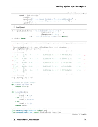
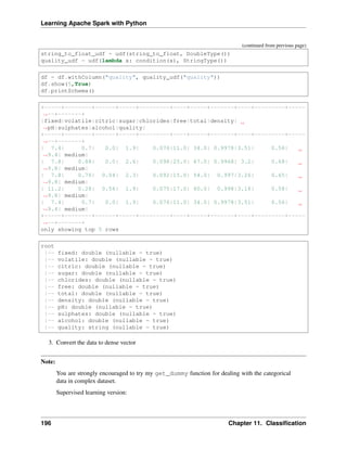
![Learning Apache Spark with Python
def get_dummy(df,indexCol,categoricalCols,continuousCols,
˓
→labelCol):
from pyspark.ml import Pipeline
from pyspark.ml.feature import StringIndexer,
˓
→OneHotEncoder, VectorAssembler
from pyspark.sql.functions import col
indexers = [ StringIndexer(inputCol=c, outputCol="{0}_
˓
→indexed".format(c))
for c in categoricalCols ]
# default setting: dropLast=True
encoders = [ OneHotEncoder(inputCol=indexer.
˓
→getOutputCol(),
outputCol="{0}_encoded".format(indexer.
˓
→getOutputCol()))
for indexer in indexers ]
assembler = VectorAssembler(inputCols=[encoder.
˓
→getOutputCol() for encoder in encoders]
+ continuousCols, outputCol=
˓
→"features")
pipeline = Pipeline(stages=indexers + encoders +
˓
→[assembler])
model=pipeline.fit(df)
data = model.transform(df)
data = data.withColumn('label',col(labelCol))
return data.select(indexCol,'features','label')
Unsupervised learning version:
def get_dummy(df,indexCol,categoricalCols,continuousCols):
'''
Get dummy variables and concat with continuous variables
˓
→for unsupervised learning.
:param df: the dataframe
:param categoricalCols: the name list of the categorical
˓
→data
:param continuousCols: the name list of the numerical
˓
→data
:return k: feature matrix
:author: Wenqiang Feng
:email: von198@gmail.com
'''
indexers = [ StringIndexer(inputCol=c, outputCol="{0}_
˓
→indexed".format(c))
(continues on next page)
11.3. Decision tree Classification 197](https://image.slidesharecdn.com/pyspark-230429134708-b35c8a19/85/pyspark-pdf-203-320.jpg)
![Learning Apache Spark with Python
(continued from previous page)
for c in categoricalCols ]
# default setting: dropLast=True
encoders = [ OneHotEncoder(inputCol=indexer.
˓
→getOutputCol(),
outputCol="{0}_encoded".format(indexer.
˓
→getOutputCol()))
for indexer in indexers ]
assembler = VectorAssembler(inputCols=[encoder.
˓
→getOutputCol() for encoder in encoders]
+ continuousCols, outputCol=
˓
→"features")
pipeline = Pipeline(stages=indexers + encoders +
˓
→[assembler])
model=pipeline.fit(df)
data = model.transform(df)
return data.select(indexCol,'features')
Two in one:
def get_dummy(df,indexCol,categoricalCols,continuousCols,labelCol,
˓
→dropLast=False):
'''
Get dummy variables and concat with continuous variables for ml
˓
→modeling.
:param df: the dataframe
:param categoricalCols: the name list of the categorical data
:param continuousCols: the name list of the numerical data
:param labelCol: the name of label column
:param dropLast: the flag of drop last column
:return: feature matrix
:author: Wenqiang Feng
:email: von198@gmail.com
>>> df = spark.createDataFrame([
(0, "a"),
(1, "b"),
(2, "c"),
(3, "a"),
(4, "a"),
(5, "c")
], ["id", "category"])
>>> indexCol = 'id'
>>> categoricalCols = ['category']
>>> continuousCols = []
(continues on next page)
198 Chapter 11. Classification](https://image.slidesharecdn.com/pyspark-230429134708-b35c8a19/85/pyspark-pdf-204-320.jpg)
![Learning Apache Spark with Python
(continued from previous page)
>>> labelCol = []
>>> mat = get_dummy(df,indexCol,categoricalCols,continuousCols,
˓
→labelCol)
>>> mat.show()
>>>
+---+-------------+
| id| features|
+---+-------------+
| 0|[1.0,0.0,0.0]|
| 1|[0.0,0.0,1.0]|
| 2|[0.0,1.0,0.0]|
| 3|[1.0,0.0,0.0]|
| 4|[1.0,0.0,0.0]|
| 5|[0.0,1.0,0.0]|
+---+-------------+
'''
from pyspark.ml import Pipeline
from pyspark.ml.feature import StringIndexer, OneHotEncoder,
˓
→VectorAssembler
from pyspark.sql.functions import col
indexers = [ StringIndexer(inputCol=c, outputCol="{0}_indexed".
˓
→format(c))
for c in categoricalCols ]
# default setting: dropLast=True
encoders = [ OneHotEncoder(inputCol=indexer.getOutputCol(),
outputCol="{0}_encoded".format(indexer.
˓
→getOutputCol()),dropLast=dropLast)
for indexer in indexers ]
assembler = VectorAssembler(inputCols=[encoder.getOutputCol()
˓
→for encoder in encoders]
+ continuousCols, outputCol="features
˓
→")
pipeline = Pipeline(stages=indexers + encoders + [assembler])
model=pipeline.fit(df)
data = model.transform(df)
if indexCol and labelCol:
# for supervised learning
data = data.withColumn('label',col(labelCol))
return data.select(indexCol,'features','label')
elif not indexCol and labelCol:
# for supervised learning
data = data.withColumn('label',col(labelCol))
return data.select('features','label')
(continues on next page)
11.3. Decision tree Classification 199](https://image.slidesharecdn.com/pyspark-230429134708-b35c8a19/85/pyspark-pdf-205-320.jpg)
![Learning Apache Spark with Python
(continued from previous page)
elif indexCol and not labelCol:
# for unsupervised learning
return data.select(indexCol,'features')
elif not indexCol and not labelCol:
# for unsupervised learning
return data.select('features')
# !!!!caution: not from pyspark.mllib.linalg import Vectors
from pyspark.ml.linalg import Vectors
from pyspark.ml import Pipeline
from pyspark.ml.feature import IndexToString,StringIndexer, VectorIndexer
from pyspark.ml.tuning import CrossValidator, ParamGridBuilder
from pyspark.ml.evaluation import MulticlassClassificationEvaluator
def transData(data):
return data.rdd.map(lambda r: [Vectors.dense(r[:-1]),r[-1]]).toDF([
˓
→'features','label'])
4. Transform the dataset to DataFrame
transformed = transData(df)
transformed.show(5)
+--------------------+------+
| features| label|
+--------------------+------+
|[7.4,0.7,0.0,1.9,...|medium|
|[7.8,0.88,0.0,2.6...|medium|
|[7.8,0.76,0.04,2....|medium|
|[11.2,0.28,0.56,1...|medium|
|[7.4,0.7,0.0,1.9,...|medium|
+--------------------+------+
only showing top 5 rows
5. Deal with Categorical Label and Variables
# Index labels, adding metadata to the label column
labelIndexer = StringIndexer(inputCol='label',
outputCol='indexedLabel').fit(transformed)
labelIndexer.transform(transformed).show(5, True)
+--------------------+------+------------+
| features| label|indexedLabel|
+--------------------+------+------------+
|[7.4,0.7,0.0,1.9,...|medium| 0.0|
|[7.8,0.88,0.0,2.6...|medium| 0.0|
|[7.8,0.76,0.04,2....|medium| 0.0|
|[11.2,0.28,0.56,1...|medium| 0.0|
|[7.4,0.7,0.0,1.9,...|medium| 0.0|
(continues on next page)
200 Chapter 11. Classification](https://image.slidesharecdn.com/pyspark-230429134708-b35c8a19/85/pyspark-pdf-206-320.jpg)
![Learning Apache Spark with Python
(continued from previous page)
+--------------------+------+------------+
only showing top 5 rows
# Automatically identify categorical features, and index them.
# Set maxCategories so features with > 4 distinct values are treated as
˓
→continuous.
featureIndexer =VectorIndexer(inputCol="features",
outputCol="indexedFeatures",
maxCategories=4).fit(transformed)
featureIndexer.transform(transformed).show(5, True)
+--------------------+------+--------------------+
| features| label| indexedFeatures|
+--------------------+------+--------------------+
|[7.4,0.7,0.0,1.9,...|medium|[7.4,0.7,0.0,1.9,...|
|[7.8,0.88,0.0,2.6...|medium|[7.8,0.88,0.0,2.6...|
|[7.8,0.76,0.04,2....|medium|[7.8,0.76,0.04,2....|
|[11.2,0.28,0.56,1...|medium|[11.2,0.28,0.56,1...|
|[7.4,0.7,0.0,1.9,...|medium|[7.4,0.7,0.0,1.9,...|
+--------------------+------+--------------------+
only showing top 5 rows
6. Split the data to training and test data sets
# Split the data into training and test sets (40% held out for testing)
(trainingData, testData) = transformed.randomSplit([0.6, 0.4])
trainingData.show(5)
testData.show(5)
+--------------------+------+
| features| label|
+--------------------+------+
|[4.6,0.52,0.15,2....| low|
|[4.7,0.6,0.17,2.3...|medium|
|[5.0,1.02,0.04,1....| low|
|[5.0,1.04,0.24,1....|medium|
|[5.1,0.585,0.0,1....| high|
+--------------------+------+
only showing top 5 rows
+--------------------+------+
| features| label|
+--------------------+------+
|[4.9,0.42,0.0,2.1...| high|
|[5.0,0.38,0.01,1....|medium|
|[5.0,0.4,0.5,4.3,...|medium|
|[5.0,0.42,0.24,2....| high|
|[5.0,0.74,0.0,1.2...|medium|
+--------------------+------+
only showing top 5 rows
11.3. Decision tree Classification 201](https://image.slidesharecdn.com/pyspark-230429134708-b35c8a19/85/pyspark-pdf-207-320.jpg)
![Learning Apache Spark with Python
7. Fit Decision Tree Classification Model
from pyspark.ml.classification import DecisionTreeClassifier
# Train a DecisionTree model
dTree = DecisionTreeClassifier(labelCol='indexedLabel', featuresCol=
˓
→'indexedFeatures')
8. Pipeline Architecture
# Convert indexed labels back to original labels.
labelConverter = IndexToString(inputCol="prediction", outputCol=
˓
→"predictedLabel",
labels=labelIndexer.labels)
# Chain indexers and tree in a Pipeline
pipeline = Pipeline(stages=[labelIndexer, featureIndexer, dTree,
˓
→labelConverter])
# Train model. This also runs the indexers.
model = pipeline.fit(trainingData)
9. Make predictions
# Make predictions.
predictions = model.transform(testData)
# Select example rows to display.
predictions.select("features","label","predictedLabel").show(5)
+--------------------+------+--------------+
| features| label|predictedLabel|
+--------------------+------+--------------+
|[4.9,0.42,0.0,2.1...| high| high|
|[5.0,0.38,0.01,1....|medium| medium|
|[5.0,0.4,0.5,4.3,...|medium| medium|
|[5.0,0.42,0.24,2....| high| medium|
|[5.0,0.74,0.0,1.2...|medium| medium|
+--------------------+------+--------------+
only showing top 5 rows
10. Evaluation
from pyspark.ml.evaluation import MulticlassClassificationEvaluator
# Select (prediction, true label) and compute test error
evaluator = MulticlassClassificationEvaluator(
labelCol="indexedLabel", predictionCol="prediction", metricName="accuracy
˓
→")
accuracy = evaluator.evaluate(predictions)
print("Test Error = %g" % (1.0 - accuracy))
(continues on next page)
202 Chapter 11. Classification](https://image.slidesharecdn.com/pyspark-230429134708-b35c8a19/85/pyspark-pdf-208-320.jpg)
![Learning Apache Spark with Python
(continued from previous page)
rfModel = model.stages[-2]
print(rfModel) # summary only
Test Error = 0.45509
DecisionTreeClassificationModel (uid=DecisionTreeClassifier_
˓
→4545ac8dca9c8438ef2a)
of depth 5 with 59 nodes
11. visualization
import matplotlib.pyplot as plt
import numpy as np
import itertools
def plot_confusion_matrix(cm, classes,
normalize=False,
title='Confusion matrix',
cmap=plt.cm.Blues):
"""
This function prints and plots the confusion matrix.
Normalization can be applied by setting `normalize=True`.
"""
if normalize:
cm = cm.astype('float') / cm.sum(axis=1)[:, np.newaxis]
print("Normalized confusion matrix")
else:
print('Confusion matrix, without normalization')
print(cm)
plt.imshow(cm, interpolation='nearest', cmap=cmap)
plt.title(title)
plt.colorbar()
tick_marks = np.arange(len(classes))
plt.xticks(tick_marks, classes, rotation=45)
plt.yticks(tick_marks, classes)
fmt = '.2f' if normalize else 'd'
thresh = cm.max() / 2.
for i, j in itertools.product(range(cm.shape[0]), range(cm.shape[1])):
plt.text(j, i, format(cm[i, j], fmt),
horizontalalignment="center",
color="white" if cm[i, j] > thresh else "black")
plt.tight_layout()
plt.ylabel('True label')
plt.xlabel('Predicted label')
class_temp = predictions.select("label").groupBy("label")
.count().sort('count', ascending=False).toPandas()
class_temp = class_temp["label"].values.tolist()
(continues on next page)
11.3. Decision tree Classification 203](https://image.slidesharecdn.com/pyspark-230429134708-b35c8a19/85/pyspark-pdf-209-320.jpg)
![Learning Apache Spark with Python
(continued from previous page)
class_names = map(str, class_temp)
# # # print(class_name)
class_names
['medium', 'high', 'low']
from sklearn.metrics import confusion_matrix
y_true = predictions.select("label")
y_true = y_true.toPandas()
y_pred = predictions.select("predictedLabel")
y_pred = y_pred.toPandas()
cnf_matrix = confusion_matrix(y_true, y_pred,labels=class_names)
cnf_matrix
array([[497, 29, 7],
[ 40, 42, 0],
[ 22, 0, 2]])
# Plot non-normalized confusion matrix
plt.figure()
plot_confusion_matrix(cnf_matrix, classes=class_names,
title='Confusion matrix, without normalization')
plt.show()
Confusion matrix, without normalization
[[497 29 7]
[ 40 42 0]
[ 22 0 2]]
204 Chapter 11. Classification](https://image.slidesharecdn.com/pyspark-230429134708-b35c8a19/85/pyspark-pdf-210-320.jpg)
![Learning Apache Spark with Python
# Plot normalized confusion matrix
plt.figure()
plot_confusion_matrix(cnf_matrix, classes=class_names, normalize=True,
title='Normalized confusion matrix')
plt.show()
Normalized confusion matrix
[[ 0.93245779 0.05440901 0.01313321]
[ 0.48780488 0.51219512 0. ]
[ 0.91666667 0. 0.08333333]]
11.3. Decision tree Classification 205](https://image.slidesharecdn.com/pyspark-230429134708-b35c8a19/85/pyspark-pdf-211-320.jpg)
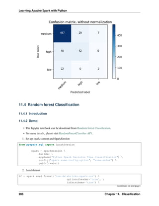
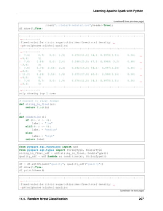
![Learning Apache Spark with Python
(continued from previous page)
+-----+--------+------+-----+---------+----+-----+-------+----+---------+-----
˓
→--+-------+
| 7.4| 0.7| 0.0| 1.9| 0.076|11.0| 34.0| 0.9978|3.51| 0.56|
˓
→9.4| medium|
| 7.8| 0.88| 0.0| 2.6| 0.098|25.0| 67.0| 0.9968| 3.2| 0.68|
˓
→9.8| medium|
| 7.8| 0.76| 0.04| 2.3| 0.092|15.0| 54.0| 0.997|3.26| 0.65|
˓
→9.8| medium|
| 11.2| 0.28| 0.56| 1.9| 0.075|17.0| 60.0| 0.998|3.16| 0.58|
˓
→9.8| medium|
| 7.4| 0.7| 0.0| 1.9| 0.076|11.0| 34.0| 0.9978|3.51| 0.56|
˓
→9.4| medium|
+-----+--------+------+-----+---------+----+-----+-------+----+---------+-----
˓
→--+-------+
only showing top 5 rows
root
|-- fixed: double (nullable = true)
|-- volatile: double (nullable = true)
|-- citric: double (nullable = true)
|-- sugar: double (nullable = true)
|-- chlorides: double (nullable = true)
|-- free: double (nullable = true)
|-- total: double (nullable = true)
|-- density: double (nullable = true)
|-- pH: double (nullable = true)
|-- sulphates: double (nullable = true)
|-- alcohol: double (nullable = true)
|-- quality: string (nullable = true)
3. Convert the data to dense vector
Note:
You are strongly encouraged to try my get_dummy function for dealing with the categorical
data in complex dataset.
Supervised learning version:
def get_dummy(df,indexCol,categoricalCols,continuousCols,
˓
→labelCol):
from pyspark.ml import Pipeline
from pyspark.ml.feature import StringIndexer,
˓
→OneHotEncoder, VectorAssembler
from pyspark.sql.functions import col
indexers = [ StringIndexer(inputCol=c, outputCol="{0}_
˓
→indexed".format(c))
for c in categoricalCols ]
(continues on next page)
208 Chapter 11. Classification](https://image.slidesharecdn.com/pyspark-230429134708-b35c8a19/85/pyspark-pdf-214-320.jpg)
![Learning Apache Spark with Python
(continued from previous page)
# default setting: dropLast=True
encoders = [ OneHotEncoder(inputCol=indexer.
˓
→getOutputCol(),
outputCol="{0}_encoded".format(indexer.
˓
→getOutputCol()))
for indexer in indexers ]
assembler = VectorAssembler(inputCols=[encoder.
˓
→getOutputCol() for encoder in encoders]
+ continuousCols, outputCol=
˓
→"features")
pipeline = Pipeline(stages=indexers + encoders +
˓
→[assembler])
model=pipeline.fit(df)
data = model.transform(df)
data = data.withColumn('label',col(labelCol))
return data.select(indexCol,'features','label')
Unsupervised learning version:
def get_dummy(df,indexCol,categoricalCols,continuousCols):
'''
Get dummy variables and concat with continuous variables
˓
→for unsupervised learning.
:param df: the dataframe
:param categoricalCols: the name list of the categorical
˓
→data
:param continuousCols: the name list of the numerical
˓
→data
:return k: feature matrix
:author: Wenqiang Feng
:email: von198@gmail.com
'''
indexers = [ StringIndexer(inputCol=c, outputCol="{0}_
˓
→indexed".format(c))
for c in categoricalCols ]
# default setting: dropLast=True
encoders = [ OneHotEncoder(inputCol=indexer.
˓
→getOutputCol(),
outputCol="{0}_encoded".format(indexer.
˓
→getOutputCol()))
for indexer in indexers ]
assembler = VectorAssembler(inputCols=[encoder.
˓
→getOutputCol() for encoder in encoders]
(continues on next page)
11.4. Random forest Classification 209](https://image.slidesharecdn.com/pyspark-230429134708-b35c8a19/85/pyspark-pdf-215-320.jpg)
![Learning Apache Spark with Python
(continued from previous page)
+ continuousCols, outputCol=
˓
→"features")
pipeline = Pipeline(stages=indexers + encoders +
˓
→[assembler])
model=pipeline.fit(df)
data = model.transform(df)
return data.select(indexCol,'features')
Two in one:
def get_dummy(df,indexCol,categoricalCols,continuousCols,labelCol,
˓
→dropLast=False):
'''
Get dummy variables and concat with continuous variables for ml
˓
→modeling.
:param df: the dataframe
:param categoricalCols: the name list of the categorical data
:param continuousCols: the name list of the numerical data
:param labelCol: the name of label column
:param dropLast: the flag of drop last column
:return: feature matrix
:author: Wenqiang Feng
:email: von198@gmail.com
>>> df = spark.createDataFrame([
(0, "a"),
(1, "b"),
(2, "c"),
(3, "a"),
(4, "a"),
(5, "c")
], ["id", "category"])
>>> indexCol = 'id'
>>> categoricalCols = ['category']
>>> continuousCols = []
>>> labelCol = []
>>> mat = get_dummy(df,indexCol,categoricalCols,continuousCols,
˓
→labelCol)
>>> mat.show()
>>>
+---+-------------+
| id| features|
+---+-------------+
| 0|[1.0,0.0,0.0]|
(continues on next page)
210 Chapter 11. Classification](https://image.slidesharecdn.com/pyspark-230429134708-b35c8a19/85/pyspark-pdf-216-320.jpg)
![Learning Apache Spark with Python
(continued from previous page)
| 1|[0.0,0.0,1.0]|
| 2|[0.0,1.0,0.0]|
| 3|[1.0,0.0,0.0]|
| 4|[1.0,0.0,0.0]|
| 5|[0.0,1.0,0.0]|
+---+-------------+
'''
from pyspark.ml import Pipeline
from pyspark.ml.feature import StringIndexer, OneHotEncoder,
˓
→VectorAssembler
from pyspark.sql.functions import col
indexers = [ StringIndexer(inputCol=c, outputCol="{0}_indexed".
˓
→format(c))
for c in categoricalCols ]
# default setting: dropLast=True
encoders = [ OneHotEncoder(inputCol=indexer.getOutputCol(),
outputCol="{0}_encoded".format(indexer.
˓
→getOutputCol()),dropLast=dropLast)
for indexer in indexers ]
assembler = VectorAssembler(inputCols=[encoder.getOutputCol()
˓
→for encoder in encoders]
+ continuousCols, outputCol="features
˓
→")
pipeline = Pipeline(stages=indexers + encoders + [assembler])
model=pipeline.fit(df)
data = model.transform(df)
if indexCol and labelCol:
# for supervised learning
data = data.withColumn('label',col(labelCol))
return data.select(indexCol,'features','label')
elif not indexCol and labelCol:
# for supervised learning
data = data.withColumn('label',col(labelCol))
return data.select('features','label')
elif indexCol and not labelCol:
# for unsupervised learning
return data.select(indexCol,'features')
elif not indexCol and not labelCol:
# for unsupervised learning
return data.select('features')
# !!!!caution: not from pyspark.mllib.linalg import Vectors
from pyspark.ml.linalg import Vectors
(continues on next page)
11.4. Random forest Classification 211](https://image.slidesharecdn.com/pyspark-230429134708-b35c8a19/85/pyspark-pdf-217-320.jpg)
![Learning Apache Spark with Python
(continued from previous page)
from pyspark.ml import Pipeline
from pyspark.ml.feature import IndexToString,StringIndexer, VectorIndexer
from pyspark.ml.tuning import CrossValidator, ParamGridBuilder
from pyspark.ml.evaluation import MulticlassClassificationEvaluator
def transData(data):
return data.rdd.map(lambda r: [Vectors.dense(r[:-1]),r[-1]]).toDF([
˓
→'features','label'])
4. Transform the dataset to DataFrame
transformed = transData(df)
transformed.show(5)
+--------------------+------+
| features| label|
+--------------------+------+
|[7.4,0.7,0.0,1.9,...|medium|
|[7.8,0.88,0.0,2.6...|medium|
|[7.8,0.76,0.04,2....|medium|
|[11.2,0.28,0.56,1...|medium|
|[7.4,0.7,0.0,1.9,...|medium|
+--------------------+------+
only showing top 5 rows
5. Deal with Categorical Label and Variables
# Index labels, adding metadata to the label column
labelIndexer = StringIndexer(inputCol='label',
outputCol='indexedLabel').fit(transformed)
labelIndexer.transform(transformed).show(5, True)
+--------------------+------+------------+
| features| label|indexedLabel|
+--------------------+------+------------+
|[7.4,0.7,0.0,1.9,...|medium| 0.0|
|[7.8,0.88,0.0,2.6...|medium| 0.0|
|[7.8,0.76,0.04,2....|medium| 0.0|
|[11.2,0.28,0.56,1...|medium| 0.0|
|[7.4,0.7,0.0,1.9,...|medium| 0.0|
+--------------------+------+------------+
only showing top 5 rows
# Automatically identify categorical features, and index them.
# Set maxCategories so features with > 4 distinct values are treated as
˓
→continuous.
featureIndexer =VectorIndexer(inputCol="features",
outputCol="indexedFeatures",
maxCategories=4).fit(transformed)
featureIndexer.transform(transformed).show(5, True)
212 Chapter 11. Classification](https://image.slidesharecdn.com/pyspark-230429134708-b35c8a19/85/pyspark-pdf-218-320.jpg)
![Learning Apache Spark with Python
+--------------------+------+--------------------+
| features| label| indexedFeatures|
+--------------------+------+--------------------+
|[7.4,0.7,0.0,1.9,...|medium|[7.4,0.7,0.0,1.9,...|
|[7.8,0.88,0.0,2.6...|medium|[7.8,0.88,0.0,2.6...|
|[7.8,0.76,0.04,2....|medium|[7.8,0.76,0.04,2....|
|[11.2,0.28,0.56,1...|medium|[11.2,0.28,0.56,1...|
|[7.4,0.7,0.0,1.9,...|medium|[7.4,0.7,0.0,1.9,...|
+--------------------+------+--------------------+
only showing top 5 rows
6. Split the data to training and test data sets
# Split the data into training and test sets (40% held out for testing)
(trainingData, testData) = transformed.randomSplit([0.6, 0.4])
trainingData.show(5)
testData.show(5)
+--------------------+------+
| features| label|
+--------------------+------+
|[4.6,0.52,0.15,2....| low|
|[4.7,0.6,0.17,2.3...|medium|
|[5.0,1.02,0.04,1....| low|
|[5.0,1.04,0.24,1....|medium|
|[5.1,0.585,0.0,1....| high|
+--------------------+------+
only showing top 5 rows
+--------------------+------+
| features| label|
+--------------------+------+
|[4.9,0.42,0.0,2.1...| high|
|[5.0,0.38,0.01,1....|medium|
|[5.0,0.4,0.5,4.3,...|medium|
|[5.0,0.42,0.24,2....| high|
|[5.0,0.74,0.0,1.2...|medium|
+--------------------+------+
only showing top 5 rows
7. Fit Random Forest Classification Model
from pyspark.ml.classification import RandomForestClassifier
# Train a RandomForest model.
rf = RandomForestClassifier(labelCol="indexedLabel", featuresCol=
˓
→"indexedFeatures", numTrees=10)
8. Pipeline Architecture
11.4. Random forest Classification 213](https://image.slidesharecdn.com/pyspark-230429134708-b35c8a19/85/pyspark-pdf-219-320.jpg)
![Learning Apache Spark with Python
# Convert indexed labels back to original labels.
labelConverter = IndexToString(inputCol="prediction", outputCol=
˓
→"predictedLabel",
labels=labelIndexer.labels)
# Chain indexers and tree in a Pipeline
pipeline = Pipeline(stages=[labelIndexer, featureIndexer, rf,labelConverter])
# Train model. This also runs the indexers.
model = pipeline.fit(trainingData)
9. Make predictions
# Make predictions.
predictions = model.transform(testData)
# Select example rows to display.
predictions.select("features","label","predictedLabel").show(5)
+--------------------+------+--------------+
| features| label|predictedLabel|
+--------------------+------+--------------+
|[4.9,0.42,0.0,2.1...| high| high|
|[5.0,0.38,0.01,1....|medium| medium|
|[5.0,0.4,0.5,4.3,...|medium| medium|
|[5.0,0.42,0.24,2....| high| medium|
|[5.0,0.74,0.0,1.2...|medium| medium|
+--------------------+------+--------------+
only showing top 5 rows
10. Evaluation
from pyspark.ml.evaluation import MulticlassClassificationEvaluator
# Select (prediction, true label) and compute test error
evaluator = MulticlassClassificationEvaluator(
labelCol="indexedLabel", predictionCol="prediction", metricName="accuracy
˓
→")
accuracy = evaluator.evaluate(predictions)
print("Test Error = %g" % (1.0 - accuracy))
rfModel = model.stages[-2]
print(rfModel) # summary only
Test Error = 0.173502
RandomForestClassificationModel (uid=rfc_a3395531f1d2) with 10 trees
11. visualization
import matplotlib.pyplot as plt
import numpy as np
(continues on next page)
214 Chapter 11. Classification](https://image.slidesharecdn.com/pyspark-230429134708-b35c8a19/85/pyspark-pdf-220-320.jpg)
![Learning Apache Spark with Python
(continued from previous page)
import itertools
def plot_confusion_matrix(cm, classes,
normalize=False,
title='Confusion matrix',
cmap=plt.cm.Blues):
"""
This function prints and plots the confusion matrix.
Normalization can be applied by setting `normalize=True`.
"""
if normalize:
cm = cm.astype('float') / cm.sum(axis=1)[:, np.newaxis]
print("Normalized confusion matrix")
else:
print('Confusion matrix, without normalization')
print(cm)
plt.imshow(cm, interpolation='nearest', cmap=cmap)
plt.title(title)
plt.colorbar()
tick_marks = np.arange(len(classes))
plt.xticks(tick_marks, classes, rotation=45)
plt.yticks(tick_marks, classes)
fmt = '.2f' if normalize else 'd'
thresh = cm.max() / 2.
for i, j in itertools.product(range(cm.shape[0]), range(cm.shape[1])):
plt.text(j, i, format(cm[i, j], fmt),
horizontalalignment="center",
color="white" if cm[i, j] > thresh else "black")
plt.tight_layout()
plt.ylabel('True label')
plt.xlabel('Predicted label')
class_temp = predictions.select("label").groupBy("label")
.count().sort('count', ascending=False).toPandas()
class_temp = class_temp["label"].values.tolist()
class_names = map(str, class_temp)
# # # print(class_name)
class_names
['medium', 'high', 'low']
from sklearn.metrics import confusion_matrix
y_true = predictions.select("label")
y_true = y_true.toPandas()
y_pred = predictions.select("predictedLabel")
(continues on next page)
11.4. Random forest Classification 215](https://image.slidesharecdn.com/pyspark-230429134708-b35c8a19/85/pyspark-pdf-221-320.jpg)
![Learning Apache Spark with Python
(continued from previous page)
y_pred = y_pred.toPandas()
cnf_matrix = confusion_matrix(y_true, y_pred,labels=class_names)
cnf_matrix
array([[502, 9, 0],
[ 73, 22, 0],
[ 28, 0, 0]])
# Plot non-normalized confusion matrix
plt.figure()
plot_confusion_matrix(cnf_matrix, classes=class_names,
title='Confusion matrix, without normalization')
plt.show()
Confusion matrix, without normalization
[[502 9 0]
[ 73 22 0]
[ 28 0 0]]
# Plot normalized confusion matrix
plt.figure()
plot_confusion_matrix(cnf_matrix, classes=class_names, normalize=True,
title='Normalized confusion matrix')
(continues on next page)
216 Chapter 11. Classification](https://image.slidesharecdn.com/pyspark-230429134708-b35c8a19/85/pyspark-pdf-222-320.jpg)
![Learning Apache Spark with Python
(continued from previous page)
plt.show()
Normalized confusion matrix
[[ 0.98238748 0.01761252 0. ]
[ 0.76842105 0.23157895 0. ]
[ 1. 0. 0. ]]
11.5 Gradient-boosted tree Classification
11.5.1 Introduction
11.5.2 Demo
• The Jupyter notebook can be download from Gradient boosted tree Classification.
• For more details, please visit GBTClassifier API .
Warning: Unfortunately, the GBTClassifier currently only supports binary labels.
11.5. Gradient-boosted tree Classification 217](https://image.slidesharecdn.com/pyspark-230429134708-b35c8a19/85/pyspark-pdf-223-320.jpg)
![Learning Apache Spark with Python
import h2o
frame = h2o.import_file("https://raw.githubusercontent.com/h2oai/sparkling-
˓
→water/master/examples/smalldata/prostate/prostate.csv")
spark_frame = hc.as_spark_frame(frame)
spark_frame.show(4)
+---+-------+---+----+-----+-----+----+----+-------+
| ID|CAPSULE|AGE|RACE|DPROS|DCAPS| PSA| VOL|GLEASON|
+---+-------+---+----+-----+-----+----+----+-------+
| 1| 0| 65| 1| 2| 1| 1.4| 0.0| 6|
| 2| 0| 72| 1| 3| 2| 6.7| 0.0| 7|
| 3| 0| 70| 1| 1| 2| 4.9| 0.0| 6|
| 4| 0| 76| 2| 2| 1|51.2|20.0| 7|
+---+-------+---+----+-----+-----+----+----+-------+
only showing top 4 rows
3. Train the model
from pysparkling.ml import H2OXGBoost
estimator = H2OXGBoost(predictionCol="AGE")
model = estimator.fit(spark_frame)
4. Run Predictions
predictions = model.transform(spark_frame)
predictions.show(4)
+---+-------+---+----+-----+-----+----+----+-------+-------------------+
| ID|CAPSULE|AGE|RACE|DPROS|DCAPS| PSA| VOL|GLEASON| prediction_output|
+---+-------+---+----+-----+-----+----+----+-------+-------------------+
| 1| 0| 65| 1| 2| 1| 1.4| 0.0| 6|[64.85852813720703]|
| 2| 0| 72| 1| 3| 2| 6.7| 0.0| 7| [72.0611801147461]|
| 3| 0| 70| 1| 1| 2| 4.9| 0.0| 6|[70.26496887207031]|
| 4| 0| 76| 2| 2| 1|51.2|20.0| 7|[75.26521301269531]|
+---+-------+---+----+-----+-----+----+----+-------+-------------------+
only showing top 4 rows
11.7 Naive Bayes Classification
11.7.1 Introduction
11.7.2 Demo
• The Jupyter notebook can be download from Naive Bayes Classification.
11.7. Naive Bayes Classification 219](https://image.slidesharecdn.com/pyspark-230429134708-b35c8a19/85/pyspark-pdf-225-320.jpg)
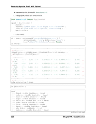
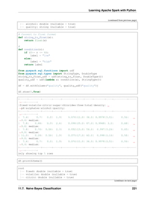
![Learning Apache Spark with Python
(continued from previous page)
|-- sugar: double (nullable = true)
|-- chlorides: double (nullable = true)
|-- free: double (nullable = true)
|-- total: double (nullable = true)
|-- density: double (nullable = true)
|-- pH: double (nullable = true)
|-- sulphates: double (nullable = true)
|-- alcohol: double (nullable = true)
|-- quality: string (nullable = true)
3. Deal with categorical data and Convert the data to dense vector
Note:
You are strongly encouraged to try my get_dummy function for dealing with the categorical
data in complex dataset.
Supervised learning version:
def get_dummy(df,indexCol,categoricalCols,continuousCols,
˓
→labelCol):
from pyspark.ml import Pipeline
from pyspark.ml.feature import StringIndexer,
˓
→OneHotEncoder, VectorAssembler
from pyspark.sql.functions import col
indexers = [ StringIndexer(inputCol=c, outputCol="{0}_
˓
→indexed".format(c))
for c in categoricalCols ]
# default setting: dropLast=True
encoders = [ OneHotEncoder(inputCol=indexer.
˓
→getOutputCol(),
outputCol="{0}_encoded".format(indexer.
˓
→getOutputCol()))
for indexer in indexers ]
assembler = VectorAssembler(inputCols=[encoder.
˓
→getOutputCol() for encoder in encoders]
+ continuousCols, outputCol=
˓
→"features")
pipeline = Pipeline(stages=indexers + encoders +
˓
→[assembler])
model=pipeline.fit(df)
data = model.transform(df)
data = data.withColumn('label',col(labelCol))
return data.select(indexCol,'features','label')
222 Chapter 11. Classification](https://image.slidesharecdn.com/pyspark-230429134708-b35c8a19/85/pyspark-pdf-228-320.jpg)
![Learning Apache Spark with Python
Unsupervised learning version:
def get_dummy(df,indexCol,categoricalCols,continuousCols):
'''
Get dummy variables and concat with continuous variables
˓
→for unsupervised learning.
:param df: the dataframe
:param categoricalCols: the name list of the categorical
˓
→data
:param continuousCols: the name list of the numerical
˓
→data
:return k: feature matrix
:author: Wenqiang Feng
:email: von198@gmail.com
'''
indexers = [ StringIndexer(inputCol=c, outputCol="{0}_
˓
→indexed".format(c))
for c in categoricalCols ]
# default setting: dropLast=True
encoders = [ OneHotEncoder(inputCol=indexer.
˓
→getOutputCol(),
outputCol="{0}_encoded".format(indexer.
˓
→getOutputCol()))
for indexer in indexers ]
assembler = VectorAssembler(inputCols=[encoder.
˓
→getOutputCol() for encoder in encoders]
+ continuousCols, outputCol=
˓
→"features")
pipeline = Pipeline(stages=indexers + encoders +
˓
→[assembler])
model=pipeline.fit(df)
data = model.transform(df)
return data.select(indexCol,'features')
Two in one:
def get_dummy(df,indexCol,categoricalCols,continuousCols,labelCol,
˓
→dropLast=False):
'''
Get dummy variables and concat with continuous variables for ml
˓
→modeling.
:param df: the dataframe
:param categoricalCols: the name list of the categorical data
:param continuousCols: the name list of the numerical data
:param labelCol: the name of label column
(continues on next page)
11.7. Naive Bayes Classification 223](https://image.slidesharecdn.com/pyspark-230429134708-b35c8a19/85/pyspark-pdf-229-320.jpg)
![Learning Apache Spark with Python
(continued from previous page)
:param dropLast: the flag of drop last column
:return: feature matrix
:author: Wenqiang Feng
:email: von198@gmail.com
>>> df = spark.createDataFrame([
(0, "a"),
(1, "b"),
(2, "c"),
(3, "a"),
(4, "a"),
(5, "c")
], ["id", "category"])
>>> indexCol = 'id'
>>> categoricalCols = ['category']
>>> continuousCols = []
>>> labelCol = []
>>> mat = get_dummy(df,indexCol,categoricalCols,continuousCols,
˓
→labelCol)
>>> mat.show()
>>>
+---+-------------+
| id| features|
+---+-------------+
| 0|[1.0,0.0,0.0]|
| 1|[0.0,0.0,1.0]|
| 2|[0.0,1.0,0.0]|
| 3|[1.0,0.0,0.0]|
| 4|[1.0,0.0,0.0]|
| 5|[0.0,1.0,0.0]|
+---+-------------+
'''
from pyspark.ml import Pipeline
from pyspark.ml.feature import StringIndexer, OneHotEncoder,
˓
→VectorAssembler
from pyspark.sql.functions import col
indexers = [ StringIndexer(inputCol=c, outputCol="{0}_indexed".
˓
→format(c))
for c in categoricalCols ]
# default setting: dropLast=True
encoders = [ OneHotEncoder(inputCol=indexer.getOutputCol(),
outputCol="{0}_encoded".format(indexer.
˓
→getOutputCol()),dropLast=dropLast)
for indexer in indexers ]
(continues on next page)
224 Chapter 11. Classification](https://image.slidesharecdn.com/pyspark-230429134708-b35c8a19/85/pyspark-pdf-230-320.jpg)
![Learning Apache Spark with Python
(continued from previous page)
assembler = VectorAssembler(inputCols=[encoder.getOutputCol()
˓
→for encoder in encoders]
+ continuousCols, outputCol="features
˓
→")
pipeline = Pipeline(stages=indexers + encoders + [assembler])
model=pipeline.fit(df)
data = model.transform(df)
if indexCol and labelCol:
# for supervised learning
data = data.withColumn('label',col(labelCol))
return data.select(indexCol,'features','label')
elif not indexCol and labelCol:
# for supervised learning
data = data.withColumn('label',col(labelCol))
return data.select('features','label')
elif indexCol and not labelCol:
# for unsupervised learning
return data.select(indexCol,'features')
elif not indexCol and not labelCol:
# for unsupervised learning
return data.select('features')
def get_dummy(df,categoricalCols,continuousCols,labelCol):
from pyspark.ml import Pipeline
from pyspark.ml.feature import StringIndexer, OneHotEncoder,
˓
→VectorAssembler
from pyspark.sql.functions import col
indexers = [ StringIndexer(inputCol=c, outputCol="{0}_indexed".format(c))
for c in categoricalCols ]
# default setting: dropLast=True
encoders = [ OneHotEncoder(inputCol=indexer.getOutputCol(),
outputCol="{0}_encoded".format(indexer.getOutputCol()))
for indexer in indexers ]
assembler = VectorAssembler(inputCols=[encoder.getOutputCol() for encoder
˓
→in encoders]
+ continuousCols, outputCol="features")
pipeline = Pipeline(stages=indexers + encoders + [assembler])
model=pipeline.fit(df)
data = model.transform(df)
data = data.withColumn('label',col(labelCol))
(continues on next page)
11.7. Naive Bayes Classification 225](https://image.slidesharecdn.com/pyspark-230429134708-b35c8a19/85/pyspark-pdf-231-320.jpg)
![Learning Apache Spark with Python
(continued from previous page)
return data.select('features','label')
4. Transform the dataset to DataFrame
from pyspark.ml.linalg import Vectors # !!!!caution: not from pyspark.mllib.
˓
→linalg import Vectors
from pyspark.ml import Pipeline
from pyspark.ml.feature import IndexToString,StringIndexer, VectorIndexer
from pyspark.ml.tuning import CrossValidator, ParamGridBuilder
from pyspark.ml.evaluation import MulticlassClassificationEvaluator
def transData(data):
return data.rdd.map(lambda r: [Vectors.dense(r[:-1]),r[-1]]).toDF(['features',
˓
→'label'])
transformed = transData(df)
transformed.show(5)
+--------------------+-----+
| features|label|
+--------------------+-----+
|[7.4,0.7,0.0,1.9,...| low|
|[7.8,0.88,0.0,2.6...| low|
|[7.8,0.76,0.04,2....| low|
|[11.2,0.28,0.56,1...| low|
|[7.4,0.7,0.0,1.9,...| low|
+--------------------+-----+
only showing top 5 rows
4. Deal with Categorical Label and Variables
# Index labels, adding metadata to the label column
labelIndexer = StringIndexer(inputCol='label',
outputCol='indexedLabel').fit(transformed)
labelIndexer.transform(transformed).show(5, True)
+--------------------+-----+------------+
| features|label|indexedLabel|
+--------------------+-----+------------+
|[7.4,0.7,0.0,1.9,...| low| 0.0|
|[7.8,0.88,0.0,2.6...| low| 0.0|
|[7.8,0.76,0.04,2....| low| 0.0|
|[11.2,0.28,0.56,1...| low| 0.0|
|[7.4,0.7,0.0,1.9,...| low| 0.0|
+--------------------+-----+------------+
only showing top 5 rows
# Automatically identify categorical features, and index them.
# Set maxCategories so features with > 4 distinct values are treated as
˓
→continuous. (continues on next page)
226 Chapter 11. Classification](https://image.slidesharecdn.com/pyspark-230429134708-b35c8a19/85/pyspark-pdf-232-320.jpg)
![Learning Apache Spark with Python
(continued from previous page)
featureIndexer =VectorIndexer(inputCol="features",
outputCol="indexedFeatures",
maxCategories=4).fit(transformed)
featureIndexer.transform(transformed).show(5, True)
+--------------------+-----+--------------------+
| features|label| indexedFeatures|
+--------------------+-----+--------------------+
|[7.4,0.7,0.0,1.9,...| low|[7.4,0.7,0.0,1.9,...|
|[7.8,0.88,0.0,2.6...| low|[7.8,0.88,0.0,2.6...|
|[7.8,0.76,0.04,2....| low|[7.8,0.76,0.04,2....|
|[11.2,0.28,0.56,1...| low|[11.2,0.28,0.56,1...|
|[7.4,0.7,0.0,1.9,...| low|[7.4,0.7,0.0,1.9,...|
+--------------------+-----+--------------------+
only showing top 5 rows
5. Split the data to training and test data sets
# Split the data into training and test sets (40% held out for testing)
(trainingData, testData) = data.randomSplit([0.6, 0.4])
trainingData.show(5,False)
testData.show(5,False)
+---------------------------------------------------------+-----+
|features |label|
+---------------------------------------------------------+-----+
|[5.0,0.38,0.01,1.6,0.048,26.0,60.0,0.99084,3.7,0.75,14.0]|low |
|[5.0,0.42,0.24,2.0,0.06,19.0,50.0,0.9917,3.72,0.74,14.0] |high |
|[5.0,0.74,0.0,1.2,0.041,16.0,46.0,0.99258,4.01,0.59,12.5]|low |
|[5.0,1.02,0.04,1.4,0.045,41.0,85.0,0.9938,3.75,0.48,10.5]|low |
|[5.0,1.04,0.24,1.6,0.05,32.0,96.0,0.9934,3.74,0.62,11.5] |low |
+---------------------------------------------------------+-----+
only showing top 5 rows
+---------------------------------------------------------+-----+
|features |label|
+---------------------------------------------------------+-----+
|[4.6,0.52,0.15,2.1,0.054,8.0,65.0,0.9934,3.9,0.56,13.1] |low |
|[4.7,0.6,0.17,2.3,0.058,17.0,106.0,0.9932,3.85,0.6,12.9] |low |
|[4.9,0.42,0.0,2.1,0.048,16.0,42.0,0.99154,3.71,0.74,14.0]|high |
|[5.0,0.4,0.5,4.3,0.046,29.0,80.0,0.9902,3.49,0.66,13.6] |low |
|[5.2,0.49,0.26,2.3,0.09,23.0,74.0,0.9953,3.71,0.62,12.2] |low |
+---------------------------------------------------------+-----+
only showing top 5 rows
6. Fit Naive Bayes Classification Model
from pyspark.ml.classification import NaiveBayes
nb = NaiveBayes(featuresCol='indexedFeatures', labelCol='indexedLabel')
11.7. Naive Bayes Classification 227](https://image.slidesharecdn.com/pyspark-230429134708-b35c8a19/85/pyspark-pdf-233-320.jpg)
![Learning Apache Spark with Python
7. Pipeline Architecture
# Convert indexed labels back to original labels.
labelConverter = IndexToString(inputCol="prediction", outputCol=
˓
→"predictedLabel",
labels=labelIndexer.labels)
# Chain indexers and tree in a Pipeline
pipeline = Pipeline(stages=[labelIndexer, featureIndexer, nb,labelConverter])
# Train model. This also runs the indexers.
model = pipeline.fit(trainingData)
8. Make predictions
# Make predictions.
predictions = model.transform(testData)
# Select example rows to display.
predictions.select("features","label","predictedLabel").show(5)
+--------------------+-----+--------------+
| features|label|predictedLabel|
+--------------------+-----+--------------+
|[4.6,0.52,0.15,2....| low| low|
|[4.7,0.6,0.17,2.3...| low| low|
|[4.9,0.42,0.0,2.1...| high| low|
|[5.0,0.4,0.5,4.3,...| low| low|
|[5.2,0.49,0.26,2....| low| low|
+--------------------+-----+--------------+
only showing top 5 rows
9. Evaluation
from pyspark.ml.evaluation import MulticlassClassificationEvaluator
# Select (prediction, true label) and compute test error
evaluator = MulticlassClassificationEvaluator(
labelCol="indexedLabel", predictionCol="prediction", metricName="accuracy
˓
→")
accuracy = evaluator.evaluate(predictions)
print("Test Error = %g" % (1.0 - accuracy))
Test Error = 0.307339
lrModel = model.stages[2]
trainingSummary = lrModel.summary
# Obtain the objective per iteration
# objectiveHistory = trainingSummary.objectiveHistory
# print("objectiveHistory:")
# for objective in objectiveHistory:
(continues on next page)
228 Chapter 11. Classification](https://image.slidesharecdn.com/pyspark-230429134708-b35c8a19/85/pyspark-pdf-234-320.jpg)
![Learning Apache Spark with Python
(continued from previous page)
# print(objective)
# Obtain the receiver-operating characteristic as a dataframe and
˓
→areaUnderROC.
trainingSummary.roc.show(5)
print("areaUnderROC: " + str(trainingSummary.areaUnderROC))
# Set the model threshold to maximize F-Measure
fMeasure = trainingSummary.fMeasureByThreshold
maxFMeasure = fMeasure.groupBy().max('F-Measure').select('max(F-Measure)').
˓
→head(5)
# bestThreshold = fMeasure.where(fMeasure['F-Measure'] == maxFMeasure['max(F-
˓
→Measure)'])
# .select('threshold').head()['threshold']
# lr.setThreshold(bestThreshold)
You can use z.show() to get the data and plot the ROC curves:
You can also register a TempTable data.registerTempTable('roc_data') and then use sql to
plot the ROC curve:
11.7. Naive Bayes Classification 229](https://image.slidesharecdn.com/pyspark-230429134708-b35c8a19/85/pyspark-pdf-235-320.jpg)
![Learning Apache Spark with Python
10. visualization
import matplotlib.pyplot as plt
import numpy as np
import itertools
def plot_confusion_matrix(cm, classes,
normalize=False,
title='Confusion matrix',
cmap=plt.cm.Blues):
"""
This function prints and plots the confusion matrix.
Normalization can be applied by setting `normalize=True`.
"""
if normalize:
cm = cm.astype('float') / cm.sum(axis=1)[:, np.newaxis]
print("Normalized confusion matrix")
else:
print('Confusion matrix, without normalization')
print(cm)
plt.imshow(cm, interpolation='nearest', cmap=cmap)
plt.title(title)
plt.colorbar()
tick_marks = np.arange(len(classes))
plt.xticks(tick_marks, classes, rotation=45)
plt.yticks(tick_marks, classes)
fmt = '.2f' if normalize else 'd'
thresh = cm.max() / 2.
for i, j in itertools.product(range(cm.shape[0]), range(cm.shape[1])):
plt.text(j, i, format(cm[i, j], fmt),
horizontalalignment="center",
color="white" if cm[i, j] > thresh else "black")
plt.tight_layout()
plt.ylabel('True label')
plt.xlabel('Predicted label')
class_temp = predictions.select("label").groupBy("label")
.count().sort('count', ascending=False).toPandas()
class_temp = class_temp["label"].values.tolist()
class_names = map(str, class_temp)
# # # print(class_name)
class_names
['low', 'high']
from sklearn.metrics import confusion_matrix
y_true = predictions.select("label")
y_true = y_true.toPandas()
(continues on next page)
230 Chapter 11. Classification](https://image.slidesharecdn.com/pyspark-230429134708-b35c8a19/85/pyspark-pdf-236-320.jpg)
![Learning Apache Spark with Python
(continued from previous page)
y_pred = predictions.select("predictedLabel")
y_pred = y_pred.toPandas()
cnf_matrix = confusion_matrix(y_true, y_pred,labels=class_names)
cnf_matrix
array([[392, 169],
[ 32, 61]])
# Plot non-normalized confusion matrix
plt.figure()
plot_confusion_matrix(cnf_matrix, classes=class_names,
title='Confusion matrix, without normalization')
plt.show()
Confusion matrix, without normalization
[[392 169]
[ 32 61]]
# Plot normalized confusion matrix
plt.figure()
plot_confusion_matrix(cnf_matrix, classes=class_names, normalize=True,
title='Normalized confusion matrix')
(continues on next page)
11.7. Naive Bayes Classification 231](https://image.slidesharecdn.com/pyspark-230429134708-b35c8a19/85/pyspark-pdf-237-320.jpg)
![Learning Apache Spark with Python
(continued from previous page)
plt.show()
Normalized confusion matrix
[[0.69875223 0.30124777]
[0.34408602 0.65591398]]
232 Chapter 11. Classification](https://image.slidesharecdn.com/pyspark-230429134708-b35c8a19/85/pyspark-pdf-238-320.jpg)
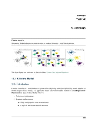
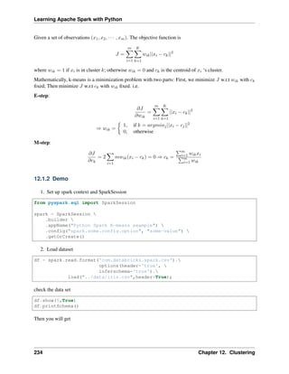
![Learning Apache Spark with Python
+------------+-----------+------------+-----------+-------+
|sepal_length|sepal_width|petal_length|petal_width|species|
+------------+-----------+------------+-----------+-------+
| 5.1| 3.5| 1.4| 0.2| setosa|
| 4.9| 3.0| 1.4| 0.2| setosa|
| 4.7| 3.2| 1.3| 0.2| setosa|
| 4.6| 3.1| 1.5| 0.2| setosa|
| 5.0| 3.6| 1.4| 0.2| setosa|
+------------+-----------+------------+-----------+-------+
only showing top 5 rows
root
|-- sepal_length: double (nullable = true)
|-- sepal_width: double (nullable = true)
|-- petal_length: double (nullable = true)
|-- petal_width: double (nullable = true)
|-- species: string (nullable = true)
You can also get the Statistical resutls from the data frame (Unfortunately, it only works for numerical).
df.describe().show()
Then you will get
+-------+------------------+-------------------+------------------+-----------
˓
→-------+---------+
|summary| sepal_length| sepal_width| petal_length|
˓
→petal_width| species|
+-------+------------------+-------------------+------------------+-----------
˓
→-------+---------+
| count| 150| 150| 150|
˓
→ 150| 150|
| mean| 5.843333333333335| 3.0540000000000007|3.7586666666666693|1.
˓
→1986666666666672| null|
| stddev|0.8280661279778637|0.43359431136217375| 1.764420419952262|0.
˓
→7631607417008414| null|
| min| 4.3| 2.0| 1.0|
˓
→ 0.1| setosa|
| max| 7.9| 4.4| 6.9|
˓
→ 2.5|virginica|
+-------+------------------+-------------------+------------------+-----------
˓
→-------+---------+
3. Convert the data to dense vector (features)
# convert the data to dense vector
from pyspark.mllib.linalg import Vectors
def transData(data):
return data.rdd.map(lambda r: [Vectors.dense(r[:-1])]).toDF(['features'])
Note:
12.1. K-Means Model 235](https://image.slidesharecdn.com/pyspark-230429134708-b35c8a19/85/pyspark-pdf-241-320.jpg)
![Learning Apache Spark with Python
You are strongly encouraged to try my get_dummy function for dealing with the categorical
data in complex dataset.
Supervised learning version:
def get_dummy(df,indexCol,categoricalCols,continuousCols,
˓
→labelCol):
from pyspark.ml import Pipeline
from pyspark.ml.feature import StringIndexer,
˓
→OneHotEncoder, VectorAssembler
from pyspark.sql.functions import col
indexers = [ StringIndexer(inputCol=c, outputCol="{0}_
˓
→indexed".format(c))
for c in categoricalCols ]
# default setting: dropLast=True
encoders = [ OneHotEncoder(inputCol=indexer.
˓
→getOutputCol(),
outputCol="{0}_encoded".format(indexer.
˓
→getOutputCol()))
for indexer in indexers ]
assembler = VectorAssembler(inputCols=[encoder.
˓
→getOutputCol() for encoder in encoders]
+ continuousCols, outputCol=
˓
→"features")
pipeline = Pipeline(stages=indexers + encoders +
˓
→[assembler])
model=pipeline.fit(df)
data = model.transform(df)
data = data.withColumn('label',col(labelCol))
return data.select(indexCol,'features','label')
Unsupervised learning version:
def get_dummy(df,indexCol,categoricalCols,continuousCols):
'''
Get dummy variables and concat with continuous variables
˓
→for unsupervised learning.
:param df: the dataframe
:param categoricalCols: the name list of the categorical
˓
→data
:param continuousCols: the name list of the numerical
˓
→data
:return k: feature matrix
:author: Wenqiang Feng
(continues on next page)
236 Chapter 12. Clustering](https://image.slidesharecdn.com/pyspark-230429134708-b35c8a19/85/pyspark-pdf-242-320.jpg)
![Learning Apache Spark with Python
(continued from previous page)
:email: von198@gmail.com
'''
indexers = [ StringIndexer(inputCol=c, outputCol="{0}_
˓
→indexed".format(c))
for c in categoricalCols ]
# default setting: dropLast=True
encoders = [ OneHotEncoder(inputCol=indexer.
˓
→getOutputCol(),
outputCol="{0}_encoded".format(indexer.
˓
→getOutputCol()))
for indexer in indexers ]
assembler = VectorAssembler(inputCols=[encoder.
˓
→getOutputCol() for encoder in encoders]
+ continuousCols, outputCol=
˓
→"features")
pipeline = Pipeline(stages=indexers + encoders +
˓
→[assembler])
model=pipeline.fit(df)
data = model.transform(df)
return data.select(indexCol,'features')
Two in one:
def get_dummy(df,indexCol,categoricalCols,continuousCols,labelCol,
˓
→dropLast=False):
'''
Get dummy variables and concat with continuous variables for ml
˓
→modeling.
:param df: the dataframe
:param categoricalCols: the name list of the categorical data
:param continuousCols: the name list of the numerical data
:param labelCol: the name of label column
:param dropLast: the flag of drop last column
:return: feature matrix
:author: Wenqiang Feng
:email: von198@gmail.com
>>> df = spark.createDataFrame([
(0, "a"),
(1, "b"),
(2, "c"),
(3, "a"),
(4, "a"),
(5, "c")
(continues on next page)
12.1. K-Means Model 237](https://image.slidesharecdn.com/pyspark-230429134708-b35c8a19/85/pyspark-pdf-243-320.jpg)
![Learning Apache Spark with Python
(continued from previous page)
], ["id", "category"])
>>> indexCol = 'id'
>>> categoricalCols = ['category']
>>> continuousCols = []
>>> labelCol = []
>>> mat = get_dummy(df,indexCol,categoricalCols,continuousCols,
˓
→labelCol)
>>> mat.show()
>>>
+---+-------------+
| id| features|
+---+-------------+
| 0|[1.0,0.0,0.0]|
| 1|[0.0,0.0,1.0]|
| 2|[0.0,1.0,0.0]|
| 3|[1.0,0.0,0.0]|
| 4|[1.0,0.0,0.0]|
| 5|[0.0,1.0,0.0]|
+---+-------------+
'''
from pyspark.ml import Pipeline
from pyspark.ml.feature import StringIndexer, OneHotEncoder,
˓
→VectorAssembler
from pyspark.sql.functions import col
indexers = [ StringIndexer(inputCol=c, outputCol="{0}_indexed".
˓
→format(c))
for c in categoricalCols ]
# default setting: dropLast=True
encoders = [ OneHotEncoder(inputCol=indexer.getOutputCol(),
outputCol="{0}_encoded".format(indexer.
˓
→getOutputCol()),dropLast=dropLast)
for indexer in indexers ]
assembler = VectorAssembler(inputCols=[encoder.getOutputCol()
˓
→for encoder in encoders]
+ continuousCols, outputCol="features
˓
→")
pipeline = Pipeline(stages=indexers + encoders + [assembler])
model=pipeline.fit(df)
data = model.transform(df)
if indexCol and labelCol:
# for supervised learning
data = data.withColumn('label',col(labelCol))
(continues on next page)
238 Chapter 12. Clustering](https://image.slidesharecdn.com/pyspark-230429134708-b35c8a19/85/pyspark-pdf-244-320.jpg)
![Learning Apache Spark with Python
(continued from previous page)
return data.select(indexCol,'features','label')
elif not indexCol and labelCol:
# for supervised learning
data = data.withColumn('label',col(labelCol))
return data.select('features','label')
elif indexCol and not labelCol:
# for unsupervised learning
return data.select(indexCol,'features')
elif not indexCol and not labelCol:
# for unsupervised learning
return data.select('features')
4. Transform the dataset to DataFrame
transformed= transData(df)
transformed.show(5, False)
+-----------------+
|features |
+-----------------+
|[5.1,3.5,1.4,0.2]|
|[4.9,3.0,1.4,0.2]|
|[4.7,3.2,1.3,0.2]|
|[4.6,3.1,1.5,0.2]|
|[5.0,3.6,1.4,0.2]|
+-----------------+
only showing top 5 rows
5. Deal With Categorical Variables
from pyspark.ml import Pipeline
from pyspark.ml.regression import LinearRegression
from pyspark.ml.feature import VectorIndexer
from pyspark.ml.evaluation import RegressionEvaluator
# Automatically identify categorical features, and index them.
# We specify maxCategories so features with > 4 distinct values are treated
˓
→as continuous.
featureIndexer = VectorIndexer(inputCol="features",
outputCol="indexedFeatures",
maxCategories=4).fit(transformed)
data = featureIndexer.transform(transformed)
Now you check your dataset with
data.show(5,True)
you will get
12.1. K-Means Model 239](https://image.slidesharecdn.com/pyspark-230429134708-b35c8a19/85/pyspark-pdf-245-320.jpg)
![Learning Apache Spark with Python
+-----------------+-----------------+
| features| indexedFeatures|
+-----------------+-----------------+
|[5.1,3.5,1.4,0.2]|[5.1,3.5,1.4,0.2]|
|[4.9,3.0,1.4,0.2]|[4.9,3.0,1.4,0.2]|
|[4.7,3.2,1.3,0.2]|[4.7,3.2,1.3,0.2]|
|[4.6,3.1,1.5,0.2]|[4.6,3.1,1.5,0.2]|
|[5.0,3.6,1.4,0.2]|[5.0,3.6,1.4,0.2]|
+-----------------+-----------------+
only showing top 5 rows
Note: Since clustering algorithms including k-means use distance-based measurements to determine the
similarity between data points, It’s strongly recommended to standardize the data to have a mean of zero
and a standard deviation of one.
6. Elbow method to determine the optimal number of clusters for k-means clustering
import numpy as np
cost = np.zeros(20)
for k in range(2,20):
kmeans = KMeans()
.setK(k)
.setSeed(1)
.setFeaturesCol("indexedFeatures")
.setPredictionCol("cluster")
model = kmeans.fit(data)
cost[k] = model.computeCost(data) # requires Spark 2.0 or later
import numpy as np
import matplotlib.mlab as mlab
import matplotlib.pyplot as plt
import seaborn as sbs
from matplotlib.ticker import MaxNLocator
fig, ax = plt.subplots(1,1, figsize =(8,6))
ax.plot(range(2,20),cost[2:20])
ax.set_xlabel('k')
ax.set_ylabel('cost')
ax.xaxis.set_major_locator(MaxNLocator(integer=True))
plt.show()
240 Chapter 12. Clustering](https://image.slidesharecdn.com/pyspark-230429134708-b35c8a19/85/pyspark-pdf-246-320.jpg)
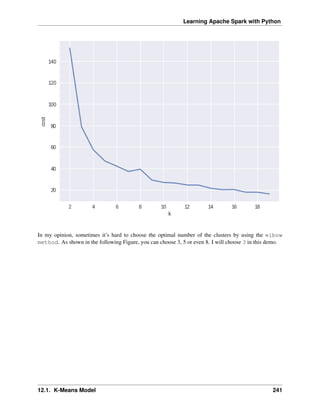
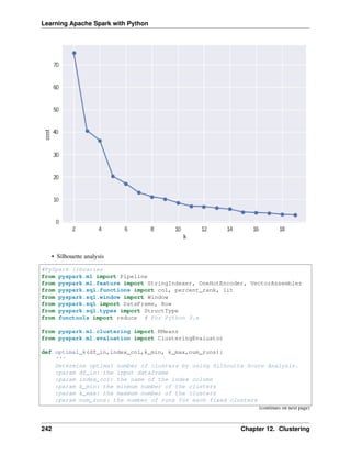
![Learning Apache Spark with Python
(continued from previous page)
:return k: optimal number of the clusters
:return silh_lst: Silhouette score
:return r_table: the running results table
:author: Wenqiang Feng
:email: von198@gmail.com
'''
start = time.time()
silh_lst = []
k_lst = np.arange(k_min, k_max+1)
r_table = df_in.select(index_col).toPandas()
r_table = r_table.set_index(index_col)
centers = pd.DataFrame()
for k in k_lst:
silh_val = []
for run in np.arange(1, num_runs+1):
# Trains a k-means model.
kmeans = KMeans()
.setK(k)
.setSeed(int(np.random.randint(100, size=1)))
model = kmeans.fit(df_in)
# Make predictions
predictions = model.transform(df_in)
r_table['cluster_{k}_{run}'.format(k=k, run=run)]= predictions.
˓
→select('prediction').toPandas()
# Evaluate clustering by computing Silhouette score
evaluator = ClusteringEvaluator()
silhouette = evaluator.evaluate(predictions)
silh_val.append(silhouette)
silh_array=np.asanyarray(silh_val)
silh_lst.append(silh_array.mean())
elapsed = time.time() - start
silhouette = pd.DataFrame(list(zip(k_lst,silh_lst)),columns = ['k',
˓
→'silhouette'])
print('+------------------------------------------------------------+')
print("| The finding optimal k phase took %8.0f s. |"
˓
→%(elapsed))
print('+------------------------------------------------------------+')
return k_lst[np.argmax(silh_lst, axis=0)], silhouette , r_table
12.1. K-Means Model 243](https://image.slidesharecdn.com/pyspark-230429134708-b35c8a19/85/pyspark-pdf-249-320.jpg)
![Learning Apache Spark with Python
k, silh_lst, r_table = optimal_k(scaledData,index_col,k_min, k_max,num_runs)
+------------------------------------------------------------+
| The finding optimal k phase took 1783 s. |
+------------------------------------------------------------+
spark.createDataFrame(silh_lst).show()
+---+------------------+
| k| silhouette|
+---+------------------+
| 3|0.8045154385557953|
| 4|0.6993528775512052|
| 5|0.6689286654221447|
| 6|0.6356184024841809|
| 7|0.7174102265711756|
| 8|0.6720861758298997|
| 9| 0.601771359881241|
| 10|0.6292447334578428|
+---+------------------+
From the silhouette list, we can choose 3 as the optimal number of the clusters.
Warning: ClusteringEvaluator in pyspark.ml.evaluation requires Spark 2.4 or later!!
7. Pipeline Architecture
from pyspark.ml.clustering import KMeans, KMeansModel
kmeans = KMeans()
.setK(3)
.setFeaturesCol("indexedFeatures")
.setPredictionCol("cluster")
# Chain indexer and tree in a Pipeline
pipeline = Pipeline(stages=[featureIndexer, kmeans])
model = pipeline.fit(transformed)
cluster = model.transform(transformed)
8. k-means clusters
cluster = model.transform(transformed)
+-----------------+-----------------+-------+
| features| indexedFeatures|cluster|
+-----------------+-----------------+-------+
|[5.1,3.5,1.4,0.2]|[5.1,3.5,1.4,0.2]| 1|
|[4.9,3.0,1.4,0.2]|[4.9,3.0,1.4,0.2]| 1|
(continues on next page)
244 Chapter 12. Clustering](https://image.slidesharecdn.com/pyspark-230429134708-b35c8a19/85/pyspark-pdf-250-320.jpg)
![Learning Apache Spark with Python
(continued from previous page)
|[4.7,3.2,1.3,0.2]|[4.7,3.2,1.3,0.2]| 1|
|[4.6,3.1,1.5,0.2]|[4.6,3.1,1.5,0.2]| 1|
|[5.0,3.6,1.4,0.2]|[5.0,3.6,1.4,0.2]| 1|
|[5.4,3.9,1.7,0.4]|[5.4,3.9,1.7,0.4]| 1|
|[4.6,3.4,1.4,0.3]|[4.6,3.4,1.4,0.3]| 1|
|[5.0,3.4,1.5,0.2]|[5.0,3.4,1.5,0.2]| 1|
|[4.4,2.9,1.4,0.2]|[4.4,2.9,1.4,0.2]| 1|
|[4.9,3.1,1.5,0.1]|[4.9,3.1,1.5,0.1]| 1|
|[5.4,3.7,1.5,0.2]|[5.4,3.7,1.5,0.2]| 1|
|[4.8,3.4,1.6,0.2]|[4.8,3.4,1.6,0.2]| 1|
|[4.8,3.0,1.4,0.1]|[4.8,3.0,1.4,0.1]| 1|
|[4.3,3.0,1.1,0.1]|[4.3,3.0,1.1,0.1]| 1|
|[5.8,4.0,1.2,0.2]|[5.8,4.0,1.2,0.2]| 1|
|[5.7,4.4,1.5,0.4]|[5.7,4.4,1.5,0.4]| 1|
|[5.4,3.9,1.3,0.4]|[5.4,3.9,1.3,0.4]| 1|
|[5.1,3.5,1.4,0.3]|[5.1,3.5,1.4,0.3]| 1|
|[5.7,3.8,1.7,0.3]|[5.7,3.8,1.7,0.3]| 1|
|[5.1,3.8,1.5,0.3]|[5.1,3.8,1.5,0.3]| 1|
+-----------------+-----------------+-------+
only showing top 20 rows
12.1. K-Means Model 245](https://image.slidesharecdn.com/pyspark-230429134708-b35c8a19/85/pyspark-pdf-251-320.jpg)

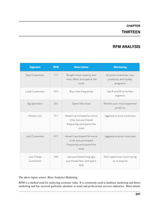
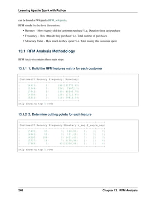
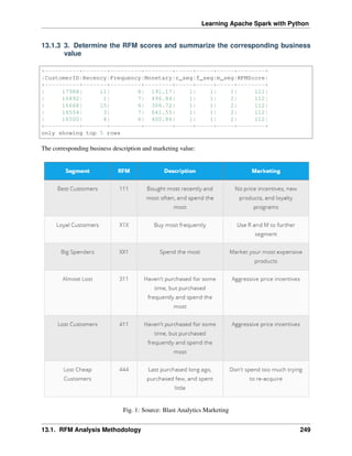
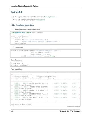
![Learning Apache Spark with Python
(continued from previous page)
root
|-- InvoiceNo: string (nullable = true)
|-- StockCode: string (nullable = true)
|-- Description: string (nullable = true)
|-- Quantity: integer (nullable = true)
|-- InvoiceDate: string (nullable = true)
|-- UnitPrice: double (nullable = true)
|-- CustomerID: integer (nullable = true)
|-- Country: string (nullable = true)
3. Data clean and data manipulation
• check and remove the null values
from pyspark.sql.functions import count
def my_count(df_in):
df_in.agg( *[ count(c).alias(c) for c in df_in.columns ] ).show()
my_count(df_raw)
+---------+---------+-----------+--------+-----------+---------+----------+---
˓
→----+
|InvoiceNo|StockCode|Description|Quantity|InvoiceDate|UnitPrice|CustomerID|Country|
+---------+---------+-----------+--------+-----------+---------+----------+---
˓
→----+
| 541909| 541909| 540455| 541909| 541909| 541909| 406829|
˓
→541909|
+---------+---------+-----------+--------+-----------+---------+----------+---
˓
→----+
Since the count results are not the same, we have some null value in the CustomerID column. We can
drop these records from the dataset.
df = df_raw.dropna(how='any')
my_count(df)
+---------+---------+-----------+--------+-----------+---------+----------+---
˓
→----+
|InvoiceNo|StockCode|Description|Quantity|InvoiceDate|UnitPrice|CustomerID|Country|
+---------+---------+-----------+--------+-----------+---------+----------+---
˓
→----+
| 406829| 406829| 406829| 406829| 406829| 406829| 406829|
˓
→406829|
+---------+---------+-----------+--------+-----------+---------+----------+---
˓
→----+
• Dealwith the InvoiceDate
13.2. Demo 251](https://image.slidesharecdn.com/pyspark-230429134708-b35c8a19/85/pyspark-pdf-257-320.jpg)
![Learning Apache Spark with Python
from pyspark.sql.functions import to_utc_timestamp, unix_timestamp, lit,
˓
→datediff, col
timeFmt = "MM/dd/yy HH:mm"
df = df.withColumn('NewInvoiceDate'
, to_utc_timestamp(unix_timestamp(col('InvoiceDate'),
˓
→timeFmt).cast('timestamp')
, 'UTC'))
df.show(5)
+---------+---------+--------------------+--------+------------+---------+----
˓
→------+--------------+--------------------+
|InvoiceNo|StockCode| Description|Quantity|
˓
→InvoiceDate|UnitPrice|CustomerID| Country| NewInvoiceDate|
+---------+---------+--------------------+--------+------------+---------+----
˓
→------+--------------+--------------------+
| 536365| 85123A|WHITE HANGING HEA...| 6|12/1/10 8:26| 2.55|
˓
→ 17850|United Kingdom|2010-12-01 08:26:...|
| 536365| 71053| WHITE METAL LANTERN| 6|12/1/10 8:26| 3.39|
˓
→ 17850|United Kingdom|2010-12-01 08:26:...|
| 536365| 84406B|CREAM CUPID HEART...| 8|12/1/10 8:26| 2.75|
˓
→ 17850|United Kingdom|2010-12-01 08:26:...|
| 536365| 84029G|KNITTED UNION FLA...| 6|12/1/10 8:26| 3.39|
˓
→ 17850|United Kingdom|2010-12-01 08:26:...|
| 536365| 84029E|RED WOOLLY HOTTIE...| 6|12/1/10 8:26| 3.39|
˓
→ 17850|United Kingdom|2010-12-01 08:26:...|
+---------+---------+--------------------+--------+------------+---------+----
˓
→------+--------------+--------------------+
only showing top 5 rows
Warning: The spark is pretty sensitive to the date format!
• calculate total price
from pyspark.sql.functions import round
df = df.withColumn('TotalPrice', round( df.Quantity * df.UnitPrice, 2 ) )
• calculate the time difference
from pyspark.sql.functions import mean, min, max, sum, datediff, to_date
date_max = df.select(max('NewInvoiceDate')).toPandas()
current = to_utc_timestamp( unix_timestamp(lit(str(date_max.iloc[0][0])),
'yy-MM-dd HH:mm').cast('timestamp'), 'UTC' )
# Calculatre Duration
df = df.withColumn('Duration', datediff(lit(current), 'NewInvoiceDate'))
252 Chapter 13. RFM Analysis](https://image.slidesharecdn.com/pyspark-230429134708-b35c8a19/85/pyspark-pdf-258-320.jpg)
![Learning Apache Spark with Python
• build the Recency, Frequency and Monetary
recency = df.groupBy('CustomerID').agg(min('Duration').alias('Recency'))
frequency = df.groupBy('CustomerID', 'InvoiceNo').count()
.groupBy('CustomerID')
.agg(count("*").alias("Frequency"))
monetary = df.groupBy('CustomerID').agg(round(sum('TotalPrice'), 2).alias(
˓
→'Monetary'))
rfm = recency.join(frequency,'CustomerID', how = 'inner')
.join(monetary,'CustomerID', how = 'inner')
rfm.show(5)
+----------+-------+---------+--------+
|CustomerID|Recency|Frequency|Monetary|
+----------+-------+---------+--------+
| 17420| 50| 3| 598.83|
| 16861| 59| 3| 151.65|
| 16503| 106| 5| 1421.43|
| 15727| 16| 7| 5178.96|
| 17389| 0| 43|31300.08|
+----------+-------+---------+--------+
only showing top 5 rows
13.2.2 RFM Segmentation
4. Determine cutting points
In this section, you can use the techniques (statistical results and visualizations) in Data Exploration section
to help you determine the cutting points for each attribute. In my opinion, the cutting points are mainly
depend on the business sense. You’s better talk to your makrting people and get feedback and suggestion
from them. I will use the quantile as the cutting points in this demo.
cols = ['Recency','Frequency','Monetary']
describe_pd(rfm,cols,1)
+-------+-----------------+-----------------+------------------+
|summary| Recency| Frequency| Monetary|
+-------+-----------------+-----------------+------------------+
| count| 4372.0| 4372.0| 4372.0|
| mean|91.58119853613907| 5.07548032936871|1898.4597003659655|
| stddev|100.7721393138483|9.338754163574727| 8219.345141139722|
| min| 0.0| 1.0| -4287.63|
| max| 373.0| 248.0| 279489.02|
| 25%| 16.0| 1.0|293.36249999999995|
| 50%| 50.0| 3.0| 648.075|
| 75%| 143.0| 5.0| 1611.725|
+-------+-----------------+-----------------+------------------+
The user defined function by using the cutting points:
13.2. Demo 253](https://image.slidesharecdn.com/pyspark-230429134708-b35c8a19/85/pyspark-pdf-259-320.jpg)
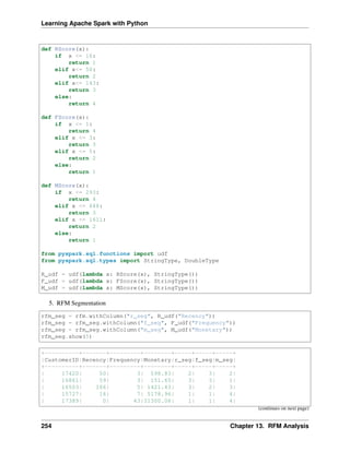
![Learning Apache Spark with Python
(continued from previous page)
+----------+-------+---------+--------+-----+-----+-----+
only showing top 5 rows
rfm_seg = rfm_seg.withColumn('RFMScore',
F.concat(F.col('r_seg'),F.col('f_seg'), F.col('m_
˓
→seg')))
rfm_seg.sort(F.col('RFMScore')).show(5)
+----------+-------+---------+--------+-----+-----+-----+--------+
|CustomerID|Recency|Frequency|Monetary|r_seg|f_seg|m_seg|RFMScore|
+----------+-------+---------+--------+-----+-----+-----+--------+
| 17988| 11| 8| 191.17| 1| 1| 1| 111|
| 16892| 1| 7| 496.84| 1| 1| 2| 112|
| 16668| 15| 6| 306.72| 1| 1| 2| 112|
| 16554| 3| 7| 641.55| 1| 1| 2| 112|
| 16500| 4| 6| 400.86| 1| 1| 2| 112|
+----------+-------+---------+--------+-----+-----+-----+--------+
only showing top 5 rows
13.2.3 Statistical Summary
6. Statistical Summary
• simple summary
rfm_seg.groupBy('RFMScore')
.agg({'Recency':'mean',
'Frequency': 'mean',
'Monetary': 'mean'} )
.sort(F.col('RFMScore')).show(5)
+--------+-----------------+------------------+------------------+
|RFMScore| avg(Recency)| avg(Monetary)| avg(Frequency)|
+--------+-----------------+------------------+------------------+
| 111| 11.0| 191.17| 8.0|
| 112| 8.0| 505.9775| 7.5|
| 113|7.237113402061856|1223.3604123711339| 7.752577319587629|
| 114|6.035123966942149| 8828.888595041324|18.882231404958677|
| 121| 9.6| 207.24| 4.4|
+--------+-----------------+------------------+------------------+
only showing top 5 rows
• complex summary
grp = 'RFMScore'
num_cols = ['Recency','Frequency','Monetary']
df_input = rfm_seg
quantile_grouped = quantile_agg(df_input,grp,num_cols)
(continues on next page)
13.2. Demo 255](https://image.slidesharecdn.com/pyspark-230429134708-b35c8a19/85/pyspark-pdf-261-320.jpg)
![Learning Apache Spark with Python
(continued from previous page)
quantile_grouped.toPandas().to_csv(output_dir+'quantile_grouped.csv')
deciles_grouped = deciles_agg(df_input,grp,num_cols)
deciles_grouped.toPandas().to_csv(output_dir+'deciles_grouped.csv')
13.3 Extension
You can also apply the K-means clustering in Clustering section to do the segmentation.
13.3.1 Build feature matrix
1. build dense feature matrix
from pyspark.sql import Row
from pyspark.ml.linalg import Vectors
# method 1 (good for small feature):
#def transData(row):
# return Row(label=row["Sales"],
# features=Vectors.dense([row["TV"],
# row["Radio"],
# row["Newspaper"]]))
# Method 2 (good for large features):
def transData(data):
return data.rdd.map(lambda r: [r[0],Vectors.dense(r[1:])]).toDF([
˓
→'CustomerID','rfm'])
transformed= transData(rfm)
transformed.show(5)
+----------+-------------------+
|CustomerID| rfm|
+----------+-------------------+
| 17420| [50.0,3.0,598.83]|
| 16861| [59.0,3.0,151.65]|
| 16503|[106.0,5.0,1421.43]|
| 15727| [16.0,7.0,5178.96]|
| 17389|[0.0,43.0,31300.08]|
+----------+-------------------+
only showing top 5 rows
2. Scaler the feature matrix
from pyspark.ml.feature import MinMaxScaler
scaler = MinMaxScaler(inputCol="rfm",
(continues on next page)
256 Chapter 13. RFM Analysis](https://image.slidesharecdn.com/pyspark-230429134708-b35c8a19/85/pyspark-pdf-262-320.jpg)
![Learning Apache Spark with Python
(continued from previous page)
outputCol="features")
scalerModel = scaler.fit(transformed)
scaledData = scalerModel.transform(transformed)
scaledData.show(5,False)
+----------+-------------------+----------------------------------------------
˓
→----------------+
|CustomerID|rfm |features
˓
→ |
+----------+-------------------+----------------------------------------------
˓
→----------------+
|17420 |[50.0,3.0,598.83] |[0.13404825737265416,0.008097165991902834,0.
˓
→01721938714830836]|
|16861 |[59.0,3.0,151.65] |[0.1581769436997319,0.008097165991902834,0.
˓
→01564357039241953] |
|16503 |[106.0,5.0,1421.43]|[0.28418230563002683,0.016194331983805668,0.
˓
→02011814573186342]|
|15727 |[16.0,7.0,5178.96] |[0.04289544235924933,0.024291497975708502,0.
˓
→03335929858922501]|
|17389 |[0.0,43.0,31300.08]|[0.0,0.1700404858299595,0.12540746393334334]
˓
→ |
+----------+-------------------+----------------------------------------------
˓
→----------------+
only showing top 5 rows
13.3.2 K-means clustering
3. Find optimal number of cluster
I will present two popular ways to determine the optimal number of the cluster.
• elbow analysis
#PySpark libraries
from pyspark.ml import Pipeline
from pyspark.ml.feature import StringIndexer, OneHotEncoder, VectorAssembler
from pyspark.sql.functions import col, percent_rank, lit
from pyspark.sql.window import Window
from pyspark.sql import DataFrame, Row
from pyspark.sql.types import StructType
from functools import reduce # For Python 3.x
from pyspark.ml.clustering import KMeans
#from pyspark.ml.evaluation import ClusteringEvaluator # requires Spark 2.4
˓
→or later
import numpy as np
cost = np.zeros(20)
for k in range(2,20):
kmeans = KMeans()
(continues on next page)
13.3. Extension 257](https://image.slidesharecdn.com/pyspark-230429134708-b35c8a19/85/pyspark-pdf-263-320.jpg)
![Learning Apache Spark with Python
(continued from previous page)
.setK(k)
.setSeed(1)
.setFeaturesCol("features")
.setPredictionCol("cluster")
model = kmeans.fit(scaledData)
cost[k] = model.computeCost(scaledData) # requires Spark 2.0 or later
import numpy as np
import matplotlib.mlab as mlab
import matplotlib.pyplot as plt
import seaborn as sbs
from matplotlib.ticker import MaxNLocator
fig, ax = plt.subplots(1,1, figsize =(8,6))
ax.plot(range(2,20),cost[2:20], marker = "o")
ax.set_xlabel('k')
ax.set_ylabel('cost')
ax.xaxis.set_major_locator(MaxNLocator(integer=True))
plt.show()
258 Chapter 13. RFM Analysis](https://image.slidesharecdn.com/pyspark-230429134708-b35c8a19/85/pyspark-pdf-264-320.jpg)
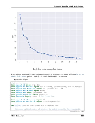
![Learning Apache Spark with Python
(continued from previous page)
:param df_in: the input dataframe
:param index_col: the name of the index column
:param k_min: the train dataset
:param k_min: the minmum number of the clusters
:param k_max: the maxmum number of the clusters
:param num_runs: the number of runs for each fixed clusters
:return k: optimal number of the clusters
:return silh_lst: Silhouette score
:return r_table: the running results table
:author: Wenqiang Feng
:email: von198@gmail.com.com
'''
start = time.time()
silh_lst = []
k_lst = np.arange(k_min, k_max+1)
r_table = df_in.select(index_col).toPandas()
r_table = r_table.set_index(index_col)
centers = pd.DataFrame()
for k in k_lst:
silh_val = []
for run in np.arange(1, num_runs+1):
# Trains a k-means model.
kmeans = KMeans()
.setK(k)
.setSeed(int(np.random.randint(100, size=1)))
model = kmeans.fit(df_in)
# Make predictions
predictions = model.transform(df_in)
r_table['cluster_{k}_{run}'.format(k=k, run=run)]= predictions.
˓
→select('prediction').toPandas()
# Evaluate clustering by computing Silhouette score
evaluator = ClusteringEvaluator()
silhouette = evaluator.evaluate(predictions)
silh_val.append(silhouette)
silh_array=np.asanyarray(silh_val)
silh_lst.append(silh_array.mean())
elapsed = time.time() - start
silhouette = pd.DataFrame(list(zip(k_lst,silh_lst)),columns = ['k',
˓
→'silhouette'])
print('+------------------------------------------------------------+')
(continues on next page)
260 Chapter 13. RFM Analysis](https://image.slidesharecdn.com/pyspark-230429134708-b35c8a19/85/pyspark-pdf-266-320.jpg)
![Learning Apache Spark with Python
(continued from previous page)
print("| The finding optimal k phase took %8.0f s. |"
˓
→%(elapsed))
print('+------------------------------------------------------------+')
return k_lst[np.argmax(silh_lst, axis=0)], silhouette , r_table
k, silh_lst, r_table = optimal_k(scaledData,index_col,k_min, k_max,num_runs)
+------------------------------------------------------------+
| The finding optimal k phase took 1783 s. |
+------------------------------------------------------------+
spark.createDataFrame(silh_lst).show()
+---+------------------+
| k| silhouette|
+---+------------------+
| 3|0.8045154385557953|
| 4|0.6993528775512052|
| 5|0.6689286654221447|
| 6|0.6356184024841809|
| 7|0.7174102265711756|
| 8|0.6720861758298997|
| 9| 0.601771359881241|
| 10|0.6292447334578428|
+---+------------------+
From the silhouette list, we can choose 3 as the optimal number of the clusters.
Warning: ClusteringEvaluator in pyspark.ml.evaluation requires Spark 2.4 or later!!
4. K-means clustering
k = 3
kmeans = KMeans().setK(k).setSeed(1)
model = kmeans.fit(scaledData)
# Make predictions
predictions = model.transform(scaledData)
predictions.show(5,False)
+----------+-------------------+--------------------+----------+
|CustomerID| rfm| features|prediction|
+----------+-------------------+--------------------+----------+
| 17420| [50.0,3.0,598.83]|[0.13404825737265...| 0|
| 16861| [59.0,3.0,151.65]|[0.15817694369973...| 0|
| 16503|[106.0,5.0,1421.43]|[0.28418230563002...| 2|
| 15727| [16.0,7.0,5178.96]|[0.04289544235924...| 0|
| 17389|[0.0,43.0,31300.08]|[0.0,0.1700404858...| 0|
(continues on next page)
13.3. Extension 261](https://image.slidesharecdn.com/pyspark-230429134708-b35c8a19/85/pyspark-pdf-267-320.jpg)
![Learning Apache Spark with Python
(continued from previous page)
+----------+-------------------+--------------------+----------+
only showing top 5 rows
13.3.3 Statistical summary
5. statistical summary
results = rfm.join(predictions.select('CustomerID','prediction'),'CustomerID',
˓
→how='left')
results.show(5)
+----------+-------+---------+--------+----------+
|CustomerID|Recency|Frequency|Monetary|prediction|
+----------+-------+---------+--------+----------+
| 13098| 1| 41|28658.88| 0|
| 13248| 124| 2| 465.68| 2|
| 13452| 259| 2| 590.0| 1|
| 13460| 29| 2| 183.44| 0|
| 13518| 85| 1| 659.44| 0|
+----------+-------+---------+--------+----------+
only showing top 5 rows
• simple summary
results.groupBy('prediction')
.agg({'Recency':'mean',
'Frequency': 'mean',
'Monetary': 'mean'} )
.sort(F.col('prediction')).show(5)
+----------+------------------+------------------+------------------+
|prediction| avg(Recency)| avg(Monetary)| avg(Frequency)|
+----------+------------------+------------------+------------------+
| 0|30.966337980278816|2543.0355321319284| 6.514450867052023|
| 1|296.02403846153845|407.16831730769206|1.5592948717948718|
| 2|154.40148698884758| 702.5096406443623| 2.550185873605948|
+----------+------------------+------------------+------------------+
• complex summary
grp = 'RFMScore'
num_cols = ['Recency','Frequency','Monetary']
df_input = results
quantile_grouped = quantile_agg(df_input,grp,num_cols)
quantile_grouped.toPandas().to_csv(output_dir+'quantile_grouped.csv')
deciles_grouped = deciles_agg(df_input,grp,num_cols)
deciles_grouped.toPandas().to_csv(output_dir+'deciles_grouped.csv')
262 Chapter 13. RFM Analysis](https://image.slidesharecdn.com/pyspark-230429134708-b35c8a19/85/pyspark-pdf-268-320.jpg)
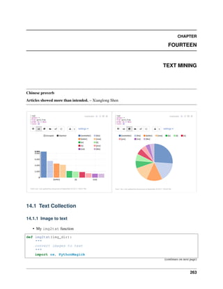
![Learning Apache Spark with Python
(continued from previous page)
from datetime import datetime
import PyPDF2
from PIL import Image
import pytesseract
f = open('doc4img.txt','wa')
for img in [img_file for img_file in os.listdir(img_dir)
if (img_file.endswith(".png") or
img_file.endswith(".jpg") or
img_file.endswith(".jpeg"))]:
start_time = datetime.now()
input_img = img_dir + "/" + img
print('---------------------------------------------------------------
˓
→-----')
print(img)
print('Converting ' + img +'.......')
print('---------------------------------------------------------------
˓
→-----')
# extract the text information from images
text = pytesseract.image_to_string(Image.open(input_img))
print(text)
# ouput text file
f.write( img + "n")
f.write(text.encode('utf-8'))
print "CPU Time for converting" + img +":"+ str(datetime.now() -
˓
→start_time) +"n"
f.write( "n----------------------------------------------------------
˓
→---n")
f.close()
• Demo
I applied my img2txt function to the image in Image folder.
image_dir = r"Image"
img2txt(image_dir)
Then I got the following results:
--------------------------------------------------------------------
feng.pdf_0.png
Converting feng.pdf_0.png.......
(continues on next page)
264 Chapter 14. Text Mining](https://image.slidesharecdn.com/pyspark-230429134708-b35c8a19/85/pyspark-pdf-270-320.jpg)
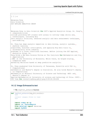
![Learning Apache Spark with Python
(continued from previous page)
from PIL import Image, ImageEnhance, ImageFilter
import pytesseract
f = open('doc4img.txt','wa')
for img in [img_file for img_file in os.listdir(img_dir)
if (img_file.endswith(".png") or
img_file.endswith(".jpg") or
img_file.endswith(".jpeg"))]:
start_time = datetime.now()
input_img = img_dir + "/" + img
enhanced_img = img_dir + "/" +"Enhanced" + "/"+ img
im = Image.open(input_img) # the second one
im = im.filter(ImageFilter.MedianFilter())
enhancer = ImageEnhance.Contrast(im)
im = enhancer.enhance(1)
im = im.convert('1')
im.save(enhanced_img)
for scale in np.ones(scaler):
im = Image.open(enhanced_img) # the second one
im = im.filter(ImageFilter.MedianFilter())
enhancer = ImageEnhance.Contrast(im)
im = enhancer.enhance(scale)
im = im.convert('1')
im.save(enhanced_img)
print('---------------------------------------------------------------
˓
→-----')
print(img)
print('Converting ' + img +'.......')
print('---------------------------------------------------------------
˓
→-----')
# extract the text information from images
text = pytesseract.image_to_string(Image.open(enhanced_img))
print(text)
# ouput text file
f.write( img + "n")
f.write(text.encode('utf-8'))
print "CPU Time for converting" + img +":"+ str(datetime.now() -
˓
→start_time) +"n"
f.write( "n----------------------------------------------------------
˓
→---n")
(continues on next page)
266 Chapter 14. Text Mining](https://image.slidesharecdn.com/pyspark-230429134708-b35c8a19/85/pyspark-pdf-272-320.jpg)
![Learning Apache Spark with Python
(continued from previous page)
from PIL import Image
import pytesseract
f = open('doc.txt','wa')
for pdf in [pdf_file for pdf_file in os.listdir(pdf_dir) if pdf_file.
˓
→endswith(".pdf")]:
start_time = datetime.now()
input_pdf = pdf_dir + "/" + pdf
pdf_im = PyPDF2.PdfFileReader(file(input_pdf, "rb"))
npage = pdf_im.getNumPages()
print('---------------------------------------------------------------
˓
→-----')
print(pdf)
print('Converting %d pages.' % npage)
print('---------------------------------------------------------------
˓
→-----')
f.write( "n----------------------------------------------------------
˓
→----------n")
for p in range(npage):
pdf_file = input_pdf + '[' + str(p) +']'
image_file = image_dir + "/" + pdf+ '_' + str(p)+ '.png'
# convert PDF files to Images
im = PythonMagick.Image()
im.density('300')
im.read(pdf_file)
im.write(image_file)
# extract the text information from images
text = pytesseract.image_to_string(Image.open(image_file))
#print(text)
# ouput text file
f.write( pdf + "n")
f.write(text.encode('utf-8'))
print "CPU Time for converting" + pdf +":"+ str(datetime.now() -
˓
→start_time) +"n"
f.close()
• Demo
268 Chapter 14. Text Mining](https://image.slidesharecdn.com/pyspark-230429134708-b35c8a19/85/pyspark-pdf-274-320.jpg)
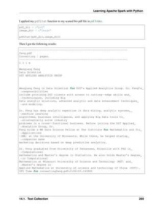
![Learning Apache Spark with Python
14.1.4 Audio to text
• My audio2txt function
def audio2txt(audio_dir):
''' convert audio to text'''
import speech_recognition as sr
r = sr.Recognizer()
f = open('doc.txt','wa')
for audio_n in [audio_file for audio_file in os.listdir(audio_dir)
if audio_file.endswith(".wav")]:
filename = audio_dir + "/" + audio_n
# Read audio data
with sr.AudioFile(filename) as source:
audio = r.record(source) # read the entire audio file
# Google Speech Recognition
text = r.recognize_google(audio)
# ouput text file
f.write( audio_n + ": ")
f.write(text.encode('utf-8'))
f.write("n")
print('You said: ' + text)
f.close()
• Demo
I applied my audio2txt function to my audio records in audio folder.
audio_dir = r"audio"
audio2txt(audio_dir)
Then I got the following results:
You said: hello this is George welcome to my tutorial
You said: mathematics is important in daily life
You said: call me tomorrow
You said: do you want something to eat
You said: I want to speak with him
You said: nice to see you
You said: can you speak slowly
You said: have a good day
By the way, you can use my following python code to record your own audio and play with audio2txt
function in Command-line python record.py "demo2.wav":
270 Chapter 14. Text Mining](https://image.slidesharecdn.com/pyspark-230429134708-b35c8a19/85/pyspark-pdf-276-320.jpg)
![Learning Apache Spark with Python
import sys, getopt
import speech_recognition as sr
audio_filename = sys.argv[1]
r = sr.Recognizer()
with sr.Microphone() as source:
r.adjust_for_ambient_noise(source)
print("Hey there, say something, I am recording!")
audio = r.listen(source)
print("Done listening!")
with open(audio_filename, "wb") as f:
f.write(audio.get_wav_data())
14.2 Text Preprocessing
• check to see if a row only contains whitespace
def check_blanks(data_str):
is_blank = str(data_str.isspace())
return is_blank
• Determine whether the language of the text content is english or not: Use langid module to classify
the language to make sure we are applying the correct cleanup actions for English langid
def check_lang(data_str):
predict_lang = langid.classify(data_str)
if predict_lang[1] >= .9:
language = predict_lang[0]
else:
language = 'NA'
return language
• Remove features
def remove_features(data_str):
# compile regex
url_re = re.compile('https?://(www.)?w+.w+(/w+)*/?')
punc_re = re.compile('[%s]' % re.escape(string.punctuation))
num_re = re.compile('(d+)')
mention_re = re.compile('@(w+)')
alpha_num_re = re.compile("^[a-z0-9_.]+$")
# convert to lowercase
data_str = data_str.lower()
# remove hyperlinks
data_str = url_re.sub(' ', data_str)
# remove @mentions
data_str = mention_re.sub(' ', data_str)
(continues on next page)
14.2. Text Preprocessing 271](https://image.slidesharecdn.com/pyspark-230429134708-b35c8a19/85/pyspark-pdf-277-320.jpg)
![Learning Apache Spark with Python
(continued from previous page)
# remove puncuation
data_str = punc_re.sub(' ', data_str)
# remove numeric 'words'
data_str = num_re.sub(' ', data_str)
# remove non a-z 0-9 characters and words shorter than 3 characters
list_pos = 0
cleaned_str = ''
for word in data_str.split():
if list_pos == 0:
if alpha_num_re.match(word) and len(word) > 2:
cleaned_str = word
else:
cleaned_str = ' '
else:
if alpha_num_re.match(word) and len(word) > 2:
cleaned_str = cleaned_str + ' ' + word
else:
cleaned_str += ' '
list_pos += 1
return cleaned_str
• removes stop words
def remove_stops(data_str):
# expects a string
stops = set(stopwords.words("english"))
list_pos = 0
cleaned_str = ''
text = data_str.split()
for word in text:
if word not in stops:
# rebuild cleaned_str
if list_pos == 0:
cleaned_str = word
else:
cleaned_str = cleaned_str + ' ' + word
list_pos += 1
return cleaned_str
• tagging text
def tag_and_remove(data_str):
cleaned_str = ' '
# noun tags
nn_tags = ['NN', 'NNP', 'NNP', 'NNPS', 'NNS']
# adjectives
jj_tags = ['JJ', 'JJR', 'JJS']
# verbs
vb_tags = ['VB', 'VBD', 'VBG', 'VBN', 'VBP', 'VBZ']
nltk_tags = nn_tags + jj_tags + vb_tags
(continues on next page)
272 Chapter 14. Text Mining](https://image.slidesharecdn.com/pyspark-230429134708-b35c8a19/85/pyspark-pdf-278-320.jpg)
![Learning Apache Spark with Python
(continued from previous page)
# break string into 'words'
text = data_str.split()
# tag the text and keep only those with the right tags
tagged_text = pos_tag(text)
for tagged_word in tagged_text:
if tagged_word[1] in nltk_tags:
cleaned_str += tagged_word[0] + ' '
return cleaned_str
• lemmatization
def lemmatize(data_str):
# expects a string
list_pos = 0
cleaned_str = ''
lmtzr = WordNetLemmatizer()
text = data_str.split()
tagged_words = pos_tag(text)
for word in tagged_words:
if 'v' in word[1].lower():
lemma = lmtzr.lemmatize(word[0], pos='v')
else:
lemma = lmtzr.lemmatize(word[0], pos='n')
if list_pos == 0:
cleaned_str = lemma
else:
cleaned_str = cleaned_str + ' ' + lemma
list_pos += 1
return cleaned_str
define the preprocessing function in PySpark
from pyspark.sql.functions import udf
from pyspark.sql.types import StringType
import preproc as pp
check_lang_udf = udf(pp.check_lang, StringType())
remove_stops_udf = udf(pp.remove_stops, StringType())
remove_features_udf = udf(pp.remove_features, StringType())
tag_and_remove_udf = udf(pp.tag_and_remove, StringType())
lemmatize_udf = udf(pp.lemmatize, StringType())
check_blanks_udf = udf(pp.check_blanks, StringType())
14.2. Text Preprocessing 273](https://image.slidesharecdn.com/pyspark-230429134708-b35c8a19/85/pyspark-pdf-279-320.jpg)
![Learning Apache Spark with Python
14.3 Text Classification
Theoretically speaking, you may apply any classification algorithms to do classification. I will only present
Naive Bayes method is the following.
14.3.1 Introduction
14.3.2 Demo
1. create spark contexts
import pyspark
from pyspark.sql import SQLContext
# create spark contexts
sc = pyspark.SparkContext()
sqlContext = SQLContext(sc)
2. load dataset
# Load a text file and convert each line to a Row.
data_rdd = sc.textFile("../data/raw_data.txt")
parts_rdd = data_rdd.map(lambda l: l.split("t"))
# Filter bad rows out
garantee_col_rdd = parts_rdd.filter(lambda l: len(l) == 3)
typed_rdd = garantee_col_rdd.map(lambda p: (p[0], p[1], float(p[2])))
#Create DataFrame
data_df = sqlContext.createDataFrame(typed_rdd, ["text", "id", "label"])
# get the raw columns
raw_cols = data_df.columns
#data_df.show()
data_df.printSchema()
274 Chapter 14. Text Mining](https://image.slidesharecdn.com/pyspark-230429134708-b35c8a19/85/pyspark-pdf-280-320.jpg)
![Learning Apache Spark with Python
root
|-- text: string (nullable = true)
|-- id: string (nullable = true)
|-- label: double (nullable = true)
+--------------------+------------------+-----+
| text| id|label|
+--------------------+------------------+-----+
|Fresh install of ...| 1018769417| 1.0|
|Well. Now I know ...| 10284216536| 1.0|
|"Literally six we...| 10298589026| 1.0|
|Mitsubishi i MiEV...|109017669432377344| 1.0|
+--------------------+------------------+-----+
only showing top 4 rows
3. setup pyspark udf function
from pyspark.sql.functions import udf
from pyspark.sql.types import StringType
import preproc as pp
# Register all the functions in Preproc with Spark Context
check_lang_udf = udf(pp.check_lang, StringType())
remove_stops_udf = udf(pp.remove_stops, StringType())
remove_features_udf = udf(pp.remove_features, StringType())
tag_and_remove_udf = udf(pp.tag_and_remove, StringType())
lemmatize_udf = udf(pp.lemmatize, StringType())
check_blanks_udf = udf(pp.check_blanks, StringType())
4. language identification
lang_df = data_df.withColumn("lang", check_lang_udf(data_df["text"]))
en_df = lang_df.filter(lang_df["lang"] == "en")
en_df.show(4)
+--------------------+------------------+-----+----+
| text| id|label|lang|
+--------------------+------------------+-----+----+
|RT @goeentertain:...|665305154954989568| 1.0| en|
|Teforia Uses Mach...|660668007975268352| 1.0| en|
| Apple TV or Roku?| 25842461136| 1.0| en|
|Finished http://t...| 9412369614| 1.0| en|
+--------------------+------------------+-----+----+
only showing top 4 rows
5. remove stop words
rm_stops_df = en_df.select(raw_cols)
.withColumn("stop_text", remove_stops_udf(en_df["text"]))
rm_stops_df.show(4)
14.3. Text Classification 275](https://image.slidesharecdn.com/pyspark-230429134708-b35c8a19/85/pyspark-pdf-281-320.jpg)
![Learning Apache Spark with Python
+--------------------+------------------+-----+--------------------+
| text| id|label| stop_text|
+--------------------+------------------+-----+--------------------+
|RT @goeentertain:...|665305154954989568| 1.0|RT @goeentertain:...|
|Teforia Uses Mach...|660668007975268352| 1.0|Teforia Uses Mach...|
| Apple TV or Roku?| 25842461136| 1.0| Apple TV Roku?|
|Finished http://t...| 9412369614| 1.0|Finished http://t...|
+--------------------+------------------+-----+--------------------+
only showing top 4 rows
6. remove irrelevant features
rm_features_df = rm_stops_df.select(raw_cols+["stop_text"])
.withColumn("feat_text",
remove_features_udf(rm_stops_df["stop_text"]))
rm_features_df.show(4)
+--------------------+------------------+-----+--------------------+----------
˓
→----------+
| text| id|label| stop_text|
˓
→ feat_text|
+--------------------+------------------+-----+--------------------+----------
˓
→----------+
|RT @goeentertain:...|665305154954989568| 1.0|RT @goeentertain:...| future
˓
→blase ...|
|Teforia Uses Mach...|660668007975268352| 1.0|Teforia Uses Mach...|teforia
˓
→uses mach...|
| Apple TV or Roku?| 25842461136| 1.0| Apple TV Roku?|
˓
→apple roku|
|Finished http://t...| 9412369614| 1.0|Finished http://t...|
˓
→ finished|
+--------------------+------------------+-----+--------------------+----------
˓
→----------+
only showing top 4 rows
7. tag the words
tagged_df = rm_features_df.select(raw_cols+["feat_text"])
.withColumn("tagged_text",
tag_and_remove_udf(rm_features_df.feat_text))
tagged_df.show(4)
+--------------------+------------------+-----+--------------------+----------
˓
→----------+
| text| id|label| feat_text|
˓
→tagged_text|
+--------------------+------------------+-----+--------------------+----------
˓
→----------+
|RT @goeentertain:...|665305154954989568| 1.0| future blase ...| future
˓
→blase vic...|
(continues on next page)
276 Chapter 14. Text Mining](https://image.slidesharecdn.com/pyspark-230429134708-b35c8a19/85/pyspark-pdf-282-320.jpg)
![Learning Apache Spark with Python
(continued from previous page)
|Teforia Uses Mach...|660668007975268352| 1.0|teforia uses mach...| teforia
˓
→uses mac...|
| Apple TV or Roku?| 25842461136| 1.0| apple roku|
˓
→apple roku |
|Finished http://t...| 9412369614| 1.0| finished|
˓
→ finished |
+--------------------+------------------+-----+--------------------+----------
˓
→----------+
only showing top 4 rows
8. lemmatization of words
lemm_df = tagged_df.select(raw_cols+["tagged_text"])
.withColumn("lemm_text", lemmatize_udf(tagged_df["tagged_
˓
→text"]))
lemm_df.show(4)
+--------------------+------------------+-----+--------------------+----------
˓
→----------+
| text| id|label| tagged_text|
˓
→ lemm_text|
+--------------------+------------------+-----+--------------------+----------
˓
→----------+
|RT @goeentertain:...|665305154954989568| 1.0| future blase vic...|future
˓
→blase vice...|
|Teforia Uses Mach...|660668007975268352| 1.0| teforia uses mac...|teforia
˓
→use machi...|
| Apple TV or Roku?| 25842461136| 1.0| apple roku |
˓
→apple roku|
|Finished http://t...| 9412369614| 1.0| finished |
˓
→ finish|
+--------------------+------------------+-----+--------------------+----------
˓
→----------+
only showing top 4 rows
9. remove blank rows and drop duplicates
check_blanks_df = lemm_df.select(raw_cols+["lemm_text"])
.withColumn("is_blank", check_blanks_udf(lemm_df[
˓
→"lemm_text"]))
# remove blanks
no_blanks_df = check_blanks_df.filter(check_blanks_df["is_blank"] ==
˓
→"False")
# drop duplicates
dedup_df = no_blanks_df.dropDuplicates(['text', 'label'])
dedup_df.show(4)
+--------------------+------------------+-----+--------------------+--------+
| text| id|label| lemm_text|is_blank|
(continues on next page)
14.3. Text Classification 277](https://image.slidesharecdn.com/pyspark-230429134708-b35c8a19/85/pyspark-pdf-283-320.jpg)
![Learning Apache Spark with Python
# Split the data into training and test sets (40% held out for testing)
(trainingData, testData) = data.randomSplit([0.6, 0.4])
13. NaiveBayes Pipeline
from pyspark.ml.feature import HashingTF, IDF, Tokenizer
from pyspark.ml import Pipeline
from pyspark.ml.classification import NaiveBayes, RandomForestClassifier
from pyspark.ml.classification import DecisionTreeClassifier
from pyspark.ml.evaluation import MulticlassClassificationEvaluator
from pyspark.ml.tuning import ParamGridBuilder
from pyspark.ml.tuning import CrossValidator
from pyspark.ml.feature import IndexToString, StringIndexer, VectorIndexer
from pyspark.ml.feature import CountVectorizer
# Configure an ML pipeline, which consists of tree stages: tokenizer,
˓
→hashingTF, and nb.
tokenizer = Tokenizer(inputCol="text", outputCol="words")
hashingTF = HashingTF(inputCol=tokenizer.getOutputCol(), outputCol=
˓
→"rawFeatures")
# vectorizer = CountVectorizer(inputCol= "words", outputCol="rawFeatures")
idf = IDF(minDocFreq=3, inputCol="rawFeatures", outputCol="features")
# Naive Bayes model
nb = NaiveBayes()
# Pipeline Architecture
pipeline = Pipeline(stages=[tokenizer, hashingTF, idf, nb])
# Train model. This also runs the indexers.
model = pipeline.fit(trainingData)
14. Make predictions
predictions = model.transform(testData)
# Select example rows to display.
predictions.select("text", "label", "prediction").show(5,False)
+-----------------------------------------------+-----+----------+
|text |label|prediction|
+-----------------------------------------------+-----+----------+
|finish |1.0 |1.0 |
|meet rolo dogsofthinkgeek happy nationaldogday |1.0 |1.0 |
|pumpkin family |1.0 |1.0 |
|meet jet dogsofthinkgeek happy nationaldogday |1.0 |1.0 |
|meet vixie dogsofthinkgeek happy nationaldogday|1.0 |1.0 |
+-----------------------------------------------+-----+----------+
only showing top 5 rows
15. evaluation
14.3. Text Classification 279](https://image.slidesharecdn.com/pyspark-230429134708-b35c8a19/85/pyspark-pdf-285-320.jpg)
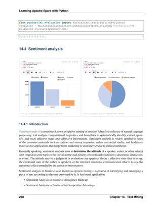
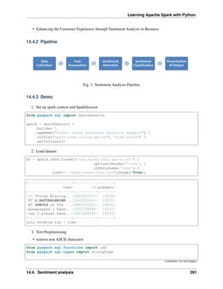
![Learning Apache Spark with Python
(continued from previous page)
from nltk.stem.wordnet import WordNetLemmatizer
from nltk.corpus import stopwords
from nltk import pos_tag
import string
import re
# remove non ASCII characters
def strip_non_ascii(data_str):
''' Returns the string without non ASCII characters'''
stripped = (c for c in data_str if 0 < ord(c) < 127)
return ''.join(stripped)
# setup pyspark udf function
strip_non_ascii_udf = udf(strip_non_ascii, StringType())
check:
df = df.withColumn('text_non_asci',strip_non_ascii_udf(df['text']))
df.show(5,True)
ouput:
+--------------------+----------+-------+--------------------+
| text| id|pubdate| text_non_asci|
+--------------------+----------+-------+--------------------+
|10 Things Missing...|2602860537| 18536|10 Things Missing...|
|RT @_NATURALBWINN...|2602850443| 18536|RT @_NATURALBWINN...|
|RT @HBO24 yo the ...|2602761852| 18535|RT @HBO24 yo the ...|
|Aaaaaaaand I have...|2602738438| 18535|Aaaaaaaand I have...|
|can I please have...|2602684185| 18535|can I please have...|
+--------------------+----------+-------+--------------------+
only showing top 5 rows
• fixed abbreviation
# fixed abbreviation
def fix_abbreviation(data_str):
data_str = data_str.lower()
data_str = re.sub(r'bthatsb', 'that is', data_str)
data_str = re.sub(r'biveb', 'i have', data_str)
data_str = re.sub(r'bimb', 'i am', data_str)
data_str = re.sub(r'byab', 'yeah', data_str)
data_str = re.sub(r'bcantb', 'can not', data_str)
data_str = re.sub(r'bdontb', 'do not', data_str)
data_str = re.sub(r'bwontb', 'will not', data_str)
data_str = re.sub(r'bidb', 'i would', data_str)
data_str = re.sub(r'wtf', 'what the fuck', data_str)
data_str = re.sub(r'bwthb', 'what the hell', data_str)
data_str = re.sub(r'brb', 'are', data_str)
data_str = re.sub(r'bub', 'you', data_str)
data_str = re.sub(r'bkb', 'OK', data_str)
data_str = re.sub(r'bsuxb', 'sucks', data_str)
(continues on next page)
282 Chapter 14. Text Mining](https://image.slidesharecdn.com/pyspark-230429134708-b35c8a19/85/pyspark-pdf-288-320.jpg)
![Learning Apache Spark with Python
(continued from previous page)
data_str = re.sub(r'bno+b', 'no', data_str)
data_str = re.sub(r'bcoo+b', 'cool', data_str)
data_str = re.sub(r'rtb', '', data_str)
data_str = data_str.strip()
return data_str
fix_abbreviation_udf = udf(fix_abbreviation, StringType())
check:
df = df.withColumn('fixed_abbrev',fix_abbreviation_udf(df['text_non_asci
˓
→']))
df.show(5,True)
ouput:
+--------------------+----------+-------+--------------------+----------------
˓
→----+
| text| id|pubdate| text_non_asci| fixed_
˓
→abbrev|
+--------------------+----------+-------+--------------------+----------------
˓
→----+
|10 Things Missing...|2602860537| 18536|10 Things Missing...|10 things
˓
→missing...|
|RT @_NATURALBWINN...|2602850443| 18536|RT @_NATURALBWINN...|@_
˓
→naturalbwinner ...|
|RT @HBO24 yo the ...|2602761852| 18535|RT @HBO24 yo the ...|@hbo24 yo the
˓
→#ne...|
|Aaaaaaaand I have...|2602738438| 18535|Aaaaaaaand I have...|aaaaaaaand i
˓
→have...|
|can I please have...|2602684185| 18535|can I please have...|can i please
˓
→have...|
+--------------------+----------+-------+--------------------+----------------
˓
→----+
only showing top 5 rows
• remove irrelevant features
def remove_features(data_str):
# compile regex
url_re = re.compile('https?://(www.)?w+.w+(/w+)*/?')
punc_re = re.compile('[%s]' % re.escape(string.punctuation))
num_re = re.compile('(d+)')
mention_re = re.compile('@(w+)')
alpha_num_re = re.compile("^[a-z0-9_.]+$")
# convert to lowercase
data_str = data_str.lower()
# remove hyperlinks
data_str = url_re.sub(' ', data_str)
# remove @mentions
data_str = mention_re.sub(' ', data_str)
(continues on next page)
14.4. Sentiment analysis 283](https://image.slidesharecdn.com/pyspark-230429134708-b35c8a19/85/pyspark-pdf-289-320.jpg)
![Learning Apache Spark with Python
(continued from previous page)
# remove puncuation
data_str = punc_re.sub(' ', data_str)
# remove numeric 'words'
data_str = num_re.sub(' ', data_str)
# remove non a-z 0-9 characters and words shorter than 1 characters
list_pos = 0
cleaned_str = ''
for word in data_str.split():
if list_pos == 0:
if alpha_num_re.match(word) and len(word) > 1:
cleaned_str = word
else:
cleaned_str = ' '
else:
if alpha_num_re.match(word) and len(word) > 1:
cleaned_str = cleaned_str + ' ' + word
else:
cleaned_str += ' '
list_pos += 1
# remove unwanted space, *.split() will automatically split on
# whitespace and discard duplicates, the " ".join() joins the
# resulting list into one string.
return " ".join(cleaned_str.split())
# setup pyspark udf function
remove_features_udf = udf(remove_features, StringType())
check:
df = df.withColumn('removed',remove_features_udf(df['fixed_abbrev']))
df.show(5,True)
ouput:
+--------------------+----------+-------+--------------------+----------------
˓
→----+--------------------+
| text| id|pubdate| text_non_asci| fixed_
˓
→abbrev| removed|
+--------------------+----------+-------+--------------------+----------------
˓
→----+--------------------+
|10 Things Missing...|2602860537| 18536|10 Things Missing...|10 things
˓
→missing...|things missing in...|
|RT @_NATURALBWINN...|2602850443| 18536|RT @_NATURALBWINN...|@_
˓
→naturalbwinner ...|oh and do not lik...|
|RT @HBO24 yo the ...|2602761852| 18535|RT @HBO24 yo the ...|@hbo24 yo the
˓
→#ne...|yo the newtwitter...|
|Aaaaaaaand I have...|2602738438| 18535|Aaaaaaaand I have...|aaaaaaaand i
˓
→have...|aaaaaaaand have t...|
|can I please have...|2602684185| 18535|can I please have...|can i please
˓
→have...|can please have t...|
+--------------------+----------+-------+--------------------+----------------
˓
→----+--------------------+
only showing top 5 rows
284 Chapter 14. Text Mining](https://image.slidesharecdn.com/pyspark-230429134708-b35c8a19/85/pyspark-pdf-290-320.jpg)
![Learning Apache Spark with Python
4. Sentiment Analysis main function
from pyspark.sql.types import FloatType
from textblob import TextBlob
def sentiment_analysis(text):
return TextBlob(text).sentiment.polarity
sentiment_analysis_udf = udf(sentiment_analysis , FloatType())
df = df.withColumn("sentiment_score", sentiment_analysis_udf( df['removed']
˓
→))
df.show(5,True)
• Sentiment score
+--------------------+---------------+
| removed|sentiment_score|
+--------------------+---------------+
|things missing in...| -0.03181818|
|oh and do not lik...| -0.03181818|
|yo the newtwitter...| 0.3181818|
|aaaaaaaand have t...| 0.11818182|
|can please have t...| 0.13636364|
+--------------------+---------------+
only showing top 5 rows
• Words frequency
• Sentiment Classification
14.4. Sentiment analysis 285](https://image.slidesharecdn.com/pyspark-230429134708-b35c8a19/85/pyspark-pdf-291-320.jpg)
![Learning Apache Spark with Python
14.6.2 Demo
1. Load data
rawdata = spark.read.load("../data/airlines.csv", format="csv",
˓
→header=True)
rawdata.show(5)
+-----+---------------+---------+--------+------+--------+-----+-----
˓
→------+--------------------+
| id| airline| date|location|rating|
˓
→cabin|value|recommended| review|
+-----+---------------+---------+--------+------+--------+-----+-----
˓
→------+--------------------+
|10001|Delta Air Lines|21-Jun-14|Thailand| 7| Economy| 4|
˓
→ YES|Flew Mar 30 NRT t...|
|10002|Delta Air Lines|19-Jun-14| USA| 0| Economy| 2|
˓
→ NO|Flight 2463 leavi...|
|10003|Delta Air Lines|18-Jun-14| USA| 0| Economy| 1|
˓
→ NO|Delta Website fro...|
|10004|Delta Air Lines|17-Jun-14| USA| 9|Business| 4|
˓
→ YES|"I just returned ...|
|10005|Delta Air Lines|17-Jun-14| Ecuador| 7| Economy| 3|
˓
→ YES|"Round-trip fligh...|
+-----+---------------+---------+--------+------+--------+-----+-----
˓
→------+--------------------+
only showing top 5 rows
1. Text preprocessing
I will use the following raw column names to keep my table concise:
raw_cols = rawdata.columns
raw_cols
['id', 'airline', 'date', 'location', 'rating', 'cabin', 'value',
˓
→'recommended', 'review']
rawdata = rawdata.dropDuplicates(['review'])
from pyspark.sql.functions import udf, col
from pyspark.sql.types import StringType, DoubleType, DateType
from nltk.stem.wordnet import WordNetLemmatizer
from nltk.corpus import stopwords
from nltk import pos_tag
import langid
import string
import re
• remove non ASCII characters
288 Chapter 14. Text Mining](https://image.slidesharecdn.com/pyspark-230429134708-b35c8a19/85/pyspark-pdf-294-320.jpg)
![Learning Apache Spark with Python
# remove non ASCII characters
def strip_non_ascii(data_str):
''' Returns the string without non ASCII characters'''
stripped = (c for c in data_str if 0 < ord(c) < 127)
return ''.join(stripped)
• check it blank line or not
# check to see if a row only contains whitespace
def check_blanks(data_str):
is_blank = str(data_str.isspace())
return is_blank
• check the language (a little bit slow, I skited this step)
# check the language (only apply to english)
def check_lang(data_str):
from langid.langid import LanguageIdentifier, model
identifier = LanguageIdentifier.from_modelstring(model, norm_
˓
→probs=True)
predict_lang = identifier.classify(data_str)
if predict_lang[1] >= .9:
language = predict_lang[0]
else:
language = predict_lang[0]
return language
• fixed abbreviation
# fixed abbreviation
def fix_abbreviation(data_str):
data_str = data_str.lower()
data_str = re.sub(r'bthatsb', 'that is', data_str)
data_str = re.sub(r'biveb', 'i have', data_str)
data_str = re.sub(r'bimb', 'i am', data_str)
data_str = re.sub(r'byab', 'yeah', data_str)
data_str = re.sub(r'bcantb', 'can not', data_str)
data_str = re.sub(r'bdontb', 'do not', data_str)
data_str = re.sub(r'bwontb', 'will not', data_str)
data_str = re.sub(r'bidb', 'i would', data_str)
data_str = re.sub(r'wtf', 'what the fuck', data_str)
data_str = re.sub(r'bwthb', 'what the hell', data_str)
data_str = re.sub(r'brb', 'are', data_str)
data_str = re.sub(r'bub', 'you', data_str)
data_str = re.sub(r'bkb', 'OK', data_str)
data_str = re.sub(r'bsuxb', 'sucks', data_str)
data_str = re.sub(r'bno+b', 'no', data_str)
data_str = re.sub(r'bcoo+b', 'cool', data_str)
data_str = re.sub(r'rtb', '', data_str)
data_str = data_str.strip()
return data_str
14.6. Topic Model: Latent Dirichlet Allocation 289](https://image.slidesharecdn.com/pyspark-230429134708-b35c8a19/85/pyspark-pdf-295-320.jpg)
![Learning Apache Spark with Python
• remove irrelevant features
# remove irrelevant features
def remove_features(data_str):
# compile regex
url_re = re.compile('https?://(www.)?w+.w+(/w+)*/?')
punc_re = re.compile('[%s]' % re.escape(string.punctuation))
num_re = re.compile('(d+)')
mention_re = re.compile('@(w+)')
alpha_num_re = re.compile("^[a-z0-9_.]+$")
# convert to lowercase
data_str = data_str.lower()
# remove hyperlinks
data_str = url_re.sub(' ', data_str)
# remove @mentions
data_str = mention_re.sub(' ', data_str)
# remove puncuation
data_str = punc_re.sub(' ', data_str)
# remove numeric 'words'
data_str = num_re.sub(' ', data_str)
# remove non a-z 0-9 characters and words shorter than 1
˓
→characters
list_pos = 0
cleaned_str = ''
for word in data_str.split():
if list_pos == 0:
if alpha_num_re.match(word) and len(word) > 1:
cleaned_str = word
else:
cleaned_str = ' '
else:
if alpha_num_re.match(word) and len(word) > 1:
cleaned_str = cleaned_str + ' ' + word
else:
cleaned_str += ' '
list_pos += 1
# remove unwanted space, *.split() will automatically split on
# whitespace and discard duplicates, the " ".join() joins the
# resulting list into one string.
return " ".join(cleaned_str.split())
• removes stop words
# removes stop words
def remove_stops(data_str):
# expects a string
stops = set(stopwords.words("english"))
list_pos = 0
cleaned_str = ''
text = data_str.split()
for word in text:
if word not in stops:
# rebuild cleaned_str
(continues on next page)
290 Chapter 14. Text Mining](https://image.slidesharecdn.com/pyspark-230429134708-b35c8a19/85/pyspark-pdf-296-320.jpg)
![Learning Apache Spark with Python
(continued from previous page)
if list_pos == 0:
cleaned_str = word
else:
cleaned_str = cleaned_str + ' ' + word
list_pos += 1
return cleaned_str
• Part-of-Speech Tagging
# Part-of-Speech Tagging
def tag_and_remove(data_str):
cleaned_str = ' '
# noun tags
nn_tags = ['NN', 'NNP', 'NNP', 'NNPS', 'NNS']
# adjectives
jj_tags = ['JJ', 'JJR', 'JJS']
# verbs
vb_tags = ['VB', 'VBD', 'VBG', 'VBN', 'VBP', 'VBZ']
nltk_tags = nn_tags + jj_tags + vb_tags
# break string into 'words'
text = data_str.split()
# tag the text and keep only those with the right tags
tagged_text = pos_tag(text)
for tagged_word in tagged_text:
if tagged_word[1] in nltk_tags:
cleaned_str += tagged_word[0] + ' '
return cleaned_str
• lemmatization
# lemmatization
def lemmatize(data_str):
# expects a string
list_pos = 0
cleaned_str = ''
lmtzr = WordNetLemmatizer()
text = data_str.split()
tagged_words = pos_tag(text)
for word in tagged_words:
if 'v' in word[1].lower():
lemma = lmtzr.lemmatize(word[0], pos='v')
else:
lemma = lmtzr.lemmatize(word[0], pos='n')
if list_pos == 0:
cleaned_str = lemma
else:
cleaned_str = cleaned_str + ' ' + lemma
list_pos += 1
return cleaned_str
14.6. Topic Model: Latent Dirichlet Allocation 291](https://image.slidesharecdn.com/pyspark-230429134708-b35c8a19/85/pyspark-pdf-297-320.jpg)
![Learning Apache Spark with Python
(continued from previous page)
|-- value: string (nullable = true)
|-- recommended: string (nullable = true)
|-- review: string (nullable = true)
rawdata.show(5)
+-----+------------------+----------+--------+------+--------+-----+-
˓
→----------+--------------------+
| id| airline| date|location|rating|
˓
→cabin|value|recommended| review|
+-----+------------------+----------+--------+------+--------+-----+-
˓
→----------+--------------------+
|10551|Southwest Airlines|2013-11-06| USA| 1.0|Business| 2|
˓
→ NO|Flight 3246 from ...|
|10298| US Airways|2014-03-31| UK| 1.0|Business| 0|
˓
→ NO|Flight from Manch...|
|10564|Southwest Airlines|2013-09-06| USA| 10.0| Economy| 5|
˓
→ YES|I'm Executive Pla...|
|10134| Delta Air Lines|2013-12-10| USA| 8.0| Economy| 4|
˓
→ YES|MSP-JFK-MXP and r...|
|10912| United Airlines|2014-04-07| USA| 3.0| Economy| 1|
˓
→ NO|Worst airline I h...|
+-----+------------------+----------+--------+------+--------+-----+-
˓
→----------+--------------------+
only showing top 5 rows
rawdata = rawdata.withColumn('non_asci', strip_non_ascii_udf(rawdata[
˓
→'review']))
+-----+------------------+----------+--------+------+--------+-----+-
˓
→----------+--------------------+--------------------+
| id| airline| date|location|rating|
˓
→cabin|value|recommended| review| non_asci|
+-----+------------------+----------+--------+------+--------+-----+-
˓
→----------+--------------------+--------------------+
|10551|Southwest Airlines|2013-11-06| USA| 1.0|Business| 2|
˓
→ NO|Flight 3246 from ...|Flight 3246 from ...|
|10298| US Airways|2014-03-31| UK| 1.0|Business| 0|
˓
→ NO|Flight from Manch...|Flight from Manch...|
|10564|Southwest Airlines|2013-09-06| USA| 10.0| Economy| 5|
˓
→ YES|I'm Executive Pla...|I'm Executive Pla...|
|10134| Delta Air Lines|2013-12-10| USA| 8.0| Economy| 4|
˓
→ YES|MSP-JFK-MXP and r...|MSP-JFK-MXP and r...|
|10912| United Airlines|2014-04-07| USA| 3.0| Economy| 1|
˓
→ NO|Worst airline I h...|Worst airline I h...|
+-----+------------------+----------+--------+------+--------+-----+-
˓
→----------+--------------------+--------------------+
only showing top 5 rows
14.6. Topic Model: Latent Dirichlet Allocation 293](https://image.slidesharecdn.com/pyspark-230429134708-b35c8a19/85/pyspark-pdf-299-320.jpg)
![Learning Apache Spark with Python
rawdata = rawdata.select(raw_cols+['non_asci'])
.withColumn('fixed_abbrev',fix_abbreviation_
˓
→udf(rawdata['non_asci']))
+-----+------------------+----------+--------+------+--------+-----+-
˓
→----------+--------------------+--------------------+--------------
˓
→------+
| id| airline| date|location|rating|
˓
→cabin|value|recommended| review| non_asci|
˓
→ fixed_abbrev|
+-----+------------------+----------+--------+------+--------+-----+-
˓
→----------+--------------------+--------------------+--------------
˓
→------+
|10551|Southwest Airlines|2013-11-06| USA| 1.0|Business| 2|
˓
→ NO|Flight 3246 from ...|Flight 3246 from ...|flight 3246
˓
→from ...|
|10298| US Airways|2014-03-31| UK| 1.0|Business| 0|
˓
→ NO|Flight from Manch...|Flight from Manch...|flight from
˓
→manch...|
|10564|Southwest Airlines|2013-09-06| USA| 10.0| Economy| 5|
˓
→ YES|I'm Executive Pla...|I'm Executive Pla...|i'm executive
˓
→pla...|
|10134| Delta Air Lines|2013-12-10| USA| 8.0| Economy| 4|
˓
→ YES|MSP-JFK-MXP and r...|MSP-JFK-MXP and r...|msp-jfk-mxp
˓
→and r...|
|10912| United Airlines|2014-04-07| USA| 3.0| Economy| 1|
˓
→ NO|Worst airline I h...|Worst airline I h...|worst airline
˓
→i h...|
+-----+------------------+----------+--------+------+--------+-----+-
˓
→----------+--------------------+--------------------+--------------
˓
→------+
only showing top 5 rows
rawdata = rawdata.select(raw_cols+['fixed_abbrev'])
.withColumn('stop_text',remove_stops_udf(rawdata[
˓
→'fixed_abbrev']))
+-----+------------------+----------+--------+------+--------+-----+-
˓
→----------+--------------------+--------------------+--------------
˓
→------+
| id| airline| date|location|rating|
˓
→cabin|value|recommended| review| fixed_abbrev|
˓
→ stop_text|
+-----+------------------+----------+--------+------+--------+-----+-
˓
→----------+--------------------+--------------------+--------------
˓
→------+
|10551|Southwest Airlines|2013-11-06| USA| 1.0|Business| 2|
˓
→ NO|Flight 3246 from ...|flight 3246 from ...|flight 3246
˓
→chica...|
|10298| US Airways|2014-03-31| UK| 1.0|Business| 0|
˓
→ NO|Flight from Manch...|flight from manch...|flight
˓
→manchester...|
(continues on next page)
294 Chapter 14. Text Mining](https://image.slidesharecdn.com/pyspark-230429134708-b35c8a19/85/pyspark-pdf-300-320.jpg)
![Learning Apache Spark with Python
(continued from previous page)
|10564|Southwest Airlines|2013-09-06| USA| 10.0| Economy| 5|
˓
→ YES|I'm Executive Pla...|i'm executive pla...|i'm executive
˓
→pla...|
|10134| Delta Air Lines|2013-12-10| USA| 8.0| Economy| 4|
˓
→ YES|MSP-JFK-MXP and r...|msp-jfk-mxp and r...|msp-jfk-mxp
˓
→retur...|
|10912| United Airlines|2014-04-07| USA| 3.0| Economy| 1|
˓
→ NO|Worst airline I h...|worst airline i h...|worst airline
˓
→eve...|
+-----+------------------+----------+--------+------+--------+-----+-
˓
→----------+--------------------+--------------------+--------------
˓
→------+
only showing top 5 rows
rawdata = rawdata.select(raw_cols+['stop_text'])
.withColumn('feat_text',remove_features_udf(rawdata[
˓
→'stop_text']))
+-----+------------------+----------+--------+------+--------+-----+-
˓
→----------+--------------------+--------------------+--------------
˓
→------+
| id| airline| date|location|rating|
˓
→cabin|value|recommended| review| stop_text|
˓
→ feat_text|
+-----+------------------+----------+--------+------+--------+-----+-
˓
→----------+--------------------+--------------------+--------------
˓
→------+
|10551|Southwest Airlines|2013-11-06| USA| 1.0|Business| 2|
˓
→ NO|Flight 3246 from ...|flight 3246 chica...|flight
˓
→chicago mi...|
|10298| US Airways|2014-03-31| UK| 1.0|Business| 0|
˓
→ NO|Flight from Manch...|flight manchester...|flight
˓
→manchester...|
|10564|Southwest Airlines|2013-09-06| USA| 10.0| Economy| 5|
˓
→ YES|I'm Executive Pla...|i'm executive pla...|executive
˓
→platinu...|
|10134| Delta Air Lines|2013-12-10| USA| 8.0| Economy| 4|
˓
→ YES|MSP-JFK-MXP and r...|msp-jfk-mxp retur...|msp jfk mxp
˓
→retur...|
|10912| United Airlines|2014-04-07| USA| 3.0| Economy| 1|
˓
→ NO|Worst airline I h...|worst airline eve...|worst airline
˓
→eve...|
+-----+------------------+----------+--------+------+--------+-----+-
˓
→----------+--------------------+--------------------+--------------
˓
→------+
only showing top 5 rows
rawdata = rawdata.select(raw_cols+['feat_text'])
.withColumn('tagged_text',tag_and_remove_
˓
→udf(rawdata['feat_text']))
(continues on next page)
14.6. Topic Model: Latent Dirichlet Allocation 295](https://image.slidesharecdn.com/pyspark-230429134708-b35c8a19/85/pyspark-pdf-301-320.jpg)
![Learning Apache Spark with Python
(continued from previous page)
+-----+------------------+----------+--------+------+--------+-----+-
˓
→----------+--------------------+--------------------+--------------
˓
→------+
| id| airline| date|location|rating|
˓
→cabin|value|recommended| review| feat_text|
˓
→ tagged_text|
+-----+------------------+----------+--------+------+--------+-----+-
˓
→----------+--------------------+--------------------+--------------
˓
→------+
|10551|Southwest Airlines|2013-11-06| USA| 1.0|Business| 2|
˓
→ NO|Flight 3246 from ...|flight chicago mi...| flight
˓
→chicago m...|
|10298| US Airways|2014-03-31| UK| 1.0|Business| 0|
˓
→ NO|Flight from Manch...|flight manchester...| flight
˓
→mancheste...|
|10564|Southwest Airlines|2013-09-06| USA| 10.0| Economy| 5|
˓
→ YES|I'm Executive Pla...|executive platinu...| executive
˓
→platin...|
|10134| Delta Air Lines|2013-12-10| USA| 8.0| Economy| 4|
˓
→ YES|MSP-JFK-MXP and r...|msp jfk mxp retur...| msp jfk mxp
˓
→retu...|
|10912| United Airlines|2014-04-07| USA| 3.0| Economy| 1|
˓
→ NO|Worst airline I h...|worst airline eve...| worst
˓
→airline ua...|
+-----+------------------+----------+--------+------+--------+-----+-
˓
→----------+--------------------+--------------------+--------------
˓
→------+
only showing top 5 rows
rawdata = rawdata.select(raw_cols+['tagged_text'])
.withColumn('lemm_text',lemmatize_udf(rawdata[
˓
→'tagged_text'])
+-----+------------------+----------+--------+------+--------+-----+-
˓
→----------+--------------------+--------------------+--------------
˓
→------+
| id| airline| date|location|rating|
˓
→cabin|value|recommended| review| tagged_text|
˓
→ lemm_text|
+-----+------------------+----------+--------+------+--------+-----+-
˓
→----------+--------------------+--------------------+--------------
˓
→------+
|10551|Southwest Airlines|2013-11-06| USA| 1.0|Business| 2|
˓
→ NO|Flight 3246 from ...| flight chicago m...|flight
˓
→chicago mi...|
|10298| US Airways|2014-03-31| UK| 1.0|Business| 0|
˓
→ NO|Flight from Manch...| flight mancheste...|flight
˓
→manchester...|
|10564|Southwest Airlines|2013-09-06| USA| 10.0| Economy| 5|
˓
→ YES|I'm Executive Pla...| executive platin...|executive
˓
→platinu...|
(continues on next page)
296 Chapter 14. Text Mining](https://image.slidesharecdn.com/pyspark-230429134708-b35c8a19/85/pyspark-pdf-302-320.jpg)
![Learning Apache Spark with Python
(continued from previous page)
|10134| Delta Air Lines|2013-12-10| USA| 8.0| Economy| 4|
˓
→ YES|MSP-JFK-MXP and r...| msp jfk mxp retu...|msp jfk mxp
˓
→retur...|
|10912| United Airlines|2014-04-07| USA| 3.0| Economy| 1|
˓
→ NO|Worst airline I h...| worst airline ua...|worst airline
˓
→ual...|
+-----+------------------+----------+--------+------+--------+-----+-
˓
→----------+--------------------+--------------------+--------------
˓
→------+
only showing top 5 rows
rawdata = rawdata.select(raw_cols+['lemm_text'])
.withColumn("is_blank", check_blanks_udf(rawdata[
˓
→"lemm_text"]))
+-----+------------------+----------+--------+------+--------+-----+-
˓
→----------+--------------------+--------------------+--------+
| id| airline| date|location|rating|
˓
→cabin|value|recommended| review| lemm_
˓
→text|is_blank|
+-----+------------------+----------+--------+------+--------+-----+-
˓
→----------+--------------------+--------------------+--------+
|10551|Southwest Airlines|2013-11-06| USA| 1.0|Business| 2|
˓
→ NO|Flight 3246 from ...|flight chicago mi...| False|
|10298| US Airways|2014-03-31| UK| 1.0|Business| 0|
˓
→ NO|Flight from Manch...|flight manchester...| False|
|10564|Southwest Airlines|2013-09-06| USA| 10.0| Economy| 5|
˓
→ YES|I'm Executive Pla...|executive platinu...| False|
|10134| Delta Air Lines|2013-12-10| USA| 8.0| Economy| 4|
˓
→ YES|MSP-JFK-MXP and r...|msp jfk mxp retur...| False|
|10912| United Airlines|2014-04-07| USA| 3.0| Economy| 1|
˓
→ NO|Worst airline I h...|worst airline ual...| False|
+-----+------------------+----------+--------+------+--------+-----+-
˓
→----------+--------------------+--------------------+--------+
only showing top 5 rows
from pyspark.sql.functions import monotonically_increasing_id
# Create Unique ID
rawdata = rawdata.withColumn("uid", monotonically_increasing_id())
data = rawdata.filter(rawdata["is_blank"] == "False")
+-----+------------------+----------+--------+------+--------+-----+-
˓
→----------+--------------------+--------------------+--------+---+
| id| airline| date|location|rating|
˓
→cabin|value|recommended| review| lemm_
˓
→text|is_blank|uid|
+-----+------------------+----------+--------+------+--------+-----+-
˓
→----------+--------------------+--------------------+--------+---+
|10551|Southwest Airlines|2013-11-06| USA| 1.0|Business| 2|
˓
→ NO|Flight 3246 from ...|flight chicago mi...| False| 0|
(continues on next page)
14.6. Topic Model: Latent Dirichlet Allocation 297](https://image.slidesharecdn.com/pyspark-230429134708-b35c8a19/85/pyspark-pdf-303-320.jpg)
![Learning Apache Spark with Python
(continued from previous page)
|10298| US Airways|2014-03-31| UK| 1.0|Business| 0|
˓
→ NO|Flight from Manch...|flight manchester...| False| 1|
|10564|Southwest Airlines|2013-09-06| USA| 10.0| Economy| 5|
˓
→ YES|I'm Executive Pla...|executive platinu...| False| 2|
|10134| Delta Air Lines|2013-12-10| USA| 8.0| Economy| 4|
˓
→ YES|MSP-JFK-MXP and r...|msp jfk mxp retur...| False| 3|
|10912| United Airlines|2014-04-07| USA| 3.0| Economy| 1|
˓
→ NO|Worst airline I h...|worst airline ual...| False| 4|
+-----+------------------+----------+--------+------+--------+-----+-
˓
→----------+--------------------+--------------------+--------+---+
only showing top 5 rows
# Pipeline for LDA model
from pyspark.ml.feature import HashingTF, IDF, Tokenizer
from pyspark.ml import Pipeline
from pyspark.ml.classification import NaiveBayes,
˓
→RandomForestClassifier
from pyspark.ml.clustering import LDA
from pyspark.ml.classification import DecisionTreeClassifier
from pyspark.ml.evaluation import MulticlassClassificationEvaluator
from pyspark.ml.tuning import ParamGridBuilder
from pyspark.ml.tuning import CrossValidator
from pyspark.ml.feature import IndexToString, StringIndexer,
˓
→VectorIndexer
from pyspark.ml.feature import CountVectorizer
# Configure an ML pipeline, which consists of tree stages: tokenizer,
˓
→ hashingTF, and nb.
tokenizer = Tokenizer(inputCol="lemm_text", outputCol="words")
#data = tokenizer.transform(data)
vectorizer = CountVectorizer(inputCol= "words", outputCol=
˓
→"rawFeatures")
idf = IDF(inputCol="rawFeatures", outputCol="features")
#idfModel = idf.fit(data)
lda = LDA(k=20, seed=1, optimizer="em")
pipeline = Pipeline(stages=[tokenizer, vectorizer,idf, lda])
model = pipeline.fit(data)
1. Results presentation
• Topics
+-----+--------------------+--------------------+
|topic| termIndices| termWeights|
+-----+--------------------+--------------------+
| 0|[60, 7, 12, 483, ...|[0.01349507958269...|
| 1|[363, 29, 187, 55...|[0.01247250144447...|
(continues on next page)
298 Chapter 14. Text Mining](https://image.slidesharecdn.com/pyspark-230429134708-b35c8a19/85/pyspark-pdf-304-320.jpg)
![Learning Apache Spark with Python
(continued from previous page)
| 2|[46, 107, 672, 27...|[0.01188684264641...|
| 3|[76, 43, 285, 152...|[0.01132638300115...|
| 4|[201, 13, 372, 69...|[0.01337529863256...|
| 5|[122, 103, 181, 4...|[0.00930415977117...|
| 6|[14, 270, 18, 74,...|[0.01253817708163...|
| 7|[111, 36, 341, 10...|[0.01269584954257...|
| 8|[477, 266, 297, 1...|[0.01017486869509...|
| 9|[10, 73, 46, 1, 2...|[0.01050875237546...|
| 10|[57, 29, 411, 10,...|[0.01777350667863...|
| 11|[293, 119, 385, 4...|[0.01280305149305...|
| 12|[116, 218, 256, 1...|[0.01570714218509...|
| 13|[433, 171, 176, 3...|[0.00819684813575...|
| 14|[74, 84, 45, 108,...|[0.01700630002172...|
| 15|[669, 215, 14, 58...|[0.00779310974971...|
| 16|[198, 21, 98, 164...|[0.01030577084202...|
| 17|[96, 29, 569, 444...|[0.01297142577633...|
| 18|[18, 60, 140, 64,...|[0.01306356985169...|
| 19|[33, 178, 95, 2, ...|[0.00907425683229...|
+-----+--------------------+--------------------+
• Topic terms
from pyspark.sql.types import ArrayType, StringType
def termsIdx2Term(vocabulary):
def termsIdx2Term(termIndices):
return [vocabulary[int(index)] for index in termIndices]
return udf(termsIdx2Term, ArrayType(StringType()))
vectorizerModel = model.stages[1]
vocabList = vectorizerModel.vocabulary
final = ldatopics.withColumn("Terms", termsIdx2Term(vocabList)(
˓
→"termIndices"))
+-----+------------------------------------------------+-------------
˓
→-------------------------------------------------------------------
˓
→-----+
|topic|termIndices |Terms
˓
→
˓
→ |
+-----+------------------------------------------------+-------------
˓
→-------------------------------------------------------------------
˓
→-----+
|0 |[60, 7, 12, 483, 292, 326, 88, 4, 808, 32] |[pm, plane,
˓
→board, kid, online, lga, schedule, get, memphis, arrive]
˓
→ |
|1 |[363, 29, 187, 55, 48, 647, 30, 9, 204, 457] |[dublin,
˓
→class, th, sit, entertainment, express, say, delay, dl, son]
˓
→ |
|2 |[46, 107, 672, 274, 92, 539, 23, 27, 279, 8] |[economy,
˓
→sfo, milwaukee, decent, comfortable, iad, return, united, average,
˓
→airline]|
(continues on next page)
14.6. Topic Model: Latent Dirichlet Allocation 299](https://image.slidesharecdn.com/pyspark-230429134708-b35c8a19/85/pyspark-pdf-305-320.jpg)
![Learning Apache Spark with Python
(continued from previous page)
|3 |[76, 43, 285, 152, 102, 34, 300, 113, 24, 31] |[didn, pay,
˓
→lose, different, extra, bag, mile, baggage, leave, day]
˓
→ |
|4 |[201, 13, 372, 692, 248, 62, 211, 187, 105, 110]|[houston,
˓
→crew, heathrow, louisville, london, great, denver, th, land, jfk]
˓
→ |
|5 |[122, 103, 181, 48, 434, 10, 121, 147, 934, 169]|[lhr, serve,
˓
→screen, entertainment, ny, delta, excellent, atl, sin, newark]
˓
→ |
|6 |[14, 270, 18, 74, 70, 37, 16, 450, 3, 20] |[check,
˓
→employee, gate, line, change, wait, take, fll, time, tell]
˓
→ |
|7 |[111, 36, 341, 10, 320, 528, 844, 19, 195, 524] |[atlanta,
˓
→first, toilet, delta, washington, card, global, staff, route,
˓
→amsterdam] |
|8 |[477, 266, 297, 185, 1, 33, 22, 783, 17, 908] |[fuel, group,
˓
→ pas, boarding, seat, trip, minute, orleans, make, select]
˓
→ |
|9 |[10, 73, 46, 1, 248, 302, 213, 659, 48, 228] |[delta, lax,
˓
→economy, seat, london, detroit, comfo, weren, entertainment, wife]
˓
→ |
|10 |[57, 29, 411, 10, 221, 121, 661, 19, 805, 733] |[business,
˓
→class, fra, delta, lounge, excellent, syd, staff, nov, mexico]
˓
→ |
|11 |[293, 119, 385, 481, 503, 69, 13, 87, 176, 545] |[march, ua,
˓
→manchester, phx, envoy, drink, crew, american, aa, canada]
˓
→ |
|12 |[116, 218, 256, 156, 639, 20, 365, 18, 22, 136] |[san, clt,
˓
→francisco, second, text, tell, captain, gate, minute, available]
˓
→ |
|13 |[433, 171, 176, 339, 429, 575, 10, 26, 474, 796]|[daughter,
˓
→small, aa, ba, segment, proceed, delta, passenger, size, similar]
˓
→ |
|14 |[74, 84, 45, 108, 342, 111, 315, 87, 52, 4] |[line, agent,
˓
→ next, hotel, standby, atlanta, dallas, american, book, get]
˓
→ |
|15 |[669, 215, 14, 58, 561, 59, 125, 179, 93, 5] |[fit, carry,
˓
→check, people, bathroom, ask, thing, row, don, fly]
˓
→ |
|16 |[198, 21, 98, 164, 57, 141, 345, 62, 121, 174] |[ife, good,
˓
→nice, much, business, lot, dfw, great, excellent, carrier]
˓
→ |
|17 |[96, 29, 569, 444, 15, 568, 21, 103, 657, 505] |[phl, class,
˓
→diego, lady, food, wheelchair, good, serve, miami, mia]
˓
→ |
|18 |[18, 60, 140, 64, 47, 40, 31, 35, 2, 123] |[gate, pm,
˓
→phoenix, connection, cancel, connect, day, airpo, hour, charlotte]
˓
→ |
|19 |[33, 178, 95, 2, 9, 284, 42, 4, 89, 31] |[trip,
˓
→counter, philadelphia, hour, delay, stay, way, get, southwest,
˓
→day] |
+-----+------------------------------------------------+-------------
˓
→-------------------------------------------------------------------
˓
→-----+
(continues on next page)
300 Chapter 14. Text Mining](https://image.slidesharecdn.com/pyspark-230429134708-b35c8a19/85/pyspark-pdf-306-320.jpg)
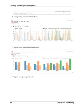
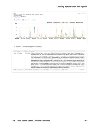

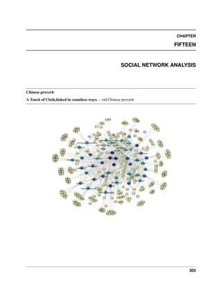
![Learning Apache Spark with Python
15.1 Introduction
15.2 Co-occurrence Network
Co-occurrence networks are generally used to provide a graphic visualization of potential relationships
between people, organizations, concepts or other entities represented within written material. The generation
and visualization of co-occurrence networks has become practical with the advent of electronically stored
text amenable to text mining.
15.2.1 Methodology
• Build Corpus C
• Build Document-Term matrix D based on Corpus C
• Compute Term-Document matrix 𝐷𝑇
• Adjacency Matrix 𝐴 = 𝐷𝑇 · 𝐷
There are four main components in this algorithm in the algorithm: Corpus C, Document-Term matrix D,
Term-Document matrix 𝐷𝑇 and Adjacency Matrix A. In this demo part, I will show how to build those four
main components.
Given that we have three groups of friends, they are
+-------------------------------------+
|words |
+-------------------------------------+
|[[george] [jimmy] [john] [peter]] |
|[[vincent] [george] [stefan] [james]]|
|[[emma] [james] [olivia] [george]] |
+-------------------------------------+
1. Corpus C
Then we can build the following corpus based on the unique elements in the given group data:
[u'george', u'james', u'jimmy', u'peter', u'stefan', u'vincent', u
˓
→'olivia', u'john', u'emma']
The corresponding elements frequency:
306 Chapter 15. Social Network Analysis](https://image.slidesharecdn.com/pyspark-230429134708-b35c8a19/85/pyspark-pdf-312-320.jpg)
![Learning Apache Spark with Python
2. Document-Term matrix D based on Corpus C (CountVectorizer)
from pyspark.ml.feature import CountVectorizer
count_vectorizer_wo = CountVectorizer(inputCol='term', outputCol=
˓
→'features')
# with total unique vocabulary
countVectorizer_mod_wo = count_vectorizer_wo.fit(df)
countVectorizer_twitter_wo = countVectorizer_mod_wo.transform(df)
# with truncated unique vocabulary (99%)
count_vectorizer = CountVectorizer(vocabSize=48,inputCol='term',
˓
→outputCol='features')
countVectorizer_mod = count_vectorizer.fit(df)
countVectorizer_twitter = countVectorizer_mod.transform(df)
+-------------------------------+
|features |
+-------------------------------+
|(9,[0,2,3,7],[1.0,1.0,1.0,1.0])|
|(9,[0,1,4,5],[1.0,1.0,1.0,1.0])|
|(9,[0,1,6,8],[1.0,1.0,1.0,1.0])|
+-------------------------------+
• Term-Document matrix 𝐷𝑇
RDD:
[array([ 1., 1., 1.]), array([ 0., 1., 1.]), array([ 1., 0., 0.
˓
→]),
array([ 1., 0., 0.]), array([ 0., 1., 0.]), array([ 0., 1., 0.
˓
→]),
array([ 0., 0., 1.]), array([ 1., 0., 0.]), array([ 0., 0., 1.
˓
→])]
15.2. Co-occurrence Network 307](https://image.slidesharecdn.com/pyspark-230429134708-b35c8a19/85/pyspark-pdf-313-320.jpg)
![Learning Apache Spark with Python
Matrix:
array([[ 1., 1., 1.],
[ 0., 1., 1.],
[ 1., 0., 0.],
[ 1., 0., 0.],
[ 0., 1., 0.],
[ 0., 1., 0.],
[ 0., 0., 1.],
[ 1., 0., 0.],
[ 0., 0., 1.]])
3. Adjacency Matrix 𝐴 = 𝐷𝑇 · 𝐷
RDD:
[array([ 1., 1., 1.]), array([ 0., 1., 1.]), array([ 1., 0., 0.
˓
→]),
array([ 1., 0., 0.]), array([ 0., 1., 0.]), array([ 0., 1., 0.
˓
→]),
array([ 0., 0., 1.]), array([ 1., 0., 0.]), array([ 0., 0., 1.
˓
→])]
Matrix:
array([[ 3., 2., 1., 1., 1., 1., 1., 1., 1.],
[ 2., 2., 0., 0., 1., 1., 1., 0., 1.],
[ 1., 0., 1., 1., 0., 0., 0., 1., 0.],
[ 1., 0., 1., 1., 0., 0., 0., 1., 0.],
[ 1., 1., 0., 0., 1., 1., 0., 0., 0.],
[ 1., 1., 0., 0., 1., 1., 0., 0., 0.],
[ 1., 1., 0., 0., 0., 0., 1., 0., 1.],
[ 1., 0., 1., 1., 0., 0., 0., 1., 0.],
[ 1., 1., 0., 0., 0., 0., 1., 0., 1.]])
15.2.2 Coding Puzzle from my interview
• Problem
The attached utf-8 encoded text file contains the tags associated with an online biomedical scientific article
formatted as follows (size: 100000). Each Scientific article is represented by a line in the file delimited by
carriage return.
+--------------------+
| words|
+--------------------+
|[ACTH Syndrome, E...|
|[Antibody Formati...|
|[Adaptation, Phys...|
|[Aerosol Propella...|
+--------------------+
only showing top 4 rows
308 Chapter 15. Social Network Analysis](https://image.slidesharecdn.com/pyspark-230429134708-b35c8a19/85/pyspark-pdf-314-320.jpg)
![Learning Apache Spark with Python
Write a program that, using this file as input, produces a list of pairs of tags which appear TOGETHER
in any order and position in at least fifty different Scientific articles. For example, in the above sample,
[Female] and [Humans] appear together twice, but every other pair appears only once. Your program should
output the pair list to stdout in the same form as the input (eg tag 1, tag 2n).
• My solution
The corresponding words frequency:
Fig. 1: Word frequency
Output:
+----------+------+-------+
| term.x|term.y| freq|
+----------+------+-------+
| Female|Humans|16741.0|
| Male|Humans|13883.0|
| Adult|Humans|10391.0|
| Male|Female| 9806.0|
|MiddleAged|Humans| 8181.0|
| Adult|Female| 7411.0|
| Adult| Male| 7240.0|
|MiddleAged| Male| 6328.0|
|MiddleAged|Female| 6002.0|
|MiddleAged| Adult| 5944.0|
+----------+------+-------+
only showing top 10 rows
The corresponding Co-occurrence network:
15.2. Co-occurrence Network 309](https://image.slidesharecdn.com/pyspark-230429134708-b35c8a19/85/pyspark-pdf-315-320.jpg)
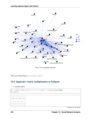
![Learning Apache Spark with Python
(continued from previous page)
|5.3|2.2|4.5|4.4|
|9.3|8.1|0.3|5.5|
|4.5|4.3|2.1|6.6|
+---+---+---+---+
2. main function for matrix multiplication in PySpark
from pyspark.sql import functions as F
from functools import reduce
# reference: https://stackoverflow.com/questions/44348527/matrix-
˓
→multiplication-at-a-in-pyspark
# do the sum of the multiplication that we want, and get
# one data frame for each column
colDFs = []
for c2 in df.columns:
colDFs.append( df.select( [ F.sum(df[c1]*df[c2]).alias("op_{0}".
˓
→format(i)) for i,c1 in enumerate(df.columns) ] ) )
# now union those separate data frames to build the "matrix"
mtxDF = reduce(lambda a,b: a.select(a.columns).union(b.select(a.columns)),
˓
→colDFs )
mtxDF.show()
+------------------+------------------+------------------+------------------+
| op_0| op_1| op_2| op_3|
+------------------+------------------+------------------+------------------+
| 152.45|118.88999999999999| 57.15|121.44000000000001|
|118.88999999999999|104.94999999999999| 38.93| 94.71|
| 57.15| 38.93|52.540000000000006| 55.99|
|121.44000000000001| 94.71| 55.99|110.10999999999999|
+------------------+------------------+------------------+------------------+
3. Validation with python version
import numpy as np
a = np.genfromtxt("matrix1.txt",delimiter=",")
np.dot(a.T, a)
array([[152.45, 118.89, 57.15, 121.44],
[118.89, 104.95, 38.93, 94.71],
[ 57.15, 38.93, 52.54, 55.99],
[121.44, 94.71, 55.99, 110.11]])
15.3. Appendix: matrix multiplication in PySpark 311](https://image.slidesharecdn.com/pyspark-230429134708-b35c8a19/85/pyspark-pdf-317-320.jpg)

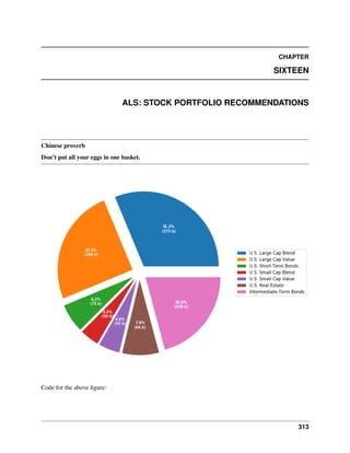
![Learning Apache Spark with Python
import numpy as np
import matplotlib.pyplot as plt
fig, ax = plt.subplots(figsize=(10, 8), subplot_kw=dict(aspect="equal"))
recipe = ["375 k U.S. Large Cap Blend",
"300 k U.S. Large Cap Value",
"75 k U.S. Short-Term Bonds",
"50 k U.S. Small Cap Blend",
"55 k U.S. Small Cap Value",
"95 k U.S. Real Estate",
"250 k Intermediate-Term Bonds"]
data = [float(x.split()[0]) for x in recipe]
ingredients = [' '.join(x.split()[2:]) for x in recipe]
print(data)
print(ingredients)
def func(pct, allvals):
absolute = int(pct/100.*np.sum(allvals))
return "{:.1f}%n({:d} k)".format(pct, absolute)
explode = np.empty(len(data))#(0.1, 0.1, 0.1, 0.1, 0.1, 0.1) # explode 1st
˓
→slice
explode.fill(0.1)
wedges, texts, autotexts = ax.pie(data, explode=explode, autopct=lambda pct:
˓
→func(pct, data),
textprops=dict(color="w"))
ax.legend(wedges, ingredients,
#title="Stock portfolio",
loc="center left",
bbox_to_anchor=(1, 0, 0.5, 1))
plt.setp(autotexts, size=8, weight="bold")
#ax.set_title("Stock portfolio")
plt.show()
16.1 Recommender systems
Recommender systems or recommendation systems (sometimes replacing “system” with a synonym such
as platform or engine) are a subclass of information filtering system that seek to predict the “rating” or
“preference” that a user would give to an item.”
The main idea is to build a matrix users R items rating values and try to factorize it, to recommend main
products rated by other users. A popular approach for this is matrix factorization is Alternating Least Squares
(ALS)
314 Chapter 16. ALS: Stock Portfolio Recommendations](https://image.slidesharecdn.com/pyspark-230429134708-b35c8a19/85/pyspark-pdf-320-320.jpg)
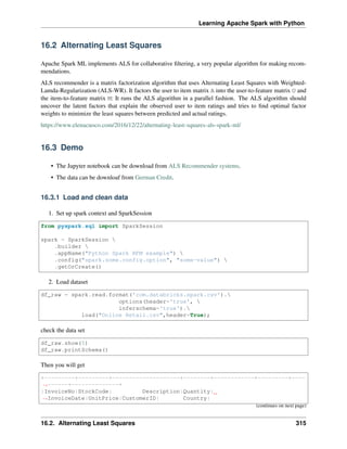
![Learning Apache Spark with Python
(continued from previous page)
+---------+---------+--------------------+--------+------------+---------+----
˓
→------+--------------+
| 536365| 85123A|WHITE HANGING HEA...| 6|12/1/10 8:26| 2.55|
˓
→ 17850|United Kingdom|
| 536365| 71053| WHITE METAL LANTERN| 6|12/1/10 8:26| 3.39|
˓
→ 17850|United Kingdom|
| 536365| 84406B|CREAM CUPID HEART...| 8|12/1/10 8:26| 2.75|
˓
→ 17850|United Kingdom|
| 536365| 84029G|KNITTED UNION FLA...| 6|12/1/10 8:26| 3.39|
˓
→ 17850|United Kingdom|
| 536365| 84029E|RED WOOLLY HOTTIE...| 6|12/1/10 8:26| 3.39|
˓
→ 17850|United Kingdom|
+---------+---------+--------------------+--------+------------+---------+----
˓
→------+--------------+
only showing top 5 rows
root
|-- InvoiceNo: string (nullable = true)
|-- StockCode: string (nullable = true)
|-- Description: string (nullable = true)
|-- Quantity: integer (nullable = true)
|-- InvoiceDate: string (nullable = true)
|-- UnitPrice: double (nullable = true)
|-- CustomerID: integer (nullable = true)
|-- Country: string (nullable = true)
3. Data clean and data manipulation
• check and remove the null values
from pyspark.sql.functions import count
def my_count(df_in):
df_in.agg( *[ count(c).alias(c) for c in df_in.columns ] ).show()
import pyspark.sql.functions as F
from pyspark.sql.functions import round
df_raw = df_raw.withColumn('Asset',round( F.col('Quantity') * F.col('UnitPrice
˓
→'), 2 ))
df = df_raw.withColumnRenamed('StockCode', 'Cusip')
.select('CustomerID','Cusip','Quantity','UnitPrice','Asset')
my_count(df)
+----------+------+--------+---------+------+
|CustomerID| Cusip|Quantity|UnitPrice| Asset|
+----------+------+--------+---------+------+
| 406829|541909| 541909| 541909|541909|
+----------+------+--------+---------+------+
Since the count results are not the same, we have some null value in the CustomerID column. We can
316 Chapter 16. ALS: Stock Portfolio Recommendations](https://image.slidesharecdn.com/pyspark-230429134708-b35c8a19/85/pyspark-pdf-322-320.jpg)
![Learning Apache Spark with Python
drop these records from the dataset.
df = df.filter(F.col('Asset')>=0)
df = df.dropna(how='any')
my_count(df)
+----------+------+--------+---------+------+
|CustomerID| Cusip|Quantity|UnitPrice| Asset|
+----------+------+--------+---------+------+
| 397924|397924| 397924| 397924|397924|
+----------+------+--------+---------+------+
df.show(3)
+----------+------+--------+---------+-----+
|CustomerID| Cusip|Quantity|UnitPrice|Asset|
+----------+------+--------+---------+-----+
| 17850|85123A| 6| 2.55| 15.3|
| 17850| 71053| 6| 3.39|20.34|
| 17850|84406B| 8| 2.75| 22.0|
+----------+------+--------+---------+-----+
only showing top 3 rows
• Convert the Cusip to consistent format
from pyspark.sql.functions import udf
from pyspark.sql.types import StringType, DoubleType
def toUpper(s):
return s.upper()
upper_udf = udf(lambda x: toUpper(x), StringType())
• Find the most top n stockes
pop = df.groupBy('Cusip')
.agg(F.count('CustomerID').alias('Customers'),F.round(F.sum('Asset'),2).
˓
→alias('TotalAsset'))
.sort([F.col('Customers'),F.col('TotalAsset')],ascending=[0,0])
pop.show(5)
+------+---------+----------+
| Cusip|Customers|TotalAsset|
+------+---------+----------+
|85123A| 2035| 100603.5|
| 22423| 1724| 142592.95|
|85099B| 1618| 85220.78|
| 84879| 1408| 56580.34|
| 47566| 1397| 68844.33|
+------+---------+----------+
only showing top 5 rows
16.3. Demo 317](https://image.slidesharecdn.com/pyspark-230429134708-b35c8a19/85/pyspark-pdf-323-320.jpg)
![Learning Apache Spark with Python
16.3.2 Build feature matrix
• Fetch the top n cusip list
top = 10
cusip_lst = pd.DataFrame(pop.select('Cusip').head(top)).astype('str').iloc[:,
˓
→0].tolist()
cusip_lst.insert(0,'CustomerID')
• Create the portfolio table for each customer
pivot_tab = df.groupBy('CustomerID').pivot('Cusip').sum('Asset')
pivot_tab = pivot_tab.fillna(0)
• Fetch the most n stock’s portfolio table for each customer
selected_tab = pivot_tab.select(cusip_lst)
selected_tab.show(4)
+----------+------+-----+------+-----+-----+-----+-----+-----+----+-----+
|CustomerID|85123A|22423|85099B|84879|47566|20725|22720|20727|POST|23203|
+----------+------+-----+------+-----+-----+-----+-----+-----+----+-----+
| 16503| 0.0| 0.0| 0.0| 0.0| 0.0| 0.0| 0.0| 33.0| 0.0| 0.0|
| 15727| 123.9| 25.5| 0.0| 0.0| 0.0| 33.0| 99.0| 0.0| 0.0| 0.0|
| 14570| 0.0| 0.0| 0.0| 0.0| 0.0| 0.0| 0.0| 0.0| 0.0| 0.0|
| 14450| 0.0| 0.0| 8.32| 0.0| 0.0| 0.0| 49.5| 0.0| 0.0| 0.0|
+----------+------+-----+------+-----+-----+-----+-----+-----+----+-----+
only showing top 4 rows
• Build the rating matrix
def elemwiseDiv(df_in):
num = len(df_in.columns)
temp = df_in.rdd.map(lambda x: list(flatten([x[0],[x[i]/float(sum(x[1:]))
if sum(x[1:])>0 else
˓
→x[i]
for i in range(1,
˓
→num)]])))
return spark.createDataFrame(temp,df_in.columns)
ratings = elemwiseDiv(selected_tab)
ratings.show(4)
+----------+------+-----+------+-----+-----+-----+-----+-----+----+-----+
|CustomerID|85123A|22423|85099B|84879|47566|20725|22720|20727|POST|23203|
+----------+------+-----+------+-----+-----+-----+-----+-----+----+-----+
| 16503| 0.0| 0.0| 0.0| 0.0| 0.0| 0.0| 0.0| 1.0| 0.0| 0.0|
| 15727| 0.44| 0.09| 0.0| 0.0| 0.0| 0.12| 0.35| 0.0| 0.0| 0.0|
(continues on next page)
318 Chapter 16. ALS: Stock Portfolio Recommendations](https://image.slidesharecdn.com/pyspark-230429134708-b35c8a19/85/pyspark-pdf-324-320.jpg)
![Learning Apache Spark with Python
(continued from previous page)
| 14570| 0.0| 0.0| 0.0| 0.0| 0.0| 0.0| 0.0| 0.0| 0.0| 0.0|
| 14450| 0.0| 0.0| 0.14| 0.0| 0.0| 0.0| 0.86| 0.0| 0.0| 0.0|
+----------+------+-----+------+-----+-----+-----+-----+-----+----+-----+
• Convert rating matrix to long table
from pyspark.sql.functions import array, col, explode, struct, lit
def to_long(df, by):
"""
reference: https://stackoverflow.com/questions/37864222/transpose-
˓
→column-to-row-with-spark
"""
# Filter dtypes and split into column names and type description
cols, dtypes = zip(*((c, t) for (c, t) in df.dtypes if c not in by))
# Spark SQL supports only homogeneous columns
assert len(set(dtypes)) == 1, "All columns have to be of the same type"
# Create and explode an array of (column_name, column_value) structs
kvs = explode(array([
struct(lit(c).alias("Cusip"), col(c).alias("rating")) for c in cols
])).alias("kvs")
df_all = to_long(ratings,['CustomerID'])
df_all.show(5)
+----------+------+------+
|CustomerID| Cusip|rating|
+----------+------+------+
| 16503|85123A| 0.0|
| 16503| 22423| 0.0|
| 16503|85099B| 0.0|
| 16503| 84879| 0.0|
| 16503| 47566| 0.0|
+----------+------+------+
only showing top 5 rows
• Convert the string Cusip to numerical index
from pyspark.ml.feature import StringIndexer
# Index labels, adding metadata to the label column
labelIndexer = StringIndexer(inputCol='Cusip',
outputCol='indexedCusip').fit(df_all)
df_all = labelIndexer.transform(df_all)
df_all.show(5, True)
df_all.printSchema()
+----------+------+------+------------+
(continues on next page)
16.3. Demo 319](https://image.slidesharecdn.com/pyspark-230429134708-b35c8a19/85/pyspark-pdf-325-320.jpg)
![Learning Apache Spark with Python
(continued from previous page)
|CustomerID| Cusip|rating|indexedCusip|
+----------+------+------+------------+
| 16503|85123A| 0.0| 6.0|
| 16503| 22423| 0.0| 9.0|
| 16503|85099B| 0.0| 5.0|
| 16503| 84879| 0.0| 1.0|
| 16503| 47566| 0.0| 0.0|
+----------+------+------+------------+
only showing top 5 rows
root
|-- CustomerID: long (nullable = true)
|-- Cusip: string (nullable = false)
|-- rating: double (nullable = true)
|-- indexedCusip: double (nullable = true)
16.3.3 Train model
• build train and test dataset
train, test = df_all.randomSplit([0.8,0.2])
train.show(5)
test.show(5)
+----------+-----+------------+-------------------+
|CustomerID|Cusip|indexedCusip| rating|
+----------+-----+------------+-------------------+
| 12940|20725| 2.0| 0.0|
| 12940|20727| 4.0| 0.0|
| 12940|22423| 9.0|0.49990198000392083|
| 12940|22720| 3.0| 0.0|
| 12940|23203| 7.0| 0.0|
+----------+-----+------------+-------------------+
only showing top 5 rows
+----------+-----+------------+------------------+
|CustomerID|Cusip|indexedCusip| rating|
+----------+-----+------------+------------------+
| 12940|84879| 1.0|0.1325230346990786|
| 13285|20725| 2.0|0.2054154995331466|
| 13285|20727| 4.0|0.2054154995331466|
| 13285|47566| 0.0| 0.0|
| 13623|23203| 7.0| 0.0|
+----------+-----+------------+------------------+
only showing top 5 rows
• train model
320 Chapter 16. ALS: Stock Portfolio Recommendations](https://image.slidesharecdn.com/pyspark-230429134708-b35c8a19/85/pyspark-pdf-326-320.jpg)
![Learning Apache Spark with Python
import itertools
from math import sqrt
from operator import add
import sys
from pyspark.ml.recommendation import ALS
from pyspark.ml.evaluation import RegressionEvaluator
evaluator = RegressionEvaluator(metricName="rmse", labelCol="rating",
predictionCol="prediction")
def computeRmse(model, data):
"""
Compute RMSE (Root mean Squared Error).
"""
predictions = model.transform(data)
rmse = evaluator.evaluate(predictions)
print("Root-mean-square error = " + str(rmse))
return rmse
#train models and evaluate them on the validation set
ranks = [4,5]
lambdas = [0.05]
numIters = [30]
bestModel = None
bestValidationRmse = float("inf")
bestRank = 0
bestLambda = -1.0
bestNumIter = -1
val = test.na.drop()
for rank, lmbda, numIter in itertools.product(ranks, lambdas, numIters):
als = ALS(rank=rank, maxIter=numIter, regParam=lmbda, numUserBlocks=10,
˓
→numItemBlocks=10, implicitPrefs=False,
alpha=1.0,
userCol="CustomerID", itemCol="indexedCusip", seed=1, ratingCol=
˓
→"rating", nonnegative=True)
model=als.fit(train)
validationRmse = computeRmse(model, val)
print("RMSE (validation) = %f for the model trained with " %
˓
→validationRmse +
"rank = %d, lambda = %.1f, and numIter = %d." % (rank, lmbda,
˓
→numIter))
if (validationRmse, bestValidationRmse):
bestModel = model
bestValidationRmse = validationRmse
bestRank = rank
bestLambda = lmbda
bestNumIter = numIter
model = bestModel
16.3. Demo 321](https://image.slidesharecdn.com/pyspark-230429134708-b35c8a19/85/pyspark-pdf-327-320.jpg)
![Learning Apache Spark with Python
16.3.4 Make prediction
• make prediction
topredict=test[test['rating']==0]
predictions=model.transform(topredict)
predictions.filter(predictions.prediction>0)
.sort([F.col('CustomerID'),F.col('Cusip')],ascending=[0,0]).show(5)
+----------+------+------------+------+------------+
|CustomerID| Cusip|indexedCusip|rating| prediction|
+----------+------+------------+------+------------+
| 18283| 47566| 0.0| 0.0| 0.01625076|
| 18282|85123A| 6.0| 0.0| 0.057172246|
| 18282| 84879| 1.0| 0.0| 0.059531752|
| 18282| 23203| 7.0| 0.0| 0.010502596|
| 18282| 22720| 3.0| 0.0| 0.053893942|
+----------+------+------------+------+------------+
only showing top 5 rows
322 Chapter 16. ALS: Stock Portfolio Recommendations](https://image.slidesharecdn.com/pyspark-230429134708-b35c8a19/85/pyspark-pdf-328-320.jpg)
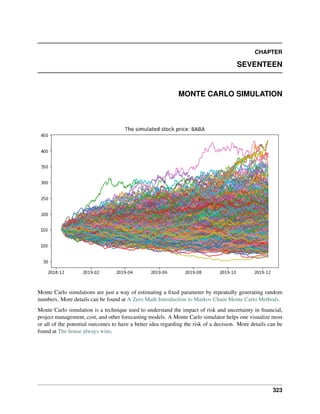
![Learning Apache Spark with Python
17.1 Simulating Casino Win
We assume that the player John has the 49% chance to win the game and the wager will be $5 per game.
import numpy as np
import pandas as pd
import matplotlib.pyplot as plt
start_m =100
wager = 5
bets = 100
trials = 1000
trans = np.vectorize(lambda t: -wager if t <=0.51 else wager)
fig = plt.figure(figsize=(10, 6))
ax = fig.add_subplot(1,1,1)
end_m = []
for i in range(trials):
money = reduce(lambda c, x: c + [c[-1] + x], trans(np.random.
˓
→random(bets)), [start_m])
end_m.append(money[-1])
plt.plot(money)
plt.ylabel('Player Money in $')
plt.xlabel('Number of bets')
plt.title(("John starts the game with $ %.2f and ends with $ %.2f")%(start_m,
˓
→sum(end_m)/len(end_m)))
plt.show()
324 Chapter 17. Monte Carlo Simulation](https://image.slidesharecdn.com/pyspark-230429134708-b35c8a19/85/pyspark-pdf-330-320.jpg)
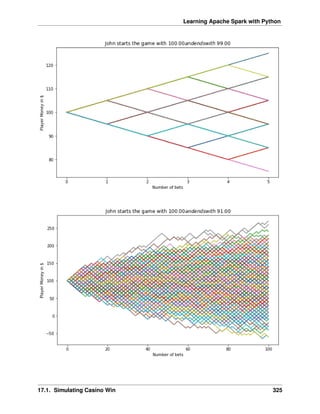
![Learning Apache Spark with Python
17.2 Simulating a Random Walk
17.2.1 Fetch the histrical stock price
1. Fecth the data. If you need the code for this piece, you can contact with me.
stock.tail(4)
+----------+----------+----------+----------+----------+----------+--------+
| Date| Open| High| Low| Close| Adj Close| Volume|
+----------+----------+----------+----------+----------+----------+--------+
|2018-12-07|155.399994|158.050003|151.729996|153.059998|153.059998|17447900|
|2018-12-10|150.389999|152.809998|147.479996|151.429993|151.429993|15525500|
|2018-12-11|155.259995|156.240005|150.899994|151.830002|151.830002|13651900|
|2018-12-12|155.240005|156.169998|151.429993| 151.5| 151.5|16597900|
+----------+----------+----------+----------+----------+----------+--------+
2. Convert the str type date to date type
stock['Date'] = pd.to_datetime(stock['Date'])
3. Data visualization
# Plot everything by leveraging the very powerful matplotlib package
width = 10
height = 6
data = stock
fig = plt.figure(figsize=(width, height))
ax = fig.add_subplot(1,1,1)
ax.plot(data.Date, data.Close, label='Close')
ax.plot(data.Date, data.High, label='High')
# ax.plot(data.Date, data.Low, label='Low')
ax.set_xlabel('Date')
ax.set_ylabel('price ($)')
ax.legend()
ax.set_title('Stock price: ' + ticker, y=1.01)
#plt.xticks(rotation=70)
plt.show()
# Plot everything by leveraging the very powerful matplotlib package
fig = plt.figure(figsize=(width, height))
ax = fig.add_subplot(1,1,1)
ax.plot(data.Date, data.Volume, label='Volume')
#ax.plot(data.Date, data.High, label='High')
# ax.plot(data.Date, data.Low, label='Low')
ax.set_xlabel('Date')
ax.set_ylabel('Volume')
ax.legend()
ax.set_title('Stock volume: ' + ticker, y=1.01)
#plt.xticks(rotation=70)
plt.show()
326 Chapter 17. Monte Carlo Simulation](https://image.slidesharecdn.com/pyspark-230429134708-b35c8a19/85/pyspark-pdf-332-320.jpg)
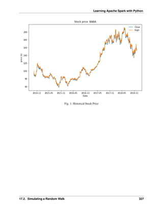
![Learning Apache Spark with Python
Fig. 2: Historical Stock Volume
17.2.2 Calulate the Compound Annual Growth Rate
The formula for Compound Annual Growth Rate (CAGR) is very useful for investment analysis. It may also
be referred to as the annualized rate of return or annual percent yield or effective annual rate, depending on
the algebraic form of the equation. Many investments such as stocks have returns that can vary wildly. The
CAGR formula allows you to calculate a “smoothed” rate of return that you can use to compare to other
investments. The formula is defined as (more details can be found at CAGR Calculator and Formula)
CAGR =
(︂
End Value
Start Value
)︂ 365
Days
− 1
days = (stock.Date.iloc[-1] - stock.Date.iloc[0]).days
cagr = ((((stock['Adj Close'].iloc[-1]) / stock['Adj Close'].iloc[0])) **
˓
→(365.0/days)) - 1
print ('CAGR =',str(round(cagr,4)*100)+"%")
mu = cagr
328 Chapter 17. Monte Carlo Simulation](https://image.slidesharecdn.com/pyspark-230429134708-b35c8a19/85/pyspark-pdf-334-320.jpg)
![Learning Apache Spark with Python
17.2.3 Calulate the annual volatility
A stock’s volatility is the variation in its price over a period of time. For example, one stock may have a
tendency to swing wildly higher and lower, while another stock may move in much steadier, less turbulent
way. Both stocks may end up at the same price at the end of day, but their path to that point can vary wildly.
First, we create a series of percentage returns and calculate the annual volatility of returns Annualizing
volatility. To present this volatility in annualized terms, we simply need to multiply our daily standard
deviation by the square root of 252. This assumes there are 252 trading days in a given year. More details
can be found at How to Calculate Annualized Volatility.
stock['Returns'] = stock['Adj Close'].pct_change()
vol = stock['Returns'].std()*np.sqrt(252)
17.2.4 Create matrix of daily returns
1. Create matrix of daily returns using random normal distribution Generates an RDD matrix comprised
of i.i.d. samples from the uniform distribution U(0.0, 1.0).
S = stock['Adj Close'].iloc[-1] #starting stock price (i.e. last available
˓
→real stock price)
T = 5 #Number of trading days
mu = cagr #Return
vol = vol #Volatility
trials = 10000
mat = RandomRDDs.normalVectorRDD(sc, trials, T, seed=1)
2. Transform the distribution in the generated RDD from U(0.0, 1.0) to U(a, b), use Random-
RDDs.uniformRDD(sc, n, p, seed) .map(lambda v: a + (b - a) * v)
a = mu/T
b = vol/math.sqrt(T)
v = mat.map(lambda x: a + (b - a)* x)
3. Convert Rdd matrix to dataframe
df = v.map(lambda x: [round(i,6)+1 for i in x]).toDF()
df.show(5)
+--------+--------+--------+--------+--------+
| _1| _2| _3| _4| _5|
+--------+--------+--------+--------+--------+
|0.935234|1.162894| 1.07972|1.238257|1.066136|
|0.878456|1.045922|0.990071|1.045552|0.854516|
|1.186472|0.944777|0.742247|0.940023|1.220934|
|0.872928|1.030882|1.248644|1.114262|1.063762|
| 1.09742|1.188537|1.137283|1.162548|1.024612|
+--------+--------+--------+--------+--------+
only showing top 5 rows
17.2. Simulating a Random Walk 329](https://image.slidesharecdn.com/pyspark-230429134708-b35c8a19/85/pyspark-pdf-335-320.jpg)
![Learning Apache Spark with Python
from pyspark.sql.functions import lit
S = stock['Adj Close'].iloc[-1]
price = df.withColumn('init_price' ,lit(S))
price.show(5)
+--------+--------+--------+--------+--------+----------+
| _1| _2| _3| _4| _5|init_price|
+--------+--------+--------+--------+--------+----------+
|0.935234|1.162894| 1.07972|1.238257|1.066136| 151.5|
|0.878456|1.045922|0.990071|1.045552|0.854516| 151.5|
|1.186472|0.944777|0.742247|0.940023|1.220934| 151.5|
|0.872928|1.030882|1.248644|1.114262|1.063762| 151.5|
| 1.09742|1.188537|1.137283|1.162548|1.024612| 151.5|
+--------+--------+--------+--------+--------+----------+
only showing top 5 rows
price = price.withColumn('day_0', col('init_price'))
price.show(5)
+--------+--------+--------+--------+--------+----------+-----+
| _1| _2| _3| _4| _5|init_price|day_0|
+--------+--------+--------+--------+--------+----------+-----+
|0.935234|1.162894| 1.07972|1.238257|1.066136| 151.5|151.5|
|0.878456|1.045922|0.990071|1.045552|0.854516| 151.5|151.5|
|1.186472|0.944777|0.742247|0.940023|1.220934| 151.5|151.5|
|0.872928|1.030882|1.248644|1.114262|1.063762| 151.5|151.5|
| 1.09742|1.188537|1.137283|1.162548|1.024612| 151.5|151.5|
+--------+--------+--------+--------+--------+----------+-----+
only showing top 5 rows
17.2.5 Monte Carlo Simulation
from pyspark.sql.functions import round
for name in price.columns[:-2]:
price = price.withColumn('day'+name, round(col(name)*col('init_price'),2))
price = price.withColumn('init_price',col('day'+name))
price.show(5)
+--------+--------+--------+--------+--------+----------+-----+------+------+-
˓
→-----+------+------+
| _1| _2| _3| _4| _5|init_price|day_0| day_1| day_2|
˓
→day_3| day_4| day_5|
+--------+--------+--------+--------+--------+----------+-----+------+------+-
˓
→-----+------+------+
|0.935234|1.162894| 1.07972|1.238257|1.066136| 234.87|151.5|141.69|164.
˓
→77|177.91| 220.3|234.87|
|0.878456|1.045922|0.990071|1.045552|0.854516| 123.14|151.5|133.09| 139.
˓
→2|137.82| 144.1|123.14| (continues on next page)
330 Chapter 17. Monte Carlo Simulation](https://image.slidesharecdn.com/pyspark-230429134708-b35c8a19/85/pyspark-pdf-336-320.jpg)
![Learning Apache Spark with Python
(continued from previous page)
|1.186472|0.944777|0.742247|0.940023|1.220934| 144.67|151.5|179.75|169.
˓
→82|126.05|118.49|144.67|
|0.872928|1.030882|1.248644|1.114262|1.063762| 201.77|151.5|132.25|136.
˓
→33|170.23|189.68|201.77|
| 1.09742|1.188537|1.137283|1.162548|1.024612| 267.7|151.5|166.26|197.
˓
→61|224.74|261.27| 267.7|
+--------+--------+--------+--------+--------+----------+-----+------+------+-
˓
→-----+------+------+
only showing top 5 rows
17.2.6 Summary
selected_col = [name for name in price.columns if 'day_' in name]
simulated = price.select(selected_col)
simulated.describe().show()
+-------+----------+------------------+------------------+------------------+-
˓
→-----------------+------------------+
|summary|2018-12-12| 2018-12-13| 2018-12-14| 2018-12-17|
˓
→ 2018-12-18| 2018-12-19|
+-------+----------+------------------+------------------+------------------+-
˓
→-----------------+------------------+
| count| 10000.0| 10000.0| 10000.0| 10000.0|
˓
→ 10000.0| 10000.0|
| mean| 151.5|155.11643700000002| 158.489058|162.23713200000003|
˓
→ 166.049375| 170.006525|
| std| 0.0|18.313783237787845|26.460919262517276| 33.
˓
→37780495150803|39.369101074463416|45.148120695490846|
| min| 151.5| 88.2| 74.54| 65.87|
˓
→ 68.21| 58.25|
| 25%| 151.5| 142.485| 140.15| 138.72|
˓
→ 138.365| 137.33|
| 50%| 151.5| 154.97| 157.175| 159.82|
˓
→ 162.59|165.04500000000002|
| 75%| 151.5| 167.445|175.48499999999999| 182.8625|
˓
→ 189.725| 196.975|
| max| 151.5| 227.48| 275.94| 319.17|
˓
→ 353.59| 403.68|
+-------+----------+------------------+------------------+------------------+-
˓
→-----------------+------------------+
data_plt = simulated.toPandas()
days = pd.date_range(stock['Date'].iloc[-1], periods= T+1,freq='B').date
width = 10
height = 6
fig = plt.figure(figsize=(width, height))
ax = fig.add_subplot(1,1,1)
(continues on next page)
17.2. Simulating a Random Walk 331](https://image.slidesharecdn.com/pyspark-230429134708-b35c8a19/85/pyspark-pdf-337-320.jpg)
![Learning Apache Spark with Python
(continued from previous page)
days = pd.date_range(stock['Date'].iloc[-1], periods= T+1,freq='B').date
for i in range(trials):
plt.plot(days, data_plt.iloc[i])
ax.set_xlabel('Date')
ax.set_ylabel('price ($)')
ax.set_title('Simulated Stock price: ' + ticker, y=1.01)
plt.show()
332 Chapter 17. Monte Carlo Simulation](https://image.slidesharecdn.com/pyspark-230429134708-b35c8a19/85/pyspark-pdf-338-320.jpg)
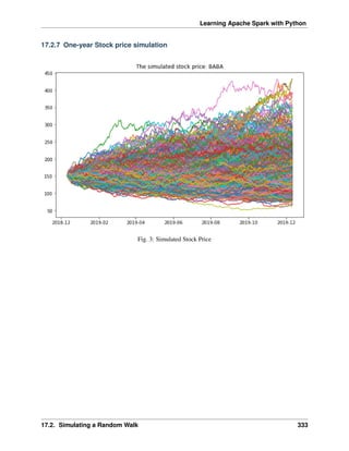
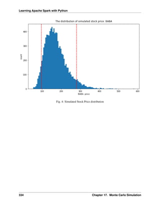
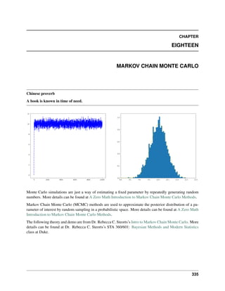
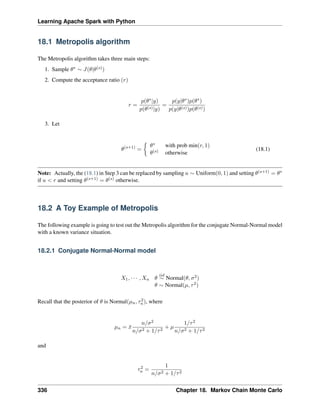
![Learning Apache Spark with Python
18.2.2 Example setup
The rest of the parameters are 𝜎2 = 1, 𝜏2 = 10, 𝜇 = 5, 𝑛 = 5 and
𝑦 = [9.37, 10.18, 9.16, 11.60, 10.33]
For this setup, we get that 𝜇𝑛 = 10.02745 and 𝜏2
𝑛 = 0.1960784.
18.2.3 Essential mathematical derivation
In the Metropolis algorithm, we need to compute the acceptance ratio 𝑟, i.e.
𝑟 =
𝑝(𝜃*|𝑥)
𝑝(𝜃(𝑠)|𝑥)
=
𝑝(𝑥|𝜃*)𝑝(𝜃*)
𝑝(𝑥|𝜃(𝑠))𝑝(𝜃(𝑠))
=
(︂ ∏︀
𝑖 dnorm(𝑥𝑖, 𝜃*, 𝜎)
∏︀
𝑖 dnorm(𝑥𝑖, 𝜃(𝑠), 𝜎)
)︂ (︂
dnorm(𝜃*, 𝜇, 𝜏)
dnorm(𝜃(𝑠), 𝜇, 𝜏)
)︂
In many cases, computing the ratio 𝑟 directly can be numerically unstable, however, this can be modified by
taking 𝑙𝑜𝑔𝑟. i.e.
𝑙𝑜𝑔𝑟 =
∑︁
𝑖
(︁
𝑙𝑜𝑔[dnorm(𝑥𝑖, 𝜃*
, 𝜎)] − 𝑙𝑜𝑔[dnorm(𝑥𝑖, 𝜃(𝑠)
, 𝜎)]
)︁
+
∑︁
𝑖
(︁
𝑙𝑜𝑔[dnorm(𝜃*
, 𝜇, 𝜏)] − 𝑙𝑜𝑔[dnorm(𝜃(𝑠)
, 𝜇, 𝜏)]
)︁
Then the criteria of the acceptance becomes: if 𝑙𝑜𝑔𝑢 < 𝑙𝑜𝑔𝑟, where 𝑢 is sample form the Uniform(0, 1).
18.3 Demos
Now, We generate 𝑆 iterations of the Metropolis algorithm starting at 𝜃(0) = 0 and using a normal proposal
distribution, where
𝜃(𝑠+1)
∼ Normal(𝜃(𝑠)
, 2).
18.3. Demos 337](https://image.slidesharecdn.com/pyspark-230429134708-b35c8a19/85/pyspark-pdf-343-320.jpg)
![Learning Apache Spark with Python
18.3.1 R results
# setting values
set.seed(1)
s2<-1
t2<-10
mu<-5; n<-5
# rounding the rnorm to 2 decimal places
y<-round(rnorm(n,10,1),2)
# mean of the normal posterior
mu.n<-( mean(y)*n/s2 + mu/t2 )/( n/s2+1/t2)
# variance of the normal posterior
t2.n<-1/(n/s2+1/t2)
# defining the data
y<-c(9.37, 10.18, 9.16, 11.60, 10.33)
####metropolis part####
##S = total num of simulations
theta<-0 ; delta<-2 ; S<-10000 ; THETA<-NULL ; set.seed(1)
for(s in 1:S){
## simulating our proposal
#the new value of theta
#print(theta)
theta.star<-rnorm(1,theta,sqrt(delta))
##taking the log of the ratio r
log.r<-( sum(dnorm(y,theta.star,sqrt(s2),log=TRUE))+
dnorm(theta.star,mu,sqrt(t2),log=TRUE))-
( sum(dnorm(y,theta,sqrt(s2),log=TRUE))+
dnorm(theta,mu,sqrt(t2),log=TRUE))
#print(log.r)
if(log(runif(1))<log.r) { theta<-theta.star }
##updating THETA
#print(log(runif(1)))
THETA<-c(THETA,theta)
}
##two plots: trace of theta and comparing the empirical distribution
##of simulated values to the true posterior
par(mar=c(3,3,1,1),mgp=c(1.75,.75,0))
par(mfrow=c(1,2))
# creating a sequence
skeep<-seq(10,S,by=10)
# making a trace place
plot(skeep,THETA[skeep],type="l",
xlab="iteration",ylab=expression(theta))
# making a histogram
hist(THETA[-(1:50)],prob=TRUE,main="",
xlab=expression(theta),ylab="density")
th<-seq(min(THETA),max(THETA),length=100)
lines(th,dnorm(th,mu.n,sqrt(t2.n)) )
338 Chapter 18. Markov Chain Monte Carlo](https://image.slidesharecdn.com/pyspark-230429134708-b35c8a19/85/pyspark-pdf-344-320.jpg)
![Learning Apache Spark with Python
Fig. 1: Histogram for the Metropolis algorithm with r
Figure. Histogram for the Metropolis algorithm with r shows a trace plot for this run as well as a histogram
for the Metropolis algorithm compared with a draw from the true normal density.
18.3.2 Python results
# coding: utf-8
# In[1]:
import numpy as np
# In[2]:
from scipy.stats import norm
def rnorm(n,mean,sd):
"""
same functions as rnorm in r
r: rnorm(n, mean=0, sd=1)
py: rvs(loc=0, scale=1, size=1, random_state=None)
"""
return norm.rvs(loc=mean,scale=sd,size=n)
(continues on next page)
18.3. Demos 339](https://image.slidesharecdn.com/pyspark-230429134708-b35c8a19/85/pyspark-pdf-345-320.jpg)
![Learning Apache Spark with Python
(continued from previous page)
def dnorm(x,mean,sd, log=False):
"""
same functions as dnorm in r
dnorm(x, mean=0, sd=1, log=FALSE)
pdf(x, loc=0, scale=1)
"""
if log:
return np.log(norm.pdf(x=x,loc=mean,scale=sd))
else:
return norm.pdf(x=x,loc=mean,scale=sd)
def runif(n,min=0, max=1):
"""
r: runif(n, min = 0, max = 1)
py: random.uniform(low=0.0, high=1.0, size=None)
"""
return np.random.uniform(min,max,size=n)
# In[3]:
s2 = 1
t2 = 10
mu = 5
n = 5
# In[4]:
y = rnorm(n,10,1)
y
# In[5]:
# mean of the normal posterior
mu_n = (np.mean(y)*n/s2 + mu/float(t2))/(n/float(s2)+1/float(t2))
mu_n
# In[6]:
# variance of the normal posterior
# t2.n<-1/(n/s2+1/t2)
t2_n = 1.0/(n/float(s2)+1.0/t2)
t2_n
# In[7]:
(continues on next page)
340 Chapter 18. Markov Chain Monte Carlo](https://image.slidesharecdn.com/pyspark-230429134708-b35c8a19/85/pyspark-pdf-346-320.jpg)
![Learning Apache Spark with Python
(continued from previous page)
# defining the data
# y<-c(9.37, 10.18, 9.16, 11.60, 10.33)
y = [9.37, 10.18, 9.16, 11.60, 10.33]
# In[8]:
mu_n = (np.mean(y)*n/s2 + mu/float(t2))/(n/float(s2)+1/float(t2))
mu_n
# In[9]:
####metropolis part####
##S = total num of simulations
# theta<-0 ; delta<-2 ; S<-10000 ; THETA<-NULL ; set.seed(1)
theta = 0
delta = 2
S = 10000
theta_v = []
# In[ ]:
for s in range(S):
theta_star = norm.rvs(theta,np.sqrt(delta),1)
logr = (sum(dnorm(y,theta_star,np.sqrt(s2),log=True)) +
sum(dnorm(theta_star,mu,np.sqrt(t2),log=True)))-
(sum(dnorm(y,theta,np.sqrt(s2),log=True)) +
sum(dnorm([theta],mu,np.sqrt(t2),log=True)))
#print(logr)
if np.log(runif(1))<logr:
theta = theta_star
#print(theta)
theta_v.append(theta)
# In[ ]:
import matplotlib.mlab as mlab
import matplotlib.pyplot as plt
plt.figure(figsize=(20, 8))
plt.subplot(1, 2, 1)
plt.plot(theta_v,'b-.')
(continues on next page)
18.3. Demos 341](https://image.slidesharecdn.com/pyspark-230429134708-b35c8a19/85/pyspark-pdf-347-320.jpg)
![Learning Apache Spark with Python
(continued from previous page)
plt.subplot(1, 2, 2)
#bins = np.arange(0, S, 10)
plt.hist(theta_v, density=True,bins='auto')
x = np.linspace(min(theta_v),max(theta_v),100)
y = norm.pdf(x,mu_n,np.sqrt(t2_n))
plt.plot(x,y,'y-.')
plt.xlim(right=12) # adjust the right leaving left unchanged
plt.xlim(left=8) # adjust the left leaving right unchanged
plt.show()
# In[ ]:
Fig. 2: Histogram for the Metropolis algorithm with python
Figure. Histogram for the Metropolis algorithm with python shows a trace plot for this run as well as a
histogram for the Metropolis algorithm compared with a draw from the true normal density.
342 Chapter 18. Markov Chain Monte Carlo](https://image.slidesharecdn.com/pyspark-230429134708-b35c8a19/85/pyspark-pdf-348-320.jpg)
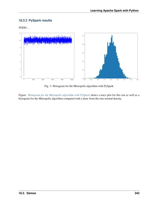

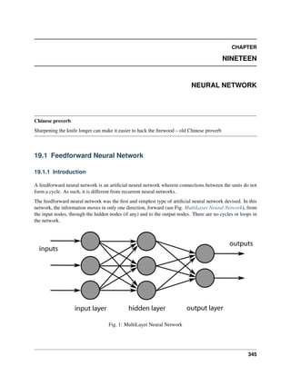
![Learning Apache Spark with Python
(continued from previous page)
string_to_float_udf = udf(string_to_float, DoubleType())
quality_udf = udf(lambda x: condition(x), StringType())
df= df.withColumn("quality", quality_udf("quality"))
4. Convert the data to dense vector
# convert the data to dense vector
def transData(data):
return data.rdd.map(lambda r: [r[-1], Vectors.dense(r[:-1])]).
toDF(['label','features'])
from pyspark.sql import Row
from pyspark.ml.linalg import Vectors
data= transData(df)
data.show()
5. Split the data into training and test sets (40% held out for testing)
# Split the data into train and test
(trainingData, testData) = data.randomSplit([0.6, 0.4])
6. Train neural network
# specify layers for the neural network:
# input layer of size 11 (features), two intermediate of size 5 and 4
# and output of size 7 (classes)
layers = [11, 5, 4, 4, 3 , 7]
# create the trainer and set its parameters
FNN = MultilayerPerceptronClassifier(labelCol="indexedLabel",
featuresCol="indexedFeatures",
maxIter=100, layers=layers,
blockSize=128, seed=1234)
# Convert indexed labels back to original labels.
labelConverter = IndexToString(inputCol="prediction", outputCol=
˓
→"predictedLabel",
labels=labelIndexer.labels)
# Chain indexers and forest in a Pipeline
from pyspark.ml import Pipeline
pipeline = Pipeline(stages=[labelIndexer, featureIndexer, FNN,
˓
→labelConverter])
# train the model
# Train model. This also runs the indexers.
model = pipeline.fit(trainingData)
7. Make predictions
# Make predictions.
predictions = model.transform(testData)
# Select example rows to display.
predictions.select("features","label","predictedLabel").show(5)
19.1. Feedforward Neural Network 347](https://image.slidesharecdn.com/pyspark-230429134708-b35c8a19/85/pyspark-pdf-353-320.jpg)
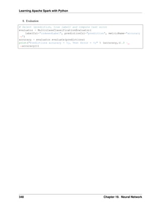
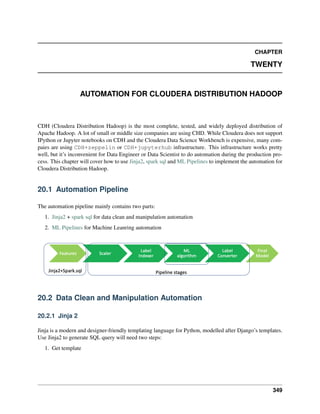
![Learning Apache Spark with Python
temp = """
SELECT project, timesheet, hours
FROM timesheet
WHERE user_id = {{ user_id }}
{% if project_id %}
AND project_id = {{ project_id }}
{% endif %}
"""
2. render the tempalte
args = {"user_id": u"runawayhorse",
"project_id": 123}
query= Template(temp).render(args)
print(query)
Then, you will get the following SQL query:
SELECT project, timesheet, hours
FROM timesheet
WHERE user_id = runawayhorse
AND project_id = 123
Note
The Jinja is smart then you think. If you try this
args = {"user_id": u"runawayhorse"}
query= Template(temp).render(args)
print(query)
Then, you will get the following SQL query:
SELECT project, timesheet, hours
FROM timesheet
WHERE user_id = runawayhorse
If you have a long query, you can use Iinja get_template to read the tempalte:
import os
from jinja2 import Template
from jinja2 import Environment, FileSystemLoader
path = os.path.abspath(os.path.join(sys.path[0]))
(continues on next page)
350 Chapter 20. Automation for Cloudera Distribution Hadoop](https://image.slidesharecdn.com/pyspark-230429134708-b35c8a19/85/pyspark-pdf-356-320.jpg)
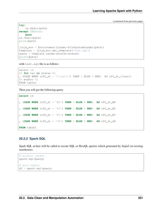
![Learning Apache Spark with Python
20.3 ML Pipeline Automation
I will not cover the details of the ML Pipeline at here, the interested reader is referred to ML Pipelines . The
The main steps for defining the stages are as follows:
scalering ='Standard'
from pyspark.ml.feature import Normalizer, StandardScaler, MinMaxScaler
if scalering=='Normal':
scaler = Normalizer(inputCol="features", outputCol="scaledFeatures", p=1.
˓
→0)
elif scalering=='Standard':
scaler = StandardScaler(inputCol="features", outputCol="scaledFeatures",
withStd=True, withMean=False)
else:
scaler = MinMaxScaler(inputCol="features", outputCol="scaledFeatures")
from pyspark.ml.feature import StringIndexer
# Index labels, adding metadata to the label column
labelIndexer = StringIndexer(inputCol='label',
outputCol='label').fit(transformed)
from pyspark.ml.feature import IndexToString
# Convert indexed labels back to original labels.
labelConverter = IndexToString(inputCol="prediction", outputCol=
˓
→"predictedLabel",
labels=labelIndexer.labels)
from pyspark.ml.classification import LogisticRegression
ml = LogisticRegression(featuresCol='scaledFeatures', labelCol='label',
˓
→maxIter=100, regParam=0.01, elasticNetParam=0.6)
# Chain indexers and tree in a Pipeline
pipeline_model = Pipeline(stages=[scaler,labelIndexer,ml,labelConverter])
# Train model. This also runs the indexers.
model = pipeline_model.fit(trainingData)
# Make predictions.
predictions = model.transform(testData)
352 Chapter 20. Automation for Cloudera Distribution Hadoop](https://image.slidesharecdn.com/pyspark-230429134708-b35c8a19/85/pyspark-pdf-358-320.jpg)
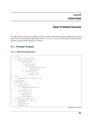
![Learning Apache Spark with Python
(continued from previous page)
| |-- top_level.txt
|-- README.md
|-- requirements.txt
|-- setup.py
|-- test
|-- spark-warehouse
|-- test1.py
|-- test2.py
From the above hierarchical structure, you will find that you have to have __init__.py in each directory.
I will explain the __init__.py file with the example below:
21.1.2 Set Up
from setuptools import setup, find_packages
try:
with open("README.md") as f:
long_description = f.read()
except IOError:
long_description = ""
try:
with open("requirements.txt") as f:
requirements = [x.strip() for x in f.read().splitlines() if x.strip()]
except IOError:
requirements = []
setup(name='PySParkTools',
install_requires=requirements,
version='1.0',
description='Python Spark Tools',
author='Wenqiang Feng',
author_email='von198@gmail.com',
url='https://github.com/runawayhorse001/PySparkTools',
packages=find_packages(),
long_description=long_description
)
21.1.3 ReadMe
# PySparkTools
This is my PySpark Tools. If you want to colne and install it, you can use
- clone
```{bash}
(continues on next page)
356 Chapter 21. Wrap PySpark Package](https://image.slidesharecdn.com/pyspark-230429134708-b35c8a19/85/pyspark-pdf-362-320.jpg)
. You can install
PySparkAudit using:
pip install PySparkAudit
358 Chapter 21. Wrap PySpark Package](https://image.slidesharecdn.com/pyspark-230429134708-b35c8a19/85/pyspark-pdf-364-320.jpg)
:
pip install PySparkAudit
22.2 Install from Repo
22.2.1 Clone the Repository
git clone https://github.com/runawayhorse001/PySparkAudit.git
22.2.2 Install
cd PySparkAudit
pip install -r requirements.txt
python setup.py install
22.3 Uninstall
pip uninstall PySparkAudit
359](https://image.slidesharecdn.com/pyspark-230429134708-b35c8a19/85/pyspark-pdf-365-320.jpg)
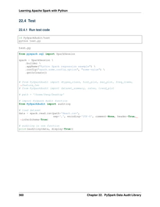

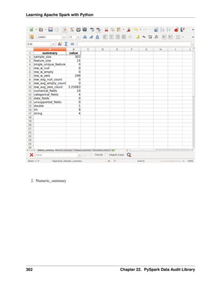
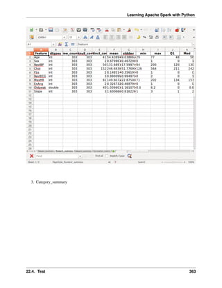
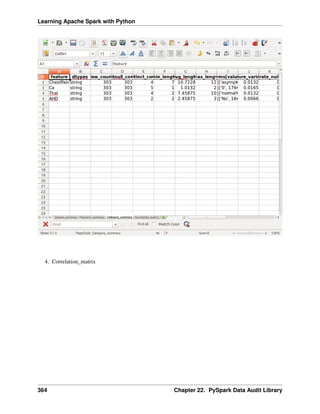
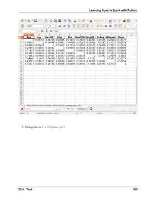
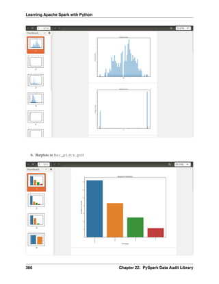
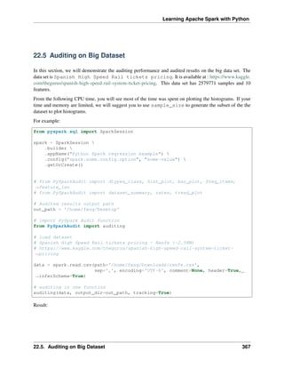
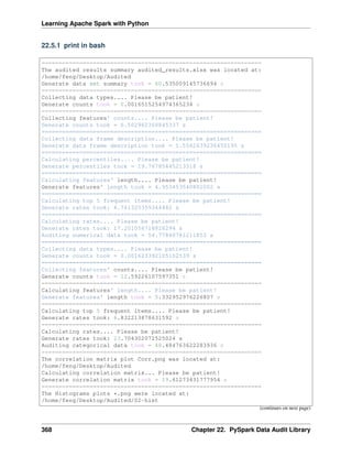
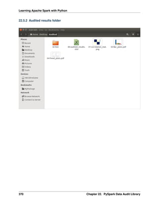
![CHAPTER
TWENTYTHREE
ZEPPELIN TO JUPYTER NOTEBOOK
The Zeppelin users may have same problem with me that the Zeppelin .json notebook is hard to open and
read. ze2nb: A piece of code to convert Zeppelin .json notebook to .ipynb Jupyter notebook, .py and
.html file. This library is based on Ryan Blue’s Jupyter/Zeppelin conversion: [jupyter-zeppelin]. The API
book can be found at ze2nb API or [zeppelin2nb]. You may download and distribute it. Please be aware,
however, that the note contains typos as well as inaccurate or incorrect description.
23.1 How to Install
23.1.1 Install with pip
You can install the ze2nb from [PyPI](https://pypi.org/project/ze2nb):
pip install ze2nb
23.1.2 Install from Repo
1. Clone the Repository
git clone https://github.com/runawayhorse001/ze2nb.git
2. Install
cd zeppelin2nb
pip install -r requirements.txt
python setup.py install
371](https://image.slidesharecdn.com/pyspark-230429134708-b35c8a19/85/pyspark-pdf-377-320.jpg)
![Learning Apache Spark with Python
23.1.3 Uninstall
pip uninstall ze2nb
23.2 Converting Demos
The following demos are designed to show how to use zepplin2nb to convert the .json to .ipynb ,
.py and .html.
23.2.1 Converting in one function
For example:
# import python library
import os, sys
# import zeppelin2nb module
from ze2nb import ze2nb
# scenario 1
# file and output at the current directory
# output path, the default output path will be the current directory
ze2nb('H2o_Sparking.json')
# scenario 2
output = os.path.abspath(os.path.join(sys.path[0])) +'/output'
ze2nb('H2o_Sparking.json', out_path=output, to_html=True, to_py=True)
# scenario 3
# with load and output path
load_path = '/Users/dt216661/Documents/MyJson/'
output = os.path.abspath(os.path.join(sys.path[0])) +'/output1'
ze2nb('H2o_GBM.json', load_path=load_path, out_path=output, to_html=True, to_
˓
→py=True)
23.2.2 Converted results
Result:
372 Chapter 23. Zeppelin to jupyter notebook](https://image.slidesharecdn.com/pyspark-230429134708-b35c8a19/85/pyspark-pdf-378-320.jpg)

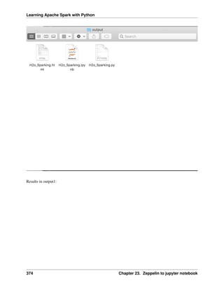

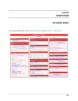
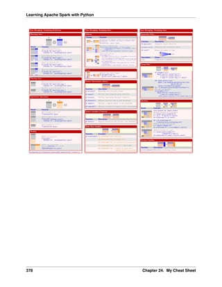
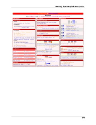

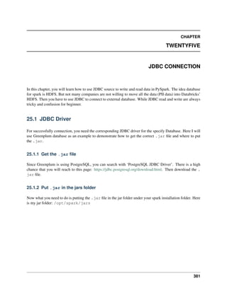
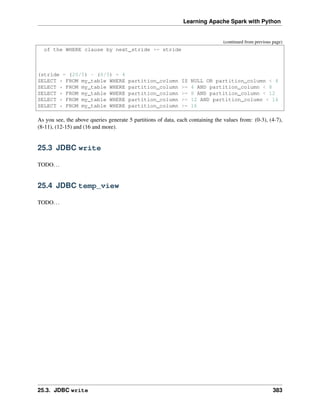

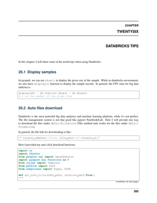
![Learning Apache Spark with Python
(continued from previous page)
Get file names and file path or relative path for the given HDFS
path. Note: os.listdir does not work in ``community.cloud.databricks``.
:param hdfs_path: the input HDFS path
:param relative_path: flag of return full path or the path relative to
``dbfs:/FileStore`` (We need the relative for the
file download.)
:return file_names: file names under the given path
:return relative_p: file paths, full path if ``relative_path=False``
else paths relative to ``bdfs:/FileStore``
"""
# get the file information
xx = dbutils.fs.ls(hdfs_path)
# get hdfs path and folder name
file_names = [list(xx[i])[1] for i in range(len(xx))]
hdfs_paths = [list(xx[i])[0] for i in range(len(xx))]
if relative_path:
try:
relative_p = [os.path.relpath(hdfs_path, 'dbfs:/FileStore') for hdfs_
˓
→path in hdfs_paths]
except:
print("Only suooprt the files under 'dbfs:/FileStore/'")
else:
relative_p = hdfs_paths
return file_names, relative_p
def azdb_files_download(files_path, cluster_address="https://community.cloud.
˓
→databricks.com",
cluster_no='4622560542654492'):
"""
List the files download links.
:param files_path: the given file path ot folder path
:param cluster_address: Your databricks cluster address, i.e. the link before
˓
→``/?o``
:param cluster_no: YOur databricks cluster number, i.e. the number after ``?
˓
→o=``
"""
if not os.path.isfile(files_path): # os.path.isdir(files_path):
file_names, files_path = get_hdfs_files(files_path)
if not isinstance(files_path, list):
files_path = [files_path]
urls = [f"{cluster_address}/files/{file_path}?o={cluster_no}" for file_path
˓
→in files_path]
(continues on next page)
386 Chapter 26. Databricks Tips](https://image.slidesharecdn.com/pyspark-230429134708-b35c8a19/85/pyspark-pdf-392-320.jpg)
![Learning Apache Spark with Python
(continued from previous page)
temp = """
<h2>AZDB files download</h2>
{% for i in range(len(urls)) %}
<a href="{{urls[i]}}" target='_blank'> Click me to download {
˓
→{files_path[i].split('/')[-1]}}</a> <br>
{% endfor %}
"""
html = Template(temp).render(files_path=files_path, urls=urls, len=len)
# get dbutils module
dbutils = IPython.get_ipython().user_ns["dbutils"]
dbutils.displayHTML(html)
Note: In commercial version of databricks, you can use
spark.conf.get("spark.databricks.clusterUsageTags.instanceWorkerEnvId")
to get the cluster_no. But it will not work for community version.
By using the above code, you can download the files relative to dbfs:/FileStore.
The files under dbfs:/FileStore/data
26.2. Auto files download 387](https://image.slidesharecdn.com/pyspark-230429134708-b35c8a19/85/pyspark-pdf-393-320.jpg)
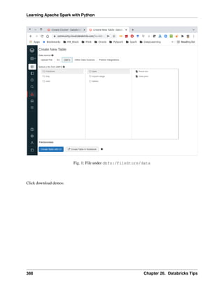
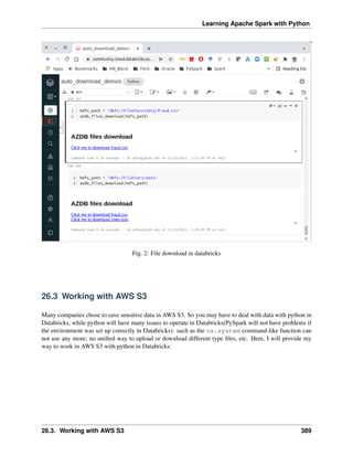
![Learning Apache Spark with Python
26.3.1 Credentials
I use Security Token Service (STS) to create the credentials to access AWS S3. STS enables you to re-
quest temporary, limited-privilege credentials for Identity and Access Management (IAM) users or for users
that you authenticate (federated users). More details can be found at: https://boto3.amazonaws.com/v1/
documentation/api/latest/reference/services/sts.html
import boto3
response = boto3.client('sts')
.assume_role(RoleArn='arn:aws:iam::123456789012:role/demo',
RoleSessionName='your_role_session_name')
credentials = response['Credentials']
26.3.2 File Upload to S3
The main idea at here is to save the file in memory or a temporary file, then use put_object to put the file
in S3. It’s a little bit tricky to save the corresponding formatted file in memory, I will list several common
types in the examples.
1. s3_file_upload Function
def s3_file_upload(data, path):
file_type = path.split('/')[-1].split('.')[-1].lower()
try:
content_type = s3_content_type(file_type)
except:
print('Do not support the current input type!!!')
s3_path = path.replace('s3://', '').replace('s3a://', '')
bucket = s3_path.split('/')[0]
key = s3_path.split('/', 1)[1]
try:
s3_resource.Bucket(bucket)
.put_object(Key=key,
Body=data,
ContentType=content_type,
ACL='public-read')
print(f"{key.split('/')[-1]} has been successfully saved in s3!")
except Exception as err:
print(err)
2. s3_content_type Function
def s3_content_type(file_type):
mapping = {png:image/png}
return mapping[file_type]
390 Chapter 26. Databricks Tips](https://image.slidesharecdn.com/pyspark-230429134708-b35c8a19/85/pyspark-pdf-396-320.jpg)
![Learning Apache Spark with Python
Note: The above method also works for .jpeg and .pdf format.
26.3.3 File Download from S3
The main idea is using the s3 resource function to download the file and save it at /temp as a temporary
file, the use the corresponding formatted functions to read it.
1. s3_file_download Function
def s3_file_download(path):
# extract bucket and key from the given path
s3_path = path.replace('s3://', '').replace('s3a://', '')
bucket = s3_path.split('/')[0]
key = s3_path.split('/', 1)[1]
# download file and save it as a temp file
file_name = os.path.join('/tmp', path.split('/')[-1])
s3_resource.Bucket(bucket).download_file(key, file_name)
# return saved file path
return file_name
2. Examples
>>> file_path = 'my_bucket/***/***/test/test.json'
>>> file_name = s3_file_download(file_path)
'/temp/test.json'
>>> joblib.load(filename)
26.3.4 File Management in S3
I mainly use my s3_fs to help me do the file management in S3.
1. s3_fs Function
The s3_fs is mainly based on s3fs package. The top-level class s3fs holds connection information
and allows typical file-system style operations like cp, mv, ls, walk, du, glob, etc. More details can be
found at: https://s3fs.readthedocs.io/en/latest/index.html
import s3fs
s3_fs = s3fs.S3FileSystem(anon=False,
key=credentials['AccessKeyId'],
secret=credentials['SecretAccessKey'],
token=credentials['SessionToken'])
2. Examples
402 Chapter 26. Databricks Tips](https://image.slidesharecdn.com/pyspark-230429134708-b35c8a19/85/pyspark-pdf-408-320.jpg)
![Learning Apache Spark with Python
Simple locate and read a file:
>>> s3_fs.ls('my-bucket')
['demo-file.csv']
>>> with fs.open('my-bucket/demo-file.csv', 'rb') as f:
... print(f.read())
b'UserIdtdatenuser_id1t2019-05-02nuser_id2t2019-12-02n'
26.4 delta format
TODO...
26.5 mlflow
TODO...
26.4. delta format 403](https://image.slidesharecdn.com/pyspark-230429134708-b35c8a19/85/pyspark-pdf-409-320.jpg)

![CHAPTER
TWENTYSEVEN
PYSPARK API
Those APIs are automatically generated from PySpark package, so all the CopyRights belong to Spark.
27.1 Stat API
class pyspark.ml.stat.ChiSquareTest
Note: Experimental
Conduct Pearson’s independence test for every feature against the label. For each feature, the (feature,
label) pairs are converted into a contingency matrix for which the Chi-squared statistic is computed.
All label and feature values must be categorical.
The null hypothesis is that the occurrence of the outcomes is statistically independent.
New in version 2.2.0.
static test(dataset, featuresCol, labelCol)
Perform a Pearson’s independence test using dataset.
Parameters
• dataset – DataFrame of categorical labels and categorical features. Real-
valued features will be treated as categorical for each distinct value.
• featuresCol – Name of features column in dataset, of type 𝑉 𝑒𝑐𝑡𝑜𝑟
(𝑉 𝑒𝑐𝑡𝑜𝑟𝑈𝐷𝑇).
• labelCol – Name of label column in dataset, of any numerical type.
Returns DataFrame containing the test result for every feature against the label. This
DataFrame will contain a single Row with the following fields: - 𝑝𝑉 𝑎𝑙𝑢𝑒𝑠 :
𝑉 𝑒𝑐𝑡𝑜𝑟 - 𝑑𝑒𝑔𝑟𝑒𝑒𝑠𝑂𝑓𝐹𝑟𝑒𝑒𝑑𝑜𝑚 : 𝐴𝑟𝑟𝑎𝑦[𝐼𝑛𝑡] - 𝑠𝑡𝑎𝑡𝑖𝑠𝑡𝑖𝑐𝑠 : 𝑉 𝑒𝑐𝑡𝑜𝑟 Each of these
fields has one value per feature.
405](https://image.slidesharecdn.com/pyspark-230429134708-b35c8a19/85/pyspark-pdf-411-320.jpg)
![Learning Apache Spark with Python
>>> from pyspark.ml.linalg import Vectors
>>> from pyspark.ml.stat import ChiSquareTest
>>> dataset = [[0, Vectors.dense([0, 0, 1])],
... [0, Vectors.dense([1, 0, 1])],
... [1, Vectors.dense([2, 1, 1])],
... [1, Vectors.dense([3, 1, 1])]]
>>> dataset = spark.createDataFrame(dataset, ["label", "features"])
>>> chiSqResult = ChiSquareTest.test(dataset, 'features', 'label')
>>> chiSqResult.select("degreesOfFreedom").collect()[0]
Row(degreesOfFreedom=[3, 1, 0])
New in version 2.2.0.
class pyspark.ml.stat.Correlation
Note: Experimental
Compute the correlation matrix for the input dataset of Vectors using the specified method. Methods
currently supported: 𝑝𝑒𝑎𝑟𝑠𝑜𝑛 (default), 𝑠𝑝𝑒𝑎𝑟𝑚𝑎𝑛.
Note: For Spearman, a rank correlation, we need to create an RDD[Double] for each column and sort
it in order to retrieve the ranks and then join the columns back into an RDD[Vector], which is fairly
costly. Cache the input Dataset before calling corr with 𝑚𝑒𝑡ℎ𝑜𝑑 =′ 𝑠𝑝𝑒𝑎𝑟𝑚𝑎𝑛′ to avoid recomputing
the common lineage.
New in version 2.2.0.
static corr(dataset, column, method='pearson')
Compute the correlation matrix with specified method using dataset.
Parameters
• dataset – A Dataset or a DataFrame.
• column – The name of the column of vectors for which the correlation coeffi-
cient needs to be computed. This must be a column of the dataset, and it must
contain Vector objects.
• method – String specifying the method to use for computing correlation. Sup-
ported: 𝑝𝑒𝑎𝑟𝑠𝑜𝑛 (default), 𝑠𝑝𝑒𝑎𝑟𝑚𝑎𝑛.
Returns A DataFrame that contains the correlation matrix of the column of vectors.
This DataFrame contains a single row and a single column of name ‘$METHOD-
NAME($COLUMN)’.
>>> from pyspark.ml.linalg import Vectors
>>> from pyspark.ml.stat import Correlation
>>> dataset = [[Vectors.dense([1, 0, 0, -2])],
... [Vectors.dense([4, 5, 0, 3])],
(continues on next page)
406 Chapter 27. PySpark API](https://image.slidesharecdn.com/pyspark-230429134708-b35c8a19/85/pyspark-pdf-412-320.jpg)
![Learning Apache Spark with Python
(continued from previous page)
... [Vectors.dense([6, 7, 0, 8])],
... [Vectors.dense([9, 0, 0, 1])]]
>>> dataset = spark.createDataFrame(dataset, ['features'])
>>> pearsonCorr = Correlation.corr(dataset, 'features', 'pearson').
˓
→collect()[0][0]
>>> print(str(pearsonCorr).replace('nan', 'NaN'))
DenseMatrix([[ 1. , 0.0556..., NaN, 0.4004...],
[ 0.0556..., 1. , NaN, 0.9135...],
[ NaN, NaN, 1. , NaN],
[ 0.4004..., 0.9135..., NaN, 1. ]])
>>> spearmanCorr = Correlation.corr(dataset, 'features', method=
˓
→'spearman').collect()[0][0]
>>> print(str(spearmanCorr).replace('nan', 'NaN'))
DenseMatrix([[ 1. , 0.1054..., NaN, 0.4 ],
[ 0.1054..., 1. , NaN, 0.9486... ],
[ NaN, NaN, 1. , NaN],
[ 0.4 , 0.9486... , NaN, 1. ]])
New in version 2.2.0.
class pyspark.ml.stat.KolmogorovSmirnovTest
Note: Experimental
Conduct the two-sided Kolmogorov Smirnov (KS) test for data sampled from a continuous distribu-
tion.
By comparing the largest difference between the empirical cumulative distribution of the sample data
and the theoretical distribution we can provide a test for the the null hypothesis that the sample data
comes from that theoretical distribution.
New in version 2.4.0.
static test(dataset, sampleCol, distName, *params)
Conduct a one-sample, two-sided Kolmogorov-Smirnov test for probability distribution equal-
ity. Currently supports the normal distribution, taking as parameters the mean and standard
deviation.
Parameters
• dataset – a Dataset or a DataFrame containing the sample of data to test.
• sampleCol – Name of sample column in dataset, of any numerical type.
• distName – a 𝑠𝑡𝑟𝑖𝑛𝑔 name for a theoretical distribution, currently only sup-
port “norm”.
• params – a list of 𝐷𝑜𝑢𝑏𝑙𝑒 values specifying the parameters to be used for the
theoretical distribution. For “norm” distribution, the parameters includes mean
and variance.
27.1. Stat API 407](https://image.slidesharecdn.com/pyspark-230429134708-b35c8a19/85/pyspark-pdf-413-320.jpg)
![Learning Apache Spark with Python
Returns A DataFrame that contains the Kolmogorov-Smirnov test result for the input
sampled data. This DataFrame will contain a single Row with the following fields:
- 𝑝𝑉 𝑎𝑙𝑢𝑒 : 𝐷𝑜𝑢𝑏𝑙𝑒 - 𝑠𝑡𝑎𝑡𝑖𝑠𝑡𝑖𝑐 : 𝐷𝑜𝑢𝑏𝑙𝑒
>>> from pyspark.ml.stat import KolmogorovSmirnovTest
>>> dataset = [[-1.0], [0.0], [1.0]]
>>> dataset = spark.createDataFrame(dataset, ['sample'])
>>> ksResult = KolmogorovSmirnovTest.test(dataset, 'sample', 'norm',
˓
→0.0, 1.0).first()
>>> round(ksResult.pValue, 3)
1.0
>>> round(ksResult.statistic, 3)
0.175
>>> dataset = [[2.0], [3.0], [4.0]]
>>> dataset = spark.createDataFrame(dataset, ['sample'])
>>> ksResult = KolmogorovSmirnovTest.test(dataset, 'sample', 'norm',
˓
→3.0, 1.0).first()
>>> round(ksResult.pValue, 3)
1.0
>>> round(ksResult.statistic, 3)
0.175
New in version 2.4.0.
class pyspark.ml.stat.Summarizer
Note: Experimental
Tools for vectorized statistics on MLlib Vectors. The methods in this package provide various statistics
for Vectors contained inside DataFrames. This class lets users pick the statistics they would like to
extract for a given column.
>>> from pyspark.ml.stat import Summarizer
>>> from pyspark.sql import Row
>>> from pyspark.ml.linalg import Vectors
>>> summarizer = Summarizer.metrics("mean", "count")
>>> df = sc.parallelize([Row(weight=1.0, features=Vectors.dense(1.0, 1.0,
˓
→ 1.0)),
... Row(weight=0.0, features=Vectors.dense(1.0, 2.0,
˓
→ 3.0))]).toDF()
>>> df.select(summarizer.summary(df.features, df.weight)).
˓
→show(truncate=False)
+-----------------------------------+
|aggregate_metrics(features, weight)|
+-----------------------------------+
|[[1.0,1.0,1.0], 1] |
+-----------------------------------+
>>> df.select(summarizer.summary(df.features)).show(truncate=False)
+--------------------------------+
(continues on next page)
408 Chapter 27. PySpark API](https://image.slidesharecdn.com/pyspark-230429134708-b35c8a19/85/pyspark-pdf-414-320.jpg)
![Learning Apache Spark with Python
(continued from previous page)
|aggregate_metrics(features, 1.0)|
+--------------------------------+
|[[1.0,1.5,2.0], 2] |
+--------------------------------+
>>> df.select(Summarizer.mean(df.features, df.weight)).
˓
→show(truncate=False)
+--------------+
|mean(features)|
+--------------+
|[1.0,1.0,1.0] |
+--------------+
>>> df.select(Summarizer.mean(df.features)).show(truncate=False)
+--------------+
|mean(features)|
+--------------+
|[1.0,1.5,2.0] |
+--------------+
New in version 2.4.0.
static count(col, weightCol=None)
return a column of count summary
New in version 2.4.0.
static max(col, weightCol=None)
return a column of max summary
New in version 2.4.0.
static mean(col, weightCol=None)
return a column of mean summary
New in version 2.4.0.
static metrics(*metrics)
Given a list of metrics, provides a builder that it turns computes metrics from a column.
See the documentation of [[Summarizer]] for an example.
The following metrics are accepted (case sensitive):
• mean: a vector that contains the coefficient-wise mean.
• variance: a vector tha contains the coefficient-wise variance.
• count: the count of all vectors seen.
• numNonzeros: a vector with the number of non-zeros for each coefficients
• max: the maximum for each coefficient.
• min: the minimum for each coefficient.
• normL2: the Euclidian norm for each coefficient.
27.1. Stat API 409](https://image.slidesharecdn.com/pyspark-230429134708-b35c8a19/85/pyspark-pdf-415-320.jpg)
![Learning Apache Spark with Python
Returns an aggregate column that contains the statistics. The exact content of this
structure is determined during the creation of the builder.
New in version 2.4.0.
27.2 Regression API
class pyspark.ml.regression.AFTSurvivalRegression(*args, **kwargs)
Note: Experimental
Accelerated Failure Time (AFT) Model Survival Regression
Fit a parametric AFT survival regression model based on the Weibull distribution of the survival time.
See also:
AFT Model
>>> from pyspark.ml.linalg import Vectors
>>> df = spark.createDataFrame([
... (1.0, Vectors.dense(1.0), 1.0),
... (1e-40, Vectors.sparse(1, [], []), 0.0)], ["label", "features",
˓
→"censor"])
>>> aftsr = AFTSurvivalRegression()
>>> model = aftsr.fit(df)
>>> model.predict(Vectors.dense(6.3))
1.0
>>> model.predictQuantiles(Vectors.dense(6.3))
DenseVector([0.0101, 0.0513, 0.1054, 0.2877, 0.6931, 1.3863, 2.3026, 2.
˓
→9957, 4.6052])
>>> model.transform(df).show()
+-------+---------+------+----------+
| label| features|censor|prediction|
+-------+---------+------+----------+
| 1.0| [1.0]| 1.0| 1.0|
|1.0E-40|(1,[],[])| 0.0| 1.0|
+-------+---------+------+----------+
...
>>> aftsr_path = temp_path + "/aftsr"
>>> aftsr.save(aftsr_path)
>>> aftsr2 = AFTSurvivalRegression.load(aftsr_path)
>>> aftsr2.getMaxIter()
100
>>> model_path = temp_path + "/aftsr_model"
>>> model.save(model_path)
>>> model2 = AFTSurvivalRegressionModel.load(model_path)
>>> model.coefficients == model2.coefficients
True
(continues on next page)
27.2. Regression API 411](https://image.slidesharecdn.com/pyspark-230429134708-b35c8a19/85/pyspark-pdf-417-320.jpg)
![Learning Apache Spark with Python
(continued from previous page)
>>> model.intercept == model2.intercept
True
>>> model.scale == model2.scale
True
New in version 1.6.0.
getCensorCol()
Gets the value of censorCol or its default value.
New in version 1.6.0.
getQuantileProbabilities()
Gets the value of quantileProbabilities or its default value.
New in version 1.6.0.
getQuantilesCol()
Gets the value of quantilesCol or its default value.
New in version 1.6.0.
setCensorCol(value)
Sets the value of censorCol.
New in version 1.6.0.
setParams(featuresCol='features', labelCol='label', predictionCol='prediction', fitInter-
cept=True, maxIter=100, tol=1e-06, censorCol='censor', quantileProbabili-
ties=[0.01, 0.05, 0.1, 0.25, 0.5, 0.75, 0.9, 0.95, 0.99], quantilesCol=None, ag-
gregationDepth=2)
setParams(self, featuresCol=”features”, labelCol=”label”, predictionCol=”prediction”, fitInter-
cept=True, maxIter=100, tol=1E-6, censorCol=”censor”, quantileProbabilities=[0.01, 0.05, 0.1,
0.25, 0.5, 0.75, 0.9, 0.95, 0.99], quantilesCol=None, aggregationDepth=2):
New in version 1.6.0.
setQuantileProbabilities(value)
Sets the value of quantileProbabilities.
New in version 1.6.0.
setQuantilesCol(value)
Sets the value of quantilesCol.
New in version 1.6.0.
class pyspark.ml.regression.AFTSurvivalRegressionModel(java_model=None)
Note: Experimental
Model fitted by AFTSurvivalRegression.
412 Chapter 27. PySpark API](https://image.slidesharecdn.com/pyspark-230429134708-b35c8a19/85/pyspark-pdf-418-320.jpg)
![Learning Apache Spark with Python
>>> from pyspark.ml.linalg import Vectors
>>> df = spark.createDataFrame([
... (1.0, Vectors.dense(1.0)),
... (0.0, Vectors.sparse(1, [], []))], ["label", "features"])
>>> dt = DecisionTreeRegressor(maxDepth=2, varianceCol="variance")
>>> model = dt.fit(df)
>>> model.depth
1
>>> model.numNodes
3
>>> model.featureImportances
SparseVector(1, {0: 1.0})
>>> model.numFeatures
1
>>> test0 = spark.createDataFrame([(Vectors.dense(-1.0),)], ["features"])
>>> model.transform(test0).head().prediction
0.0
>>> test1 = spark.createDataFrame([(Vectors.sparse(1, [0], [1.0]),)], [
˓
→"features"])
>>> model.transform(test1).head().prediction
1.0
>>> dtr_path = temp_path + "/dtr"
>>> dt.save(dtr_path)
>>> dt2 = DecisionTreeRegressor.load(dtr_path)
>>> dt2.getMaxDepth()
2
>>> model_path = temp_path + "/dtr_model"
>>> model.save(model_path)
>>> model2 = DecisionTreeRegressionModel.load(model_path)
>>> model.numNodes == model2.numNodes
True
>>> model.depth == model2.depth
True
>>> model.transform(test1).head().variance
0.0
New in version 1.4.0.
setParams(self, featuresCol='features', labelCol='label', predictionCol='prediction',
maxDepth=5, maxBins=32, minInstancesPerNode=1, minInfoGain=0.0,
maxMemoryInMB=256, cacheNodeIds=False, checkpointInterval=10, impu-
rity='variance', seed=None, varianceCol=None)
Sets params for the DecisionTreeRegressor.
New in version 1.4.0.
class pyspark.ml.regression.GBTRegressionModel(java_model=None)
Model fitted by GBTRegressor.
New in version 1.4.0.
evaluateEachIteration(dataset, loss)
Method to compute error or loss for every iteration of gradient boosting.
414 Chapter 27. PySpark API](https://image.slidesharecdn.com/pyspark-230429134708-b35c8a19/85/pyspark-pdf-420-320.jpg)
![Learning Apache Spark with Python
Parameters
• dataset – Test dataset to evaluate model on, where dataset is an instance of
pyspark.sql.DataFrame
• loss – The loss function used to compute error. Supported options: squared,
absolute
New in version 2.4.0.
property featureImportances
Estimate of the importance of each feature.
Each feature’s importance is the average of its importance across all trees in the ensemble The
importance vector is normalized to sum to 1. This method is suggested by Hastie et al. (Hastie,
Tibshirani, Friedman. “The Elements of Statistical Learning, 2nd Edition.” 2001.) and follows
the implementation from scikit-learn.
See also:
DecisionTreeRegressionModel.featureImportances
New in version 2.0.0.
property trees
These have null parent Estimators.
New in version 2.0.0.
Type Trees in this ensemble. Warning
class pyspark.ml.regression.GBTRegressor(*args, **kwargs)
Gradient-Boosted Trees (GBTs) learning algorithm for regression. It supports both continuous and
categorical features.
>>> from numpy import allclose
>>> from pyspark.ml.linalg import Vectors
>>> df = spark.createDataFrame([
... (1.0, Vectors.dense(1.0)),
... (0.0, Vectors.sparse(1, [], []))], ["label", "features"])
>>> gbt = GBTRegressor(maxIter=5, maxDepth=2, seed=42)
>>> print(gbt.getImpurity())
variance
>>> print(gbt.getFeatureSubsetStrategy())
all
>>> model = gbt.fit(df)
>>> model.featureImportances
SparseVector(1, {0: 1.0})
>>> model.numFeatures
1
>>> allclose(model.treeWeights, [1.0, 0.1, 0.1, 0.1, 0.1])
True
>>> test0 = spark.createDataFrame([(Vectors.dense(-1.0),)], ["features"])
>>> model.transform(test0).head().prediction
0.0
(continues on next page)
27.2. Regression API 415](https://image.slidesharecdn.com/pyspark-230429134708-b35c8a19/85/pyspark-pdf-421-320.jpg)
![Learning Apache Spark with Python
(continued from previous page)
>>> test1 = spark.createDataFrame([(Vectors.sparse(1, [0], [1.0]),)], [
˓
→"features"])
>>> model.transform(test1).head().prediction
1.0
>>> gbtr_path = temp_path + "gbtr"
>>> gbt.save(gbtr_path)
>>> gbt2 = GBTRegressor.load(gbtr_path)
>>> gbt2.getMaxDepth()
2
>>> model_path = temp_path + "gbtr_model"
>>> model.save(model_path)
>>> model2 = GBTRegressionModel.load(model_path)
>>> model.featureImportances == model2.featureImportances
True
>>> model.treeWeights == model2.treeWeights
True
>>> model.trees
[DecisionTreeRegressionModel (uid=...) of depth...,
˓
→DecisionTreeRegressionModel...]
>>> validation = spark.createDataFrame([(0.0, Vectors.dense(-1.0))],
... ["label", "features"])
>>> model.evaluateEachIteration(validation, "squared")
[0.0, 0.0, 0.0, 0.0, 0.0]
New in version 1.4.0.
getLossType()
Gets the value of lossType or its default value.
New in version 1.4.0.
setFeatureSubsetStrategy(value)
Sets the value of featureSubsetStrategy.
New in version 2.4.0.
setLossType(value)
Sets the value of lossType.
New in version 1.4.0.
setParams(self, featuresCol='features', labelCol='label', predictionCol='prediction',
maxDepth=5, maxBins=32, minInstancesPerNode=1, minInfoGain=0.0,
maxMemoryInMB=256, cacheNodeIds=False, subsamplingRate=1.0, check-
pointInterval=10, lossType='squared', maxIter=20, stepSize=0.1, seed=None,
impurity='variance', featureSubsetStrategy='all')
Sets params for Gradient Boosted Tree Regression.
New in version 1.4.0.
class pyspark.ml.regression.GeneralizedLinearRegression(*args,
**kwargs)
416 Chapter 27. PySpark API](https://image.slidesharecdn.com/pyspark-230429134708-b35c8a19/85/pyspark-pdf-422-320.jpg)
![Learning Apache Spark with Python
Note: Experimental
Generalized Linear Regression.
Fit a Generalized Linear Model specified by giving a symbolic description of the linear predictor
(link function) and a description of the error distribution (family). It supports “gaussian”, “binomial”,
“poisson”, “gamma” and “tweedie” as family. Valid link functions for each family is listed below.
The first link function of each family is the default one.
• “gaussian” -> “identity”, “log”, “inverse”
• “binomial” -> “logit”, “probit”, “cloglog”
• “poisson” -> “log”, “identity”, “sqrt”
• “gamma” -> “inverse”, “identity”, “log”
• “tweedie” -> power link function specified through “linkPower”. The default link power in the
tweedie family is 1 - variancePower.
See also:
GLM
>>> from pyspark.ml.linalg import Vectors
>>> df = spark.createDataFrame([
... (1.0, Vectors.dense(0.0, 0.0)),
... (1.0, Vectors.dense(1.0, 2.0)),
... (2.0, Vectors.dense(0.0, 0.0)),
... (2.0, Vectors.dense(1.0, 1.0)),], ["label", "features"])
>>> glr = GeneralizedLinearRegression(family="gaussian", link="identity",
˓
→ linkPredictionCol="p")
>>> model = glr.fit(df)
>>> transformed = model.transform(df)
>>> abs(transformed.head().prediction - 1.5) < 0.001
True
>>> abs(transformed.head().p - 1.5) < 0.001
True
>>> model.coefficients
DenseVector([1.5..., -1.0...])
>>> model.numFeatures
2
>>> abs(model.intercept - 1.5) < 0.001
True
>>> glr_path = temp_path + "/glr"
>>> glr.save(glr_path)
>>> glr2 = GeneralizedLinearRegression.load(glr_path)
>>> glr.getFamily() == glr2.getFamily()
True
>>> model_path = temp_path + "/glr_model"
>>> model.save(model_path)
>>> model2 = GeneralizedLinearRegressionModel.load(model_path)
>>> model.intercept == model2.intercept
(continues on next page)
27.2. Regression API 417](https://image.slidesharecdn.com/pyspark-230429134708-b35c8a19/85/pyspark-pdf-423-320.jpg)
![Learning Apache Spark with Python
(continued from previous page)
True
>>> model.coefficients[0] == model2.coefficients[0]
True
New in version 2.0.0.
getFamily()
Gets the value of family or its default value.
New in version 2.0.0.
getLink()
Gets the value of link or its default value.
New in version 2.0.0.
getLinkPower()
Gets the value of linkPower or its default value.
New in version 2.2.0.
getLinkPredictionCol()
Gets the value of linkPredictionCol or its default value.
New in version 2.0.0.
getOffsetCol()
Gets the value of offsetCol or its default value.
New in version 2.3.0.
getVariancePower()
Gets the value of variancePower or its default value.
New in version 2.2.0.
setFamily(value)
Sets the value of family.
New in version 2.0.0.
setLink(value)
Sets the value of link.
New in version 2.0.0.
setLinkPower(value)
Sets the value of linkPower.
New in version 2.2.0.
setLinkPredictionCol(value)
Sets the value of linkPredictionCol.
New in version 2.0.0.
418 Chapter 27. PySpark API](https://image.slidesharecdn.com/pyspark-230429134708-b35c8a19/85/pyspark-pdf-424-320.jpg)
![Learning Apache Spark with Python
If GeneralizedLinearRegression.fitIntercept is set to True, then the last ele-
ment returned corresponds to the intercept.
New in version 2.0.0.
class pyspark.ml.regression.IsotonicRegression(*args, **kwargs)
Currently implemented using parallelized pool adjacent violators algorithm. Only univariate (single
feature) algorithm supported.
>>> from pyspark.ml.linalg import Vectors
>>> df = spark.createDataFrame([
... (1.0, Vectors.dense(1.0)),
... (0.0, Vectors.sparse(1, [], []))], ["label", "features"])
>>> ir = IsotonicRegression()
>>> model = ir.fit(df)
>>> test0 = spark.createDataFrame([(Vectors.dense(-1.0),)], ["features"])
>>> model.transform(test0).head().prediction
0.0
>>> model.boundaries
DenseVector([0.0, 1.0])
>>> ir_path = temp_path + "/ir"
>>> ir.save(ir_path)
>>> ir2 = IsotonicRegression.load(ir_path)
>>> ir2.getIsotonic()
True
>>> model_path = temp_path + "/ir_model"
>>> model.save(model_path)
>>> model2 = IsotonicRegressionModel.load(model_path)
>>> model.boundaries == model2.boundaries
True
>>> model.predictions == model2.predictions
True
New in version 1.6.0.
getFeatureIndex()
Gets the value of featureIndex or its default value.
getIsotonic()
Gets the value of isotonic or its default value.
setFeatureIndex(value)
Sets the value of featureIndex.
setIsotonic(value)
Sets the value of isotonic.
setParams(featuresCol='features', labelCol='label', predictionCol='prediction', weight-
Col=None, isotonic=True, featureIndex=0)
setParams(self, featuresCol=”features”, labelCol=”label”, predictionCol=”prediction”, weight-
Col=None, isotonic=True, featureIndex=0): Set the params for IsotonicRegression.
class pyspark.ml.regression.IsotonicRegressionModel(java_model=None)
Model fitted by IsotonicRegression.
422 Chapter 27. PySpark API](https://image.slidesharecdn.com/pyspark-230429134708-b35c8a19/85/pyspark-pdf-428-320.jpg)
![Learning Apache Spark with Python
New in version 1.6.0.
property boundaries
Boundaries in increasing order for which predictions are known.
New in version 1.6.0.
property predictions
Predictions associated with the boundaries at the same index, monotone because of isotonic
regression.
New in version 1.6.0.
class pyspark.ml.regression.LinearRegression(*args, **kwargs)
Linear regression.
The learning objective is to minimize the specified loss function, with regularization. This supports
two kinds of loss:
• squaredError (a.k.a squared loss)
• huber (a hybrid of squared error for relatively small errors and absolute error for relatively large
ones, and we estimate the scale parameter from training data)
This supports multiple types of regularization:
• none (a.k.a. ordinary least squares)
• L2 (ridge regression)
• L1 (Lasso)
• L2 + L1 (elastic net)
Note: Fitting with huber loss only supports none and L2 regularization.
>>> from pyspark.ml.linalg import Vectors
>>> df = spark.createDataFrame([
... (1.0, 2.0, Vectors.dense(1.0)),
... (0.0, 2.0, Vectors.sparse(1, [], []))], ["label", "weight",
˓
→"features"])
>>> lr = LinearRegression(maxIter=5, regParam=0.0, solver="normal",
˓
→weightCol="weight")
>>> model = lr.fit(df)
>>> test0 = spark.createDataFrame([(Vectors.dense(-1.0),)], ["features"])
>>> abs(model.transform(test0).head().prediction - (-1.0)) < 0.001
True
>>> abs(model.coefficients[0] - 1.0) < 0.001
True
>>> abs(model.intercept - 0.0) < 0.001
True
>>> test1 = spark.createDataFrame([(Vectors.sparse(1, [0], [1.0]),)], [
˓
→"features"])
>>> abs(model.transform(test1).head().prediction - 1.0) < 0.001
True
>>> lr.setParams("vector")
(continues on next page)
27.2. Regression API 423](https://image.slidesharecdn.com/pyspark-230429134708-b35c8a19/85/pyspark-pdf-429-320.jpg)
![Learning Apache Spark with Python
(continued from previous page)
Traceback (most recent call last):
...
TypeError: Method setParams forces keyword arguments.
>>> lr_path = temp_path + "/lr"
>>> lr.save(lr_path)
>>> lr2 = LinearRegression.load(lr_path)
>>> lr2.getMaxIter()
5
>>> model_path = temp_path + "/lr_model"
>>> model.save(model_path)
>>> model2 = LinearRegressionModel.load(model_path)
>>> model.coefficients[0] == model2.coefficients[0]
True
>>> model.intercept == model2.intercept
True
>>> model.numFeatures
1
>>> model.write().format("pmml").save(model_path + "_2")
New in version 1.4.0.
getEpsilon()
Gets the value of epsilon or its default value.
New in version 2.3.0.
setEpsilon(value)
Sets the value of epsilon.
New in version 2.3.0.
setParams(self, featuresCol='features', labelCol='label', predictionCol='prediction', max-
Iter=100, regParam=0.0, elasticNetParam=0.0, tol=1e-06, fitIntercept=True,
standardization=True, solver='auto', weightCol=None, aggregationDepth=2,
loss='squaredError', epsilon=1.35)
Sets params for linear regression.
New in version 1.4.0.
class pyspark.ml.regression.LinearRegressionModel(java_model=None)
Model fitted by LinearRegression.
New in version 1.4.0.
property coefficients
Model coefficients.
New in version 2.0.0.
evaluate(dataset)
Evaluates the model on a test dataset.
Parameters dataset – Test dataset to evaluate model on, where dataset is an in-
stance of pyspark.sql.DataFrame
424 Chapter 27. PySpark API](https://image.slidesharecdn.com/pyspark-230429134708-b35c8a19/85/pyspark-pdf-430-320.jpg)
![Learning Apache Spark with Python
Tibshirani, Friedman. “The Elements of Statistical Learning, 2nd Edition.” 2001.) and follows
the implementation from scikit-learn.
See also:
DecisionTreeRegressionModel.featureImportances
New in version 2.0.0.
property trees
These have null parent Estimators.
New in version 2.0.0.
Type Trees in this ensemble. Warning
class pyspark.ml.regression.RandomForestRegressor(*args, **kwargs)
Random Forest learning algorithm for regression. It supports both continuous and categorical features.
>>> from numpy import allclose
>>> from pyspark.ml.linalg import Vectors
>>> df = spark.createDataFrame([
... (1.0, Vectors.dense(1.0)),
... (0.0, Vectors.sparse(1, [], []))], ["label", "features"])
>>> rf = RandomForestRegressor(numTrees=2, maxDepth=2, seed=42)
>>> model = rf.fit(df)
>>> model.featureImportances
SparseVector(1, {0: 1.0})
>>> allclose(model.treeWeights, [1.0, 1.0])
True
>>> test0 = spark.createDataFrame([(Vectors.dense(-1.0),)], ["features"])
>>> model.transform(test0).head().prediction
0.0
>>> model.numFeatures
1
>>> model.trees
[DecisionTreeRegressionModel (uid=...) of depth...,
˓
→DecisionTreeRegressionModel...]
>>> model.getNumTrees
2
>>> test1 = spark.createDataFrame([(Vectors.sparse(1, [0], [1.0]),)], [
˓
→"features"])
>>> model.transform(test1).head().prediction
0.5
>>> rfr_path = temp_path + "/rfr"
>>> rf.save(rfr_path)
>>> rf2 = RandomForestRegressor.load(rfr_path)
>>> rf2.getNumTrees()
2
>>> model_path = temp_path + "/rfr_model"
>>> model.save(model_path)
>>> model2 = RandomForestRegressionModel.load(model_path)
>>> model.featureImportances == model2.featureImportances
True
27.2. Regression API 429](https://image.slidesharecdn.com/pyspark-230429134708-b35c8a19/85/pyspark-pdf-435-320.jpg)
![Learning Apache Spark with Python
class pyspark.ml.classification.DecisionTreeClassificationModel(java_model=None)
Model fitted by DecisionTreeClassifier.
New in version 1.4.0.
property featureImportances
Estimate of the importance of each feature.
This generalizes the idea of “Gini” importance to other losses, following the explanation of
Gini importance from “Random Forests” documentation by Leo Breiman and Adele Cutler, and
following the implementation from scikit-learn.
This feature importance is calculated as follows:
• importance(feature j) = sum (over nodes which split on feature j) of the gain, where
gain is scaled by the number of instances passing through node
• Normalize importances for tree to sum to 1.
Note: Feature importance for single decision trees can have high variance due to correlated
predictor variables. Consider using a RandomForestClassifier to determine feature im-
portance instead.
New in version 2.0.0.
class pyspark.ml.classification.DecisionTreeClassifier(*args, **kwargs)
Decision tree learning algorithm for classification. It supports both binary and multiclass labels, as
well as both continuous and categorical features.
>>> from pyspark.ml.linalg import Vectors
>>> from pyspark.ml.feature import StringIndexer
>>> df = spark.createDataFrame([
... (1.0, Vectors.dense(1.0)),
... (0.0, Vectors.sparse(1, [], []))], ["label", "features"])
>>> stringIndexer = StringIndexer(inputCol="label", outputCol="indexed")
>>> si_model = stringIndexer.fit(df)
>>> td = si_model.transform(df)
>>> dt = DecisionTreeClassifier(maxDepth=2, labelCol="indexed")
>>> model = dt.fit(td)
>>> model.numNodes
3
>>> model.depth
1
>>> model.featureImportances
SparseVector(1, {0: 1.0})
>>> model.numFeatures
1
>>> model.numClasses
2
>>> print(model.toDebugString)
DecisionTreeClassificationModel (uid=...) of depth 1 with 3 nodes...
>>> test0 = spark.createDataFrame([(Vectors.dense(-1.0),)], ["features"])
(continues on next page)
432 Chapter 27. PySpark API](https://image.slidesharecdn.com/pyspark-230429134708-b35c8a19/85/pyspark-pdf-438-320.jpg)
![Learning Apache Spark with Python
(continued from previous page)
>>> result = model.transform(test0).head()
>>> result.prediction
0.0
>>> result.probability
DenseVector([1.0, 0.0])
>>> result.rawPrediction
DenseVector([1.0, 0.0])
>>> test1 = spark.createDataFrame([(Vectors.sparse(1, [0], [1.0]),)], [
˓
→"features"])
>>> model.transform(test1).head().prediction
1.0
>>> dtc_path = temp_path + "/dtc"
>>> dt.save(dtc_path)
>>> dt2 = DecisionTreeClassifier.load(dtc_path)
>>> dt2.getMaxDepth()
2
>>> model_path = temp_path + "/dtc_model"
>>> model.save(model_path)
>>> model2 = DecisionTreeClassificationModel.load(model_path)
>>> model.featureImportances == model2.featureImportances
True
New in version 1.4.0.
setParams(self, featuresCol='features', labelCol='label', predictionCol='prediction', prob-
abilityCol='probability', rawPredictionCol='rawPrediction', maxDepth=5,
maxBins=32, minInstancesPerNode=1, minInfoGain=0.0, maxMemory-
InMB=256, cacheNodeIds=False, checkpointInterval=10, impurity='gini',
seed=None)
Sets params for the DecisionTreeClassifier.
New in version 1.4.0.
class pyspark.ml.classification.GBTClassificationModel(java_model=None)
Model fitted by GBTClassifier.
New in version 1.4.0.
evaluateEachIteration(dataset)
Method to compute error or loss for every iteration of gradient boosting.
Parameters dataset – Test dataset to evaluate model on, where dataset is an in-
stance of pyspark.sql.DataFrame
New in version 2.4.0.
property featureImportances
Estimate of the importance of each feature.
Each feature’s importance is the average of its importance across all trees in the ensemble The
importance vector is normalized to sum to 1. This method is suggested by Hastie et al. (Hastie,
27.3. Classification API 433](https://image.slidesharecdn.com/pyspark-230429134708-b35c8a19/85/pyspark-pdf-439-320.jpg)
![Learning Apache Spark with Python
Tibshirani, Friedman. “The Elements of Statistical Learning, 2nd Edition.” 2001.) and follows
the implementation from scikit-learn.
See also:
DecisionTreeClassificationModel.featureImportances
New in version 2.0.0.
property trees
These have null parent Estimators.
New in version 2.0.0.
Type Trees in this ensemble. Warning
class pyspark.ml.classification.GBTClassifier(*args, **kwargs)
Gradient-Boosted Trees (GBTs) learning algorithm for classification. It supports binary labels, as
well as both continuous and categorical features.
The implementation is based upon: J.H. Friedman. “Stochastic Gradient Boosting.” 1999.
Notes on Gradient Boosting vs. TreeBoost: - This implementation is for Stochastic Gradient Boosting,
not for TreeBoost. - Both algorithms learn tree ensembles by minimizing loss functions. - TreeBoost
(Friedman, 1999) additionally modifies the outputs at tree leaf nodes based on the loss function,
whereas the original gradient boosting method does not. - We expect to implement TreeBoost in the
future: SPARK-4240
Note: Multiclass labels are not currently supported.
>>> from numpy import allclose
>>> from pyspark.ml.linalg import Vectors
>>> from pyspark.ml.feature import StringIndexer
>>> df = spark.createDataFrame([
... (1.0, Vectors.dense(1.0)),
... (0.0, Vectors.sparse(1, [], []))], ["label", "features"])
>>> stringIndexer = StringIndexer(inputCol="label", outputCol="indexed")
>>> si_model = stringIndexer.fit(df)
>>> td = si_model.transform(df)
>>> gbt = GBTClassifier(maxIter=5, maxDepth=2, labelCol="indexed",
˓
→seed=42)
>>> gbt.getFeatureSubsetStrategy()
'all'
>>> model = gbt.fit(td)
>>> model.featureImportances
SparseVector(1, {0: 1.0})
>>> allclose(model.treeWeights, [1.0, 0.1, 0.1, 0.1, 0.1])
True
>>> test0 = spark.createDataFrame([(Vectors.dense(-1.0),)], ["features"])
>>> model.transform(test0).head().prediction
0.0
>>> test1 = spark.createDataFrame([(Vectors.sparse(1, [0], [1.0]),)], [
˓
→"features"])
(continues on next page)
434 Chapter 27. PySpark API](https://image.slidesharecdn.com/pyspark-230429134708-b35c8a19/85/pyspark-pdf-440-320.jpg)
![Learning Apache Spark with Python
(continued from previous page)
>>> model.transform(test1).head().prediction
1.0
>>> model.totalNumNodes
15
>>> print(model.toDebugString)
GBTClassificationModel (uid=...)...with 5 trees...
>>> gbtc_path = temp_path + "gbtc"
>>> gbt.save(gbtc_path)
>>> gbt2 = GBTClassifier.load(gbtc_path)
>>> gbt2.getMaxDepth()
2
>>> model_path = temp_path + "gbtc_model"
>>> model.save(model_path)
>>> model2 = GBTClassificationModel.load(model_path)
>>> model.featureImportances == model2.featureImportances
True
>>> model.treeWeights == model2.treeWeights
True
>>> model.trees
[DecisionTreeRegressionModel (uid=...) of depth...,
˓
→DecisionTreeRegressionModel...]
>>> validation = spark.createDataFrame([(0.0, Vectors.dense(-1.0),)],
... ["indexed", "features"])
>>> model.evaluateEachIteration(validation)
[0.25..., 0.23..., 0.21..., 0.19..., 0.18...]
>>> model.numClasses
2
New in version 1.4.0.
getLossType()
Gets the value of lossType or its default value.
New in version 1.4.0.
setFeatureSubsetStrategy(value)
Sets the value of featureSubsetStrategy.
New in version 2.4.0.
setLossType(value)
Sets the value of lossType.
New in version 1.4.0.
setParams(self, featuresCol='features', labelCol='label', predictionCol='prediction',
maxDepth=5, maxBins=32, minInstancesPerNode=1, minInfoGain=0.0,
maxMemoryInMB=256, cacheNodeIds=False, checkpointInterval=10,
lossType='logistic', maxIter=20, stepSize=0.1, seed=None, subsamplin-
gRate=1.0, featureSubsetStrategy='all')
Sets params for Gradient Boosted Tree Classification.
New in version 1.4.0.
27.3. Classification API 435](https://image.slidesharecdn.com/pyspark-230429134708-b35c8a19/85/pyspark-pdf-441-320.jpg)
![Learning Apache Spark with Python
class pyspark.ml.classification.LinearSVC(*args, **kwargs)
Note: Experimental
Linear SVM Classifier
This binary classifier optimizes the Hinge Loss using the OWLQN optimizer. Only supports L2
regularization currently.
>>> from pyspark.sql import Row
>>> from pyspark.ml.linalg import Vectors
>>> df = sc.parallelize([
... Row(label=1.0, features=Vectors.dense(1.0, 1.0, 1.0)),
... Row(label=0.0, features=Vectors.dense(1.0, 2.0, 3.0))]).toDF()
>>> svm = LinearSVC(maxIter=5, regParam=0.01)
>>> model = svm.fit(df)
>>> model.coefficients
DenseVector([0.0, -0.2792, -0.1833])
>>> model.intercept
1.0206118982229047
>>> model.numClasses
2
>>> model.numFeatures
3
>>> test0 = sc.parallelize([Row(features=Vectors.dense(-1.0, -1.0, -1.
˓
→0))]).toDF()
>>> result = model.transform(test0).head()
>>> result.prediction
1.0
>>> result.rawPrediction
DenseVector([-1.4831, 1.4831])
>>> svm_path = temp_path + "/svm"
>>> svm.save(svm_path)
>>> svm2 = LinearSVC.load(svm_path)
>>> svm2.getMaxIter()
5
>>> model_path = temp_path + "/svm_model"
>>> model.save(model_path)
>>> model2 = LinearSVCModel.load(model_path)
>>> model.coefficients[0] == model2.coefficients[0]
True
>>> model.intercept == model2.intercept
True
New in version 2.2.0.
setParams(featuresCol='features', labelCol='label', predictionCol='prediction', max-
Iter=100, regParam=0.0, tol=1e-06, rawPredictionCol='rawPrediction',
fitIntercept=True, standardization=True, threshold=0.0, weightCol=None,
aggregationDepth=2)
setParams(self, featuresCol=”features”, labelCol=”label”, predictionCol=”prediction”, max-
436 Chapter 27. PySpark API](https://image.slidesharecdn.com/pyspark-230429134708-b35c8a19/85/pyspark-pdf-442-320.jpg)
![Learning Apache Spark with Python
Iter=100, regParam=0.0, tol=1e-6, rawPredictionCol=”rawPrediction”, fitIntercept=True, stan-
dardization=True, threshold=0.0, weightCol=None, aggregationDepth=2): Sets params for Lin-
ear SVM Classifier.
New in version 2.2.0.
class pyspark.ml.classification.LinearSVCModel(java_model=None)
Note: Experimental
Model fitted by LinearSVC.
New in version 2.2.0.
property coefficients
Model coefficients of Linear SVM Classifier.
New in version 2.2.0.
property intercept
Model intercept of Linear SVM Classifier.
New in version 2.2.0.
class pyspark.ml.classification.LogisticRegression(*args, **kwargs)
Logistic regression. This class supports multinomial logistic (softmax) and binomial logistic regres-
sion.
>>> from pyspark.sql import Row
>>> from pyspark.ml.linalg import Vectors
>>> bdf = sc.parallelize([
... Row(label=1.0, weight=1.0, features=Vectors.dense(0.0, 5.0)),
... Row(label=0.0, weight=2.0, features=Vectors.dense(1.0, 2.0)),
... Row(label=1.0, weight=3.0, features=Vectors.dense(2.0, 1.0)),
... Row(label=0.0, weight=4.0, features=Vectors.dense(3.0, 3.0))]).
˓
→toDF()
>>> blor = LogisticRegression(regParam=0.01, weightCol="weight")
>>> blorModel = blor.fit(bdf)
>>> blorModel.coefficients
DenseVector([-1.080..., -0.646...])
>>> blorModel.intercept
3.112...
>>> data_path = "data/mllib/sample_multiclass_classification_data.txt"
>>> mdf = spark.read.format("libsvm").load(data_path)
>>> mlor = LogisticRegression(regParam=0.1, elasticNetParam=1.0, family=
˓
→"multinomial")
>>> mlorModel = mlor.fit(mdf)
>>> mlorModel.coefficientMatrix
SparseMatrix(3, 4, [0, 1, 2, 3], [3, 2, 1], [1.87..., -2.75..., -0.50...
˓
→], 1)
>>> mlorModel.interceptVector
DenseVector([0.04..., -0.42..., 0.37...])
(continues on next page)
27.3. Classification API 437](https://image.slidesharecdn.com/pyspark-230429134708-b35c8a19/85/pyspark-pdf-443-320.jpg)
![Learning Apache Spark with Python
(continued from previous page)
>>> test0 = sc.parallelize([Row(features=Vectors.dense(-1.0, 1.0))]).
˓
→toDF()
>>> result = blorModel.transform(test0).head()
>>> result.prediction
1.0
>>> result.probability
DenseVector([0.02..., 0.97...])
>>> result.rawPrediction
DenseVector([-3.54..., 3.54...])
>>> test1 = sc.parallelize([Row(features=Vectors.sparse(2, [0], [1.
˓
→0]))]).toDF()
>>> blorModel.transform(test1).head().prediction
1.0
>>> blor.setParams("vector")
Traceback (most recent call last):
...
TypeError: Method setParams forces keyword arguments.
>>> lr_path = temp_path + "/lr"
>>> blor.save(lr_path)
>>> lr2 = LogisticRegression.load(lr_path)
>>> lr2.getRegParam()
0.01
>>> model_path = temp_path + "/lr_model"
>>> blorModel.save(model_path)
>>> model2 = LogisticRegressionModel.load(model_path)
>>> blorModel.coefficients[0] == model2.coefficients[0]
True
>>> blorModel.intercept == model2.intercept
True
>>> model2
LogisticRegressionModel: uid = ..., numClasses = 2, numFeatures = 2
New in version 1.3.0.
getFamily()
Gets the value of family or its default value.
New in version 2.1.0.
getLowerBoundsOnCoefficients()
Gets the value of lowerBoundsOnCoefficients
New in version 2.3.0.
getLowerBoundsOnIntercepts()
Gets the value of lowerBoundsOnIntercepts
New in version 2.3.0.
getThreshold()
Get threshold for binary classification.
If thresholds is set with length 2 (i.e., binary classification), this returns the equivalent
threshold: 1
1+
𝑡ℎ𝑟𝑒𝑠ℎ𝑜𝑙𝑑𝑠(0)
𝑡ℎ𝑟𝑒𝑠ℎ𝑜𝑙𝑑𝑠(1)
. Otherwise, returns threshold if set or its default value if unset.
438 Chapter 27. PySpark API](https://image.slidesharecdn.com/pyspark-230429134708-b35c8a19/85/pyspark-pdf-444-320.jpg)
![Learning Apache Spark with Python
New in version 2.0.0.
property totalIterations
Number of training iterations until termination.
New in version 2.0.0.
class pyspark.ml.classification.MultilayerPerceptronClassificationModel(java_model=No
Model fitted by MultilayerPerceptronClassifier.
New in version 1.6.0.
property layers
array of layer sizes including input and output layers.
New in version 1.6.0.
property weights
the weights of layers.
New in version 2.0.0.
class pyspark.ml.classification.MultilayerPerceptronClassifier(*args,
**kwargs)
Classifier trainer based on the Multilayer Perceptron. Each layer has sigmoid activation function,
output layer has softmax. Number of inputs has to be equal to the size of feature vectors. Number of
outputs has to be equal to the total number of labels.
>>> from pyspark.ml.linalg import Vectors
>>> df = spark.createDataFrame([
... (0.0, Vectors.dense([0.0, 0.0])),
... (1.0, Vectors.dense([0.0, 1.0])),
... (1.0, Vectors.dense([1.0, 0.0])),
... (0.0, Vectors.dense([1.0, 1.0]))], ["label", "features"])
>>> mlp = MultilayerPerceptronClassifier(maxIter=100, layers=[2, 2, 2],
˓
→blockSize=1, seed=123)
>>> model = mlp.fit(df)
>>> model.layers
[2, 2, 2]
>>> model.weights.size
12
>>> testDF = spark.createDataFrame([
... (Vectors.dense([1.0, 0.0]),),
... (Vectors.dense([0.0, 0.0]),)], ["features"])
>>> model.transform(testDF).select("features", "prediction").show()
+---------+----------+
| features|prediction|
+---------+----------+
|[1.0,0.0]| 1.0|
|[0.0,0.0]| 0.0|
+---------+----------+
...
>>> mlp_path = temp_path + "/mlp"
>>> mlp.save(mlp_path)
>>> mlp2 = MultilayerPerceptronClassifier.load(mlp_path)
(continues on next page)
27.3. Classification API 443](https://image.slidesharecdn.com/pyspark-230429134708-b35c8a19/85/pyspark-pdf-449-320.jpg)
![Learning Apache Spark with Python
setParams(featuresCol='features', labelCol='label', predictionCol='prediction', max-
Iter=100, tol=1e-06, seed=None, layers=None, blockSize=128, stepSize=0.03,
solver='l-bfgs', initialWeights=None, probabilityCol='probability', rawPredic-
tionCol='rawPrediction')
setParams(self, featuresCol=”features”, labelCol=”label”, predictionCol=”prediction”, max-
Iter=100, tol=1e-6, seed=None, layers=None, blockSize=128, stepSize=0.03, solver=”l-bfgs”,
initialWeights=None, probabilityCol=”probability”, rawPredictionCol=”rawPrediction”): Sets
params for MultilayerPerceptronClassifier.
New in version 1.6.0.
setStepSize(value)
Sets the value of stepSize.
New in version 2.0.0.
class pyspark.ml.classification.NaiveBayes(*args, **kwargs)
Naive Bayes Classifiers. It supports both Multinomial and Bernoulli NB. Multinomial NB can handle
finitely supported discrete data. For example, by converting documents into TF-IDF vectors, it can be
used for document classification. By making every vector a binary (0/1) data, it can also be used as
Bernoulli NB. The input feature values must be nonnegative.
>>> from pyspark.sql import Row
>>> from pyspark.ml.linalg import Vectors
>>> df = spark.createDataFrame([
... Row(label=0.0, weight=0.1, features=Vectors.dense([0.0, 0.0])),
... Row(label=0.0, weight=0.5, features=Vectors.dense([0.0, 1.0])),
... Row(label=1.0, weight=1.0, features=Vectors.dense([1.0, 0.0]))])
>>> nb = NaiveBayes(smoothing=1.0, modelType="multinomial", weightCol=
˓
→"weight")
>>> model = nb.fit(df)
>>> model.pi
DenseVector([-0.81..., -0.58...])
>>> model.theta
DenseMatrix(2, 2, [-0.91..., -0.51..., -0.40..., -1.09...], 1)
>>> test0 = sc.parallelize([Row(features=Vectors.dense([1.0, 0.0]))]).
˓
→toDF()
>>> result = model.transform(test0).head()
>>> result.prediction
1.0
>>> result.probability
DenseVector([0.32..., 0.67...])
>>> result.rawPrediction
DenseVector([-1.72..., -0.99...])
>>> test1 = sc.parallelize([Row(features=Vectors.sparse(2, [0], [1.
˓
→0]))]).toDF()
>>> model.transform(test1).head().prediction
1.0
>>> nb_path = temp_path + "/nb"
>>> nb.save(nb_path)
>>> nb2 = NaiveBayes.load(nb_path)
>>> nb2.getSmoothing()
1.0
(continues on next page)
27.3. Classification API 445](https://image.slidesharecdn.com/pyspark-230429134708-b35c8a19/85/pyspark-pdf-451-320.jpg)
![Learning Apache Spark with Python
(continued from previous page)
>>> model_path = temp_path + "/nb_model"
>>> model.save(model_path)
>>> model2 = NaiveBayesModel.load(model_path)
>>> model.pi == model2.pi
True
>>> model.theta == model2.theta
True
>>> nb = nb.setThresholds([0.01, 10.00])
>>> model3 = nb.fit(df)
>>> result = model3.transform(test0).head()
>>> result.prediction
0.0
New in version 1.5.0.
getModelType()
Gets the value of modelType or its default value.
New in version 1.5.0.
getSmoothing()
Gets the value of smoothing or its default value.
New in version 1.5.0.
setModelType(value)
Sets the value of modelType.
New in version 1.5.0.
setParams(self, featuresCol='features', labelCol='label', predictionCol='prediction', prob-
abilityCol='probability', rawPredictionCol='rawPrediction', smoothing=1.0,
modelType='multinomial', thresholds=None, weightCol=None)
Sets params for Naive Bayes.
New in version 1.5.0.
setSmoothing(value)
Sets the value of smoothing.
New in version 1.5.0.
class pyspark.ml.classification.NaiveBayesModel(java_model=None)
Model fitted by NaiveBayes.
New in version 1.5.0.
property pi
log of class priors.
New in version 2.0.0.
property theta
log of class conditional probabilities.
New in version 2.0.0.
446 Chapter 27. PySpark API](https://image.slidesharecdn.com/pyspark-230429134708-b35c8a19/85/pyspark-pdf-452-320.jpg)
![Learning Apache Spark with Python
class pyspark.ml.classification.OneVsRest(*args, **kwargs)
Note: Experimental
Reduction of Multiclass Classification to Binary Classification. Performs reduction using one against
all strategy. For a multiclass classification with k classes, train k models (one per class). Each example
is scored against all k models and the model with highest score is picked to label the example.
>>> from pyspark.sql import Row
>>> from pyspark.ml.linalg import Vectors
>>> data_path = "data/mllib/sample_multiclass_classification_data.txt"
>>> df = spark.read.format("libsvm").load(data_path)
>>> lr = LogisticRegression(regParam=0.01)
>>> ovr = OneVsRest(classifier=lr)
>>> model = ovr.fit(df)
>>> model.models[0].coefficients
DenseVector([0.5..., -1.0..., 3.4..., 4.2...])
>>> model.models[1].coefficients
DenseVector([-2.1..., 3.1..., -2.6..., -2.3...])
>>> model.models[2].coefficients
DenseVector([0.3..., -3.4..., 1.0..., -1.1...])
>>> [x.intercept for x in model.models]
[-2.7..., -2.5..., -1.3...]
>>> test0 = sc.parallelize([Row(features=Vectors.dense(-1.0, 0.0, 1.0, 1.
˓
→0))]).toDF()
>>> model.transform(test0).head().prediction
0.0
>>> test1 = sc.parallelize([Row(features=Vectors.sparse(4, [0], [1.
˓
→0]))]).toDF()
>>> model.transform(test1).head().prediction
2.0
>>> test2 = sc.parallelize([Row(features=Vectors.dense(0.5, 0.4, 0.3, 0.
˓
→2))]).toDF()
>>> model.transform(test2).head().prediction
0.0
>>> model_path = temp_path + "/ovr_model"
>>> model.save(model_path)
>>> model2 = OneVsRestModel.load(model_path)
>>> model2.transform(test0).head().prediction
0.0
New in version 2.0.0.
copy(extra=None)
Creates a copy of this instance with a randomly generated uid and some extra params. This
creates a deep copy of the embedded paramMap, and copies the embedded and extra parameters
over.
Parameters extra – Extra parameters to copy to the new instance
Returns Copy of this instance
27.3. Classification API 447](https://image.slidesharecdn.com/pyspark-230429134708-b35c8a19/85/pyspark-pdf-453-320.jpg)
![Learning Apache Spark with Python
class pyspark.ml.classification.RandomForestClassifier(*args, **kwargs)
Random Forest learning algorithm for classification. It supports both binary and multiclass labels, as
well as both continuous and categorical features.
>>> import numpy
>>> from numpy import allclose
>>> from pyspark.ml.linalg import Vectors
>>> from pyspark.ml.feature import StringIndexer
>>> df = spark.createDataFrame([
... (1.0, Vectors.dense(1.0)),
... (0.0, Vectors.sparse(1, [], []))], ["label", "features"])
>>> stringIndexer = StringIndexer(inputCol="label", outputCol="indexed")
>>> si_model = stringIndexer.fit(df)
>>> td = si_model.transform(df)
>>> rf = RandomForestClassifier(numTrees=3, maxDepth=2, labelCol="indexed
˓
→", seed=42)
>>> model = rf.fit(td)
>>> model.featureImportances
SparseVector(1, {0: 1.0})
>>> allclose(model.treeWeights, [1.0, 1.0, 1.0])
True
>>> test0 = spark.createDataFrame([(Vectors.dense(-1.0),)], ["features"])
>>> result = model.transform(test0).head()
>>> result.prediction
0.0
>>> numpy.argmax(result.probability)
0
>>> numpy.argmax(result.rawPrediction)
0
>>> test1 = spark.createDataFrame([(Vectors.sparse(1, [0], [1.0]),)], [
˓
→"features"])
>>> model.transform(test1).head().prediction
1.0
>>> model.trees
[DecisionTreeClassificationModel (uid=...) of depth...,
˓
→DecisionTreeClassificationModel...]
>>> rfc_path = temp_path + "/rfc"
>>> rf.save(rfc_path)
>>> rf2 = RandomForestClassifier.load(rfc_path)
>>> rf2.getNumTrees()
3
>>> model_path = temp_path + "/rfc_model"
>>> model.save(model_path)
>>> model2 = RandomForestClassificationModel.load(model_path)
>>> model.featureImportances == model2.featureImportances
True
New in version 1.4.0.
setFeatureSubsetStrategy(value)
Sets the value of featureSubsetStrategy.
New in version 2.4.0.
27.3. Classification API 449](https://image.slidesharecdn.com/pyspark-230429134708-b35c8a19/85/pyspark-pdf-455-320.jpg)
![Learning Apache Spark with Python
setParams(self, featuresCol='features', labelCol='label', predictionCol='prediction', prob-
abilityCol='probability', rawPredictionCol='rawPrediction', maxDepth=5,
maxBins=32, minInstancesPerNode=1, minInfoGain=0.0, maxMemory-
InMB=256, cacheNodeIds=False, checkpointInterval=10, seed=None, impu-
rity='gini', numTrees=20, featureSubsetStrategy='auto', subsamplingRate=1.0)
Sets params for linear classification.
New in version 1.4.0.
27.4 Clustering API
class pyspark.ml.clustering.BisectingKMeans(*args, **kwargs)
A bisecting k-means algorithm based on the paper “A comparison of document clustering techniques”
by Steinbach, Karypis, and Kumar, with modification to fit Spark. The algorithm starts from a single
cluster that contains all points. Iteratively it finds divisible clusters on the bottom level and bisects
each of them using k-means, until there are 𝑘 leaf clusters in total or no leaf clusters are divisible. The
bisecting steps of clusters on the same level are grouped together to increase parallelism. If bisecting
all divisible clusters on the bottom level would result more than 𝑘 leaf clusters, larger clusters get
higher priority.
>>> from pyspark.ml.linalg import Vectors
>>> data = [(Vectors.dense([0.0, 0.0]),), (Vectors.dense([1.0, 1.0]),),
... (Vectors.dense([9.0, 8.0]),), (Vectors.dense([8.0, 9.0]),)]
>>> df = spark.createDataFrame(data, ["features"])
>>> bkm = BisectingKMeans(k=2, minDivisibleClusterSize=1.0)
>>> model = bkm.fit(df)
>>> centers = model.clusterCenters()
>>> len(centers)
2
>>> model.computeCost(df)
2.000...
>>> model.hasSummary
True
>>> summary = model.summary
>>> summary.k
2
>>> summary.clusterSizes
[2, 2]
>>> transformed = model.transform(df).select("features", "prediction")
>>> rows = transformed.collect()
>>> rows[0].prediction == rows[1].prediction
True
>>> rows[2].prediction == rows[3].prediction
True
>>> bkm_path = temp_path + "/bkm"
>>> bkm.save(bkm_path)
>>> bkm2 = BisectingKMeans.load(bkm_path)
>>> bkm2.getK()
2
>>> bkm2.getDistanceMeasure()
(continues on next page)
450 Chapter 27. PySpark API](https://image.slidesharecdn.com/pyspark-230429134708-b35c8a19/85/pyspark-pdf-456-320.jpg)
![Learning Apache Spark with Python
(continued from previous page)
'euclidean'
>>> model_path = temp_path + "/bkm_model"
>>> model.save(model_path)
>>> model2 = BisectingKMeansModel.load(model_path)
>>> model2.hasSummary
False
>>> model.clusterCenters()[0] == model2.clusterCenters()[0]
array([ True, True], dtype=bool)
>>> model.clusterCenters()[1] == model2.clusterCenters()[1]
array([ True, True], dtype=bool)
New in version 2.0.0.
getDistanceMeasure()
Gets the value of 𝑑𝑖𝑠𝑡𝑎𝑛𝑐𝑒𝑀𝑒𝑎𝑠𝑢𝑟𝑒 or its default value.
New in version 2.4.0.
getK()
Gets the value of 𝑘 or its default value.
New in version 2.0.0.
getMinDivisibleClusterSize()
Gets the value of 𝑚𝑖𝑛𝐷𝑖𝑣𝑖𝑠𝑖𝑏𝑙𝑒𝐶𝑙𝑢𝑠𝑡𝑒𝑟𝑆𝑖𝑧𝑒 or its default value.
New in version 2.0.0.
setDistanceMeasure(value)
Sets the value of distanceMeasure.
New in version 2.4.0.
setK(value)
Sets the value of k.
New in version 2.0.0.
setMinDivisibleClusterSize(value)
Sets the value of minDivisibleClusterSize.
New in version 2.0.0.
setParams(self, featuresCol='features', predictionCol='prediction', maxIter=20,
seed=None, k=4, minDivisibleClusterSize=1.0, distanceMeasure='euclidean')
Sets params for BisectingKMeans.
New in version 2.0.0.
class pyspark.ml.clustering.BisectingKMeansModel(java_model=None)
Model fitted by BisectingKMeans.
New in version 2.0.0.
clusterCenters()
Get the cluster centers, represented as a list of NumPy arrays.
27.4. Clustering API 451](https://image.slidesharecdn.com/pyspark-230429134708-b35c8a19/85/pyspark-pdf-457-320.jpg)
![Learning Apache Spark with Python
New in version 2.0.0.
toLocal()
Convert this distributed model to a local representation. This discards info about the training
dataset.
WARNING: This involves collecting a large topicsMatrix() to the driver.
New in version 2.0.0.
trainingLogLikelihood()
Log likelihood of the observed tokens in the training set, given the current parameter estimates:
log P(docs | topics, topic distributions for docs, Dirichlet hyperparameters)
Notes:
• This excludes the prior; for that, use logPrior().
• Even with logPrior(), this is NOT the same as the data log likelihood given the
hyperparameters.
• This is computed from the topic distributions computed during training. If you call
logLikelihood() on the same training dataset, the topic distributions will be com-
puted again, possibly giving different results.
New in version 2.0.0.
class pyspark.ml.clustering.GaussianMixture(*args, **kwargs)
GaussianMixture clustering. This class performs expectation maximization for multivariate Gaussian
Mixture Models (GMMs). A GMM represents a composite distribution of independent Gaussian
distributions with associated “mixing” weights specifying each’s contribution to the composite.
Given a set of sample points, this class will maximize the log-likelihood for a mixture of k Gaussians,
iterating until the log-likelihood changes by less than convergenceTol, or until it has reached the max
number of iterations. While this process is generally guaranteed to converge, it is not guaranteed to
find a global optimum.
Note: For high-dimensional data (with many features), this algorithm may perform poorly. This is
due to high-dimensional data (a) making it difficult to cluster at all (based on statistical/theoretical
arguments) and (b) numerical issues with Gaussian distributions.
>>> from pyspark.ml.linalg import Vectors
>>> data = [(Vectors.dense([-0.1, -0.05 ]),),
... (Vectors.dense([-0.01, -0.1]),),
... (Vectors.dense([0.9, 0.8]),),
... (Vectors.dense([0.75, 0.935]),),
... (Vectors.dense([-0.83, -0.68]),),
... (Vectors.dense([-0.91, -0.76]),)]
>>> df = spark.createDataFrame(data, ["features"])
>>> gm = GaussianMixture(k=3, tol=0.0001,
... maxIter=10, seed=10)
(continues on next page)
27.4. Clustering API 453](https://image.slidesharecdn.com/pyspark-230429134708-b35c8a19/85/pyspark-pdf-459-320.jpg)
![Learning Apache Spark with Python
(continued from previous page)
>>> model = gm.fit(df)
>>> model.hasSummary
True
>>> summary = model.summary
>>> summary.k
3
>>> summary.clusterSizes
[2, 2, 2]
>>> summary.logLikelihood
8.14636...
>>> weights = model.weights
>>> len(weights)
3
>>> model.gaussiansDF.select("mean").head()
Row(mean=DenseVector([0.825, 0.8675]))
>>> model.gaussiansDF.select("cov").head()
Row(cov=DenseMatrix(2, 2, [0.0056, -0.0051, -0.0051, 0.0046], False))
>>> transformed = model.transform(df).select("features", "prediction")
>>> rows = transformed.collect()
>>> rows[4].prediction == rows[5].prediction
True
>>> rows[2].prediction == rows[3].prediction
True
>>> gmm_path = temp_path + "/gmm"
>>> gm.save(gmm_path)
>>> gm2 = GaussianMixture.load(gmm_path)
>>> gm2.getK()
3
>>> model_path = temp_path + "/gmm_model"
>>> model.save(model_path)
>>> model2 = GaussianMixtureModel.load(model_path)
>>> model2.hasSummary
False
>>> model2.weights == model.weights
True
>>> model2.gaussiansDF.select("mean").head()
Row(mean=DenseVector([0.825, 0.8675]))
>>> model2.gaussiansDF.select("cov").head()
Row(cov=DenseMatrix(2, 2, [0.0056, -0.0051, -0.0051, 0.0046], False))
New in version 2.0.0.
getK()
Gets the value of 𝑘
New in version 2.0.0.
setK(value)
Sets the value of k.
New in version 2.0.0.
setParams(self, featuresCol='features', predictionCol='prediction', k=2, probability-
Col='probability', tol=0.01, maxIter=100, seed=None)
454 Chapter 27. PySpark API](https://image.slidesharecdn.com/pyspark-230429134708-b35c8a19/85/pyspark-pdf-460-320.jpg)
![Learning Apache Spark with Python
Sets params for GaussianMixture.
New in version 2.0.0.
class pyspark.ml.clustering.GaussianMixtureModel(java_model=None)
Model fitted by GaussianMixture.
New in version 2.0.0.
property gaussiansDF
Retrieve Gaussian distributions as a DataFrame. Each row represents a Gaussian Distribution.
The DataFrame has two columns: mean (Vector) and cov (Matrix).
New in version 2.0.0.
property hasSummary
Indicates whether a training summary exists for this model instance.
New in version 2.1.0.
property summary
Gets summary (e.g. cluster assignments, cluster sizes) of the model trained on the training set.
An exception is thrown if no summary exists.
New in version 2.1.0.
property weights
Weight for each Gaussian distribution in the mixture. This is a multinomial probability distri-
bution over the k Gaussians, where weights[i] is the weight for Gaussian i, and weights sum to
1.
New in version 2.0.0.
class pyspark.ml.clustering.GaussianMixtureSummary(java_obj=None)
Note: Experimental
Gaussian mixture clustering results for a given model.
New in version 2.1.0.
property logLikelihood
Total log-likelihood for this model on the given data.
New in version 2.2.0.
property probability
DataFrame of probabilities of each cluster for each training data point.
New in version 2.1.0.
property probabilityCol
Name for column of predicted probability of each cluster in 𝑝𝑟𝑒𝑑𝑖𝑐𝑡𝑖𝑜𝑛𝑠.
New in version 2.1.0.
27.4. Clustering API 455](https://image.slidesharecdn.com/pyspark-230429134708-b35c8a19/85/pyspark-pdf-461-320.jpg)
![Learning Apache Spark with Python
class pyspark.ml.clustering.KMeans(*args, **kwargs)
K-means clustering with a k-means++ like initialization mode (the k-means|| algorithm by Bahmani
et al).
>>> from pyspark.ml.linalg import Vectors
>>> data = [(Vectors.dense([0.0, 0.0]),), (Vectors.dense([1.0, 1.0]),),
... (Vectors.dense([9.0, 8.0]),), (Vectors.dense([8.0, 9.0]),)]
>>> df = spark.createDataFrame(data, ["features"])
>>> kmeans = KMeans(k=2, seed=1)
>>> model = kmeans.fit(df)
>>> centers = model.clusterCenters()
>>> len(centers)
2
>>> model.computeCost(df)
2.000...
>>> transformed = model.transform(df).select("features", "prediction")
>>> rows = transformed.collect()
>>> rows[0].prediction == rows[1].prediction
True
>>> rows[2].prediction == rows[3].prediction
True
>>> model.hasSummary
True
>>> summary = model.summary
>>> summary.k
2
>>> summary.clusterSizes
[2, 2]
>>> summary.trainingCost
2.000...
>>> kmeans_path = temp_path + "/kmeans"
>>> kmeans.save(kmeans_path)
>>> kmeans2 = KMeans.load(kmeans_path)
>>> kmeans2.getK()
2
>>> model_path = temp_path + "/kmeans_model"
>>> model.save(model_path)
>>> model2 = KMeansModel.load(model_path)
>>> model2.hasSummary
False
>>> model.clusterCenters()[0] == model2.clusterCenters()[0]
array([ True, True], dtype=bool)
>>> model.clusterCenters()[1] == model2.clusterCenters()[1]
array([ True, True], dtype=bool)
New in version 1.5.0.
getDistanceMeasure()
Gets the value of 𝑑𝑖𝑠𝑡𝑎𝑛𝑐𝑒𝑀𝑒𝑎𝑠𝑢𝑟𝑒
New in version 2.4.0.
getInitMode()
Gets the value of 𝑖𝑛𝑖𝑡𝑀𝑜𝑑𝑒
456 Chapter 27. PySpark API](https://image.slidesharecdn.com/pyspark-230429134708-b35c8a19/85/pyspark-pdf-462-320.jpg)
![Learning Apache Spark with Python
property hasSummary
Indicates whether a training summary exists for this model instance.
New in version 2.1.0.
property summary
Gets summary (e.g. cluster assignments, cluster sizes) of the model trained on the training set.
An exception is thrown if no summary exists.
New in version 2.1.0.
class pyspark.ml.clustering.LDA(*args, **kwargs)
Latent Dirichlet Allocation (LDA), a topic model designed for text documents.
Terminology:
• “term” = “word”: an element of the vocabulary
• “token”: instance of a term appearing in a document
• “topic”: multinomial distribution over terms representing some concept
• “document”: one piece of text, corresponding to one row in the input data
Original LDA paper (journal version): Blei, Ng, and Jordan. “Latent Dirichlet Allocation.” JMLR,
2003.
Input data (featuresCol): LDA is given a collection of documents as input data, via the featuresCol
parameter. Each document is specified as a Vector of length vocabSize, where each entry is the
count for the corresponding term (word) in the document. Feature transformers such as pyspark.
ml.feature.Tokenizer and pyspark.ml.feature.CountVectorizer can be useful
for converting text to word count vectors.
>>> from pyspark.ml.linalg import Vectors, SparseVector
>>> from pyspark.ml.clustering import LDA
>>> df = spark.createDataFrame([[1, Vectors.dense([0.0, 1.0])],
... [2, SparseVector(2, {0: 1.0})],], ["id", "features"])
>>> lda = LDA(k=2, seed=1, optimizer="em")
>>> model = lda.fit(df)
>>> model.isDistributed()
True
>>> localModel = model.toLocal()
>>> localModel.isDistributed()
False
>>> model.vocabSize()
2
>>> model.describeTopics().show()
+-----+-----------+--------------------+
|topic|termIndices| termWeights|
+-----+-----------+--------------------+
| 0| [1, 0]|[0.50401530077160...|
| 1| [0, 1]|[0.50401530077160...|
+-----+-----------+--------------------+
...
(continues on next page)
458 Chapter 27. PySpark API](https://image.slidesharecdn.com/pyspark-230429134708-b35c8a19/85/pyspark-pdf-464-320.jpg)
![Learning Apache Spark with Python
(continued from previous page)
>>> model.topicsMatrix()
DenseMatrix(2, 2, [0.496, 0.504, 0.504, 0.496], 0)
>>> lda_path = temp_path + "/lda"
>>> lda.save(lda_path)
>>> sameLDA = LDA.load(lda_path)
>>> distributed_model_path = temp_path + "/lda_distributed_model"
>>> model.save(distributed_model_path)
>>> sameModel = DistributedLDAModel.load(distributed_model_path)
>>> local_model_path = temp_path + "/lda_local_model"
>>> localModel.save(local_model_path)
>>> sameLocalModel = LocalLDAModel.load(local_model_path)
New in version 2.0.0.
getDocConcentration()
Gets the value of docConcentration or its default value.
New in version 2.0.0.
getK()
Gets the value of k or its default value.
New in version 2.0.0.
getKeepLastCheckpoint()
Gets the value of keepLastCheckpoint or its default value.
New in version 2.0.0.
getLearningDecay()
Gets the value of learningDecay or its default value.
New in version 2.0.0.
getLearningOffset()
Gets the value of learningOffset or its default value.
New in version 2.0.0.
getOptimizeDocConcentration()
Gets the value of optimizeDocConcentration or its default value.
New in version 2.0.0.
getOptimizer()
Gets the value of optimizer or its default value.
New in version 2.0.0.
getSubsamplingRate()
Gets the value of subsamplingRate or its default value.
New in version 2.0.0.
getTopicConcentration()
Gets the value of topicConcentration or its default value.
27.4. Clustering API 459](https://image.slidesharecdn.com/pyspark-230429134708-b35c8a19/85/pyspark-pdf-465-320.jpg)
![Learning Apache Spark with Python
New in version 2.0.0.
getTopicDistributionCol()
Gets the value of topicDistributionCol or its default value.
New in version 2.0.0.
setDocConcentration(value)
Sets the value of docConcentration.
>>> algo = LDA().setDocConcentration([0.1, 0.2])
>>> algo.getDocConcentration()
[0.1..., 0.2...]
New in version 2.0.0.
setK(value)
Sets the value of k.
>>> algo = LDA().setK(10)
>>> algo.getK()
10
New in version 2.0.0.
setKeepLastCheckpoint(value)
Sets the value of keepLastCheckpoint.
>>> algo = LDA().setKeepLastCheckpoint(False)
>>> algo.getKeepLastCheckpoint()
False
New in version 2.0.0.
setLearningDecay(value)
Sets the value of learningDecay.
>>> algo = LDA().setLearningDecay(0.1)
>>> algo.getLearningDecay()
0.1...
New in version 2.0.0.
setLearningOffset(value)
Sets the value of learningOffset.
>>> algo = LDA().setLearningOffset(100)
>>> algo.getLearningOffset()
100.0
New in version 2.0.0.
setOptimizeDocConcentration(value)
Sets the value of optimizeDocConcentration.
460 Chapter 27. PySpark API](https://image.slidesharecdn.com/pyspark-230429134708-b35c8a19/85/pyspark-pdf-466-320.jpg)
![Learning Apache Spark with Python
class pyspark.ml.clustering.LocalLDAModel(java_model=None)
Local (non-distributed) model fitted by LDA. This model stores the inferred topics only; it does not
store info about the training dataset.
New in version 2.0.0.
class pyspark.ml.clustering.PowerIterationClustering(*args, **kwargs)
Note: Experimental
Power Iteration Clustering (PIC), a scalable graph clustering algorithm developed by Lin and Cohen.
From the abstract: PIC finds a very low-dimensional embedding of a dataset using truncated power
iteration on a normalized pair-wise similarity matrix of the data.
This class is not yet an Estimator/Transformer, use assignClusters() method to run the PowerIt-
erationClustering algorithm.
See also:
Wikipedia on Spectral clustering
>>> data = [(1, 0, 0.5),
... (2, 0, 0.5), (2, 1, 0.7),
... (3, 0, 0.5), (3, 1, 0.7), (3, 2, 0.9),
... (4, 0, 0.5), (4, 1, 0.7), (4, 2, 0.9), (4, 3, 1.1),
... (5, 0, 0.5), (5, 1, 0.7), (5, 2, 0.9), (5, 3, 1.1), (5, 4, 1.
˓
→3)]
>>> df = spark.createDataFrame(data).toDF("src", "dst", "weight")
>>> pic = PowerIterationClustering(k=2, maxIter=40, weightCol="weight")
>>> assignments = pic.assignClusters(df)
>>> assignments.sort(assignments.id).show(truncate=False)
+---+-------+
|id |cluster|
+---+-------+
|0 |1 |
|1 |1 |
|2 |1 |
|3 |1 |
|4 |1 |
|5 |0 |
+---+-------+
...
>>> pic_path = temp_path + "/pic"
>>> pic.save(pic_path)
>>> pic2 = PowerIterationClustering.load(pic_path)
>>> pic2.getK()
2
>>> pic2.getMaxIter()
40
New in version 2.4.0.
27.4. Clustering API 463](https://image.slidesharecdn.com/pyspark-230429134708-b35c8a19/85/pyspark-pdf-469-320.jpg)
![Learning Apache Spark with Python
setSrcCol(value)
Sets the value of srcCol.
New in version 2.4.0.
27.5 Recommendation API
class pyspark.ml.recommendation.ALS(*args, **kwargs)
Alternating Least Squares (ALS) matrix factorization.
ALS attempts to estimate the ratings matrix 𝑅 as the product of two lower-rank matrices, 𝑋 and 𝑌 ,
i.e. 𝑋 * 𝑌 𝑡 = 𝑅. Typically these approximations are called ‘factor’ matrices. The general approach
is iterative. During each iteration, one of the factor matrices is held constant, while the other is solved
for using least squares. The newly-solved factor matrix is then held constant while solving for the
other factor matrix.
This is a blocked implementation of the ALS factorization algorithm that groups the two sets of factors
(referred to as “users” and “products”) into blocks and reduces communication by only sending one
copy of each user vector to each product block on each iteration, and only for the product blocks that
need that user’s feature vector. This is achieved by pre-computing some information about the ratings
matrix to determine the “out-links” of each user (which blocks of products it will contribute to) and
“in-link” information for each product (which of the feature vectors it receives from each user block
it will depend on). This allows us to send only an array of feature vectors between each user block
and product block, and have the product block find the users’ ratings and update the products based
on these messages.
For implicit preference data, the algorithm used is based on “Collaborative Filtering for Implicit Feed-
back Datasets”,, adapted for the blocked approach used here.
Essentially instead of finding the low-rank approximations to the rating matrix 𝑅, this finds the ap-
proximations for a preference matrix 𝑃 where the elements of 𝑃 are 1 if r > 0 and 0 if r <= 0. The
ratings then act as ‘confidence’ values related to strength of indicated user preferences rather than
explicit ratings given to items.
>>> df = spark.createDataFrame(
... [(0, 0, 4.0), (0, 1, 2.0), (1, 1, 3.0), (1, 2, 4.0), (2, 1, 1.0),
˓
→ (2, 2, 5.0)],
... ["user", "item", "rating"])
>>> als = ALS(rank=10, maxIter=5, seed=0)
>>> model = als.fit(df)
>>> model.rank
10
>>> model.userFactors.orderBy("id").collect()
[Row(id=0, features=[...]), Row(id=1, ...), Row(id=2, ...)]
>>> test = spark.createDataFrame([(0, 2), (1, 0), (2, 0)], ["user", "item
˓
→"])
>>> predictions = sorted(model.transform(test).collect(), key=lambda r:
˓
→r[0])
>>> predictions[0]
Row(user=0, item=2, prediction=-0.13807615637779236)
(continues on next page)
27.5. Recommendation API 465](https://image.slidesharecdn.com/pyspark-230429134708-b35c8a19/85/pyspark-pdf-471-320.jpg)
![Learning Apache Spark with Python
(continued from previous page)
>>> predictions[1]
Row(user=1, item=0, prediction=2.6258413791656494)
>>> predictions[2]
Row(user=2, item=0, prediction=-1.5018409490585327)
>>> user_recs = model.recommendForAllUsers(3)
>>> user_recs.where(user_recs.user == 0) .select("recommendations.
˓
→item", "recommendations.rating").collect()
[Row(item=[0, 1, 2], rating=[3.910..., 1.992..., -0.138...])]
>>> item_recs = model.recommendForAllItems(3)
>>> item_recs.where(item_recs.item == 2) .select("recommendations.
˓
→user", "recommendations.rating").collect()
[Row(user=[2, 1, 0], rating=[4.901..., 3.981..., -0.138...])]
>>> user_subset = df.where(df.user == 2)
>>> user_subset_recs = model.recommendForUserSubset(user_subset, 3)
>>> user_subset_recs.select("recommendations.item", "recommendations.
˓
→rating").first()
Row(item=[2, 1, 0], rating=[4.901..., 1.056..., -1.501...])
>>> item_subset = df.where(df.item == 0)
>>> item_subset_recs = model.recommendForItemSubset(item_subset, 3)
>>> item_subset_recs.select("recommendations.user", "recommendations.
˓
→rating").first()
Row(user=[0, 1, 2], rating=[3.910..., 2.625..., -1.501...])
>>> als_path = temp_path + "/als"
>>> als.save(als_path)
>>> als2 = ALS.load(als_path)
>>> als.getMaxIter()
5
>>> model_path = temp_path + "/als_model"
>>> model.save(model_path)
>>> model2 = ALSModel.load(model_path)
>>> model.rank == model2.rank
True
>>> sorted(model.userFactors.collect()) == sorted(model2.userFactors.
˓
→collect())
True
>>> sorted(model.itemFactors.collect()) == sorted(model2.itemFactors.
˓
→collect())
True
New in version 1.4.0.
getAlpha()
Gets the value of alpha or its default value.
New in version 1.4.0.
getColdStartStrategy()
Gets the value of coldStartStrategy or its default value.
New in version 2.2.0.
getFinalStorageLevel()
Gets the value of finalStorageLevel or its default value.
466 Chapter 27. PySpark API](https://image.slidesharecdn.com/pyspark-230429134708-b35c8a19/85/pyspark-pdf-472-320.jpg)
![Learning Apache Spark with Python
load(path)
Load the ML instance from the input path.
class pyspark.ml.pipeline.PipelineSharedReadWrite
Note: DeveloperApi
Functions for MLReader and MLWriter shared between Pipeline and PipelineModel
New in version 2.3.0.
static getStagePath(stageUid, stageIdx, numStages, stagesDir)
Get path for saving the given stage.
static load(metadata, sc, path)
Load metadata and stages for a Pipeline or PipelineModel
Returns (UID, list of stages)
static saveImpl(instance, stages, sc, path)
Save metadata and stages for a Pipeline or PipelineModel - save metadata to
path/metadata - save stages to stages/IDX_UID
static validateStages(stages)
Check that all stages are Writable
class pyspark.ml.pipeline.PipelineWriter(instance)
(Private) Specialization of MLWriter for Pipeline types
saveImpl(path)
save() handles overwriting and then calls this method. Subclasses should override this method
to implement the actual saving of the instance.
27.7 Tuning API
class pyspark.ml.tuning.CrossValidator(*args, **kwargs)
K-fold cross validation performs model selection by splitting the dataset into a set of non-overlapping
randomly partitioned folds which are used as separate training and test datasets e.g., with k=3 folds,
K-fold cross validation will generate 3 (training, test) dataset pairs, each of which uses 2/3 of the data
for training and 1/3 for testing. Each fold is used as the test set exactly once.
>>> from pyspark.ml.classification import LogisticRegression
>>> from pyspark.ml.evaluation import BinaryClassificationEvaluator
>>> from pyspark.ml.linalg import Vectors
>>> dataset = spark.createDataFrame(
... [(Vectors.dense([0.0]), 0.0),
... (Vectors.dense([0.4]), 1.0),
... (Vectors.dense([0.5]), 0.0),
... (Vectors.dense([0.6]), 1.0),
(continues on next page)
472 Chapter 27. PySpark API](https://image.slidesharecdn.com/pyspark-230429134708-b35c8a19/85/pyspark-pdf-478-320.jpg)
![Learning Apache Spark with Python
(continued from previous page)
... (Vectors.dense([1.0]), 1.0)] * 10,
... ["features", "label"])
>>> lr = LogisticRegression()
>>> grid = ParamGridBuilder().addGrid(lr.maxIter, [0, 1]).build()
>>> evaluator = BinaryClassificationEvaluator()
>>> cv = CrossValidator(estimator=lr, estimatorParamMaps=grid,
˓
→evaluator=evaluator,
... parallelism=2)
>>> cvModel = cv.fit(dataset)
>>> cvModel.avgMetrics[0]
0.5
>>> evaluator.evaluate(cvModel.transform(dataset))
0.8333...
New in version 1.4.0.
copy(extra=None)
Creates a copy of this instance with a randomly generated uid and some extra params. This
copies creates a deep copy of the embedded paramMap, and copies the embedded and extra
parameters over.
Parameters extra – Extra parameters to copy to the new instance
Returns Copy of this instance
New in version 1.4.0.
getNumFolds()
Gets the value of numFolds or its default value.
New in version 1.4.0.
classmethod read()
Returns an MLReader instance for this class.
New in version 2.3.0.
setNumFolds(value)
Sets the value of numFolds.
New in version 1.4.0.
setParams(estimator=None, estimatorParamMaps=None, evaluator=None, numFolds=3,
seed=None, parallelism=1, collectSubModels=False)
setParams(self, estimator=None, estimatorParamMaps=None, evaluator=None, numFolds=3,
seed=None, parallelism=1, collectSubModels=False): Sets params for cross validator.
New in version 1.4.0.
write()
Returns an MLWriter instance for this ML instance.
New in version 2.3.0.
27.7. Tuning API 473](https://image.slidesharecdn.com/pyspark-230429134708-b35c8a19/85/pyspark-pdf-479-320.jpg)
![Learning Apache Spark with Python
class pyspark.ml.tuning.CrossValidatorModel(bestModel, avgMetrics=[], sub-
Models=None)
CrossValidatorModel contains the model with the highest average cross-validation metric across folds
and uses this model to transform input data. CrossValidatorModel also tracks the metrics for each
param map evaluated.
New in version 1.4.0.
avgMetrics
Average cross-validation metrics for each paramMap in CrossValidator.estimatorParamMaps, in
the corresponding order.
bestModel
best model from cross validation
copy(extra=None)
Creates a copy of this instance with a randomly generated uid and some extra params. This
copies the underlying bestModel, creates a deep copy of the embedded paramMap, and copies
the embedded and extra parameters over. It does not copy the extra Params into the subModels.
Parameters extra – Extra parameters to copy to the new instance
Returns Copy of this instance
New in version 1.4.0.
classmethod read()
Returns an MLReader instance for this class.
New in version 2.3.0.
subModels
sub model list from cross validation
write()
Returns an MLWriter instance for this ML instance.
New in version 2.3.0.
class pyspark.ml.tuning.ParamGridBuilder
Builder for a param grid used in grid search-based model selection.
>>> from pyspark.ml.classification import LogisticRegression
>>> lr = LogisticRegression()
>>> output = ParamGridBuilder()
... .baseOn({lr.labelCol: 'l'})
... .baseOn([lr.predictionCol, 'p'])
... .addGrid(lr.regParam, [1.0, 2.0])
... .addGrid(lr.maxIter, [1, 5])
... .build()
>>> expected = [
... {lr.regParam: 1.0, lr.maxIter: 1, lr.labelCol: 'l', lr.
˓
→predictionCol: 'p'},
... {lr.regParam: 2.0, lr.maxIter: 1, lr.labelCol: 'l', lr.
˓
→predictionCol: 'p'},
(continues on next page)
474 Chapter 27. PySpark API](https://image.slidesharecdn.com/pyspark-230429134708-b35c8a19/85/pyspark-pdf-480-320.jpg)
![Learning Apache Spark with Python
(continued from previous page)
... {lr.regParam: 1.0, lr.maxIter: 5, lr.labelCol: 'l', lr.
˓
→predictionCol: 'p'},
... {lr.regParam: 2.0, lr.maxIter: 5, lr.labelCol: 'l', lr.
˓
→predictionCol: 'p'}]
>>> len(output) == len(expected)
True
>>> all([m in expected for m in output])
True
New in version 1.4.0.
addGrid(param, values)
Sets the given parameters in this grid to fixed values.
New in version 1.4.0.
baseOn(*args)
Sets the given parameters in this grid to fixed values. Accepts either a parameter dictionary or a
list of (parameter, value) pairs.
New in version 1.4.0.
build()
Builds and returns all combinations of parameters specified by the param grid.
New in version 1.4.0.
class pyspark.ml.tuning.TrainValidationSplit(*args, **kwargs)
Note: Experimental
Validation for hyper-parameter tuning. Randomly splits the input dataset into train and valida-
tion sets, and uses evaluation metric on the validation set to select the best model. Similar to
CrossValidator, but only splits the set once.
>>> from pyspark.ml.classification import LogisticRegression
>>> from pyspark.ml.evaluation import BinaryClassificationEvaluator
>>> from pyspark.ml.linalg import Vectors
>>> dataset = spark.createDataFrame(
... [(Vectors.dense([0.0]), 0.0),
... (Vectors.dense([0.4]), 1.0),
... (Vectors.dense([0.5]), 0.0),
... (Vectors.dense([0.6]), 1.0),
... (Vectors.dense([1.0]), 1.0)] * 10,
... ["features", "label"])
>>> lr = LogisticRegression()
>>> grid = ParamGridBuilder().addGrid(lr.maxIter, [0, 1]).build()
>>> evaluator = BinaryClassificationEvaluator()
>>> tvs = TrainValidationSplit(estimator=lr, estimatorParamMaps=grid,
˓
→evaluator=evaluator,
(continues on next page)
27.7. Tuning API 475](https://image.slidesharecdn.com/pyspark-230429134708-b35c8a19/85/pyspark-pdf-481-320.jpg)
![Learning Apache Spark with Python
(continued from previous page)
... parallelism=2)
>>> tvsModel = tvs.fit(dataset)
>>> evaluator.evaluate(tvsModel.transform(dataset))
0.8333...
New in version 2.0.0.
copy(extra=None)
Creates a copy of this instance with a randomly generated uid and some extra params. This
copies creates a deep copy of the embedded paramMap, and copies the embedded and extra
parameters over.
Parameters extra – Extra parameters to copy to the new instance
Returns Copy of this instance
New in version 2.0.0.
getTrainRatio()
Gets the value of trainRatio or its default value.
New in version 2.0.0.
classmethod read()
Returns an MLReader instance for this class.
New in version 2.3.0.
setParams(estimator=None, estimatorParamMaps=None, evaluator=None, trainRa-
tio=0.75, parallelism=1, collectSubModels=False, seed=None)
setParams(self, estimator=None, estimatorParamMaps=None, evaluator=None, trainRa-
tio=0.75, parallelism=1, collectSubModels=False, seed=None): Sets params for the train val-
idation split.
New in version 2.0.0.
setTrainRatio(value)
Sets the value of trainRatio.
New in version 2.0.0.
write()
Returns an MLWriter instance for this ML instance.
New in version 2.3.0.
class pyspark.ml.tuning.TrainValidationSplitModel(bestModel, validation-
Metrics=[], subMod-
els=None)
Note: Experimental
Model from train validation split.
476 Chapter 27. PySpark API](https://image.slidesharecdn.com/pyspark-230429134708-b35c8a19/85/pyspark-pdf-482-320.jpg)
![Learning Apache Spark with Python
New in version 2.0.0.
bestModel
best model from train validation split
copy(extra=None)
Creates a copy of this instance with a randomly generated uid and some extra params. This
copies the underlying bestModel, creates a deep copy of the embedded paramMap, and copies
the embedded and extra parameters over. And, this creates a shallow copy of the validation-
Metrics. It does not copy the extra Params into the subModels.
Parameters extra – Extra parameters to copy to the new instance
Returns Copy of this instance
New in version 2.0.0.
classmethod read()
Returns an MLReader instance for this class.
New in version 2.3.0.
subModels
sub models from train validation split
validationMetrics
evaluated validation metrics
write()
Returns an MLWriter instance for this ML instance.
New in version 2.3.0.
27.8 Evaluation API
class pyspark.ml.evaluation.BinaryClassificationEvaluator(*args,
**kwargs)
Note: Experimental
Evaluator for binary classification, which expects two input columns: rawPrediction and label. The
rawPrediction column can be of type double (binary 0/1 prediction, or probability of label 1) or of
type vector (length-2 vector of raw predictions, scores, or label probabilities).
>>> from pyspark.ml.linalg import Vectors
>>> scoreAndLabels = map(lambda x: (Vectors.dense([1.0 - x[0], x[0]]),
˓
→x[1]),
... [(0.1, 0.0), (0.1, 1.0), (0.4, 0.0), (0.6, 0.0), (0.6, 1.0), (0.6,
˓
→ 1.0), (0.8, 1.0)])
>>> dataset = spark.createDataFrame(scoreAndLabels, ["raw", "label"])
...
(continues on next page)
27.8. Evaluation API 477](https://image.slidesharecdn.com/pyspark-230429134708-b35c8a19/85/pyspark-pdf-483-320.jpg)
![Learning Apache Spark with Python
(continued from previous page)
>>> evaluator = BinaryClassificationEvaluator(rawPredictionCol="raw")
>>> evaluator.evaluate(dataset)
0.70...
>>> evaluator.evaluate(dataset, {evaluator.metricName: "areaUnderPR"})
0.83...
>>> bce_path = temp_path + "/bce"
>>> evaluator.save(bce_path)
>>> evaluator2 = BinaryClassificationEvaluator.load(bce_path)
>>> str(evaluator2.getRawPredictionCol())
'raw'
New in version 1.4.0.
getMetricName()
Gets the value of metricName or its default value.
New in version 1.4.0.
setMetricName(value)
Sets the value of metricName.
New in version 1.4.0.
setParams(self, rawPredictionCol='rawPrediction', labelCol='label', metric-
Name='areaUnderROC')
Sets params for binary classification evaluator.
New in version 1.4.0.
class pyspark.ml.evaluation.ClusteringEvaluator(*args, **kwargs)
Note: Experimental
Evaluator for Clustering results, which expects two input columns: prediction and features. The
metric computes the Silhouette measure using the squared Euclidean distance.
The Silhouette is a measure for the validation of the consistency within clusters. It ranges between 1
and -1, where a value close to 1 means that the points in a cluster are close to the other points in the
same cluster and far from the points of the other clusters.
>>> from pyspark.ml.linalg import Vectors
>>> featureAndPredictions = map(lambda x: (Vectors.dense(x[0]), x[1]),
... [([0.0, 0.5], 0.0), ([0.5, 0.0], 0.0), ([10.0, 11.0], 1.0),
... ([10.5, 11.5], 1.0), ([1.0, 1.0], 0.0), ([8.0, 6.0], 1.0)])
>>> dataset = spark.createDataFrame(featureAndPredictions, ["features",
˓
→"prediction"])
...
>>> evaluator = ClusteringEvaluator(predictionCol="prediction")
>>> evaluator.evaluate(dataset)
0.9079...
(continues on next page)
478 Chapter 27. PySpark API](https://image.slidesharecdn.com/pyspark-230429134708-b35c8a19/85/pyspark-pdf-484-320.jpg)
![Learning Apache Spark with Python
New in version 1.5.0.
class pyspark.ml.evaluation.MulticlassClassificationEvaluator(*args,
**kwargs)
Note: Experimental
Evaluator for Multiclass Classification, which expects two input columns: prediction and label.
>>> scoreAndLabels = [(0.0, 0.0), (0.0, 1.0), (0.0, 0.0),
... (1.0, 0.0), (1.0, 1.0), (1.0, 1.0), (1.0, 1.0), (2.0, 2.0), (2.0,
˓
→ 0.0)]
>>> dataset = spark.createDataFrame(scoreAndLabels, ["prediction", "label
˓
→"])
...
>>> evaluator = MulticlassClassificationEvaluator(predictionCol=
˓
→"prediction")
>>> evaluator.evaluate(dataset)
0.66...
>>> evaluator.evaluate(dataset, {evaluator.metricName: "accuracy"})
0.66...
>>> mce_path = temp_path + "/mce"
>>> evaluator.save(mce_path)
>>> evaluator2 = MulticlassClassificationEvaluator.load(mce_path)
>>> str(evaluator2.getPredictionCol())
'prediction'
New in version 1.5.0.
getMetricName()
Gets the value of metricName or its default value.
New in version 1.5.0.
setMetricName(value)
Sets the value of metricName.
New in version 1.5.0.
setParams(self, predictionCol='prediction', labelCol='label', metricName='f1')
Sets params for multiclass classification evaluator.
New in version 1.5.0.
class pyspark.ml.evaluation.RegressionEvaluator(*args, **kwargs)
Note: Experimental
Evaluator for Regression, which expects two input columns: prediction and label.
480 Chapter 27. PySpark API](https://image.slidesharecdn.com/pyspark-230429134708-b35c8a19/85/pyspark-pdf-486-320.jpg)
![Learning Apache Spark with Python
>>> scoreAndLabels = [(-28.98343821, -27.0), (20.21491975, 21.5),
... (-25.98418959, -22.0), (30.69731842, 33.0), (74.69283752, 71.0)]
>>> dataset = spark.createDataFrame(scoreAndLabels, ["raw", "label"])
...
>>> evaluator = RegressionEvaluator(predictionCol="raw")
>>> evaluator.evaluate(dataset)
2.842...
>>> evaluator.evaluate(dataset, {evaluator.metricName: "r2"})
0.993...
>>> evaluator.evaluate(dataset, {evaluator.metricName: "mae"})
2.649...
>>> re_path = temp_path + "/re"
>>> evaluator.save(re_path)
>>> evaluator2 = RegressionEvaluator.load(re_path)
>>> str(evaluator2.getPredictionCol())
'raw'
New in version 1.4.0.
getMetricName()
Gets the value of metricName or its default value.
New in version 1.4.0.
setMetricName(value)
Sets the value of metricName.
New in version 1.4.0.
setParams(self, predictionCol='prediction', labelCol='label', metricName='rmse')
Sets params for regression evaluator.
New in version 1.4.0.
27.8. Evaluation API 481](https://image.slidesharecdn.com/pyspark-230429134708-b35c8a19/85/pyspark-pdf-487-320.jpg)


![BIBLIOGRAPHY
[Feng2017] W. Feng and M. Chen. Learning Apache Spark, Github 2017.
[Feng2016PSD] W. Feng, A. J. Salgado, C. Wang, S. M. Wise. Preconditioned Steepest Descent Meth-
ods for some Nonlinear Elliptic Equations Involving p-Laplacian Terms. J. Comput. Phys.,
334:45–67, 2016.
[Feng2014] W. Feng. Prelim Notes for Numerical Analysis, The University of Tennessee, Knoxville.
[Karau2015] H. Karau, A. Konwinski, P. Wendell and M. Zaharia. Learning Spark: Lightning-Fast Big
Data Analysis. O’Reilly Media, Inc., 2015
[Kirillov2016] Anton Kirillov. Apache Spark: core concepts, architecture and internals. http://datastrophic.
io/core-concepts-architecture-and-internals-of-apache-spark/
[zeppelin2nb] Wenqiang Feng and Ryan Blue. Zeppelin notebook to jupyter notebook Library API, 2019.
[jupyter-zeppelin] Ryan Blue. Jupyter/Zeppelin conversion, 2017.
485](https://image.slidesharecdn.com/pyspark-230429134708-b35c8a19/85/pyspark-pdf-491-320.jpg)


![[DSC Europe 25] Josip Saban - Career building for data professionals.pptx](https://cdn.slidesharecdn.com/ss_thumbnails/zroflcttkm1vmli0txea-josip-saban-career-building-for-data-professionals-260123083019-587cdb8c-thumbnail.jpg?width=640&height=640&fit=bounds)


![[DSC Europe 25] Raul Cruz Bonilla - Harnessing GEN AI in Fashion, Luxury and ...](https://cdn.slidesharecdn.com/ss_thumbnails/me7nvup5thwqzwzblbvw-raul-cruz-harnessing-ai-en-luxury-260123083019-32ac5a43-thumbnail.jpg?width=640&height=640&fit=bounds)


![[DSC Europe 25] Milos Belcevic - Product Professional's Journey to Full-Stack...](https://cdn.slidesharecdn.com/ss_thumbnails/1zovd6fgsycdg4wvgvls-milos-belcevic-product-professionals-journey-to-full-stack-product-developer-260123083019-d993120d-thumbnail.jpg?width=640&height=640&fit=bounds)


