Downloaded 16 times

![The Perceptron Algorithm:
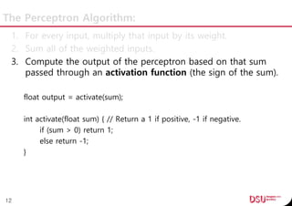
1. For every input, multiply that input by its weight.
2. Sum all of the weighted inputs.
3. Compute the output of the perceptron based on that sum
passed through an activation function (the sign of the sum).
float inputs[] = {12 , 4};
float weights[] = {0.5,-1};
float sum = 0;
for (int i = 0; i < inputs.length; i++) {
sum += inputs[i]*weights[i];
}
11](https://image.slidesharecdn.com/neuralnetwork20161210jintaekseo-170109133919/85/Neural-network-20161210_jintaekseo-11-320.jpg)
![Initialize
Perceptron(int n)
{
mWeightsSize = n;
spWeights = new float[ n ];
//Weights start off random.
for (int i = 0; i < mWeightsSize; i++) {
spWeights[ i ] = random( -1, 1 );
}
}
17](https://image.slidesharecdn.com/neuralnetwork20161210jintaekseo-170109133919/85/Neural-network-20161210_jintaekseo-17-320.jpg)
![Feed forward
int feedforward(float inputs[])
{
float sum = 0;
for (int i = 0; i < mWeightsSize; i++) {
sum += inputs[ i ] * spWeights[ i ];
}
return activate(sum);
}
//Output is a +1 or -1.
int activate(float sum)
{
if (sum > 0) return 1;
else return -1;
}
18](https://image.slidesharecdn.com/neuralnetwork20161210jintaekseo-170109133919/85/Neural-network-20161210_jintaekseo-18-320.jpg)
![Use the Perceptron
Perceptron p = new Perceptron(3);
float point[] = {50,-12,1}; // The input is 3 values: x,y and bias.
int result = p.feedforward(point);
19](https://image.slidesharecdn.com/neuralnetwork20161210jintaekseo-170109133919/85/Neural-network-20161210_jintaekseo-19-320.jpg)
![Learning Constant
NEW WEIGHT = WEIGHT + ERROR * INPUT * LEARNING CONSTANT
With a small learning constant, the weights will be adjusted
slowly, requiring more training time but allowing the network
to make very small adjustments that could improve the
network’s overall accuracy.
float c = 0.01; // learning constant
//Train the network against known data.
void train(float inputs[], int desired) {
int guess = feedforward(inputs);
float error = desired - guess;
for (int i = 0; i < mWeightsSize; i++) {
spWeights[ i ] += c * error * inputs[ i ];
}
}
23](https://image.slidesharecdn.com/neuralnetwork20161210jintaekseo-170109133919/85/Neural-network-20161210_jintaekseo-23-320.jpg)
![Trainer
To train the perceptron, we need a set of inputs with a
known answer.
class Trainer
{
public:
//A "Trainer" object stores the inputs and the correct answer.
float mInputs[ 3 ];
int mAnswer;
void SetData( float x, float y, int a )
{
mInputs[ 0 ] = x;
mInputs[ 1 ] = y;
//Note that the Trainer has the bias input built into its array.
mInputs[ 2 ] = 1;
mAnswer = a;
}24](https://image.slidesharecdn.com/neuralnetwork20161210jintaekseo-170109133919/85/Neural-network-20161210_jintaekseo-24-320.jpg)
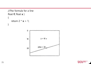
![void Setup()
{
srand( time( 0 ) );
//size( 640, 360 );
spPerceptron.reset( new Perceptron( 3 ) );
// Make 2,000 training points.
for( int i = 0; i < gTrainerSize; i++ ) {
float x = random( -gWidth / 2, gWidth / 2 );
float y = random( -gHeight / 2, gHeight / 2 );
//Is the correct answer 1 or - 1 ?
int answer = 1;
if( y < f( x ) ) answer = -1;
gTraining[ i ].SetData( x, y, answer );
}
}26](https://image.slidesharecdn.com/neuralnetwork20161210jintaekseo-170109133919/85/Neural-network-20161210_jintaekseo-26-320.jpg)
![void Training()
{
for( int i = 0; i < gTrainerSize; i++ ) {
spPerceptron->train( gTraining[ i ].mInputs, gTraining[ i
].mAnswer );
}
}
void main()
{
Setup();
Training();
}
27](https://image.slidesharecdn.com/neuralnetwork20161210jintaekseo-170109133919/85/Neural-network-20161210_jintaekseo-27-320.jpg)
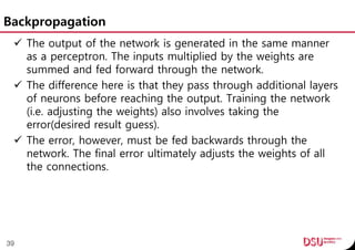
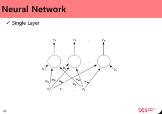
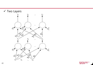
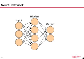
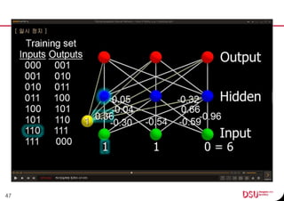
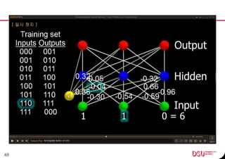

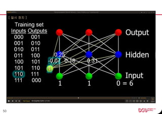
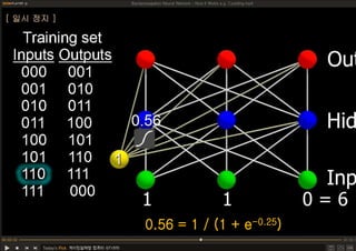
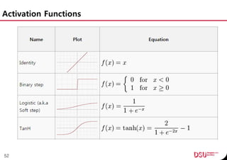

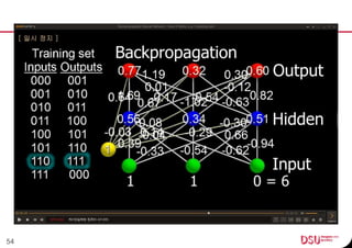
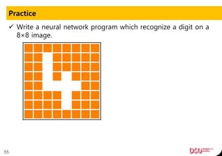


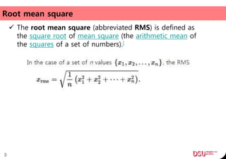
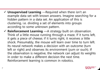
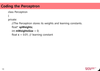
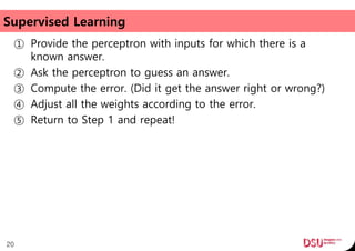
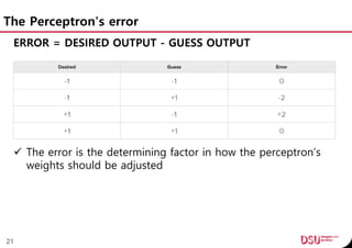
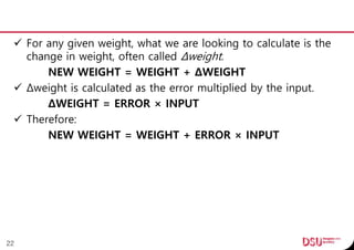
This document discusses neural networks and their applications in mobile game programming. It begins with definitions of standard deviation, root mean square, neurons, dendrites, and axons. It then explains the three main types of machine learning: supervised learning, unsupervised learning, and reinforcement learning. The document also covers standard neural network uses like pattern recognition and control. It provides an in-depth explanation of perceptrons and how they work, including examples of pattern recognition and supervised learning algorithms. Finally, it discusses limitations of single-layer perceptrons and introduces multi-layer perceptrons and backpropagation training.