2
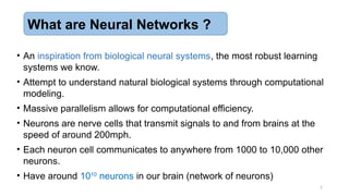
• An inspirationfrom biological neural systems, the most robust learning
systems we know.
• Attempt to understand natural biological systems through computational
modeling.
• Massive parallelism allows for computational efficiency.
• Neurons are nerve cells that transmit signals to and from brains at the
speed of around 200mph.
• Each neuron cell communicates to anywhere from 1000 to 10,000 other
neurons.
• Have around 1010
neurons in our brain (network of neurons)
What are Neural Networks ?
3.
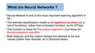
• Neural Netwokis one of the most important learning algorithm in
ML.
• The learned classification model is an algebraic function (or a
set of functions), rather than a boolean function, as for DTrees.
• The function is linear for Perceptron algorithm, non-linear for
Backpropagation algorithm
• Both features and the output classes are allowed to be real
valued (rather than discrete, as in Decision-trees)
3
What are Neural Networks ?
4.
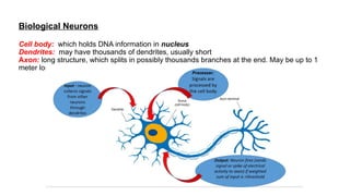
Biological Neurons
Cell body:which holds DNA information in nucleus
Dendrites: may have thousands of dendrites, usually short
Axon: long structure, which splits in possibly thousands branches at the end. May be up to 1
meter long
5.
Biological Neurons
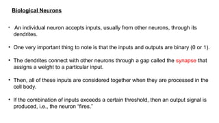
• Anindividual neuron accepts inputs, usually from other neurons, through its
dendrites.
• One very important thing to note is that the inputs and outputs are binary (0 or 1).
• The dendrites connect with other neurons through a gap called the synapse that
assigns a weight to a particular input.
• Then, all of these inputs are considered together when they are processed in the
cell body.
• If the combination of inputs exceeds a certain threshold, then an output signal is
produced, i.e., the neuron “fires.”
6.
6
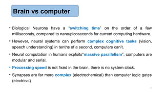
• Biological Neuronshave a “switching time” on the order of a few
milliseconds, compared to nano/picoseconds for current computing hardware.
• However, neural systems can perform complex cognitive tasks (vision,
speech understanding) in tenths of a second, computers can’t.
• Neural computation in humans exploits“massive parallelism”, computers are
modular and serial.
• Processing speed is not fixed in the brain, there is no system clock.
• Synapses are far more complex (electrochemical) than computer logic gates
(electrical)
Brain vs computer
7.
7
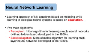
• Learning approachof NN algorithm based on modeling while
learning in biological neural systems is based on adaptation.
• Two main algorithms:
• Perceptron: Initial algorithm for learning simple neural networks
(with no hidden layer) developed in the 1950’s.
• Backpropagation: More complex algorithm for learning multi-
layer neural networks developed in the 1980’s.
Neural Network Learning
8.
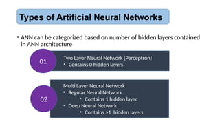
• ANN canbe categorized based on number of hidden layers contained
in ANN architecture
Two Layer Neural Network (Perceptron)
• Contains 0 hidden layers
01
Multi Layer Neural Network
• Regular Neural Network
• Contains 1 hidden layer
• Deep Neural Network
• Contains >1 hidden layers
02
Types of Artificial Neural Networks
9.
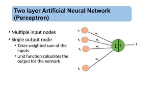
• Multiple inputnodes
• Single output node
• Takes weighted sum of the
inputs
• Unit function calculates the
output for the network
Two layer Artificial Neural Network
(Perceptron)
x1
x2
x3
xn
∑ ?
ŷ
w1
w2
w3
wn
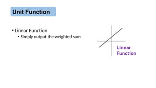
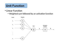
• Linear Function
•Weighted sum followed by an activation function
Unit Function
12.
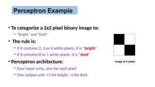
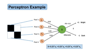
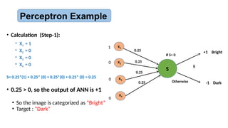
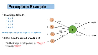
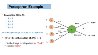
• To categorizea 2x2 pixel binary image to:
• “Bright” and “Dark”
• The rule is:
• If it contains 2, 3 or 4 white pixels, it is “bright”
• If it contains 0 or 1 white pixels, it is “dark”
• Perceptron architecture:
• Four input units, one for each pixel
• One output unit: +1 for bright, -1 for dark
Perceptron Example
Image of 4 pixels
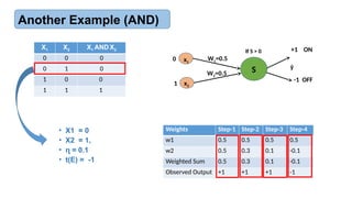
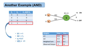
Another Example (AND)
x1
x2
Sŷ
W1=0.5
W2=0.5
+1 ON
-1 OFF
If S > 0
0
1
X1 X2 X1 AND X2
0 0 0
0 1 0
1 0 0
1 1 1
Weights Step-1 Step-2 Step-3 Step-4
w1 0.5 0.5 0.5 0.5
w2 0.5 0.3 0.1 -0.1
Weighted Sum 0.5 0.3 0.1 -0.1
Observed Output +1 +1 +1 -1
• X1 = 0
• X2 = 1,
• = 0.1
ɳ
• t(E) = -1
21.
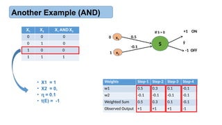
Another Example (AND)
x1
x2
Sŷ
0.5
-0.1
+1 ON
-1 OFF
If S > 0
0
1
X1 X2 X1 AND X2
0 0 0
0 1 0
1 0 0
1 1 1
Weights Step-1 Step-2 Step-3 Step-4
w1 0.5 0.3 0.1 -0.1
w2 -0.1 -0.1 -0.1 -0.1
Weighted Sum 0.5 0.3 0.1 -0.1
Observed Output +1 +1 +1 -1
• X1 = 1
• X2 = 0,
• = 0.1
ɳ
• t(E) = -1
22.
Another Example (AND)
x1
x2
Sŷ
-0.1
-0.1
+1 ON
-1 OFF
If S > 0
0
1
X1 X2 X1 AND X2
0 0 0
0 1 0
1 0 0
1 1 1
Weights Step-1 Step-2
w1 -0.1 0.1
w2 -0.1 0.1
Weighted Sum -0.2 0.2
Observed Output - 1 +1
• X1 = 1
• X2 = 1,
• = 0.1
ɳ
• t(E) = +1
23.
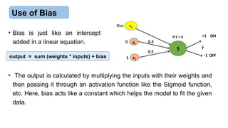
Use of Bias
x1
x2
Sŷ
0.5
0.5
+1 ON
-1 OFF
If S > 0
0
1
• Bias is just like an intercept
added in a linear equation.
output = sum (weights * inputs) + bias
• The output is calculated by multiplying the inputs with their weights and
then passing it through an activation function like the Sigmoid function,
etc. Here, bias acts like a constant which helps the model to fit the given
data.
x0
Bias
24.
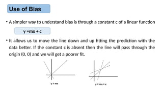
Use of Bias
•A simpler way to understand bias is through a constant c of a linear function
y =mx + c
• It allows us to move the line down and up fitting the prediction with the
data better. If the constant c is absent then the line will pass through the
origin (0, 0) and we will get a poorer fit.
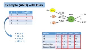
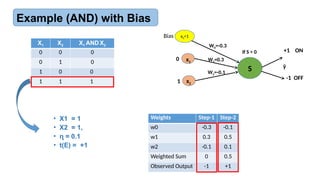
X1 X2 X1AND X2
0 0 0
0 1 0
1 0 0
1 1 1
Weights Step-1 Step-2
w0 -0.1 -0.3
w1 0.5 0.3
w2 -0.1 -0.1
Weighted Sum 0.4 0
Observed Output +1 -1
• X1 = 1
• X2 = 0,
• = 0.1
ɳ
• t(E) = -1
x1
x2
S ŷ
W1=0.5
W2=-0.1
+1 ON
-1 OFF
If S > 0
0
1
x0=1
Bias
W0=-0.1
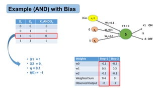
Example (AND) with Bias
27.
X1 X2 X1AND X2
0 0 0
0 1 0
1 0 0
1 1 1
Weights Step-1 Step-2
w0 -0.3 -0.1
w1 0.3 0.5
w2 -0.1 0.1
Weighted Sum 0 0.5
Observed Output -1 +1
• X1 = 1
• X2 = 1,
• = 0.1
ɳ
• t(E) = +1
x1
x2
S ŷ
W1=0.3
W2=-0.1
+1 ON
-1 OFF
If S > 0
0
1
x0=1
Bias
W0=-0.3
Example (AND) with Bias
28.
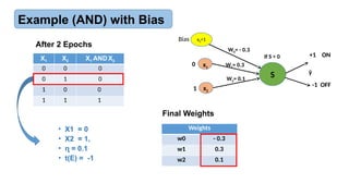
X1 X2 X1AND X2
0 0 0
0 1 0
1 0 0
1 1 1
Weights
w0 - 0.3
w1 0.3
w2 0.1
• X1 = 0
• X2 = 1,
• = 0.1
ɳ
• t(E) = -1
x1
x2
S ŷ
W1= 0.3
W2= 0.1
+1 ON
-1 OFF
If S > 0
0
1
x0=1
Bias
W0= - 0.3
After 2 Epochs
Final Weights
Example (AND) with Bias
29.
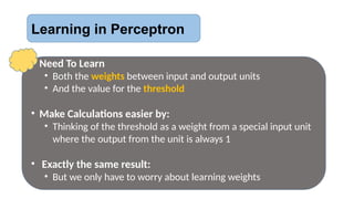
Learning in Perceptron
•Need To Learn
• Both the weights between input and output units
• And the value for the threshold
• Make Calculations easier by:
• Thinking of the threshold as a weight from a special input unit
where the output from the unit is always 1
• Exactly the same result:
• But we only have to worry about learning weights
30.
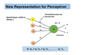
New Representation forPerceptron
Special input, which is
always 1
x1
x2
xn
S
ŷ
w1
w2
wn
1
w0
If S > 0
+1
-1
Otherwise
Threshold function has
become this
S= w0 + w1*x1 + w2*x2 . . . . . . . wn*xn
31.
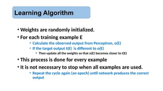
Learning Algorithm
• Weightsare randomly initialized.
• For each training example E
• Calculate the observed output from Perceptron, o(E)
• If the target output t(E) is different to o(E)
• Then update all the weights so that o(E) becomes closer to t(E)
• This process is done for every example
• It is not necessary to stop when all examples are used.
• Repeat the cycle again (an epoch) until network produces the correct
output
32.
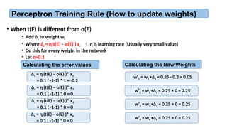
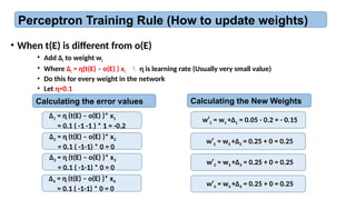
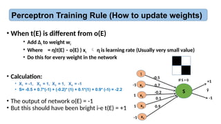
Perceptron Training Rule(How to update weights)
• When t(E) is different from o(E)
• Add ∆i to weight wi
• Where = ɳ(t(E) – o(E) ) xi ɳ is learning rate (Usually very small value)
• Do this for every weight in the network
1
x1
x2
x4
S ŷ
0.7
-0.2
0.9
x3
-0.5
0.1
• Calculation:
• X1 = -1, X2 = 1, X3 = 1, X4 = -1
• S= -0.5 + 0.7*(-1) + (-0.2)* (1) + 0.1*(1) + 0.9* (-1) = -2.2
• The output of network o(E) = -1
• But this should have been bright i-e t(E) = +1
+1
-1
If S > 0
-1
1
1
-1
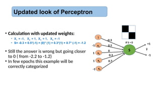
Updated look ofPerceptron
1
x1
x2
x4
S ŷ
0.5
0
0.7
x3
-0.3
0.3
+1
-1
If S > 0
• Calculation with updated weights:
• X1 = -1, X2 = 1, X3 = 1, X4 = -1
• S= -0.3 + 0.5*(-1) + (0)* (1) + 0.3*(1) + 0.7* (-1) = -1.2
• Still the answer is wrong but going closer
to 0 ( from -2.2 to -1.2)
• In few epochs this example will be
correctly categorized
-1
1
1
-1
35.
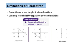
Limitations of Perceptron
•Cannot learn some simple Boolean functions
• Can only learn linearly separable Boolean functions


![AI-Lecture-11[Neural Network] updated.pptx](https://cdn.slidesharecdn.com/ss_thumbnails/ai-lecture-11neuralnetworkupdated-251220065329-186ba89b-thumbnail.jpg?width=640&height=640&fit=bounds)


