The document provides an introduction to neural networks, contrasting biological and artificial neurons and explaining key algorithms such as perceptron and backpropagation. It details the structure and functioning of single-layer and multi-layer neural networks, highlighting how weights are adjusted during training to improve predictions. The text also addresses the limitations of perceptrons, particularly their ability to only solve linearly separable problems.

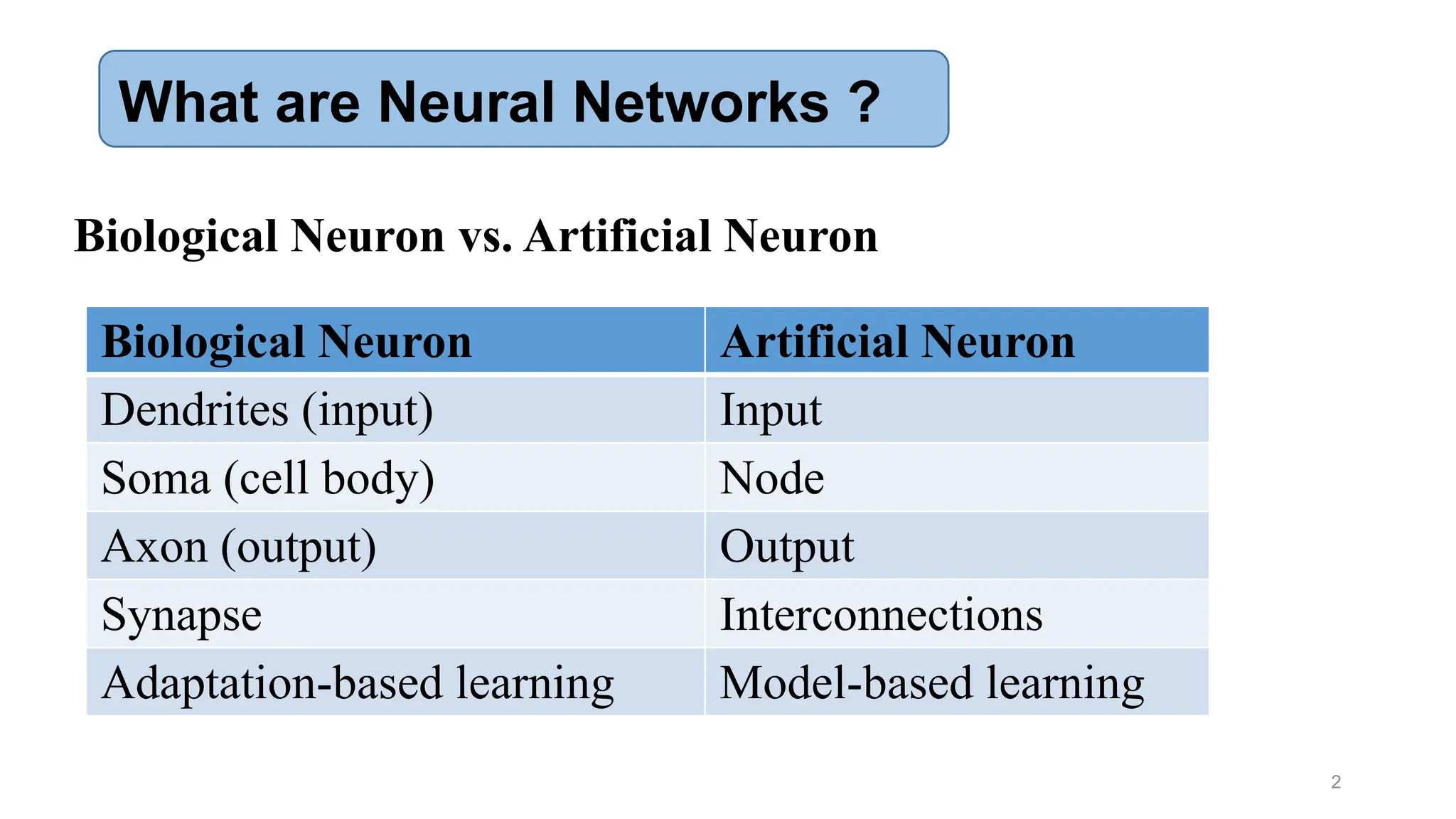
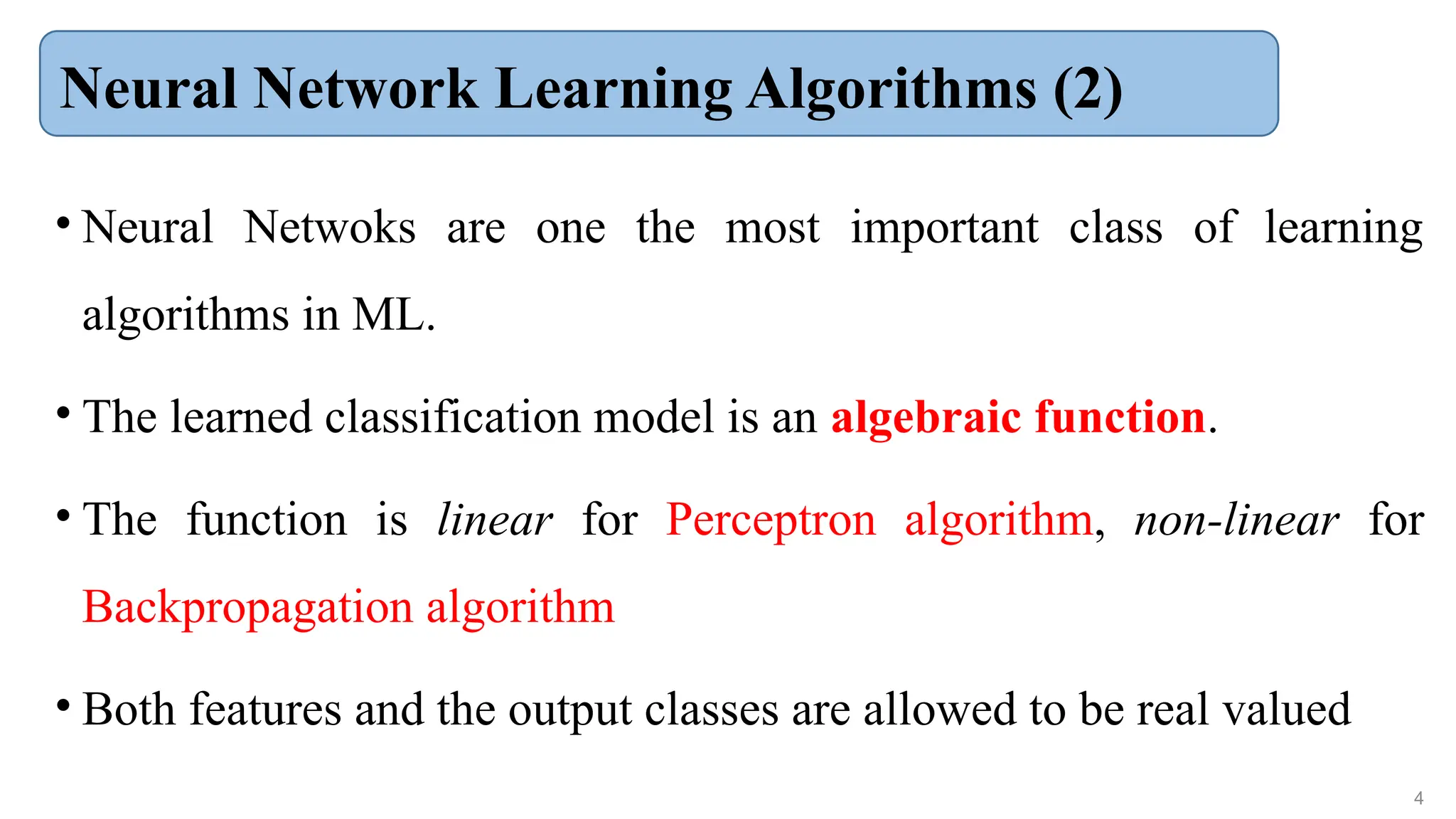
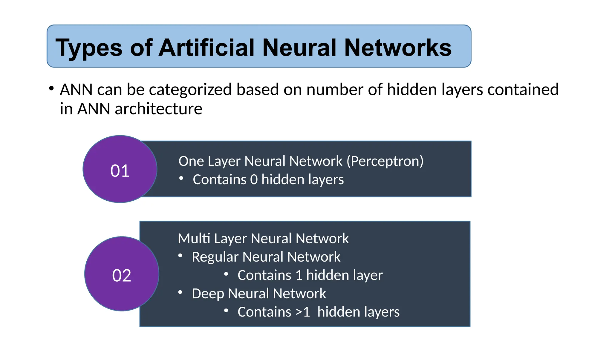
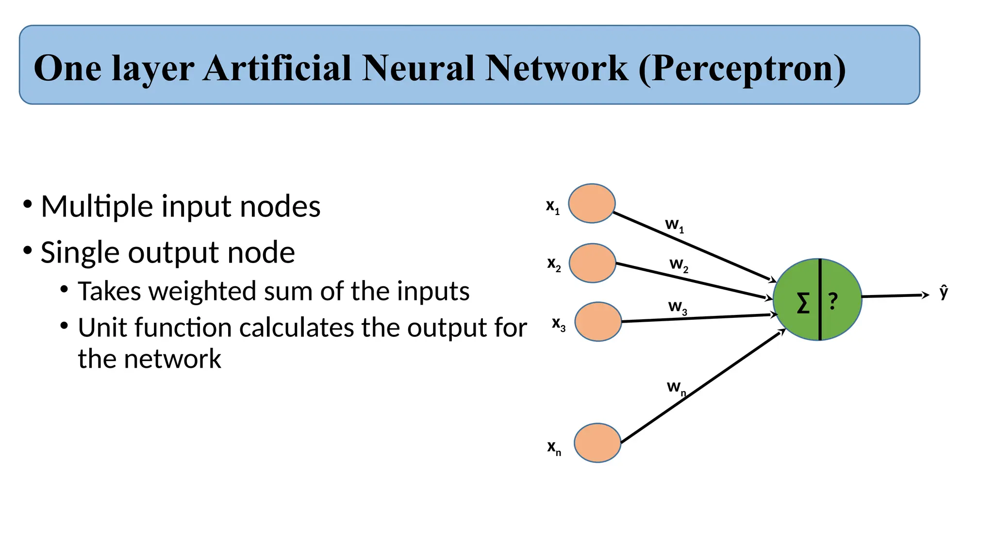
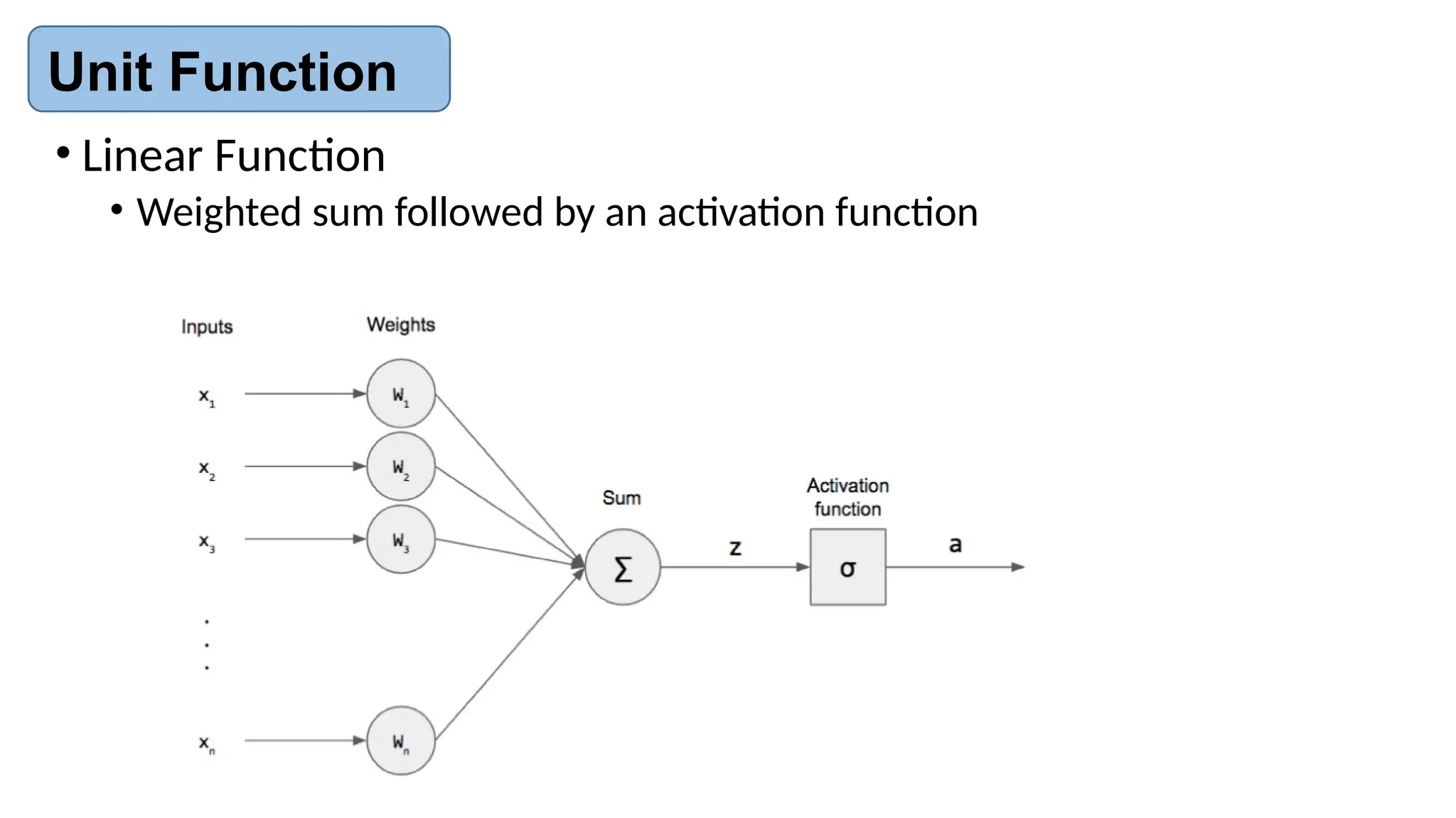
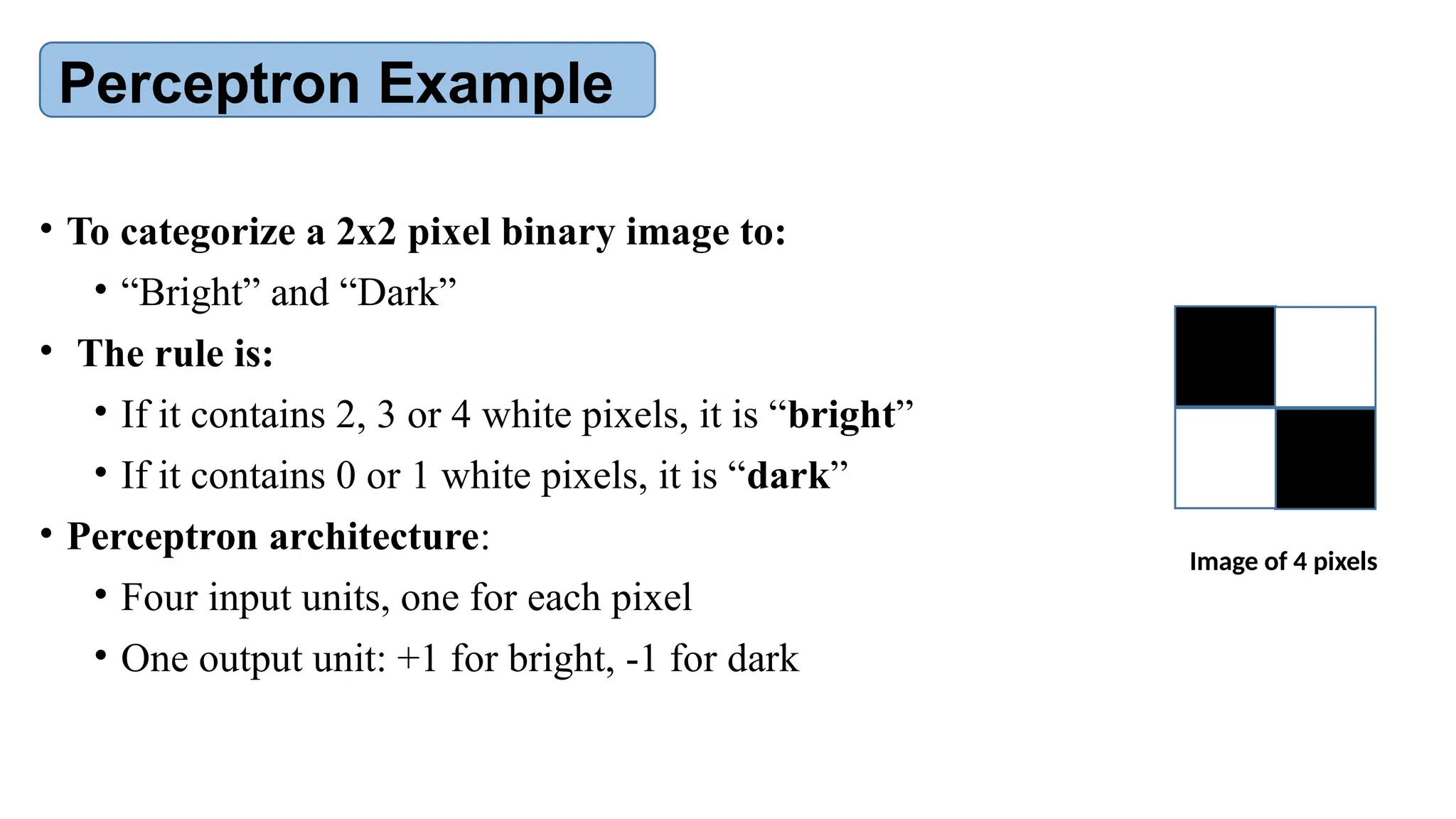
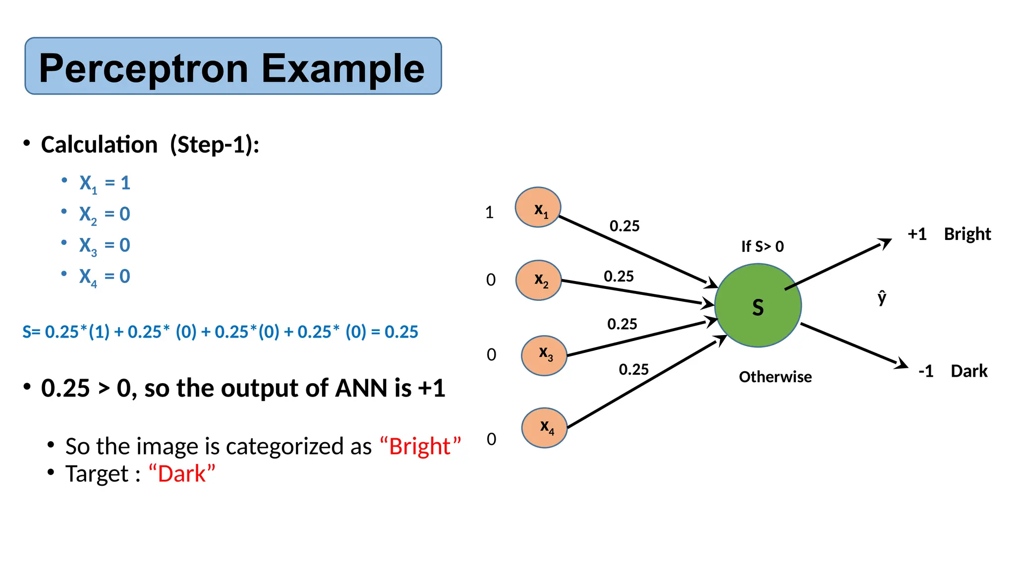
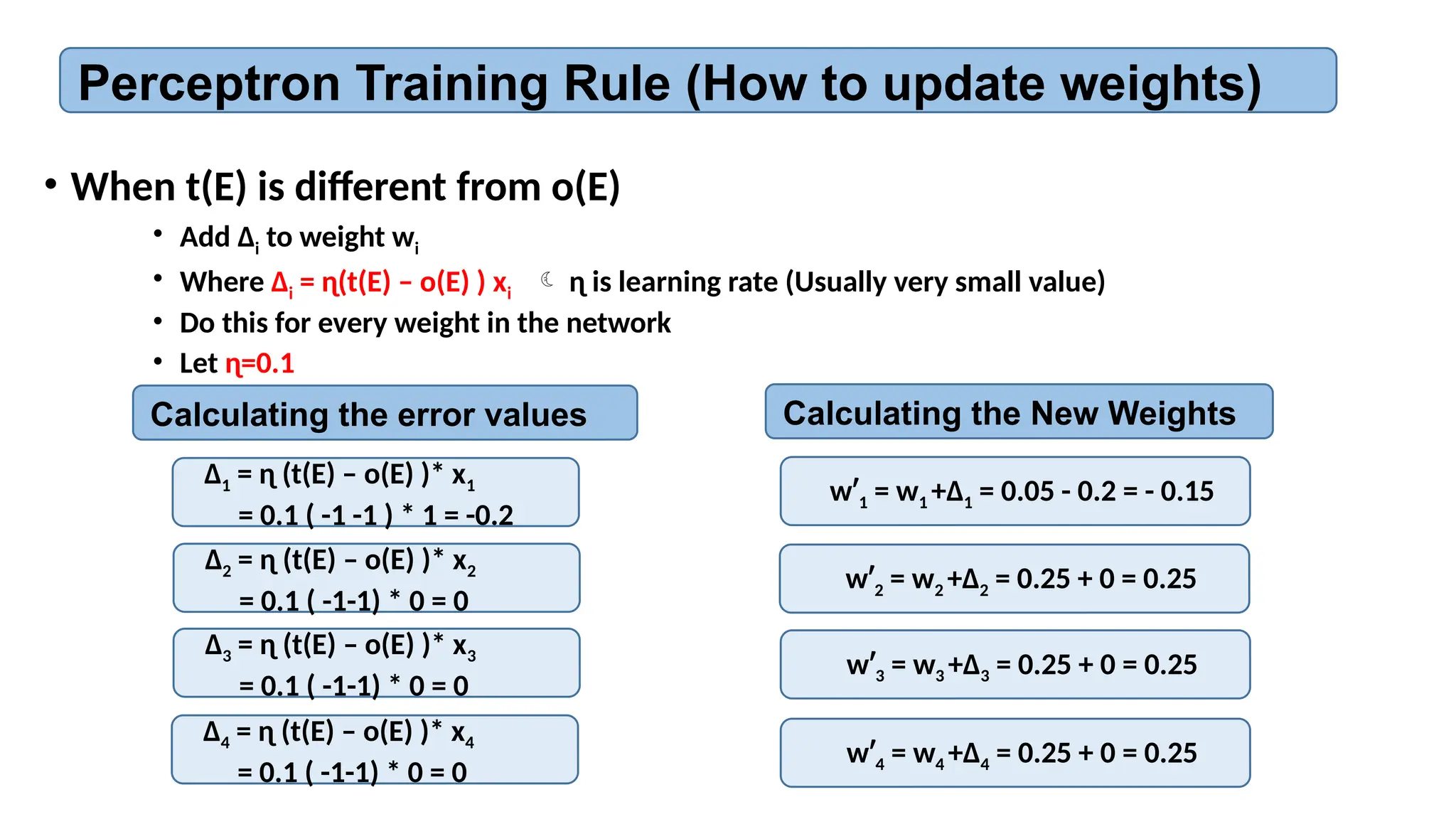
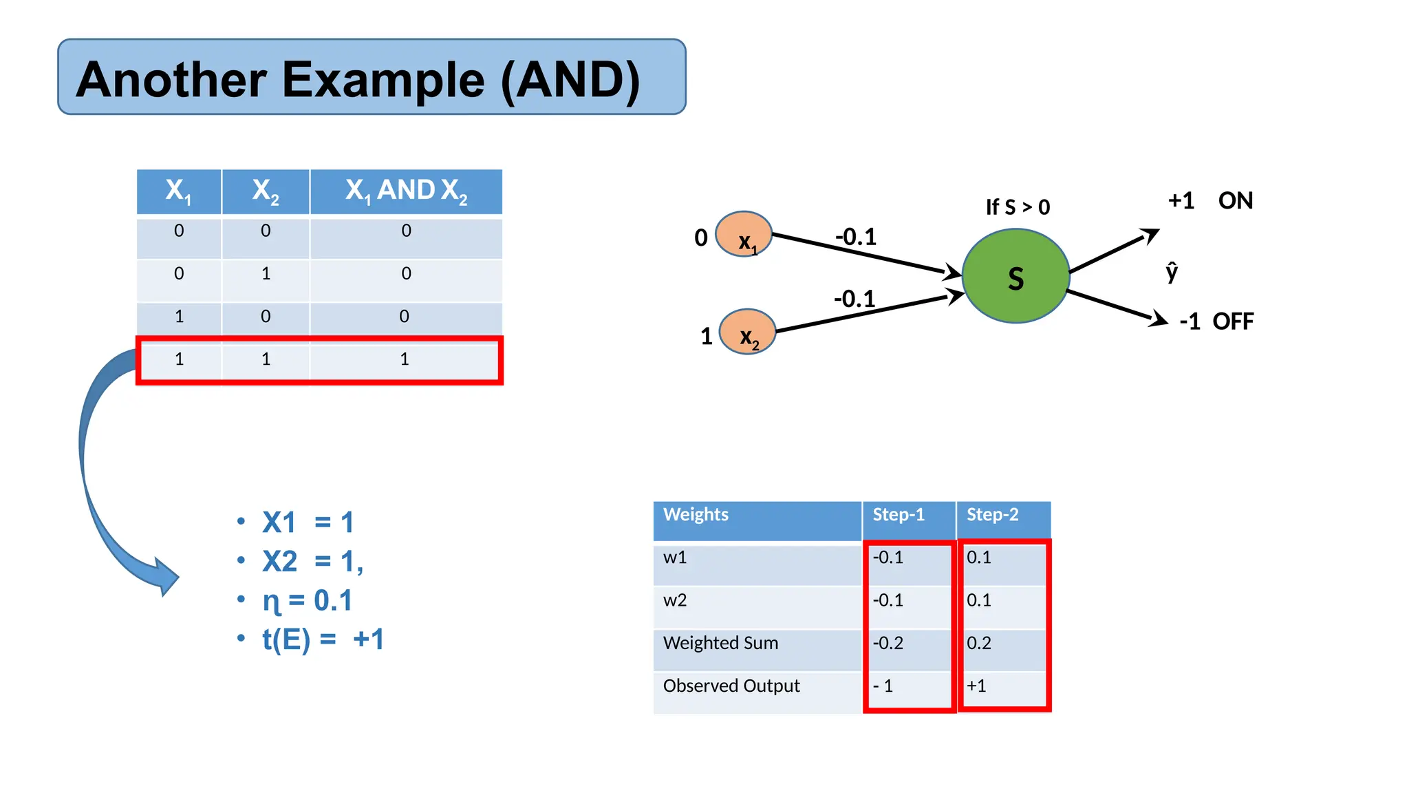
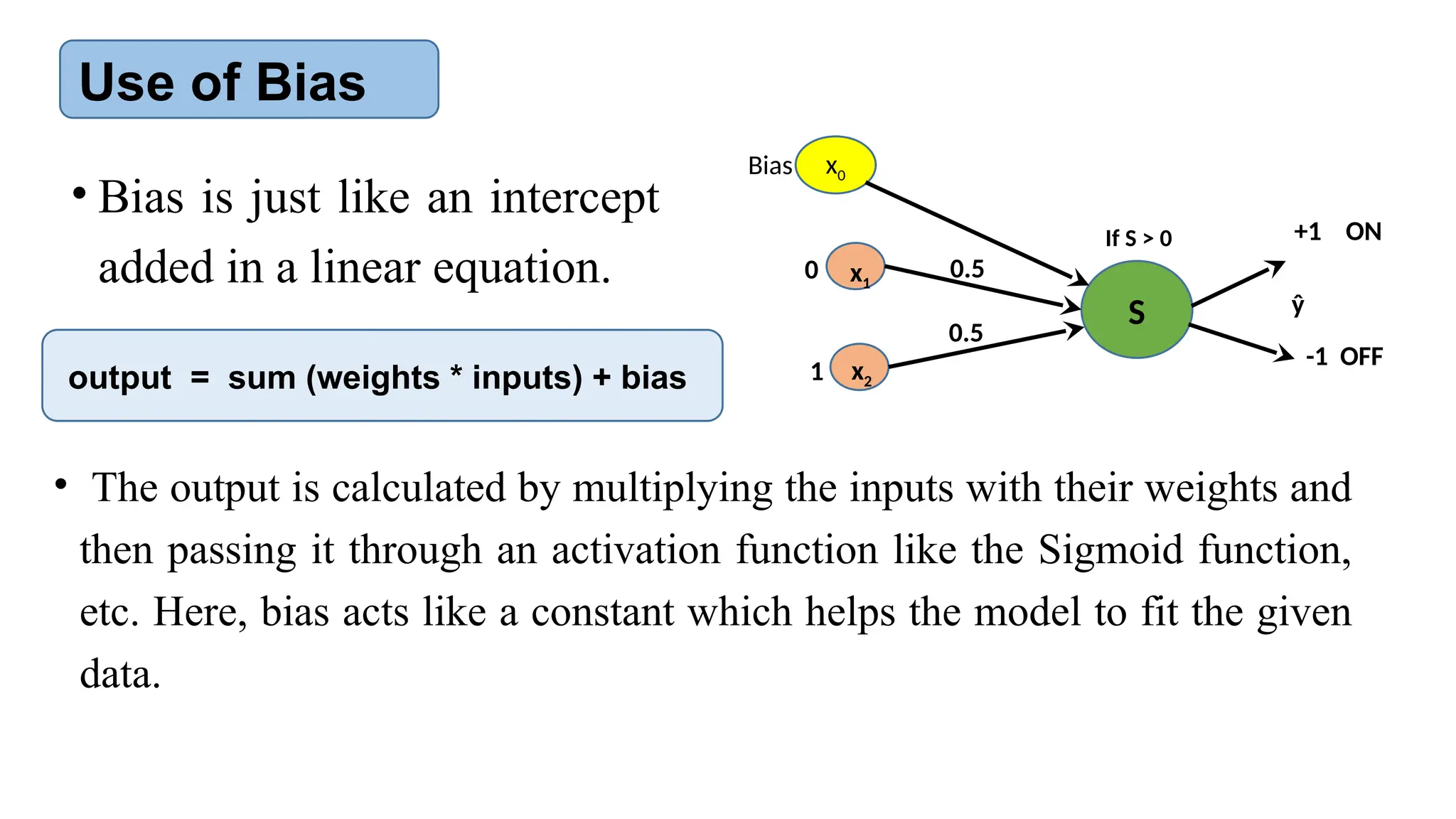
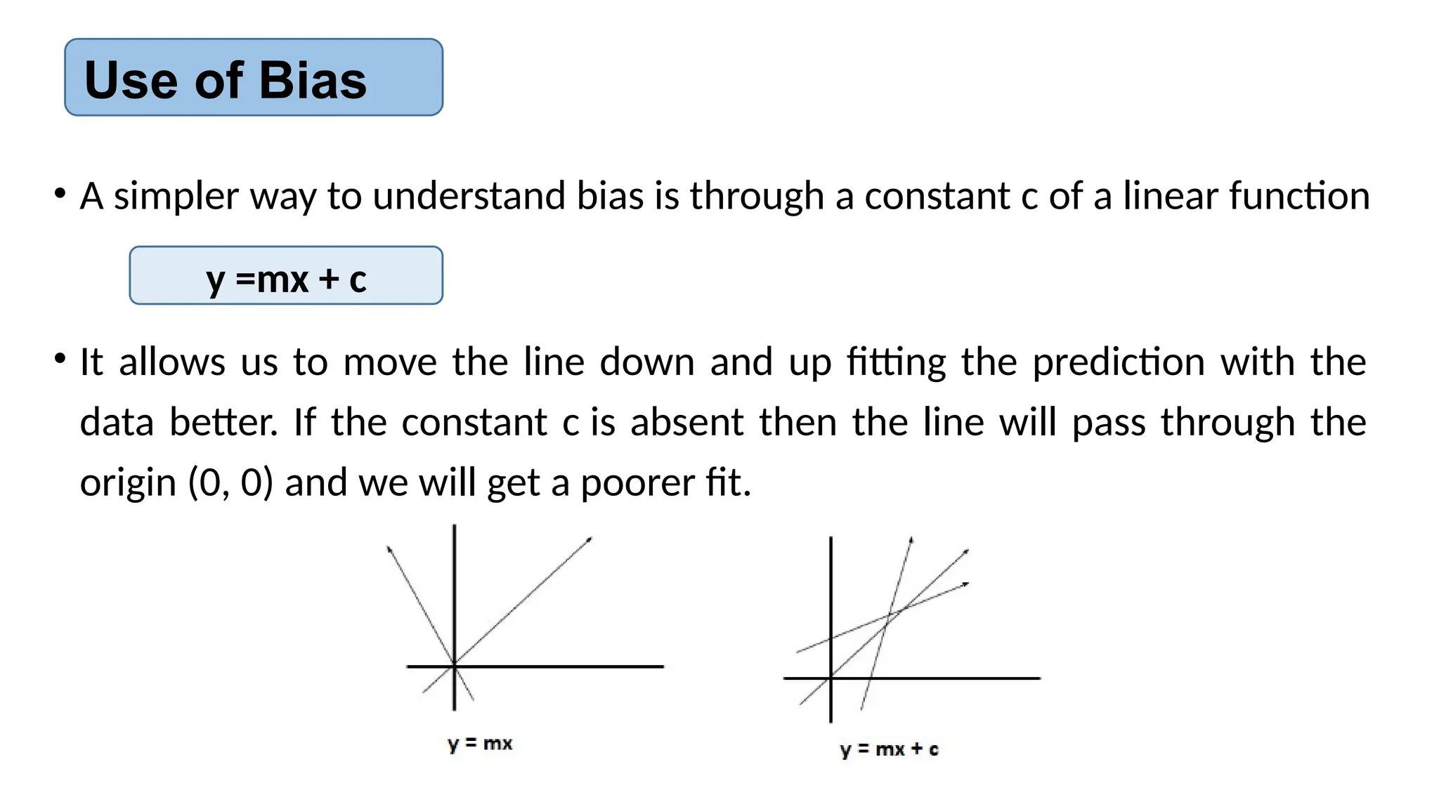
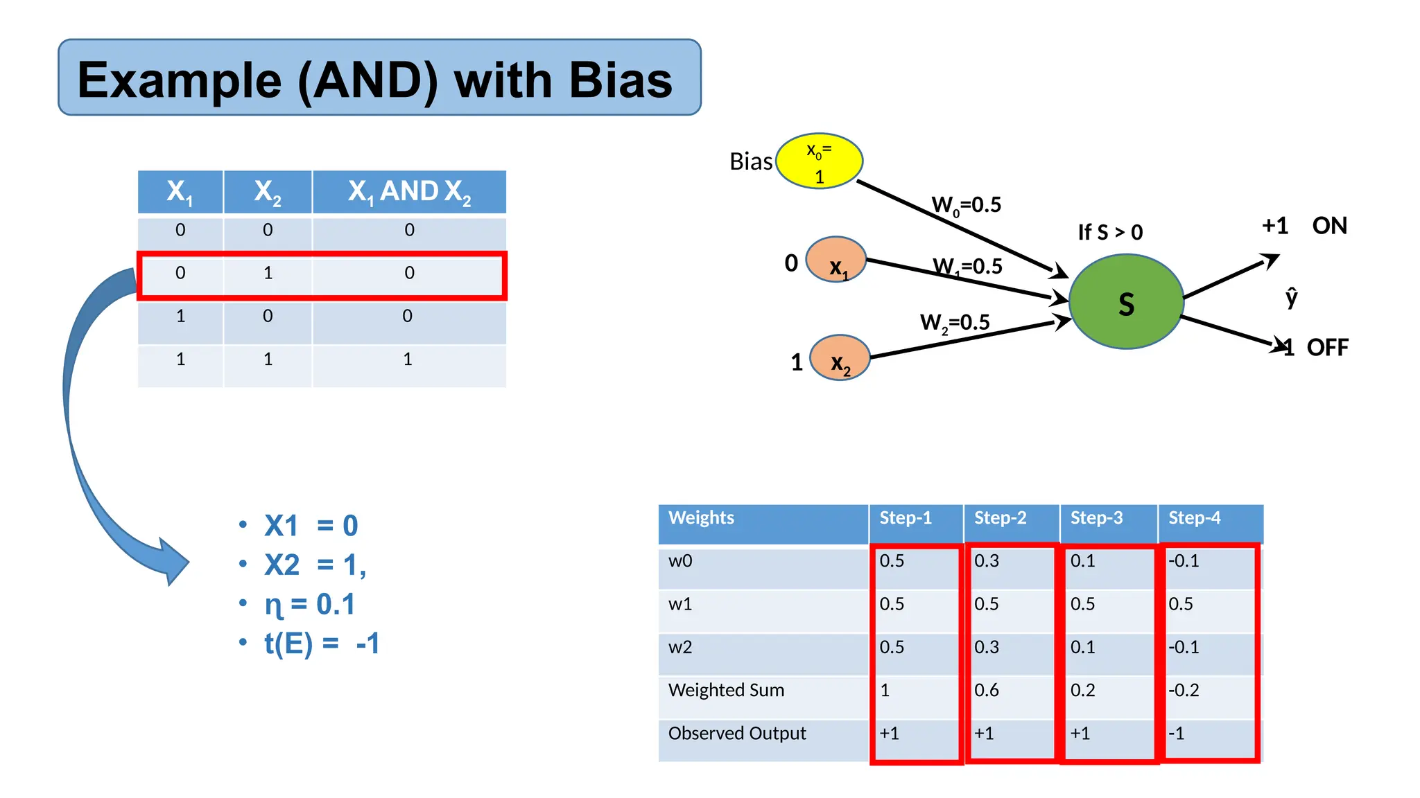
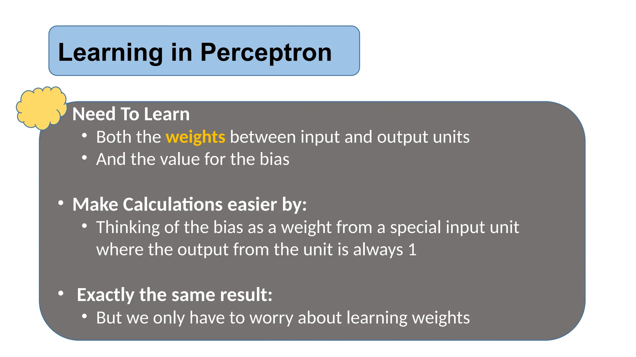
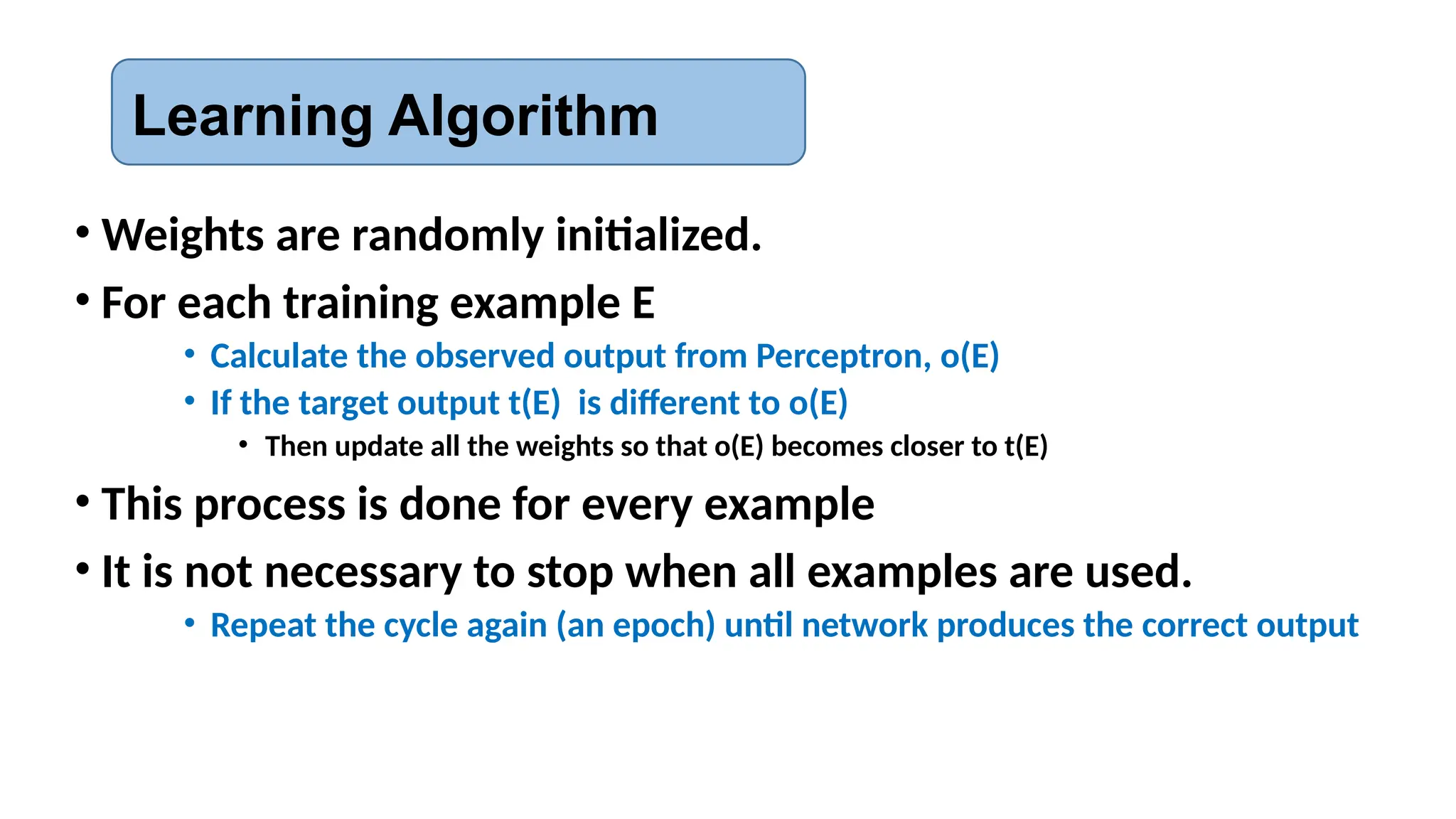
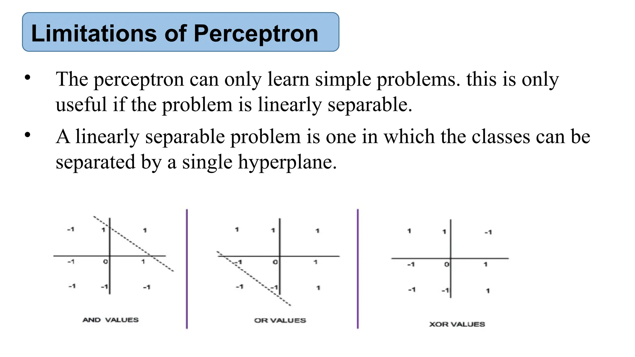
1. 1
Lecture-02: Introduction to Neural
Networks

2. 2
Biological Neuron vs. Artificial Neuron
What are Neural Networks ?
Biological Neuron Artificial Neuron
Dendrites (input) Input
Soma (cell body) Node
Axon (output) Output
Synapse Interconnections
Adaptation-based learning Model-based learning

3. 3
• Two main algorithms:
• Perceptron: Initial algorithm for learning simple neural
networks (with no hidden layer) developed in the 1950’s.
• Backpropagation: More complex algorithm for learning multi-
layer neural networks developed in the 1980’s.
Neural Network Learning Algorithms (1)

4. • Neural Netwoks are one the most important class of learning
algorithms in ML.
• The learned classification model is an algebraic function.
• The function is linear for Perceptron algorithm, non-linear for
Backpropagation algorithm
• Both features and the output classes are allowed to be real valued
4
Neural Network Learning Algorithms (2)

5. Perceptron: The First Neural Network

6. • ANN can be categorized based on number of hidden layers contained
in ANN architecture
One Layer Neural Network (Perceptron)
• Contains 0 hidden layers
01
Multi Layer Neural Network
• Regular Neural Network
• Contains 1 hidden layer
• Deep Neural Network
• Contains >1 hidden layers
02
Types of Artificial Neural Networks

7. • Multiple input nodes
• Single output node
• Takes weighted sum of the inputs
• Unit function calculates the output for
the network
One layer Artificial Neural Network (Perceptron)
x1
x2
x3
xn
∑ ? ŷ
w1
w2
w3
wn

8. • Linear Function
• Simply output the weighted sum
Unit Function

9. • Linear Function
• Weighted sum followed by an activation function
Unit Function

10. • To categorize a 2x2 pixel binary image to:
• “Bright” and “Dark”
• The rule is:
• If it contains 2, 3 or 4 white pixels, it is “bright”
• If it contains 0 or 1 white pixels, it is “dark”
• Perceptron architecture:
• Four input units, one for each pixel
• One output unit: +1 for bright, -1 for dark
Perceptron Example
Image of 4 pixels

11. x1
x2
x3
x4
S ŷ
0.25
0.25
0.25
0.25
Pixel 1
Pixel 4
Pixel 3
Pixel 2
+1 Bright
If S> -0.1
-1 Dark
S= 0.25*x1 + 0.25*x2 + 0.25*x3 + 0.25*x4
Otherwise
Perceptron Example

12. • Calculation (Step-1):
• X1 = 1
• X2 = 0
• X3 = 0
• X4 = 0
S= 0.25*(1) + 0.25* (0) + 0.25*(0) + 0.25* (0) = 0.25
• 0.25 > 0, so the output of ANN is +1
• So the image is categorized as “Bright”
• Target : “Dark”
Perceptron Example
x1
x2
x3
x4
S ŷ
0.25
0.25
0.25
0.25
1
0
0
0
+1 Bright
If S> 0
-1 Dark
Otherwise

13. Perceptron Training Rule (How to update weights)
• When t(E) is different from o(E)
• Add ∆i to weight wi
• Where ∆i = ɳ(t(E) – o(E) ) xi  ɳ is learning rate (Usually very small value)
• Do this for every weight in the network
• Let ɳ=0.1
∆1 = ɳ (t(E) – o(E) )* x1
= 0.1 ( -1-1) * 1 = -0.2
∆2 = ɳ (t(E) – o(E) )* x2
= 0.1 ( -1-1) * 0 = 0
∆3 = ɳ (t(E) – o(E) )* x3
= 0.1 ( -1-1) * 0 = 0
∆4 = ɳ (t(E) – o(E) )* x4
= 0.1 ( -1-1) * 0 = 0
wʹ1 = w1 +∆1 = 0.25 - 0.2 = 0.05
wʹ2 = w2 +∆2 = 0.25 + 0 = 0.25
wʹ3 = w3 +∆3 = 0.25 + 0 = 0.25
wʹ4 = w4 +∆4 = 0.25 + 0 = 0.25
Calculating the error values Calculating the New Weights

14. • Calculation (Step-2):
• X1 = 1
• X2 = 0
• X3 = 0
• X4 = 0
S= 0.05*(1) + 0.25* (0) + 0.25*(0) + 0.25* (0) = 0.05
• 0.05 > 0, so the output of ANN is +1
• So the image is categorized as “Bright”
• Target : “Dark”
Perceptron Example
x1
x2
x3
x4
S ŷ
0.05
0.25
0.25
0.25
1
0
0
0
+1 Bright
If S> 0
-1 Dark
Otherwise

15. Perceptron Training Rule (How to update weights)
• When t(E) is different from o(E)
• Add ∆i to weight wi
• Where ∆i = ɳ(t(E) – o(E) ) xi  ɳ is learning rate (Usually very small value)
• Do this for every weight in the network
• Let ɳ=0.1
∆1 = ɳ (t(E) – o(E) )* x1
= 0.1 ( -1 -1 ) * 1 = -0.2
∆2 = ɳ (t(E) – o(E) )* x2
= 0.1 ( -1-1) * 0 = 0
∆3 = ɳ (t(E) – o(E) )* x3
= 0.1 ( -1-1) * 0 = 0
∆4 = ɳ (t(E) – o(E) )* x4
= 0.1 ( -1-1) * 0 = 0
wʹ1 = w1 +∆1 = 0.05 - 0.2 = - 0.15
wʹ2 = w2 +∆2 = 0.25 + 0 = 0.25
wʹ3 = w3 +∆3 = 0.25 + 0 = 0.25
wʹ4 = w4 +∆4 = 0.25 + 0 = 0.25
Calculating the error values Calculating the New Weights

16. • Calculation (Step-3):
• X1 = 1
• X2 = 0
• X3 = 0
• X4 = 0
S= - 0.15*(1) + 0.25* (0) + 0.25*(0) + 0.25* (0) = - 0.15
• - 0.15 < 0, so the output of ANN is -1
• So the image is categorized as “Dark”
• Target : “Dark”
Perceptron Example
x1
x2
x3
x4
S ŷ
-0.15
0.2
5
0.2
5
0.2
5
1
0
0
0
+1 Bright
If S> 0
-1 Dark
Otherwise

17. Another Example (AND)
x1
x2
S ŷ
W1=0.5
W2=0.5
+1 ON
-1 OFF
If S > 0
0
1
X1 X2 X1 AND X2
0 0 0
0 1 0
1 0 0
1 1 1
Weights Step-1 Step-2 Step-3 Step-4
w1 0.5 0.5 0.5 0.5
w2 0.5 0.3 0.1 -0.1
Weighted Sum 0.5 0.3 0.1 -0.1
Observed Output +1 +1 +1 -1
• X1 = 0
• X2 = 1,
• = 0.1
ɳ
• t(E) = -1

18. Another Example (AND)
x1
x2
S ŷ
0.5
-0.1
+1 ON
-1 OFF
If S > 0
0
1
X1 X2 X1 AND X2
0 0 0
0 1 0
1 0 0
1 1 1
Weights Step-1 Step-2 Step-3 Step-4
w1 0.5 0.3 0.1 -0.1
w2 -0.1 -0.1 -0.1 -0.1
Weighted Sum 0.5 0.3 0.1 -0.1
Observed Output +1 +1 +1 -1
• X1 = 1
• X2 = 0,
• = 0.1
ɳ
• t(E) = -1

19. Another Example (AND)
x1
x2
S ŷ
-0.1
-0.1
+1 ON
-1 OFF
If S > 0
0
1
X1 X2 X1 AND X2
0 0 0
0 1 0
1 0 0
1 1 1
Weights Step-1 Step-2
w1 -0.1 0.1
w2 -0.1 0.1
Weighted Sum -0.2 0.2
Observed Output - 1 +1
• X1 = 1
• X2 = 1,
• = 0.1
ɳ
• t(E) = +1

20. Use of Bias
x1
x2
S ŷ
0.5
0.5
+1 ON
-1 OFF
If S > 0
0
1
• Bias is just like an intercept
added in a linear equation.
output = sum (weights * inputs) + bias
• The output is calculated by multiplying the inputs with their weights and
then passing it through an activation function like the Sigmoid function,
etc. Here, bias acts like a constant which helps the model to fit the given
data.
x0
Bias

21. Use of Bias
• A simpler way to understand bias is through a constant c of a linear function
y =mx + c
• It allows us to move the line down and up fitting the prediction with the
data better. If the constant c is absent then the line will pass through the
origin (0, 0) and we will get a poorer fit.

22. Example (AND) with Bias
X1 X2 X1 AND X2
0 0 0
0 1 0
1 0 0
1 1 1
Weights Step-1 Step-2 Step-3 Step-4
w0 0.5 0.3 0.1 -0.1
w1 0.5 0.5 0.5 0.5
w2 0.5 0.3 0.1 -0.1
Weighted Sum 1 0.6 0.2 -0.2
Observed Output +1 +1 +1 -1
• X1 = 0
• X2 = 1,
• = 0.1
ɳ
• t(E) = -1
x1
x2
S ŷ
W1=0.5
W2=0.5
+1 ON
-1 OFF
If S > 0
0
1
x0=
1
Bias
W0=0.5

23. X1 X2 X1 AND X2
0 0 0
0 1 0
1 0 0
1 1 1
Weights Step-1 Step-2
w0 -0.1 -0.3
w1 0.5 0.3
w2 -0.1 -0.1
Weighted Sum 0.4 0
Observed Output +1 -1
• X1 = 1
• X2 = 0,
• = 0.1
ɳ
• t(E) = -1
x1
x2
S ŷ
W1=0.
5
W2=-
0.1
+1 ON
-1 OFF
If S > 0
0
1
x0=
1
Bias
W0=-0.1
Example (AND) with Bias

24. X1 X2 X1 AND X2
0 0 0
0 1 0
1 0 0
1 1 1
Weights Step-1 Step-2
w0 -0.3 -0.1
w1 0.3 0.5
w2 -0.1 0.1
Weighted Sum 0 0.5
Observed Output -1 +1
• X1 = 1
• X2 = 1,
• = 0.1
ɳ
• t(E) = +1
x1
x2
S ŷ
W1=0.
3
W2=-
0.1
+1 ON
-1 OFF
If S > 0
0
1
x0=
1
Bias
W0=-0.3
Example (AND) with Bias

25. X1 X2 X1 AND X2
0 0 0
0 1 0
1 0 0
1 1 1
Weights
w0 - 0.3
w1 0.3
w2 0.1
• X1 = 0
• X2 = 1,
• = 0.1
ɳ
• t(E) = -1
x1
x2
S ŷ
W1=
0.3
W2=
0.1
+1 ON
-1 OFF
If S > 0
0
1
x0=
1
Bias
W0= -
0.3
After 2 Epochs
Final Weights
Example (AND) with Bias

26. Learning in Perceptron
• Need To Learn
• Both the weights between input and output units
• And the value for the bias
• Make Calculations easier by:
• Thinking of the bias as a weight from a special input unit
where the output from the unit is always 1
• Exactly the same result:
• But we only have to worry about learning weights

27. New Representation for Perceptron
Special input, which is
always 1
x1
x2
xn
S ŷ
w1
w2
wn
1
w0
If S > 0
+1
-1
Otherwis
e
Threshold function has
become this
S= w0 + w1*x1 + w2*x2 . . . . . . . wn*xn

28. Learning Algorithm
• Weights are randomly initialized.
• For each training example E
• Calculate the observed output from Perceptron, o(E)
• If the target output t(E) is different to o(E)
• Then update all the weights so that o(E) becomes closer to t(E)
• This process is done for every example
• It is not necessary to stop when all examples are used.
• Repeat the cycle again (an epoch) until network produces the correct output

29. Limitations of Perceptron
• by a single hyperplane.
• The perceptron can only learn simple problems. this is only
useful if the problem is linearly separable.
• A linearly separable problem is one in which the classes can be
separated by a single hyperplane.

30. Any Questions?