1. Slope = -0.3421
R² = 0.9816
0
20
40
60
80
100
120
0 50 100 150 200 250
#Events>M7per1000yrs
Sigma (MPa)
Normal Stress Sensitivity
Abstract
As part of the 2016 Undergraduate Studies in Earthquake Information Technology (USEIT) internship program, students worked in collaborative groups to tackle unsolved problems in earthquake information technology presented in the form of a Grand Challenge. Earthquake
forecasting was the overall theme of this year’s Grand Challenge. The USEIT High Performance Computing (HPC) Team was challenged to simulate long catalogs of California’s seismic activity on a supercomputer. The team used a physics-based earthquake simulator, the
Rate-State earthQuake Simulator (RSQSim). The students ran the simulations on the Blue Waters system at the University of Illinois, one of the most powerful open-science supercomputers in the world. To configure an RSQSim simulation, a series of initial physical
parameters must be specified, including initial normal and shear stresses, rate- and state-friction parameters, and earthquake slip rate. The HPC Team studied the effects of these parameters on simulated catalogs. Each team member ran several short simulations (25,000
simulated years) with different input parameters and then compared the catalogs with the Uniform California Earthquake Rupture Forecast Version 3 (UCERF3) to determine which parameter set produced the best match. The HPC team also utilized the R Programing
Language, a language commonly used by statisticians as well as data miners, in order to analyze the results of each catalog. Varying the parameter sets produced drastic changes in the catalogs generated. With the help of the Probabilistic Forecasting Team, the HPC Team
compared each of the short catalogs with multiple aspects of the UCERF3 data. Of the seventeen short catalogs generated, Sigma High had less than a 2% difference from UCERF3 in the recurrence interval of events M ≥ 7 on the Southern San Andreas Fault, which indicated
that the parameter set was the best representation of an earth-like system. Based on this information, the team extended the catalog to 530,000 years in order to create a more comprehensive dataspace for earthquake forecasting. The USEIT interns used these catalogs to
answer probabilistic questions posted in the Grand Challenge and generate simulator-based forecasts for the San Andreas Fault System.
2016 USEIT: Physics-Based Simulations Using High Performance Computing
Morgan Bent1
, David Fu1
, Hernan Lopez2
, Spencer Ortega3
, Kevin Scroggins3
, Scott Callaghan4
, Jacqui Gilchrist4
, Mark Benthien4
, Jozi Pearson4
, Thomas Jordan4
(1) University of Southern California, (2) California Polytechnic State University Pomona, (3) Pasadena City College, (4) Southern California Earthquake Center
Parameter Sensitivity
This figure illustrates the sensitivity of the rate of large events (M ≥ 7) to the change in the
difference between the frictional coefficients, a and b, used by RSQSim. There are two points
per x value for every value except 0.005, which is the Base catalog: blue for the catalog in
which the a value was altered from the Base, and orange for the catalog in which the b value
was altered. There was a ~10% variation in number of large events over a ~40% variation in
(b - a), which indicates that the rate of large events is not very sensitive to the difference
between a and b.
This figure illustrates the sensitivity of the rate of large events (M ≥ 7) to the change in
the normal stress used by RSQSim simulation. Normal stress (σ) is the orthogonal
stress on a fault. When sigma is doubled from 100 MPa to 200 MPa, the number of large
events decreases by almost 40%. This means that the rate of large events in a catalog
is greatly affected by the initial normal stress.
Scaling Test
A strong scaling test determined the scalability performance of RSQSim. The four
blue data points represent the four measurements performed with 1024, 2048,
3072, and 4096 processes with 1024 being the base case. The orange line
represents ideal scaling with a strong scaling efficiency of 1, where the amount of
time decreases by a scale of 2 when the number of processes is doubled.
Strong scaling efficiency for 2048, 3072, and 4096 processes are calculated
respectively relative to the base case using (t0
/ ( N * tN
) )* 100%, where t0
is the
processing time used with 1024 processes, N is the ratio of the number of
processes relative to 1024, and tN
is the processing time used. The resulting
strong scaling efficiencies are: 83.02%, 71.71%, 74.78%.
Conclusion
• The HPC team ran seventeen 25,000+ year simulations, each with varied
parameters to analyze the effect of the parameters on the catalog statistics.
• The catalogs were compared to the rate and recurrence intervals for events,
magnitude 7 and greater, with the data from UCERF3.
• In the Sigma High catalog, the normal stress was increased from the Base value
which produced the best match for UCERF3; therefore, it was extended.
• The percent differences for the recurrence intervals for all of California (CA),
Southern California (SoCal), the Southern San Andreas Fault (sSAF), and the
San Jacinto Fault (SJF) are 0.21%, 12.19%, 2.43%, and 20.48% respectively,
compared to UCERF3.
• Based on the results of the sensitivity test, we concluded that the rate of large
events are more sensitive to changes in the normal stress than changes in the
rate- and state-friction coefficients.
UCERF3 Comparison
This table contains the average numbers of large events per 10,000 years (blue), and average recurrence intervals (purple)
of faults throughout all of California (CA), Southern California (SoCal), the southern San Andreas Fault (sSAF), and the San
Jacinto Fault (SJF) for each of the simulated catalogs as well as UCERF3. UCERF3 was used as the baseline, and the
percentages show the percent difference of each value to the corresponding UCERF3 value. Orange cells indicate the value
was greater than the corresponding UCERF3 value, and yellow cells indicate that the value was less than the corresponding
UCERF3 value. Sigma High was the best overall match to UCERF3.
UCERF3 Base Rate Rate_2 State Sigma Low Sigma Mid Sigma High2
CA 692.14 1076.53 1031.72 1073.01 992.90 827.01 953.28 690.69
55.54% 49.06% 55.03% 43.45% 19.49% 37.73% 0.21%
SoCal 363.52 656.69 624.98 657.52 629.86 500.68 577.51 413.96
80.65% 71.93% 80.88% 73.27% 37.73% 58.87% 13.88%
sSAF 107.21 192.07 199.94 205.92 209.30 140.14 168.75 109.88
79.14% 86.48% 92.06% 95.21% 30.71% 57.40% 2.49%
SJF 28.06 49.33 47.62 47.21 55.23 36.84 39.60 35.29
75.79% 69.72% 68.24% 96.82% 31.31% 41.14% 25.76%
CA 14.45 9.29 9.69 9.32 10.07 12.09 10.49 14.48
35.71% 32.91% 35.50% 30.29% 16.31% 27.39% 0.21%
SoCal 27.51 15.23 16.00 15.21 15.88 19.97 17.32 24.16
44.64% 41.84% 44.71% 42.29% 27.40% 37.05% 12.19%
sSAF 93.27 52.07 50.02 48.56 47.78 71.36 59.26 91.01
44.18% 46.38% 47.93% 48.77% 23.49% 36.47% 2.43%
SJF 356.38 202.73 209.98 211.82 181.07 271.41 252.50 283.37
43.11% 41.08% 40.56% 49.19% 23.84% 29.15% 20.48%
#ofEvents≥M71
Recurrence
Interval(yrs)
Metadata
This table lists the important parameters of a representative
sample of the simulations we ran. The boxes highlighted in
yellow show the values that were altered from the values in
the Base simulation. The coefficients, a and b, are the rate
and state coefficients in the rate- and state-friction equation.
The a and b values were varied up to 20% from the Base
model. The normal and shear stresses are the stresses
orthogonal and parallel to the fault plane. Normal stress was
varied up to 100%.
Run Name a (Rate) Coefficient
Base 0.01
Rate 0.008
Rate 2 0.009
State 0.01
Sigma High 0.01
Sigma Mid 0.01
Sigma Low 0.01
b (State) Coefficient b - a
0.015 0.005
0.015 0.007
0.015 0.006
0.013 0.003
0.015 0.005
0.015 0.005
0.015 0.005
Shear Stress Normal Stress
60 100
60 100
60 100
60 100
120 200
90 150
72 120
California Fault Model
The UCERF3 California Fault Model is plotted by the
visual software SCEC-VDO (Virtual Display of
Objects). This fault model was used for all of the
simulations presented here. The faults are colored by
long-term slip rate. Through this improved
visualization software, we are able to gain new
perspective on large event ruptures in California.
(mm)
2
Extended run
on 64 nodes
instead of 32
% Differences
Higher than UCERF3
Lower than UCERF3
1
Average values
per 10,000 years
1
2
4
8
1024 2048 4096
Time(hours)
Processes
Strong Scaling Test (Log 2 Scale)
Actual Scaling
y = 894.17x-0.765
Ideal Scaling
y = 4471.8x-1
References
Dieterich, J. H., and K. B. Richards-Dinger (2010). Earthquake recurrence in simulated
fault systems, Pure Appl. Geophys. 167, 1087–1104, doi: 10.1007/s00024-010-0094-0.
Richards-Dinger, K.B., Dieterich, J. H. (2012). RSQSim Earthquake Simulator, Pure Appl.
Geophys. doi: 10.1785/0220120105.
Slope = 3151.9
R² = 0.2387
0
20
40
60
80
100
120
0 0.001 0.002 0.003 0.004 0.005 0.006 0.007 0.008
#Events>M7per1000yrs
b - a
Rate and State Coefficient Sensitivity
a Changed
b Changed
Slope = -0.3421
R² = 0.9816
0
20
40
60
80
100
120
0 50 100 150 200 250
#Events>M7per1000yrs
Sigma (MPa)
Normal Stress Sensitivity
Catalog Graph
Sigma High catalog’s M ≥ 7 earthquakes in California plotted by time, rupture
area, and magnitude, and colored by depth. The graph shows the expected
logarithmic relationship between magnitude and rupture area, a distribution of
deep earthquakes at 7.7, and shallow earthquakes at relatively lower
magnitudes.
Depth (m)
2