Sequential Pattern Tree Mining

IOSR Journal of Computer Engineering (IOSR-JCE)
e-ISSN: 2278-0661, p- ISSN: 2278-8727Volume 15, Issue 5 (Nov. - Dec. 2013), PP 79-89
www.iosrjournals.org
www.iosrjournals.org 79 | Page
Sequential Pattern Tree Mining
Ashin Ara Bithi1
, Abu Ahmed Ferdaus2
1
(Dept. of Computer Science & Engineering, University of Dhaka, Bangladesh)
2
(Assistant Professor, Dept. of Computer Science & Engineering, University of Dhaka, Bangladesh)
Abstract: Sequential pattern mining, which discovers the correlation relationships from the ordered list of
events, is an important research field in data mining area. In our study, we have developed a Sequential
Pattern Tree structure to store both frequent and non-frequent items from sequence database. It requires only
one scan of database to build the tree due to storage of non-frequent items which reduce the tree construction
time considerably. Then, we have proposed an efficient Sequential Pattern Tree Mining algorithm which can
generate frequent sequential patterns from the Sequential Pattern Tree recursively. The main advantage of this
algorithm is to mine the complete set of frequent sequential patterns from the Sequential Pattern Tree without
generating any intermediate projected tree. Again, it does not generate unnecessary candidate sequences and
not require repeated scanning of the original database. We have compared our proposed approach with three
existing algorithms and our performance study shows that, our algorithm is much faster than apriori based GSP
algorithm and also faster than existing PrefixSpan and Tree Based Mining algorithm which are based on
pattern growth approaches.
Keywords: Data Mining, Sequence Database, Sequential Pattern, Sequential Pattern Mining, Frequent
Patterns, Tree Based Mining.
I. INTRODUCTION
Sequential pattern mining in transactional databases plays an important role in data mining field.
Sequential pattern mining means discovering all the frequently occurring ordered events or subsequences from
sequence databases. The advantage to find the sequential patterns is, we can find the customer sequences and
predict the probability to buy some items in next transactions by the customers. For example, if a customer
bought α and β in one transaction, then, we can predict the probability to buy δ in the next transaction by that
customer: that is, if {α, β} then {δ}. Sequential pattern mining is widely used in the analysis of customer
shopping behavior, web access patterns, in the analysis of biological sequences, sequences of events in science
and engineering, and in natural and social developments. Agrawal and Srikant first introduced sequential pattern
mining in 1995 [1]. Based on their study, sequential pattern mining is stated as follows: “Given a sequence
database or a set of sequences where each sequence is an ordered list events or elements and each event or
element is a set of items, and given a user-specific minimum support threshold or min_sup, sequential pattern
mining is the process of finding the complete set of frequent subsequences, that is, the subsequences whose
occurrence frequency in the set of sequences or sequence databases is greater than or equal to min_sup.” Past
studies developed two major classes of sequential pattern mining methods. First class proposed several mining
algorithms [1] [2] [3] based on apriori property which states that, every nonempty subsequences of a sequential
pattern are also a sequential pattern. Among them, GSP [2] and SPADE [3] are most efficient apriori based
algorithms. Both of them find all sequential patterns by using level-wise candidate sequences generate and test
approach which increase the time and space complexity. Another class proposed algorithms like FreeSpan [4] and
PrefixSpan [5] based on pattern growth approach. Pattern growth approach does not generate any candidate
sequences like apriori based methods GSP and SPADE, but it creates lots of projected databases and each time it
needs to scan the projected databases to find the frequent items. Tree based sequential pattern mining [6]
algorithm can generate frequent sequential patterns from the fast updated sequential pattern tree (called FUSP-
tree) [7] structure by recursively creating set of small projected trees from the large tree. Also, it requires two
scans of original large database to build the FUSP-tree. Both intermediate small trees projection during mining
and two scans of database increase the time and space complexity of this algorithm [6]. In this paper, we have
developed an efficient Sequential Pattern Tree Mining algorithm which can generate complete set of frequent
sequential patterns from a proposed Tree structure named Sequential Pattern Tree recursively. At first, our
proposed Sequential Pattern Tree structure stores both frequent and non-frequent items from the sequence
database. To build this tree structure, we need only one scan of original large database due to storage of both
frequent and non-frequent items in the tree. A new approach is used to store each item from each sequence into
the Sequential Pattern Tree. Then, our proposed mining algorithm mines the complete set of frequent sequential
patterns from the original Sequential Pattern Tree without re-constructing the intermediate projected trees. Also,
our algorithm does not generate any candidate sequence and scan the original large database only when the tree is
created that means it does not require repeated scanning of original database. The technique proposed for mining

in this paper present a much better performance than that achieved by GSP [2], PrefixSpan [5], and Tree Based
Mining [6] techniques.
In the rest of the paper, section II describes related works; section III introduces our concepts of Sequential
Pattern Tree and Mining with examples. Performance analysis is shown in section IV and finally section V
draws conclusion that points out the potentiality of our work.
II. REVIEW OF WORKS
We have studied a set of mining approaches to understand the effectiveness of pattern discovery in data
mining field. Some of them are described sequentially in this section.
1.1 GSP Algorithm
GSP (Generalized Sequential Patterns) [2] is a sequential pattern mining algorithm which was proposed
by Srikant and Agrawal in 1996. GSP is an Apriori based algorithm. It generates lots of candidate sets and it
tests them by multiple passes. The algorithm to find the sequential patterns is outlined as follows: First, it scans
the database to find the frequent items, that is, those with equal or greater than minimum support. All of those
frequent items are length-1 frequent sequences. Second, each of them starts with a seed set of sequential
patterns to generate new potentially sequential patterns, called candidate sequences. Each candidate sequence
contains more than one item from which pattern it is generated. The length of each sequence is the number of
instances of items in a sequence. All of the candidate sequences have the same length in a given pass. To find
the frequent sequence, the algorithm then scans the database and discards those candidates which are infrequent.
Finally, after getting the frequent sequences it makes those sequences as the seed for the next pass. The
algorithm terminates, when there are no frequent sequences at the end of a pass, or when there are no candidate
sequences generated.
1.2 PrefixSpan Algorithm
PrefixSpan [5] is a projection-based, sequential pattern-growth approach for efficient and scalable
mining of sequential patterns, which is an extension of FP-growth [8]. Unlike apriori-based algorithms it does
not create large number of useless candidate sets and generates complete set of sequential patterns from large
databases efficiently. The major cost of PrefixSpan is database projection, i.e., forming projected databases
recursively. To find the sequential patterns, PrefixSpan recursively projects a sequence database into a set of
small projected databases and sequential patterns are grown in each projected database by exploring only locally
frequent fragments. In this approach, sequential patterns from sequence database can be mined by a prefix-
projection method in the following steps: (1) Find length-1 sequential patterns. Scan database once to find all
the frequent items in sequences. Each of these frequent items is a length-1 sequential pattern. (2) Divide search
space. The complete set of sequential patterns can be partitioned according to the number of length-1 sequential
patterns (prefixes) found in step-1. (3) Find subsets of sequential patterns. The subsets of sequential patterns can
be mined by constructing the corresponding set of projected databases and mining each recursively.
1.3 FUSP – Tree Algorithm
To efficiently mine the sequential patterns, Lin et al.2008 proposed the FUSP-tree [7] structure and its
maintenance algorithm. FUSP-tree consists of one root node labeled as „root‟ and a set of prefix subtrees as the
children of the root. Each node in the prefix subtrees contains item-name; which represents the node contains
that item, count; the number of sequences represented by the section of the path reaching the node, and node-
link; links to the next node of that item in the next branch of the FUSP-tree. The FUSP-tree contains a Header-
Table which store frequent item, their count and the link of first occurrence node in the tree of that item. This
table helps to find appropriate items or sequences in the tree. The construction process is similar to FP-tree [8]
i.e. the construction process is executed tuple by tuple from first sequence to last. To create this tree, it requires
two scans of large database which increases the time construction time. Mining process of FUSP-Tree [6] is
almost similar to PrefixSpan [5] and FP-growth [8] algorithms. After the FUSP-Tree [7] is maintained, the final
frequent sequences can then be found by a recursive method from the tree. This method finds the sequential
patterns from the FUSP-Tree structure by generating set of small projected trees from the large tree recursively.
It generates no candidate sets but it generates many projected trees for each prefix sequence which require more
memory [6].
III. PROPOSED APPROACH
Here, we have described our proposed Sequential Pattern Tree structure and Sequential Pattern Mining
approach for finding sequential patterns from sequence database. At first, our proposed approach constructs a
Sequential Pattern Tree for both frequent and non-frequent items from the sequence database. Then, it generates

the complete set of frequent subsequences from the Sequential Pattern Tree without generating any intermediate
projected tree. The algorithm for Sequential Pattern mining is given in Algorithm 1.
Algorithm 1: (Sequential Pattern Mining: mining frequent subsequences from sequence database)
Input: Sequence Database and Minimum Support Threshold (min_sup).
Output: The complete set of sequential patterns.
Method:
1. Scan the sequence database once and construct a Sequential Pattern Tree using Algorithm 2.
2. Recursively mines the original Sequential Pattern Tree to find the frequent sequential patterns using
Algorithm 3.
1.4 Construction of Sequential Pattern Tree
In our study, a Sequential Pattern Tree data structure along with Header Table is used to store the
sequence database. Each item in the events of a sequence is inserted as a node into the tree based on the events
arranged in each sequence. Each sequence is a branch of the tree. This tree stores both frequent and non-frequent
items. So, it requires only one scan of database to build the tree which reduces the tree construction time
considerably. Each node in a Sequential Pattern Tree registers three pieces of information: label, count and
Transaction ID (label: count: Transaction ID). Every node is labeled by an item in the event of a sequence. Count
of a node determines the number of sequences that share this node in their paths. Transaction ID in a node is used
to indicate if there exists sequence relation (s-relation) or itemset relation (i-relation) between two nodes. The root
of the tree is a special virtual node with a label as Root, count 0, and transaction ID 0. Sequential Pattern Tree
structure maintains a Header Table, where each distinct item in the event with their count is stored for sequential
mining.
The Sequential Pattern Tree is constructed as follows: Scans the sequence database and insert each item
in the events of a sequence into the tree. The insertion of sequences is started from the root node of the tree. For
each item e in the events, increment the count of child node with label e by 1 if there exists one child node with
same label. Otherwise, create a child node labeled by e and set the count to 1. In this similar way, insert the rest of
the items in the events of the sequence to the subtree rooted at that child node labeled e. The algorithm for
constructing a Sequential Pattern Tree from sequence database is given in Algorithm 2.
Algorithm 2: (Construction of Sequential Pattern Tree from Sequence Database)
Input: Sequence Database.
Output: Sequential Pattern Tree, T.
Method:
1 Scan the sequence database.
2 Create the root node of a tree T and label it as "Root", set count to 0 and transaction ID to 0. Initially
current _node = root.
3 for each sequence Si till the end of database
3.1 for each event ej in Si
3.1.1 for each item I in the ej
3.1.1.1 if current_node has a child node c with c. label = I and c. transaction ID = j, then set c. count += 1 and
current_node = c.
3.1.1.2 Otherwise,
3.1.1.2.1 Create a New node label as I
3.1.1.2.2 New node. count = 1.
3.1.1.2.3 New node. transaction ID = j.
3.1.1.2.4 Store New node in the current_node's successor link.
3.1.1.2.5 Set current_node = New node.
3.1.1.3 end if
3.1.1.4 For the new branch of each distinct item I, increment the count of the corresponding item I in the
Header Table if item I already exist in the Header Table; otherwise, add item I in the Header Table and
set count to 1.
3.1.2 end for
3.2 end for
4 current_node = root.
5 end for
1.4.1 Example Construction of Sequential Pattern Tree
Here, we will try to describe the algorithm for constructing of Sequential Pattern Tree by using an
example. As input our algorithm just takes a sequence database. In our example, we have used a sequence
database which is shown in Table 1.

Table 1 Original Sequence Database
Sequence ID Sequences
10 a(abc)(ac)
20 (ad)c(ae)
30 a(abc)(af)
40 (ab)(ad)
The Sequential Pattern Tree for the sequence database shown in Table 1 is constructed as follows. Scan
the database and find the first sequence a(abc)(ac). Insert this sequence into the initial tree with only one root
node (Root: 0: 0). It creates a new node (a: 1: 1) (i.e. labeled as „a‟, with count set to 1 and set transaction ID to 1
as „a‟ is in the first event of this sequence) as the child of the root node, and then derives the a-branch "(a: 1: 1) →
(a: 1: 2) → (b: 1: 2) → (c: 1: 2) → (a: 1: 3) → (c: 1: 3)", in which arrows link from parent nodes to children
nodes. Transaction ID of (a: 1: 2) is 2 because „a‟ is in the second event of this sequence. After insertion of the
first sequence, we find first branch of the tree which is shown in Fig 1. Now, insert the second sequence (ad)c(ae).
It starts from the root again. Since the root node already has a child labeled with "a" and transaction ID of this
node is also 1, then, a‟s count is just increased by 1, i.e., (a: 2: 1) now. But, next item, d in first event of second
sequence does not match with the existing child node of node (a: 2: 1). So, create a new child node (d: 1: 1) of
node (a: 2: 1) and then, derives the branch "(a: 2: 1) → (d: 1: 1) → (c: 1: 2) → (a: 1: 3) → (e: 1: 3)". Fig 2 shows
the tree after insertion of the second sequence. Third sequence is almost similar to the first sequence. So, only
increment the count of nodes of the first branch and insert the node (f: 1: 3) as the child node of node (a: 2: 3)
shown in Fig 3. This process continues until there is no sequence in the sequence database. The complete
Sequential Pattern Tree along with its Header Table is shown in Fig 4.
1.4.2 Characteristics of Sequential Pattern Tree
The key design points behind the Sequential Pattern Tree are summarized as follows:
1. Sequential Pattern Tree is used to store sequence database in a compact data structure. Because, same
sequences will share the same branch of the tree, only counts of the corresponding nodes increment. So, the size
of the Sequential Pattern Tree is much smaller than the size of the sequence database. The height of the tree is one
plus the maximum length of the sequences in the database. The number of leave nodes of the tree, i.e., tree width
is the number of distinct sequences in the database.
2. Each node stores the corresponding count of the item, so that, the mining algorithm can avoid the
tedious support counting during mining. That means, it can reduce the repeated scanning of large database during
mining.
3. Transaction ID store in each node is used to easily indicate the sequence relation or itemset relation
between nodes. Sequence relation means two nodes contain items from two different events of a sequence and
itemset relation means two nodes contain items from the same event of a sequence. This new idea is shown in Fig
5. There exists sequence relation between (a)(a) subsequence because Transaction IDs between these nodes are
different and exists itemset relation between (ab) subsequence as their Transaction IDs are same.

4. Links stored in the FUSP-Tree [7] and FP-Tree [8] to find the next node of same item from the next
branch help us to find the frequent items easily without scanning each projected tree but they require lot of
efforts to update the link information in each projected tree. Our proposed tree structure avoid this extra burden
by not storing this type of link information in the tree, as our proposed mining algorithm ignores to generate
intermediate projected trees during mining by using only the links of the children nodes . So that, our tree
structure only links the children nodes from the parent.
5. Non-frequent items stored in the Sequential Pattern Tree help us in two ways. One is, we require only
one scan of database to construct the tree due to storage of non-frequent items that reduce the tree construction
time considerably where FUSP-Tree [7] and FP-Tree [8] both require twice scans of database to construct the tree
structure. Another one is, non-frequent items will help us during incremental mining. The main reason to use tree
structure with stored non-frequent items for sequential mining is, when new sequences will come, it can easily
update the original Sequential Pattern Tree by scanning only the new sequences without requiring to scan the
whole updated database (old + new) and then, will be able to get the new frequent sequential patterns from the
updated new Sequential Pattern Tree easily. Incremental mining will be described in our future work.
From the above discussion, we can conclude that Sequential Pattern Tree is the most efficient tree
structure for sequential pattern mining. But, due to storage of non-frequent items, it can require little more
memory. As memory is not too costly now-a-days, we concentrate only on performance enhancement rather than
memory usage. Also, we want to mention that, we have tried to decrease some overhead of memory by not using
link information and not generating projected trees during mining that can‟t be done by other algorithms
[6][8][9].
1.5 Mining Sequential Patterns from Sequential Pattern Tree
In this paper, we have developed an efficient recursive algorithm to enumerate frequent sequential
patterns from the Sequential Pattern Tree. This algorithm uses the original Sequential Pattern Tree for the entire
mining and does not rebuild intermediate trees for projection databases during mining. It also does not generate
candidate sets during mining.
Prefix and Suffix Sequence: For any node labeled as ei, all the nodes in the path from root (excluded
root) of the tree to this node (itself excluded) form a prefix sequence of ei. For example, in the Fig 6, for node
(b: 2: 2), the prefix sequence is (a)(a). On the other hand, for any node labeled as ei, all the nodes in the path
from ei (itself excluded) to leave node form a suffix sequence of ei. There are several children of ei in the tree,
and each branch from a child to a leaf node will represent as a suffix sequence and all these suffix sequences are
called the suffix tree of ei. For example, in the Fig 6, for node (b: 2: 2), the suffix sequences are (c)(ac) and
(c)(af). These suffix sequences are called the suffix tree of node (b: 2: 2). Again, in the Fig 6, node (a: 4: 1) has
four suffix sequences (abc)(ac), (abc)(af), (d)(c)(ae), and (b)(ad). All these suffix sequences are called the suffix
tree of node (a: 4: 1) and node (a: 4: 1) is the root of this suffix tree.
Why not Generate Projected Trees: The main advantage of our mining algorithm is, it does not
generate any intermediate projected tree during mining. Unlike the FP- tree [8] and WAP-tree [9] mining
algorithms which are based on finding common suffix sequence first, our mining algorithm finds the common
prefix sequence first like [10]. The main idea is, find frequent events that occurred in the suffix tree of the last
frequent event in an m- prefix sequence and add these frequent events to m- prefix sequence so that it can
extend this subsequence to m+1 prefix sequence recursively. We can find any event from the suffix tree of a
node labeled as ei by using the links of the children nodes of ei. We do not need to store the whole suffix tree
physically. If we store only the node labeled as ei, then, using the links of the children nodes, we can find the
frequent events from the suffix tree of ei. That's way, we use suffix rootsets that store only the first occurrence

nodes labeled as e1 of a prefix sequence, en…e2e1 from the suffix tree rooted at node e2. Rootsets are used to
virtually represent the suffix trees without the need to physically store each suffix tree. In conclusion, our
algorithm can avoid generating any projected tree during mining by storing only the root nodes of the suffix tree
physically.
1.5.1 Mining Approach
The algorithm for mining frequent patterns from the Sequential Pattern Tree is described in Algorithm 3.
This algorithm starts from the Header Table. Since the proposed tree stores both frequent and non-frequent items.
So, during mining, the frequent items that satisfy the minimum support threshold are only taken into
consideration and non-frequent items are discarded virtually. Meaning that, non-frequent items exist physically
but they are not considered during mining. For each frequent item I in the Header Table, it always try to find the
first-occurrence node with labeled I from each branch of the original tree and store these nodes in the rootset. The
first-occurrence nodes are found by using depth-first-search of the tree. The algorithm of finding the first-
occurrence node is given in Algorithm 4.
This algorithm uses two rootsets, one to store the s-relation nodes and another to store the i-relation
nodes related to item, I. If the sum of the counts of all nodes in the rootset for s-relation nodes related to I is
greater than or equal to the minimum support threshold, then I is appended to the sequential pattern list. Next,
using this rootset, find the next frequent prefix subsequence (I)(I1) or (II1) or both from the I-suffix tree. The same
methodology is used for the rootset that store i-relation nodes. This procedure continues for each prefix
subsequence until there is no suffix tree for that prefix subsequence for search. This method is performed for each
frequent item in the Header Table to retrieve all sequential patterns.
Algorithm 3: (SP-tree Mine (Rootset, F): Mining Sequential Patterns from Sequential Pattern Tree)
Input: Sequential Pattern Tree with Header Table and Minimum Support Threshold (min_sup).
Output: The Complete Set of Sequential Patterns.
Global Variable: Rootset_s to store s-relation nodes, Rootset_i to store i-relation nodes, Track to store each root
node.
Other Variable: F to store frequent sequential patterns.
Initial: Rootset_s stores root of the original tree. F set as null. At first, call the SP-tree Mine () of Algorithm 3 by
passing Rootset_s and F as null.
Method:
1. for each frequent item I in the Header Table
1.1. Rootset_s = new Rootset()
1.2. Rootset_i = new Rootset()
1.3. for each root node R of the Rootset
1.3.1. Track = R
1.3.2. for each child node N of R
1.3.2.1. First-occurrence-node(I,N,0,0) [Describe in Algorithm 4]
1.3.3. end for
1.4. end for
1.5. if (the sum of the counts of root nodes in the Rootset_s ≥ min_sup), then
1.5.1. F´ = F U (I)
1.5.2. Call SP-tree Mine (Rootset_s, F´)
1.6. end if
1.7. if (the sum of the counts of root nodes in the Rootset_i ≥ min_sup) ,then
1.7.1. F´ = (F U I)
1.7.2. Call SP-tree Mine (Rootset_i, F´)
1.8. end if
2. end for
Algorithm 4: (First-occurrence-node (I, N, Mark_s, Mark_i): To Find First Occurrence Node that Labeled as I
from Sequential Pattern Tree).
Input: Frequent Item, I and child node N of root node R from Rootset, Mark_s variable use to find only one s-
relation node labeled as I from a branch and Mark_i variable use to find only one i-relation node labeled as I from
a branch.
Output: The First Occurrence nodes those Labeled as I from each branch.
Global Variable: Mark variable use to keep track if the parent node's label of a node equal to the root node's
label. Initially, Mark set as 0.
Method:
1. if (N. label = Track. label)

1.1. set Mark as N.transaction ID
2. end if
3. if ( N. label = I), then
3.1. if (N. transaction ID = Track. transaction ID && Mark_i = 0 )
3.1.1. Append N to Rootset_i
3.1.2. Mark_i set as 1
3.2. else if (N. transaction ID != Track. transaction ID && Mark = N. transacttion ID && Mark_i = 0)
3.2.1. Append N to Rootset_i
3.2.2. Mark_i set as 1
3.3. else if (N. transaction ID != Track. transaction ID && Mark != N. transacttion ID && Mark_s = 0)
3.3.1. Append N to Rootset_s
3.3.2. Mark_s set as 1
3.4. end if
4. end if
5. for each child node, n of node N
5.1. First-occurrence-node (I, n, Mark_s, Mark_i)
6. end for
1.5.2 Example Mining Sequential Pattern from Sequential Pattern Tree
Here, we illustrate an example to better understand the proposed mining algorithm. To mine the
sequential patterns, consider the Sequential Pattern Tree along with Header Table shown in Fig 4. Suppose the
minimum support threshold is 50% or 2 (4*50% = 2). The first item in the Header Table is 'a'. From the Root
node of the tree find the first occurrence nodes labeled as 'a' using depth-first-search. The first occurrence node of
item 'a' is (a: 4: 1) node shown in Fig 7. The count of this node is 4 ≥ minimum support threshold. Transaction ID
of node (a: 4: 1) is 1 which is not matched with the transaction ID of Root node, 0. So, the frequent sequential
pattern is (a) and now the list of mined frequent sequential patterns is {(a): 4}. The mining of frequent 2-
sequences that start with item 'a' would continue with the suffix tree rooted at node (a: 4: 1). Again, for item 'a' in
the Header Table, starts searching to find first occurrence nodes labeled as 'a' from the root node (a: 4: 1). The
first occurrence nodes labeled as 'a' from suffix tree of root node (a: 4: 1) are (a: 2: 2), (a: 1: 3) and (a: 1: 2) shown
in Fig 8. The sum of counts of these nodes is 4 ≥ minimum support threshold. Transaction IDs of these nodes are
not matched with the transaction ID of node (a: 4: 1). So, the frequent sequential pattern is (a)(a) and now the list
of mined frequent sequential patterns is {(a): 4, (a)(a): 4}. Again, for item 'a' in the Header Table, find first
occurrence node (a: 2: 3) labeled as 'a' from the suffix trees of root node (a: 2: 2), (a: 1: 3) and (a: 1: 2) shown in
Fig 9. Only one node (a: 2: 3) is found from the suffix tree rooted at node (a: 2: 2). The count of node (a: 2: 3) is
2 ≥ minimum support threshold. Transaction ID of this node is not matched with the transaction ID of node (a: 2:
2). So, the frequent sequential pattern is (a)(a)(a) and now the list of mined frequent sequential patterns is {(a): 4,
(a)(a): 4, (a)(a)(a): 2}. No frequent 4-sequences exist for (a)(a)(a) sequence. So, stop here.
Backtrack and start again for item 'b' in the Header Table and find the first occurrence node (b: 2: 2)
labeled as 'b' from the suffix tree rooted at node (a: 2: 2) shown in Fig 10. The count of this node is 2 ≥ minimum
support threshold. Transaction ID of node (b: 2: 2) is matched with the transaction ID of node (a: 2: 2). So, node
(b: 2: 2) is considered as i-relation node of (a: 2: 2). So, the frequent sequential pattern is (a)(ab) and this time, the
list of mined frequent sequential patterns is {(a): 4, (a)(a): 4, (a)(a)(a): 2, (a)(ab): 2}.
Continue this process for the frequent 4-sequences of subsequence (a)(ab) from the suffix tree rooted at
(b: 2: 2) and find frequent pattern (a)(ab)(a): 2 shown in Fig 11. We can see Fig 12 to understand in which order
frequent sequential patterns are generated during mining.
Using this same methodology, we can find the complete set of frequent sequential patterns starting with
item 'a' and the sequential patterns are {(a): 4, (a)(a): 4, (a)(a)(a): 2, (a)(ab): 2, (a)(ab)(a): 2, (a)(abc): 2,
(a)(abc)(a): 2, (a)(ac): 2, (a)(ac)(a): 2, (a)(b): 2, (a)(b)(a): 2, (a)(bc): 2, (a)(bc)(a): 2, (ab): 3, (ab)(a): 3, (abc): 2,
(abc)(a): 2, (a)(c): 3, (a)(c)(a): 3, (ac): 2, (ac)(a): 2, (ad): 2}. This process will be repeated for the frequent items b,
c, and d that are stored in the Header Table. Header Table also stores item e: 1 and f: 1 but they are non-frequent
items means they does not satisfy minimum support threshold which is 2. So that, they physically exist in the tree
but they are not considered during mining. Finally, the complete set of frequent sequential patterns are {(a): 4,
(a)(a): 4, (a)(a)(a): 2, (a)(ab): 2, (a)(ab)(a): 2, (a)(abc): 2, (a)(abc)(a): 2, (a)(ac): 2, (a)(ac)(a): 2, (a)(b): 2, (a)(b)(a):
2, (a)(bc): 2, (a)(bc)(a): 2, (ab): 3, (ab)(a): 3, (abc): 2, (abc)(a): 2, (a)(c): 3, (a)(c)(a): 3, (ac): 2, (ac)(a): 2, (ad): 2,
(b): 3, (b)(a): 3, (bc): 2, (bc)(a): 2, (c): 3, (c)(a): 3, (d): 2}.
IV. PERFORMANCE ANALYSIS
In this section, we represent a performance comparison of proposed Sequential Pattern Tree Mining
approach with GSP, PrefixSpan and Tree Based Mining on both synthetic and real-life datasets. All the

experiments were conducted on a 2.80-GHz Intel(R) Pentium(R) D processor with 1.5GB main memory,
running on Microsoft Windows 7. All the programs were written in NetBeans IDE 6.8 with JDK 6. We did not
directly compare our data with those in some published reports running on different machines. Instead, we also
implemented GSP, PrefixSpan and Tree Based Mining algorithms to the best of our knowledge based on the
published reports on the same machine and compared these four algorithms in the same running environment.
1.6 Datasets
We have used four datasets, three real-datasets, BMS-WebView-1 [11], BMS-WebView-2 [11], and
BMS-POS [11], as well as a Synthetic dataset T10I4D100K [11] for evaluation of experimental results. We use
these datasets by considering each transaction as a sequence and each item of the transaction as a single item
element in that sequence. Obviously, while considering these datasets for sequential pattern mining, they will
also generate long sequential patterns. The properties of these datasets, in terms of the number of distinct items,
the number of sequences, the maximum sequence size, the average sequence size, and type are shown below by
Table 2.
Table 2 Properties of Experimental Datasets
Dataset Distinct
Items
No. of
Sequences
Max
Size
Avg
Size
Type
T10I4D100K 870 100000 29 10.1 Synthetic
BMS-WebView-1 497 59602 267 2.5 Real
BMS-WebView-2 3340 77512 161 5.0 Real
BMS-POS 1657 515597 164 6.5 Real
1.7 Experimental Result
Comparisons between GSP, PrefixSpan, Tree Based mining and Sequential Pattern Tree mining
algorithms for different minimum support threshold values for these datasets are shown in this section.
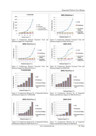
All the experimental results in Fig 13, 14, 15, and 16 are depicted to show the execution time of the four
algorithms at different support thresholds. It can be observed from these figures that, our Sequential Pattern Tree
mining approach performs much better than apriori based GSP algorithm and also outperforms PrefixSpan and
Tree Based Mining which are pattern growth approaches. This is also to be mentioned that, our proposed
approach generates same number of sequential patterns for different minimum support thresholds as generated by
GSP, PrefixSpan, and Tree Based Mining algorithms shown in Fig 17, 18, 19, and 20 respectively.
V. CONCLUSION
In this paper, we have proposed an efficient Sequential Pattern Tree Mining algorithm which can
generate the complete set of frequent sequential patterns from a Sequential Pattern Tree without generating any
candidate sequence and any intermediate projected tree that reduce the both space and time complexity. It does
not generate projected trees during mining by finding the first occurrence nodes from the suffix trees of prefix
subsequences. Also, it reduces the effort of repeated scanning of database due to storage of count in the tree‟s
node that help us to enhance the performance of our algorithm. This approach first generates a Sequential Pattern
Tree from the sequence database which stores both frequent and non-frequent items. So that, it requires only one
scan of sequence database to create the tree along with Header Table which also reduces the tree construction
time considerably. Again, our proposed approach reduces the usage of memory by storing only essential
information in the tree and by not generating projected trees during mining. Although we require little more
memory for storing non-frequent items in the tree, but in future we will be able to achieve better performance for
incremental mining because of these stored non-frequent items. We will show this in our future work. So that, we
can ignore this memory usage issue for the benefit of performance enhancement as memory is not so expensive at
the present time.

Figure 1: First Occurrence Node of „a‟ for “(a)"
Figure 2: First Occurrence Nodes of „a‟ for “(a)(a)"
Figure 3: First Occurrence Node of „a‟ for "(a)(a)(a)"
Figure 4: First Occurrence Node of „b‟ for "(a)(ab)"
Figure 5: First Occurrence Node of „a‟ for "(a)(ab)(a)"
Figure 6: Order to Generate Frequent Sequential Patterns

Figure 7: Comparisons Between Execution Time and
Minimum Support for T10I4D100K
Minimum Support for BMS-WebView-1
Minimum Support for BMS-WebView-2
Minimum Support for BMS-POS
Figure 11: Comparisons Between No. of Sequential Patterns
and Minimum Support for T10I4D100K
Figure 12: Comparisons Between No. of Sequential
Patterns and Minimum Support for BMS-WebView-1
Figure 19: Comparisons Between No. of Sequential Patterns
and Minimum Support for BMS-WebView-2
Figure 13: Comparisons Between No. of Sequential
Patterns and Minimum Support for BMS-POS

REFERENCES
[1] R. Agrawal and R. Srikant, “Mining sequential patterns," in ICDE, P. S. Yu and A. L. P. Chen, Eds. IEEE Computer Society, 1995,
pp. 3-14. [Online] Available: http://doi.ieeecomputersociety.org/10.1109/ICDE.1995.380415
[2] R. Srikant and R. Agrawal, “Mining sequential patterns: Generalizations and performance improvements," in EDBT, ser. Lecture
Notes in Computer Science, P. M. G. Apers, M. Bouzeghoub, and G. Gardarin, Eds., vol. 1057. Springer, 1996, pp. 3-17. [Online]
Available: http://dx.doi.org/10.1007/BFb0014140
[3] M. J. Zaki, “Spade: An efficient algorithm for mining frequent sequences," Machine Learning, vol. 42, no. 1/2, pp. 31-60, 2001.
[Online] Available: http://dx.doi.org/10.1023/A:1007652502315
[4] J. Han, J. Pei, B. Mortazavi-Asl, Q. Chen, U. Dayal, and M. Hsu, “Freespan: frequent pattern-projected sequential pattern mining,"
in KDD, 2000, pp. 355-359. [Online] Available: http://doi.acm.org/10.1145/347090.347167
[5] J. Pei, J. Han, B. Mortazavi-Asl, H. Pinto, Q. Chen, U. Dayal, and M. Hsu, “Prefixspan: Mining sequential patterns by prefix-
projected growth," in ICDE, D. Georgakopoulos and A. Buchmann, Eds. IEEE Computer Society, 2001, pp. 215-224. [Online]
Available: http://doi.ieeecomputersociety.org/10.1109/ICDE.2001.914830
[6] Bithi A. A., Akhter M., & Ferdaus A. A. “Tree Based Sequential Pattern Mining”, IRACST - International Journal of Computer
Science and Information Technology & Security (IJCSITS), ISSN: 2249-9555, Vol. 2, No.6, December 2012. [Online] Available:
http://www.ijcsits.org/papers/vol2no62012/25vol2no6.pdf
[7] C.-W. Lin, T.-P. Hong, W.-H. Lu, and W.-Y. Lin, “An incremental FUSP-tree maintenance algorithm," in ISDA, J.-S. Pan, A.
Abraham, and C.-C. Chang, Eds. IEEE Computer Society, 2008, pp. 445-449. [Online] Available:
http://doi.ieeecomputersociety.org/10.1109/ISDA.2008.126
[8] J. Han, J. Pei, and Y. Yin, “Mining frequent patterns without candidate generation," in SIGMOD Conference, W. Chen, J. F.
Naughton, and P. A. Bernstein, Eds. ACM, 2000, pp. 1-12. [Online] Available: http://doi.acm.org/10.1145/342009.335372
[9] J. Pei, J. Han, B. Mortazavi-asl, and H. Zhu, “Mining access patterns efficiently from web logs," 2000. [Online] Available:
http://citeseer.ist.psu.edu/264604.html;ftp://ftp.fas.sfu.ca/pub/cs/han/pdf/weblog00.pdf
[10] C. I. Ezeife and Y. Lu, “Mining web log sequential patterns with position coded pre-order linked WAP-tree," Data Min. Knowl.
Discov, vol. 10, no. 1, pp. 5-38, 2005. [Online] Available: http://dx.doi.org/10.1007/s10618-005-0248-3
[11] Z. Zheng, R. Kohavi, and L. Mason, “Real world performance of association rule algorithms," in KDD, 2001, pp. 401-406.
[Online] Available: http://portal.acm.org/citation.cfm?id=502512.502572

Sequential Pattern Tree Mining

More Related Content

What's hot

Viewers also liked

Similar to Sequential Pattern Tree Mining

More from IOSR Journals

Recently uploaded

Sequential Pattern Tree Mining