1760516799059_IF5141-1-2025-Module_05-Sequential-Pattern.pptx

1
PATTERN ADVANCED
MINING:
SEQUENTIAL PATTERN
Slides by:
Jiawei Han, Micheline Kamber, and Jian Pei
University of Illinois at Urbana-Champaign
Simon Fraser University
©2023 Han, Kamber, and Pei. All rights reserved.
The slides have been modified and rearranged by G.A. Putri Saptawati
for the purpose of course IF5141 Data Mining

2
Main
Source
Jianwei Han, Jian Pei, Hanghang Tong
“Data Mining: Concepts and Techniques”,
Fourth Edition, Elsevier Inc., 2023
 Chapter 5. Pattern Mining:
Advanced Methods

3
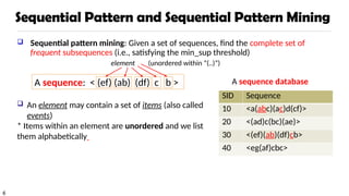
Sequential Pattern Mining
 Sequential Pattern and Sequential Pattern Mining
 GSP: Apriori-Based Sequential Pattern Mining
 SPADE: Sequential Pattern Mining in Vertical Data Format
 PrefixSpan: Sequential Pattern Mining by Pattern-Growth
 CloSpan: Mining Closed Sequential Patterns
 Constraint-Based Sequential-Pattern Mining

4
Sequential Pattern Mining
 What kind of patterns are sequential?
 Sequential: The order really matters
 You cannot swap two items in a sequence and have the same sequence
 Example: The English language is sequential: Subject → Verb → Object
 Other points:
 For Sequential Pattern Mining, the time which the items occur is not
considered
 Time Series Analysis does take into account the time in which an item
occurred

5
Sequential Pattern Examples
 Application of Sequential pattern Mining
 Customer shopping: Purchase a laptop first, then a digital camera, and then
a smartphone
 Medical treatments: Go to see a doctor, get drugs, doctor monitors
progress, doctor reacts accordingly → more/less drugs
 Natural disasters: Before the disaster, during the disaster, after the disaster
 Scientific Experiments: Step 1, Step 2, Step 3
 Stocks Markets: A set of stocks go up and down together
 Biological sequences, DNA /Protein: If you change the order of a protein, it
likely results in a different gene

6
Sequential Pattern and Sequential Pattern Mining
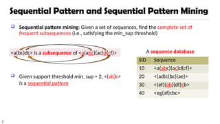
 Sequential pattern mining: Given a set of sequences, find the complete set of
frequent subsequences (i.e., satisfying the min_sup threshold)
A sequence database
 An element may contain a set of items (also called
events)
* Items within an element are unordered and we list
them alphabetically
A sequence: < (ef) (ab) (df) c b >
SID Sequence
10 <a(abc)(ac)d(cf)>
20 <(ad)c(bc)(ae)>
30 <(ef)(ab)(df)cb>
40 <eg(af)cbc>
element (unordered within “(..)”)

7
Sequential Pattern and Sequential Pattern Mining
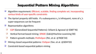
 Sequential pattern mining: Given a set of sequences, find the complete set of
frequent subsequences (i.e., satisfying the min_sup threshold)
<a(bc)dc> is a subsequence of <a(abc)(ac)d(cf)>
 Given support threshold min_sup = 2, <(ab)c>
is a sequential pattern
SID Sequence
20 <(ad)c(bc)(ae)>
30 <(ef)(ab)(df)cb>
40 <eg(af)cbc>
A sequence database

8
Sequential Pattern Mining Algorithms
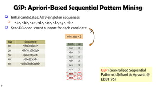
 Algorithm requirement: Efficient, scalable, finding complete set, incorporating
various kinds of user-specific constraints
 The Apriori property still holds: If a subsequence s1 is infrequent, none of s1’s
super-sequences can be frequent
 Representative algorithms
 GSP (Generalized Sequential Patterns): Srikant & Agrawal @ EDBT’96)
 Vertical format-based mining: SPADE (Zaki@Machine Leanining’00)
 Pattern-growth methods: PrefixSpan (Pei, et al. @TKDE’04)
 Mining closed sequential patterns: CloSpan (Yan, et al. @SDM’03)
 Constraint-based sequential pattern mining

9
GSP: Apriori-Based Sequential Pattern Mining
 Initial candidates: All 8-singleton sequences
 <a>, , <c>, <d>, <e>, <f>, <g>, <h>
 Scan DB once, count support for each candidate
SID Sequence
10 <(bd)cb(ac)>
20 <(bf)(ce)b(fg)>
30 <(ah)(bf)abf>
40 <(be)(ce)d>
50 <a(bd)bcb(ade)>
min_sup = 2
Cand. sup
<a> 3
 5
<c> 4
<d> 3
<e> 3
<f> 2
<g> 1
<h> 1
x
GSP (Generalized Sequential
Patterns): Srikant & Agrawal @
EDBT’96)

10
GSP: Apriori-Based Sequential Pattern Mining
 Example: Generate length-2 candidate sequences
min_sup = 2
Cand. sup
<a> 3
 5
<c> 4
<d> 3
<e> 3
<f> 2
<g> 1
<h> 1
<a> <c> <d> <e> <f>
<a> <aa> <ab> <ac> <ad> <ae> <af>
 <ba> <bb> <bc> <bd> <be> <bf>
<c> <ca> <cb> <cc> <cd> <ce> <cf>
<d> <da> <db> <dc> <dd> <de> <df>
<e> <ea> <eb> <ec> <ed> <ee> <ef>
<f> <fa> <fb> <fc> <fd> <fe> <ff>
<a> <c> <d> <e> <f>
<a> <(ab)> <(ac)> <(ad)> <(ae)> <(af)>
 <(bc)> <(bd)> <(be)> <(bf)>
<c> <(cd)> <(ce)> <(cf)>
<d> <(de)> <(df)>
<e> <(ef)>
<f>
 w/o pruning
(includes g and h):
8*8 + 8*7/2 = 92
length-2 candidates
 w/ pruning:
6*6 + 6*5/2 = 51
length-2 candidates
singleton * singleton – Total: (6 * 6)
Sets (unordered) – Total: (6*5) / 2
Apriori Pruning

11
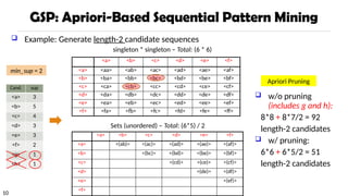
GSP Mining and Pruning
<a> <c> <d> <e> <f> <g> <h>
<aa> <ab> … <af> <ba> <bb> … <ff> <(ab)> … <(ef)>
<abb> <aab> <aba> <baa> <bab> …
<abba> <(bd)bc> …
<(bd)cba>
1st
scan: 8 cand. 6 length-1 seq. pat.
2nd
10 cand. not in DB at all
3rd
scan: 46 cand. 20 length-3 seq. pat. 20
cand. not in DB at all
4th
5th
SID Sequence
10 <(bd)cb(ac)>
20 <(bf)(ce)b(fg)>
30 <(ah)(bf)abf>
40 <(be)(ce)d>
50 <a(bd)bcb(ade)>
min_sup = 2
 Remove Candidates not in DB
or Candidates < min_sup
6*6 + 6*5/2 = 51
length
5
4
3
2
1
 Repeat, starting at k = 1 until k <= length
 Scan DB to find “length-k” frequent sequences
 Generate “length-(k+1)” candidate sequences from “length-k”
frequent sequences using Apriori
 set k = k+1
 Until no frequent sequence or no candidate can be found
The GPS algorithm

12
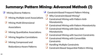
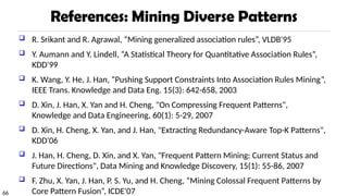
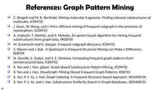
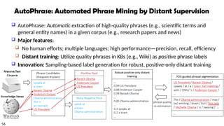
Sequential Pattern Mining in Vertical Data
Format: The SPADE Algorithm
SID Sequence
1 <a(abc)(ac)d(cf)>
2 <(ad)c(bc)(ae)>
3 <(ef)(ab)(df)cb>
4 <eg(af)cbc>
Ref: SPADE (Sequential
PAttern Discovery using
Equivalent Class) [M.
Zaki 2001]
min_sup = 2
 A sequence database is mapped to: <SID, EID>
 Grow the subsequences (patterns) one item at a time by Apriori candidate generation
EID (b) < EID (a):
Corresponds to:
<a(abc)(ac)d(cf)>

13
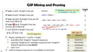
PrefixSpan: A Pattern-Growth Approach
 PrefixSpan Mining: Prefix Projections
 Step 1: Find length-1 sequential patterns
 <a>, , <c>, <d>, <e>, <f>
 Step 2: Divide search space and mine each projected DB
 <a>-projected DB,
 -projected DB,
 …
 <f>-projected DB, …
SID Sequence
20 <(ad)c(bc)(ae)>
30 <(ef)(ab)(df)cb>
40 <eg(af)cbc>
Prefix Suffix (Projection)
<a> <(abc)(ac)d(cf)>
<aa> <(_bc)(ac)d(cf)>
<ab> <(_c)(ac)d(cf)>
 Prefix and suffix
 Given <a(abc)(ac)d(cf)>
 Prefixes: <a>, <aa>,
<a(ab)>, <a(abc)>, …
 Suffix: Prefixes-based
projection
PrefixSpan (Prefix-projected
Sequential pattern mining)
Pei, et al. @TKDE’04
min_sup = 2
“_” is placeholder for prefix

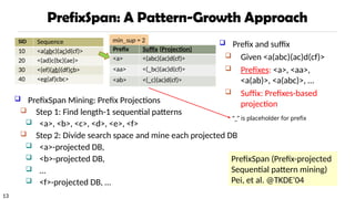
14
prefix <a>
PrefixSpan: Mining Prefix-Projected DBs
Length-1 sequential patterns
<a>, , <c>, <d>, <e>, <f>
prefix <aa>
…
prefix <af>
…
prefix 
prefix <c>, …, <f>
… …
SID Sequence
20 <(ad)c(bc)(ae)>
30 <(ef)(ab)(df)cb>
40 <eg(af)cbc>
<a>-projected DB
<(abc)(ac)d(cf)>
<(_d)c(bc)(ae)>
<(_b)(df)cb>
<(_f)cbc>
<aa>-projected DB <af>-projected DB
Major strength of PrefixSpan:
 No candidate subseqs. to be generated
 Projected DBs keep shrinking
min_sup = 2
-projected DB
<(_c)(ac)d(cf)>
<(_c)(ae)>
<(df)cb>
<c>
Length-2 sequential
patterns
<aa>, <ab>, <(ab)>,
<ac>, <ad>, <af>

16
CloSpan: Mining Closed Sequential Patterns
 A closed sequential pattern s: There exists no superpattern s’ such that s’ ‫כ‬ s, and s’
and s have the same support
 Which ones are closed? <abc>: 20, <abcd>:20, <abcde>: 15
 Why directly mine closed sequential patterns?
 Reduce # of (redundant) patterns
 Attain the same expressive power
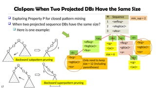
 Property P: Given two sequences s and s’, if s is a
subsequence of s’, then the projected database of s = the
projected database of s’ iff the size of the two projected
databases are the same.
 Explore Backward Subpattern and Backward
Superpattern pruning to prune redundant search space
 Greatly enhances efficiency (Yan, et al., SDM’03)

17
<efbcg>
<fegb(ac)>
<fea>
<e>
<a>
CloSpan: When Two Projected DBs Have the Same Size
<f>

ID Sequence
1 <aefbcg>
2 <afegb(ac)>
3 <afea>
<bcg>
<egb(ac)>
<ea>
<cg>
<(ac)>
<fbcg>
<gb(ac)>
<a>

<cg>
<(ac)>
<f>
<bcg>
<egb(ac)>
<ea>
 Exploring Property P for closed pattern mining
 When two projected sequence DBs have the same size?
 Here is one example:
Only need to keep
size = 12 (including
parentheses)
size = 6
Backward subpattern pruning
Backward superpattern pruning
min_sup = 2

56
 AutoPhrase: Automatic extraction of high-quality phrases (e.g., scientific terms and
general entity names) in a given corpus (e.g., research papers and news)
 Major features:
 No human efforts; multiple languages; high performance—precision, recall, efficiency
 Distant training: Utilize quality phrases in KBs (e.g., Wiki) as positive phrase labels
 Innovation: Sampling-based label generation for robust, positive-only distant training
AutoPhrase: Automated Phrase Mining by Distant Supervision

57
Robust Positive-Only Distant Training
 In each base classifier, randomly
sample K positive (e.g., wiki titles,
keywords, links) and K noisy
negative labels from the pools
 Noisy negative pool: may still have δ quality phrases among the K negative labels
 They form “perturbed training set”: size-2K subset of the full set of all phrases where
the labels of some quality phrases are switched from positive to negative
 Each base classifier can be viewed as randomly drawn K phrase candidates with
replacement from the positive pool and the negative pool respectively
 Grow an unpruned decision tree to the point of separating all phrases to meet this
requirement
 Use an ensemble classifier that averages the results of independently trained base
classifiers

58
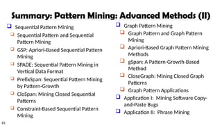
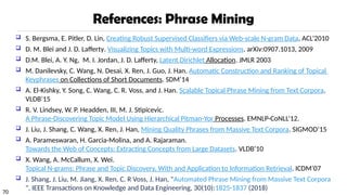
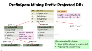
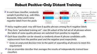
 Theoretical Analysis
 T base classifiers
 Exponentially decreasing
 Empirical Performance
 AUC to evaluate the ranking
Why Is Positive-Only Distant Training Robust?
Note: AUC (Area Under Curve), with value
range [0,1], is a classification measure to
be introduced in the classification module

59
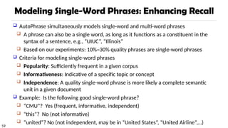
Modeling Single-Word Phrases: Enhancing Recall
 AutoPhrase simultaneously models single-word and multi-word phrases
 A phrase can also be a single word, as long as it functions as a constituent in the
syntax of a sentence, e.g., “UIUC”, “Illinois”
 Based on our experiments: 10%~30% quality phrases are single-word phrases
 Criteria for modeling single-word phrases
 Popularity: Sufficiently frequent in a given corpus
 Informativeness: Indicative of a specific topic or concept
 Independence: A quality single-word phrase is more likely a complete semantic
unit in a given document
 Example: Is the following good single-word phrase?
 “CMU”? Yes (frequent, informative, independent)
 “this”? No (not informative)
 “united”? No (not independent, may be in “United States”, “United Airline”,…)

60
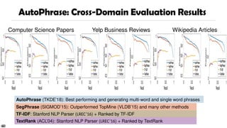
Computer Science Papers Yelp Business Reviews Wikipedia Articles
AutoPhrase: Cross-Domain Evaluation Results
60
SegPhrase (SIGMOD’15): Outperformed TopMine (VLDB’15) and many other methods
TF-IDF: Stanford NLP Parser (LREC’16) + Ranked by TF-IDF
TextRank (ACL’04): Stanford NLP Parser (LREC’16) + Ranked by TextRank
AutoPhrase (TKDE’18): Best performing and generating multi-word and single word phrases

61
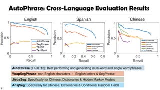
English Spanish Chinese
AutoPhrase: Cross-Language Evaluation Results
WrapSegPhrase: non-English characters  English letters & SegPhrase
JiebaSeg: Specifically for Chinese; Dictionaries & Hidden Markov Models
AnsjSeg: Specifically for Chinese; Dictionaries & Conditional Random Fields
AutoPhrase (TKDE’18): Best performing and generating multi-word and single word phrases

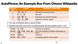
62
62
Phrase’s
Rank
Phrase Translation (Explanation)
1 江苏 _ 舜 _ 天 (the name of a soccer team)
2 苦 _ 艾 _ 酒 Absinthe
3 白发 _ 魔 _ 女 (the name of a novel/TV-series)
4 笔记 _ 型 _ 电脑 notebook computer, laptop
5 首席 _ 执行官 CEO
… … …
99,994 计算机 _ 科学技术 Computer Science and Technology
99,995 恒 _ 天然 Fonterra (a company)
99,996 中国 _ 作家 _ 协会 _ 副 _
主席
The Vice President of Writers Association of
China
99,997 维他命 _b Vitamin B
99,998 舆论 _ 导向 controlled guidance of the media
… … …
 The size of positive pool is about 29,000
 AutoPhrase finds more than 116,000 quality phrases (quality score > 0.5)
AutoPhrase: An Example Run From Chinese Wikipedia

63
Pattern Mining: Advanced Methods
 Mining Various Kinds of Patterns
 Mining Compressed or Approximate Patterns
 Constraint-based Pattern Mining
 Mining Sequential Patterns
 Mining Subgraph Patterns
 Pattern Mining: Application Examples
 Summary

64
Summary: Pattern Mining: Advanced Methods (I)
 Mining Diverse Patterns
 Mining Multiple-Level Associations
 Mining Multi-Dimensional
Associations
 Mining Quantitative Associations
 Mining Negative Correlations
 Mining Compressed and
Redundancy-Aware Patterns
 Constraint-Based Frequent Pattern Mining
 Why Constraint-Based Mining?
 Constrained Mining with Pattern Anti-
Monotonicity
 Constrained Mining with Pattern Monotonicity
 Constrained Mining with Data Anti-
Monotonicity
 Constrained Mining with Succinct Constraints
 Constrained Mining with Convertible
Constraints
 Handling Multiple Constraints
 Constraint-Based Sequential-Pattern Mining

65
Summary: Pattern Mining: Advanced Methods (II)
 Sequential Pattern Mining
 Sequential Pattern and Sequential
Pattern Mining
 GSP: Apriori-Based Sequential Pattern
Mining
 SPADE: Sequential Pattern Mining in
Vertical Data Format
 PrefixSpan: Sequential Pattern Mining
by Pattern-Growth
 CloSpan: Mining Closed Sequential
Patterns
 Constraint-Based Sequential Pattern
Mining
 Graph Pattern Mining
 Graph Pattern and Graph Pattern
Mining
 Apriori-Based Graph Pattern Mining
Methods
 gSpan: A Pattern-Growth-Based
Method
 CloseGraph: Mining Closed Graph
Patterns
 Graph Pattern Applications
 Application I: Mining Software Copy-
and-Paste Bugs
 Application II: Phrase Mining

66
References: Mining Diverse Patterns
 R. Srikant and R. Agrawal, “Mining generalized association rules”, VLDB'95
 Y. Aumann and Y. Lindell, “A Statistical Theory for Quantitative Association Rules”,
KDD'99
 K. Wang, Y. He, J. Han, “Pushing Support Constraints Into Association Rules Mining”,
IEEE Trans. Knowledge and Data Eng. 15(3): 642-658, 2003
 D. Xin, J. Han, X. Yan and H. Cheng, "On Compressing Frequent Patterns",
Knowledge and Data Engineering, 60(1): 5-29, 2007
 D. Xin, H. Cheng, X. Yan, and J. Han, "Extracting Redundancy-Aware Top-K Patterns",
KDD'06
 J. Han, H. Cheng, D. Xin, and X. Yan, "Frequent Pattern Mining: Current Status and
Future Directions", Data Mining and Knowledge Discovery, 15(1): 55-86, 2007
 F. Zhu, X. Yan, J. Han, P. S. Yu, and H. Cheng, “Mining Colossal Frequent Patterns by
Core Pattern Fusion”, ICDE'07

67
References: Constraint-Based Frequent Pattern Mining
 R. Srikant, Q. Vu, and R. Agrawal, “Mining association rules with item constraints”,
KDD'97
 R. Ng, L.V.S. Lakshmanan, J. Han & A. Pang, “Exploratory mining and pruning
optimizations of constrained association rules”, SIGMOD’98
 G. Grahne, L. Lakshmanan, and X. Wang, “Efficient mining of constrained correlated
sets”, ICDE'00
 J. Pei, J. Han, and L. V. S. Lakshmanan, “Mining Frequent Itemsets with Convertible
Constraints”, ICDE'01
 J. Pei, J. Han, and W. Wang, “Mining Sequential Patterns with Constraints in Large
Databases”, CIKM'02
 F. Bonchi, F. Giannotti, A. Mazzanti, and D. Pedreschi, “ExAnte: Anticipated Data
Reduction in Constrained Pattern Mining”, PKDD'03
 F. Zhu, X. Yan, J. Han, and P. S. Yu, “gPrune: A Constraint Pushing Framework for Graph
Pattern Mining”, PAKDD'07

68
References: Sequential Pattern Mining
 R. Srikant and R. Agrawal, “Mining sequential patterns: Generalizations and performance
improvements”, EDBT’96
 M. Zaki, “SPADE: An Efficient Algorithm for Mining Frequent Sequences”, Machine
Learning, 2001
 J. Pei, J. Han, B. Mortazavi-Asl, J. Wang, H. Pinto, Q. Chen, U. Dayal, and M.-C. Hsu,
"Mining Sequential Patterns by Pattern-Growth: The PrefixSpan Approach", IEEE TKDE,
16(10), 2004
 X. Yan, J. Han, and R. Afshar, “CloSpan: Mining Closed Sequential Patterns in Large
Datasets”, SDM'03
 J. Pei, J. Han, and W. Wang, "Constraint-based sequential pattern mining: the pattern-
growth methods", J. Int. Inf. Sys., 28(2), 2007
 M. N. Garofalakis, R. Rastogi, K. Shim: Mining Sequential Patterns with Regular Expression
Constraints. IEEE Trans. Knowl. Data Eng. 14(3), 2002
 H. Mannila, H. Toivonen, and A. I. Verkamo, “Discovery of frequent episodes in event
sequences”, Data Mining and Knowledge Discovery, 1997

69
References: Graph Pattern Mining
 C. Borgelt and M. R. Berthold, Mining molecular fragments: Finding relevant substructures of
molecules, ICDM'02
 J. Huan, W. Wang, and J. Prins. Efficient mining of frequent subgraph in the presence of
isomorphism, ICDM'03
 A. Inokuchi, T. Washio, and H. Motoda. An apriori-based algorithm for mining frequent
substructures from graph data, PKDD'00
 M. Kuramochi and G. Karypis. Frequent subgraph discovery, ICDM'01
 S. Nijssen and J. Kok. A Quickstart in Frequent Structure Mining can Make a Difference.
KDD'04
 N. Vanetik, E. Gudes, and S. E. Shimony. Computing frequent graph patterns from
semistructured data, ICDM'02
 X. Yan and J. Han, gSpan: Graph-Based Substructure Pattern Mining, ICDM'02
 X. Yan and J. Han, CloseGraph: Mining Closed Frequent Graph Patterns, KDD'03
 X. Yan, P. S. Yu, J. Han, Graph Indexing: A Frequent Structure-based Approach, SIGMOD'04
 X. Yan, P. S. Yu, and J. Han, Substructure Similarity Search in Graph Databases, SIGMOD'05

70
References: Phrase Mining
 S. Bergsma, E. Pitler, D. Lin, Creating Robust Supervised Classifiers via Web-scale N-gram Data, ACL’2010
 D. M. Blei and J. D. Lafferty. Visualizing Topics with Multi-word Expressions. arXiv:0907.1013, 2009
 D.M. Blei, A. Y. Ng, M. I. Jordan, J. D. Lafferty, Latent Dirichlet Allocation. JMLR 2003
 M. Danilevsky, C. Wang, N. Desai, X. Ren, J. Guo, J. Han. Automatic Construction and Ranking of Topical
Keyphrases on Collections of Short Documents. SDM’14
 A. El-Kishky, Y. Song, C. Wang, C. R. Voss, and J. Han. Scalable Topical Phrase Mining from Text Corpora.
VLDB’15
 R. V. Lindsey, W. P. Headden, III, M. J. Stipicevic.
A Phrase-Discovering Topic Model Using Hierarchical Pitman-Yor Processes. EMNLP-CoNLL’12.
 J. Liu, J. Shang, C. Wang, X. Ren, J. Han, Mining Quality Phrases from Massive Text Corpora. SIGMOD’15
 A. Parameswaran, H. Garcia-Molina, and A. Rajaraman.
Towards the Web of Concepts: Extracting Concepts from Large Datasets. VLDB’10
 X. Wang, A. McCallum, X. Wei.
Topical N-grams: Phrase and Topic Discovery, With and Application to Information Retrieval. ICDM’07
 J. Shang, J. Liu, M. Jiang, X. Ren, C. R Voss, J. Han, "Automated Phrase Mining from Massive Text Corpora
", IEEE Transactions on Knowledge and Data Engineering, 30(10):1825-1837 (2018)

1760516799059_IF5141-1-2025-Module_05-Sequential-Pattern.pptx

More Related Content

Similar to 1760516799059_IF5141-1-2025-Module_05-Sequential-Pattern.pptx

Recently uploaded

1760516799059_IF5141-1-2025-Module_05-Sequential-Pattern.pptx

Editor's Notes