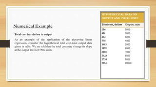
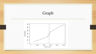
Piecewise Linear Regression

1. Piecewise Linear regression
(Segmented regression)

2. Motivation
 Traditional linear regression assumes a constant relationship between the
independent variable (X) and the dependent variable (Y). However, in
many real-world scenarios, this assumption might not hold across the
entire range of X.

3. Piecewise Linear regression
• Piecewise linear regression acknowledges that the relationship between X and Y may
change at specific points or thresholds. Instead of fitting a single linear model for the
entire dataset, we break the range of X into segments and allow for different linear
relationships within each segment.
• Piecewise linear regression finds application in environmental studies, economic analysis,
and policy impact assessment, especially where relationships exhibit non-linear patterns,
thresholds, or abrupt changes.

4. Graphical Representation

5. Figure Explanation
• It is assumed that sales commission increases linearly with sales until the
threshold level X*, after which also it increases linearly with sales but at a
much steeper rate. Thus, we have a piecewise linear regression consisting of
two linear pieces or segments, which are labeled I and II in Figure, and the
commission function changes its slope at the threshold value. Given the data
on commission, sales, and the value of the threshold level X*.

6. Statistical Model
The technique of dummy variables can be used to estimate the (differing) slopes of the two
segments of the piecewise linear regression. We proceed as follows:
𝑌𝑖 = β0 + β1𝑋𝑖 + β2(𝑋𝑖 – 𝑋∗
)*D + μ𝑖
where 𝑌𝑖 = sales commission
𝑋𝑖 = volume of sales generated by the sales person
𝑋∗
= threshold value of sales also known as a knot
D = 1 if 𝑋𝑖> 𝑋∗
= 0 if 𝑋𝑖 < 𝑋∗

7. Continued
Assuming E(μ𝑖
) = 0, we see at once that
E(Y𝑖 | D𝑖 = 0, X𝑖 , 𝑋∗
) = α𝑖 + β1
X𝑖
which gives the mean sales commission up to the target level 𝑋∗
and
E(Y𝑖 | D𝑖 = 1, X𝑖 , 𝑋∗
) = α𝑖 +β1𝑋𝑖 +β2 (𝑋𝑖 – 𝑋∗
) * (1)
E(Y𝑖 | D𝑖 = 1, X𝑖 , 𝑋∗
) = α𝑖 −β2
𝑋∗
+ (β1
+ β2
)X𝑖
which gives the mean sales commission beyond the target level 𝑋∗
.
β1
gives the slope of the regression line in segment I, and β1
+ β2
gives the
slope of the regression line in segment II of the piecewise linear regression
shown in Figure.

8. Real life Application
• Retail Sales - Consumer Spending Habits
In retail, the relationship between pricing strategies and consumer spending
might vary during different promotional periods. Piecewise linear regression
can help identify breakpoints where changes in consumer behavior, such as
increased responsiveness to discounts, occur.

9. Continued
• Economic Analysis - Impact of Tax Policies
In economic analysis, researchers may explore the impact of tax policies on
consumer spending. A dataset could exhibit different consumer behaviors
before and after the implementation of a tax policy change. Piecewise linear
regression could be employed to model the distinct relationships between
income and spending in each policy regime.

10. Continued
• Environmental Studies - Ecological Response to Temperature
Imagine scientists studying the population dynamics of a specific penguin
species in Antarctica. Penguins might thrive in relatively cooler temperatures,
where they have access to abundant food sources from the ocean. However, as
temperatures become extremely cold, it might impact their ability to find food,
leading to population declines.

11. Numerical Example
Total cost in relation to output
As an example of the application of the piecewise linear
regression, consider the hypothetical total cost-total output data
given in table. We are told that the total cost may change its slope
at the output level of 5500 units.

12. Graph

13. Solution
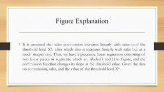
Y X1 X1 – X* D X2 = (X1 – X*)*D
256 1000 -4500 0 0
414 2000 -3500 0 0
634 3000 -2500 0 0
778 4000 -1500 0 0
1003 5000 -500 0 0
1839 6000 500 1 500
2081 7000 1500 1 1500
2423 8000 2500 1 2500
2734 9000 3500 1 3500
2914 10000 4500 1 4500
Let Y represent total cost and X total output, we
obtain the following results:
n = 10 , k = 3
Yi = β0 + β1X1 + β2(X1 – X*)*D + μi
𝛽1 =
𝑐𝑜𝑣 𝑋1,𝑌 𝑣𝑎𝑟 𝑋2 −𝑐𝑜𝑣 𝑋2,𝑌 𝑐𝑜𝑣 (𝑋1 ,𝑋2)
𝑣𝑎𝑟 𝑋1 𝑣𝑎𝑟 𝑋2 −[𝑐𝑜𝑣 (𝑋1 ,𝑋2)]2
𝛽1 =
2692600 2562500 −(1393550)(4125000)
8249999.866 2562500 −[4125000]2
𝛽1 = 0.2791

14. Continued…
𝛽2 =
𝑐𝑜𝑣 𝑋2,𝑌 𝑣𝑎𝑟 𝑋1 −𝑐𝑜𝑣 𝑋1,𝑌 𝑐𝑜𝑣 (𝑋1 ,𝑋2)
𝑣𝑎𝑟 𝑋1 𝑣𝑎𝑟 𝑋2 −[𝑐𝑜𝑣 (𝑋1 ,𝑋2)]2
𝛽2 =
1393550 8249999.866 −(2692600)(4125000)
8249999.866 2562500 − 41250002
𝛽2 = 0.0945
𝛽0 = 𝑌 − 𝛽1 𝑋1 − 𝛽2 𝑋2
𝛽0 = 1507.6 – (0.2791)(5500) – (0.0945)(1250)
𝛽0 = – 145.7167
Xi* = 5500
The estimated model is
𝑌i = – 145.7167 + 0.2791 Xi + 0.0945 (Xi – 5500) Di

15. Testing for β0
Hypothesis
H0: β0 = 0
H1: β0 ≠ 0
Level of significance
α = 0.05
Test statistic
t =
𝛽0
−
𝑆𝐸 (𝛽0
)
Computation
t =
− 145.7167−0
176.73415
t = −0.824
Critical region
𝑡𝑐𝑎𝑙 ≥ 𝑡𝛼
2
,𝑛−𝑘
= 1.895
Conclusion
Accept H0

16. Testing for β1
Hypothesis
H0: β1 = 0
H1: β1 ≠ 0
Level of significance
α = 0.05
Test statistic
t =
𝛽1
−
𝑆𝐸 (𝛽1
)
Computation
t =
0.2791− 0
0.04601
t = 6.066
Critical region
𝑡𝑐𝑎𝑙 ≥ 𝑡𝛼
2
,𝑛−𝑘
= 1.895
Conclusion
Reject H0

17. Testing for β2
Hypothesis
H0: β2 = 0
H1: β2 ≠ 0
Level of significance
α = 0.05
Test statistic
t =
𝛽2
−
𝑆𝐸 (𝛽2
)
Computation
t=
0.0945−0
0.08255
t = 1.144
Critical region
𝑡𝑐𝑎𝑙 ≥ 𝑡𝛼
2
,𝑛−𝑘
= 1.895
Conclusion
Accept H0

18. Conclusion
As,
𝑌i = – 145.7167 + 0.2791 Xi + 0.0945 (Xi – 5500) Di
H0: β2 = 0
Which gives a 𝑡𝑐𝑎𝑙 = 1.144 less than tabulated value 1.895 do not falls in critical
region , and P_value = 0.289950 greater than the level of significance 0.05. β2 is
not statistically significant because the dummy variable is not significant at 5
percent level. For practical purpose, one can regress total cost (Y) on total
output (X), dropping the dummy variable.

19. Comparison b/w SLR and Piecewise Linear Regression
Simple Linear Regression Piecewise Linear Regression

20. Example 2
X Y
100 9.73
120 9.61
140 8.15
160 6.98
180 5.87
200 4.98
220 5.09
240 4.79
260 4.02
280 4.46
300 3.82
An operations research analyst is investigating the
relationship between production lot size X and the average
production cost per unit Y . A study of recent operations
provides the data in table. The analyst suspects that a
piecewise linear regression model should be fit to this data.
Estimate the parameters in such a model assuming that the
slope of the line changes at 𝑋∗
= 200 units.

21. Graph

22. Solution
Y X1 X1–X* D
X2 = (X1 –
X*)*D
9.73 100 -100 0 0
9.61 120 -80 0 0
8.15 140 -60 0 0
6.98 160 -40 0 0
5.87 180 -20 0 0
4.98 200 0 0 0
5.09 220 20 1 20
4.79 240 40 1 40
4.02 260 60 1 60
4.46 280 80 1 80
3.82 300 100 1 100
Let Y represent average production cost per unit and X production
lot size, we obtain the following results in matrix form :
𝑌 = β * X+ μ𝑖
Where β = (𝑋′
𝑋)−1
𝑋′
Y
cov(β) = σ2
(𝑋′
𝑋)−1
β =
15.1164
−0.0501
0.0388
; n = 11 , k = 3 , 𝑋∗
= 200
𝑌= 15.1164 − 0.0501 𝑋𝑖 + 0.0388(𝑋𝑖 – 200)*D

23. Testing for β0
Hypothesis
H0: β0 = 0
H1: β0 ≠ 0
Level of significance
α = 0.05
Test statistic
t =
𝛽0
−
𝑆𝐸 (𝛽0
)
Computation
t =
15.1164−0
0.5353
t = 28.235
Critical region
𝑡𝑐𝑎𝑙 ≥ 𝑡𝛼
2
,𝑛−𝑘
= 2.306
Conclusion
Reject H0

24. Testing for β1
Hypothesis
H0: β1 = 0
H1: β1 ≠ 0
Level of significance
α = 0.05
Test statistic
t =
𝛽1
−
𝑆𝐸 (𝛽1
)
Computation
t =
−0.0501− 0
0.0033
t = -15.065
Critical region
𝑡𝑐𝑎𝑙 ≥ 𝑡𝛼
2
,𝑛−𝑘
= 2.306
Conclusion
Reject H0

25. Testing for β2
Hypothesis
H0: β2 = 0
H1: β2 ≠ 0
Level of significance
α = 0.05
Test statistic
t =
𝛽2
−
𝑆𝐸 (𝛽2
)
Computation
t=
0.03885−0
0.00594
t = 6.534
Critical region
𝑡𝑐𝑎𝑙 ≥ 𝑡𝛼
2
,𝑛−𝑘
= 2.306
Conclusion
Reject H0

26. Conclusion
Data do support suspect of analyst that a piecewise linear regression model should
be fit. As,
𝑌= 15.1164 − 0.0501 𝑋𝑖 + 0.0388(𝑋𝑖 – 200)*D
H0: β2 = 0
Which gives a 𝑡𝑐𝑎𝑙 = 6.53 greater than tabulated value 2.306 falls in critical region , and
P_value = 0.000181 less than the level of significance 0.05. β2 is statistically significant
at 5 percent level. For practical purpose, one can regress average production cost per
unit (Y) on production lot size (X) and the dummy variable (D).

27. Comparison b/w SLR and Piecewise Linear Regression
Simple Linear Regression Piecewise Linear Regression

28. References
• Montgomery, D. C., Peck, E. A., & Vining, G. G. (2021). Introduction to
linear regression analysis. John Wiley & Sons.
• Gujarati, D. N., & Porter, D. C. (2009). Basic econometrics.
McGraw-hill.
• Leenaerts, D., & Van Bokhoven, W. M. (2013). Piecewise linear modeling
and analysis. Springer Science & Business Media.