This document is the master's thesis of Miquel Perelló Nieto submitted to Aalto University. The thesis examines merging chrominance and luminance in early, medium, and late fusion using Convolutional Neural Networks (CNNs) for image classification. The thesis demonstrates that fusing luminance and chrominance channels can improve CNNs' ability to learn visual features and outperforms models that do not fuse the channels. The thesis contains background chapters on image classification, neuroscience, artificial neural networks, CNNs, and the history of connectionism. It then describes the author's experiments comparing CNN architectures that fuse luminance and chrominance channels at different stages to a basic CNN model.


![Mathematical Notation
• This thesis contains some basic mathematical notes.
• I followed notation from [Bishop, 2006]
– Vectors: lower case Bold Roman column vector w or w = (w1, . . . , wM )
– Vectors: row vector is the transpose wT
or wT
= (w1, . . . , wM )T
– Matrices: Upper case Bold Roman M
– Closed interval: [a, b]
– Open interval: (a, b)
– Semi-closed interval: (a, b] and [a, b)
– Unit/identity matrix: of ize M × M is IM
xiii](https://image.slidesharecdn.com/146c407b-3fa0-4973-a3fa-401852309d94-160905130833/85/mscthesis-13-320.jpg)


![6 CHAPTER 2. IMAGE CLASSIFICATION
Finally, we present some famous datasets that have been used from the 80’s to
the present day in Section 2.9.
A more complete and accurate description of the field of computer vision and
digital images can be found in the references [Szeliski, 2010] and [Glassner, 1995].
2.1 What is image classification?
Image classification consists of identifying which is the best description for a given
image. This task can be ambiguous, as the best description can be subjective de-
pending on the person. It could refer to the place where the picture was taken, the
emotions that can be perceived, the different objects, the identity of the object, or to
several other descriptions. For that reason, the task is usually restricted to a specific
set of answers in terms of labels or classes. This restriction alleviates the problem
and makes it tractable for computers; the same relaxation applies to humans that
need to give the ground truth of the images. As a summary, the image classification
problem consists of the classification of the given into one of the available options.
It can be difficult to imagine that identifying the objects or labeling the images
could be a difficult task. This is because people do not need to perform conscious
mental work in order to decide if one image contains one specific object or not; or
if the image belongs to some specific class. We also see in other animals similar
abilities, many species are able to differentiate between a dangerous situation and
the next meal. But, one of the first insights into the real complexity occurred in
1966, when Marvin Minsky and one of his undergraduate students tried to create a
computer program able to describe what a camera was watching (See [Boden, 2006],
p. 781, originally from [Crevier, 1993]). On that moment, the professor and the
student did not realize about the real complexity of the problem. Nowadays it is
known to be a very difficult problem, belonging to the class of inverse problems, as
we try to classify 2D projections from a 3D physical world.
The difficulty of this task can be easier to understand if we examine the image
represented in a computer. Figure 2.1 shows three examples from the CIFAR-10
dataset. From the first two columns it is easy to identify to which classes the
images could belong. That is because our brain is able to identify the situation of
the main object, to draw the boundaries between objects, to identify their internal
parts, and to classify the object. The second column contains the same image
in gray-scale. In the last column the gray value of the images has been scaled
from the range [0, 255] to [0, 9] (this rescaling is useful for visualization purposes).
This visualization is a simplified version of the image that a computer sees. This
representation can give us an intuition about the complexity for a computer to
interpret a batch of numbers and separate the object from the background. For a
more detailed theoretical explanation about the complexity of object recognition see
the article [Pinto et al., 2008].
In the next steps, we see an intuitive plan to solve this problem.
1. Because the whole image is not important to identify the object, we first need
to find the points that contain interesting information. Later, this collection](https://image.slidesharecdn.com/146c407b-3fa0-4973-a3fa-401852309d94-160905130833/85/mscthesis-30-320.jpg)
![2.1. WHAT IS IMAGE CLASSIFICATION? 7
0 5 10 15 20 25 30
0
5
10
15
20
25
30
0 5 10 15 20 25 30
0
5
10
15
20
25
30
0 5 10 15 20 25 30
0
5
10
15
20
25
30
6
6
6
6
6
6
6
7
6
6
6
4
3
4
4
3
3
3
3
3
3
3
3
3
2
2
2
2
2
2
2
2
6
6
6
6
7
6
7
7
7
6
5
4
4
4
4
4
4
3
3
3
3
3
3
2
2
3
2
2
2
3
2
2
6
6
6
7
7
7
7
7
7
6
5
4
5
4
4
4
4
4
3
3
3
3
3
3
3
3
3
3
2
3
2
2
6
7
7
7
7
7
7
7
7
6
5
4
4
4
4
4
4
4
3
3
3
3
3
3
3
3
3
3
3
3
3
3
6
7
7
7
7
7
7
7
7
6
4
3
4
4
4
4
4
4
3
3
3
3
3
3
3
3
3
3
3
3
3
3
6
7
7
7
7
7
7
7
7
7
6
4
4
5
4
4
3
4
4
4
4
5
5
5
5
4
4
3
3
3
3
3
6
7
7
7
7
7
6
5
4
5
7
7
7
6
5
5
5
7
7
7
6
6
6
6
5
4
5
4
3
3
3
3
7
7
7
7
7
6
2
1
0
1
7
7
8
8
8
8
8
8
7
4
3
3
3
2
1
1
3
4
4
4
3
3
7
7
7
7
6
2
1
1
1
2
3
2
3
4
7
7
6
5
4
4
3
3
1
0
1
3
3
4
4
4
4
3
7
7
7
7
4
1
1
1
1
1
0
0
0
1
2
2
3
5
7
7
6
5
3
2
2
3
4
4
4
4
4
4
7
7
7
7
2
0
1
1
0
0
0
0
0
0
1
1
4
6
6
6
6
6
6
6
4
3
4
4
4
4
4
4
7
7
7
7
2
0
0
0
0
0
0
0
0
2
4
4
4
4
4
4
4
2
1
4
5
5
4
4
4
4
4
4
7
7
7
7
4
0
0
0
0
0
0
0
1
3
4
5
4
4
4
4
4
2
0
3
4
4
4
4
4
4
4
4
7
7
7
7
5
1
1
1
1
0
0
0
0
1
4
5
4
4
4
4
4
1
1
3
4
4
4
4
4
4
4
4
7
7
7
7
6
1
0
1
1
1
2
1
0
0
3
5
4
4
4
4
4
2
0
3
4
4
4
4
4
4
4
4
7
7
7
7
7
2
0
1
4
4
6
3
1
0
2
4
4
4
4
4
4
2
1
3
4
4
4
4
4
4
4
4
7
7
7
7
6
1
0
3
7
7
6
3
2
2
3
4
5
4
4
4
4
2
1
3
4
4
4
4
4
4
4
4
7
7
7
7
6
1
2
7
7
3
1
1
1
3
3
5
5
4
4
4
5
4
4
5
4
4
4
4
4
4
4
4
7
7
7
7
6
2
5
8
3
0
0
0
2
4
3
4
4
4
5
6
6
5
4
3
4
4
4
4
4
4
4
4
7
7
7
7
5
3
6
5
1
0
0
0
1
2
2
1
1
3
4
5
5
2
1
2
3
4
4
4
4
4
4
4
7
7
7
7
6
6
6
1
0
0
0
0
0
0
0
0
0
0
0
1
4
5
5
6
4
4
4
4
4
4
4
4
7
7
7
7
6
7
5
0
0
0
1
1
0
0
0
1
1
2
2
2
3
5
5
5
6
5
4
4
4
4
4
4
7
7
7
7
6
7
7
2
1
0
0
0
0
0
2
4
4
4
4
4
4
3
2
3
4
4
4
4
4
4
4
4
7
7
7
6
4
4
7
7
6
3
0
0
0
0
3
4
4
4
4
4
4
3
2
3
4
4
4
4
4
4
4
4
7
7
5
3
2
1
4
8
9
7
2
1
1
2
4
4
4
4
4
4
4
3
2
1
2
4
4
4
4
4
4
3
7
7
5
4
3
2
3
5
8
8
7
6
6
7
7
4
1
1
2
2
2
2
1
0
1
2
4
4
4
4
3
3
6
7
6
5
3
2
2
1
3
7
8
7
7
7
6
1
0
0
0
0
2
2
2
1
1
2
3
4
4
4
3
3
6
7
6
5
3
2
1
0
0
2
5
4
4
7
7
6
4
1
0
3
7
7
6
5
6
5
3
4
4
4
3
3
6
6
6
4
2
2
1
1
0
1
2
1
3
5
5
5
4
2
2
3
5
4
3
3
4
4
3
4
4
3
3
3
6
6
5
2
1
1
1
1
1
2
3
3
3
3
3
3
3
3
4
3
2
3
3
3
3
3
3
3
3
3
3
3
6
6
4
2
1
1
1
1
1
2
2
2
3
3
3
3
4
4
3
2
2
3
3
3
2
2
3
3
3
3
3
3
6
6
3
2
1
1
1
1
1
3
3
3
3
3
3
3
3
3
3
2
2
2
3
2
2
2
2
2
3
3
3
3
0 5 10 15 20 25 30
0
5
10
15
20
25
30
0 5 10 15 20 25 30
0
5
10
15
20
25
30
0 5 10 15 20 25 30
0
5
10
15
20
25
30
1
1
2
2
2
1
1
1
1
1
1
2
2
2
2
1
1
2
3
3
3
3
3
3
6
8
8
8
7
6
8
8
1
1
2
2
2
1
1
1
1
1
1
1
2
3
2
2
1
1
3
3
3
1
1
2
3
4
5
7
6
5
8
8
1
1
2
2
2
2
2
2
2
2
2
2
3
3
3
3
3
4
5
3
2
1
1
1
1
1
1
1
2
4
8
8
1
1
2
2
2
2
2
2
2
2
2
2
2
2
2
2
2
5
5
3
1
2
5
2
1
1
1
1
0
3
8
8
1
1
2
2
2
2
2
2
2
2
2
2
2
2
2
3
3
5
5
3
2
2
6
3
1
2
1
1
0
3
8
8
1
2
2
2
2
1
1
1
1
1
1
1
1
2
3
2
3
5
5
2
1
1
3
2
1
2
1
1
1
3
7
8
1
1
2
2
2
1
1
1
1
1
1
1
1
2
3
2
3
5
5
3
1
1
1
1
1
2
1
2
5
4
7
8
1
1
2
2
2
1
1
1
1
1
1
1
1
2
2
3
4
6
5
3
2
2
2
2
1
1
1
2
5
4
8
8
1
2
2
3
3
2
3
2
2
2
2
3
2
3
3
3
3
5
5
3
2
2
2
2
2
1
1
2
5
3
7
8
1
2
2
2
2
2
2
2
2
2
2
2
2
2
3
3
3
4
4
4
4
4
3
2
2
2
2
3
5
3
7
8
2
2
2
1
2
2
2
2
2
2
2
2
2
2
2
3
4
3
3
3
3
3
3
3
2
2
2
2
3
2
7
8
3
3
3
2
3
3
4
4
4
4
4
4
4
4
4
4
4
4
4
4
3
3
3
3
2
2
2
1
1
2
7
9
3
3
3
2
3
3
3
3
3
3
3
3
3
3
3
4
4
4
5
5
3
2
3
5
5
4
5
4
3
2
7
8
2
2
2
1
1
1
1
1
1
1
2
2
1
2
2
2
3
3
5
6
3
1
3
4
5
6
5
5
5
4
7
8
1
1
1
1
1
0
0
0
0
0
1
0
0
0
1
1
4
3
3
4
3
1
2
4
4
5
5
5
5
4
7
8
1
1
1
1
1
0
0
0
0
0
0
0
0
1
1
2
4
2
2
3
2
1
1
1
2
2
3
3
4
3
8
8
1
1
1
1
1
0
0
0
0
0
0
0
1
1
1
2
4
2
3
5
2
2
1
1
1
2
3
3
4
3
8
8
1
1
1
1
1
0
0
0
0
0
0
0
0
0
0
2
4
3
3
4
2
2
1
1
1
2
4
3
4
3
8
8
1
1
1
1
1
0
0
0
0
0
0
0
0
0
0
1
5
3
2
4
2
2
1
1
2
2
5
3
3
3
8
8
1
1
1
1
1
0
0
0
0
0
0
0
0
0
0
1
5
4
2
4
2
2
1
1
2
2
5
3
1
3
8
8
1
1
1
1
1
0
0
0
0
0
0
0
0
0
0
0
3
4
2
4
2
2
1
1
2
2
3
3
1
3
8
8
1
1
1
1
1
0
0
0
0
0
0
0
0
0
0
0
1
4
3
4
2
2
1
1
2
2
2
3
3
3
8
8
1
1
1
1
1
1
0
0
0
0
0
1
1
1
1
1
1
2
4
4
2
1
1
1
2
2
2
3
4
4
8
8
1
1
1
1
1
1
0
0
0
0
0
1
1
1
1
1
1
1
3
3
2
2
1
1
1
2
2
3
5
4
8
8
1
1
1
1
1
1
1
1
1
1
1
1
1
1
1
1
1
1
2
3
2
2
1
1
2
2
2
3
5
4
8
8
1
1
1
1
1
1
1
1
1
1
1
1
1
1
1
1
1
1
1
3
2
2
1
1
2
2
2
3
6
5
8
8
1
1
1
1
1
1
0
1
0
0
0
0
1
1
1
1
1
1
1
3
3
1
1
1
2
2
2
3
5
5
8
8
1
1
1
1
1
0
0
0
0
0
0
1
1
1
1
1
1
0
0
3
3
2
2
2
2
2
2
2
2
4
8
8
0
0
1
1
0
0
0
0
0
0
0
1
1
1
1
1
0
0
0
2
4
2
3
3
4
3
3
3
2
4
8
8
2
2
2
2
2
2
2
2
2
2
2
2
2
2
2
2
2
2
2
3
4
1
2
4
5
5
5
5
4
5
8
8
5
5
5
5
5
5
5
5
5
5
5
5
5
5
5
5
5
5
5
4
4
1
1
3
5
5
5
5
5
7
8
8
5
5
5
5
5
5
5
5
5
5
5
5
5
5
5
5
5
5
5
5
5
3
2
2
2
3
3
6
7
8
8
8
0 5 10 15 20 25 30
0
5
10
15
20
25
30
0 5 10 15 20 25 30
0
5
10
15
20
25
30
0 5 10 15 20 25 30
0
5
10
15
20
25
30
2
2
3
2
2
3
2
2
3
2
3
3
3
3
3
3
3
4
4
4
4
4
4
4
4
4
4
4
3
2
2
3
2
2
3
3
2
3
2
2
2
2
3
3
3
3
3
3
4
4
4
4
4
4
4
6
5
3
3
3
2
2
2
3
2
2
3
3
2
3
2
2
3
3
3
3
4
4
4
4
4
4
4
4
4
4
7
8
6
3
1
1
1
1
2
3
2
2
3
3
3
3
2
2
3
3
4
4
4
4
4
4
4
4
4
4
4
6
8
8
6
3
1
0
0
1
2
4
3
2
3
3
3
3
3
3
3
3
4
4
4
4
4
4
4
4
4
4
5
7
9
8
6
2
1
0
0
1
2
4
2
2
3
3
3
3
3
3
4
4
4
4
4
4
4
4
4
4
4
4
6
7
7
7
6
2
0
0
0
1
3
4
3
3
3
3
3
3
4
4
4
4
4
4
4
4
4
4
4
4
4
4
7
8
8
8
6
2
0
0
0
1
3
4
3
3
3
3
4
4
4
4
4
4
4
4
4
4
4
4
4
4
4
5
8
8
8
8
5
1
0
0
1
2
4
4
3
3
3
4
4
4
4
4
4
4
4
4
4
4
4
4
4
4
4
6
7
7
8
8
4
1
0
0
1
3
4
4
3
3
3
4
4
4
4
4
4
4
4
4
4
4
4
4
4
4
6
7
7
7
8
7
3
1
0
1
2
4
4
4
3
3
4
4
4
4
4
4
4
4
4
4
4
4
4
4
4
4
6
7
8
8
8
6
2
0
0
1
3
4
4
4
3
4
4
4
4
4
4
4
4
4
4
4
4
4
4
4
4
4
6
8
7
8
8
4
1
0
1
2
4
4
4
4
3
4
4
4
4
4
4
4
4
4
4
4
4
4
4
4
4
4
6
7
7
8
7
2
1
0
1
3
4
4
4
4
3
4
4
4
4
4
4
4
4
4
4
4
4
4
4
4
4
4
5
5
7
8
5
1
1
1
2
4
4
4
4
4
4
4
4
4
4
4
4
4
4
4
4
4
5
4
4
4
4
3
5
7
8
7
3
1
1
1
3
4
4
4
4
4
4
4
4
4
4
4
4
4
4
4
5
5
5
4
4
4
4
3
4
6
8
5
2
1
1
3
4
4
4
5
5
4
4
4
4
4
4
4
4
4
4
4
6
7
6
5
5
5
5
4
4
4
6
3
1
1
2
4
4
4
5
5
5
5
4
4
4
4
4
4
4
4
4
5
5
7
8
7
6
5
5
5
5
6
4
1
1
2
3
4
4
5
5
5
5
5
4
4
4
4
4
4
4
4
4
5
6
8
8
7
7
7
7
7
8
6
2
1
1
3
4
5
5
5
5
5
5
5
4
4
4
4
4
4
4
4
4
4
5
7
7
7
7
8
8
8
7
3
1
1
2
4
5
5
5
5
5
5
5
5
4
4
4
4
4
3
2
2
2
2
3
5
7
8
8
8
8
8
4
1
1
2
3
4
5
5
5
5
5
5
5
5
4
4
4
4
4
3
2
1
3
3
4
6
7
8
8
8
8
6
2
1
1
3
4
5
5
5
5
5
5
5
5
5
4
4
4
4
4
4
3
2
2
3
3
3
5
8
8
8
7
3
1
1
2
4
5
5
5
5
5
5
5
5
5
5
4
4
4
4
4
4
4
4
4
4
5
6
6
7
8
8
5
2
1
2
3
4
5
5
5
5
5
5
5
5
5
5
4
4
4
4
4
4
4
4
4
4
6
7
7
8
8
6
2
1
1
3
4
5
5
5
5
5
5
5
5
5
5
5
4
4
4
4
4
4
4
4
4
4
5
6
7
8
7
4
1
1
2
4
4
5
5
5
5
5
5
5
4
4
5
5
4
4
3
3
3
3
3
3
4
5
6
5
5
6
4
1
1
2
3
4
4
5
5
5
5
5
5
5
4
4
5
5
4
4
4
3
3
3
4
4
5
7
6
4
5
5
2
1
1
3
4
4
4
5
5
5
5
5
5
5
4
4
5
5
4
4
4
3
3
3
3
4
5
5
5
4
5
3
1
1
2
4
4
4
5
5
5
5
5
5
5
5
4
4
5
5
4
4
4
4
4
4
4
4
5
5
6
6
4
1
1
2
4
4
4
4
5
5
5
5
5
5
5
5
4
4
5
5
4
4
4
4
4
4
4
4
4
5
6
5
2
1
2
4
4
4
4
5
5
5
5
5
5
5
5
5
3
4
5
5
3
4
4
4
4
4
4
4
4
5
5
4
3
3
4
4
4
4
4
5
5
5
5
5
5
5
5
5
4
4
5
5
Figure 2.1: Digital image representation with some examples from the CIFAR-10
dataset.The first column contains the original images, second column the gray-scale,
and the last column contains the gray-scale values scaled to the range [0, 9]
of points can be used to define – for example – the object boundaries.
2. Group all the different collections of points to generate small objects or parts
that can explain larger – or more complex – objects.
3. In some cases identifying the background can be a very good prior in order to
classify the object. For example, if we are classifying animals and the picture is
taken under the sea, then it is more probable to find a sea lion than a savanna
lion.
4. All the extracted information conforms a set of features that we can use to
compare with past experiences and use these experiences to classify the new
images.
If the features that we are using are good enough and our past experiences cover
a large part of the possible situations it should be easy to decide which is the correct
class of the object. However, each of the previous steps has its own complexities
and researchers work on individual parts to find better solutions. Additionally, this
is a simplification of the common approach used in computer vision.
Although we saw a visual representation of the image stored in a computer, from
the mathematical point of view it is easier to imagine the three channels of the image](https://image.slidesharecdn.com/146c407b-3fa0-4973-a3fa-401852309d94-160905130833/85/mscthesis-31-320.jpg)

![2.2. IMAGE TRANSFORMATIONS 9
other transformations that can be applied to the images are explained in Section
2.2.
Once the limitations of the task are specified, it is possible to choose the features
that can be used. Usually, these features are based on the detection of edges, regions
and blobs throughout the image. These detectors are usually hand-crafted to find
such features that could be useful at the later stages. Some region detectors are
explained in Section 2.3, whilst some feature descriptors are shown in Section 2.4.
Then, given the feature descriptors it is possible to apply data mining and ma-
chine learning techniques to represent their distributions and find clusters of descrip-
tors that are good representatives of the different categories that we want to classify.
In Section 2.5 we give an introduction to some feature cluster representations.
Finally, with the clusters or other representations we can train a classification
model. This is often a linear Support Vector Machine (SVM), an SVM with some
kernel or a random forest.
2.1.2 Connectionism approach
Another approach is to use an Artificial Neural Network (ANN) to find automati-
cally the interesting regions, the feature descriptors, the clustering and the classifi-
cation. In this case the problem is on which structure of ANN to choose, and lots
of hyperparameters that need to be tuned and decided.
Convolutional Neural Network (CNN) have demonstrated to achieve very good
results on hand-written digit recognition, image classification, detection and local-
ization. For example, before 2012, the state-of-the-art approaches for image classifi-
cation were the previously mentioned and explained in the next sections. However,
in 2012, a deep CNN [Krizhevsky et al., 2012] won the classification task on Im-
ageNet Large Scale Visual Recognition Challenge (ILSVRC)2012. From that mo-
ment, the computer vision community started to became interested in the hidden
representation that these models were able to extract, and started using them as
a feature extractiors and descriptors. Figure 2.3 shows the number of participants
using CNNs during the period (2010-2014) in the ILSVRC image classification and
location challenges, together with the test errors of the winners in each challenge.
2.2 Image transformations
We explained previously that image classification belongs to the class of inverse
problems because the classification uses a projection of the original space to a lower
dimensional one; in this case from 3D to 2D. To solve this problem one of the
approaches consists in extracting features that are invariant to scale, rotation, or
perspective. However, these techniques are not always applied, because in some
cases, the restrictions of the problem in hand do not allow specific transformations.
Moreover, the use of these techniques reduces the initial information, possibly de-
teriorating the performance of the classification algorithm. For this reason, prior
knowledge of the task – or cross-validation – is very useful to decide which features](https://image.slidesharecdn.com/146c407b-3fa0-4973-a3fa-401852309d94-160905130833/85/mscthesis-33-320.jpg)

![2.3. REGION DETECTORS 11
(a) Harris-Laplace detector (b) Laplacian detector
Figure 2.4: Comparison of detected regions between Harris and Laplacian
detectors on two natural images (image from [Zhang and Marszalek, 2007])
positions. In general, the regions should be repeatable, invariant to illumination and
distinctive.
Edge detectors are a subclass of region detectors. They are focused on detect-
ing regions with sharp changes in brightness. The Canny detector [Canny, 1986]
is one of the most common edge detectors. Other options are the Sobel [Lyvers
and Mitchell, 1988], Prewitt [Prewitt, 1970] and Roberts cross operators. For an
extended overview about edge detectors see [Ziou and Tabbone, 1998].
The Harris corner detector [Harris and Stephens, 1988] is a more general region
detector. It describes one type of rotation-invariant feature detector based on a
filter of the type [−2, −1, 0, 1, 2]. Furthermore, the Laplacian detector [Lindeberg,
1998] is scale and affine-invariant and extracts blob-like regions (see Figure 2.4b).
Similarly, the Harris-Laplace detector [Mikolajczyk and Schmid, 2004; Mikolajczyk
et al., 2005a] detects also scale and affine-invariant regions. However, the detected
regions are more corner-like (see Figure 2.4a). Other common region detectors
include the Hessian-Laplace detector [Mikolajczyk et al., 2005b], the salient region
detector [Kadir and Brady, 2001], and Maximally Stable Extremal Region (MSER)
detector[Matas et al., 2004].
The blob regions, i.e. regions with variation in brightness surrounded by mostly
homogeneous levels of light, are often good descriptors. One very common blob
detector is the Laplacian of Gaussian (LoG) [Burt and Adelson, 1983]. In gray-scale
images where I(x, y) is the intensity of the pixel in the position [x, y] of the image
I, we can define the Laplacian as:
L(x, y) = ( 2
I)(x, y) =
∂2
I
∂x2
+
∂2
I
∂y2
(2.1)
Because of the use of the second derivative, small noise in the image is prone to
activate the function. For that reason, the image is smoothed with a Gaussian filter
as a pre-processing step. This can be done in one equation:
LoG(x, y) = −
1
πσ4
1 −
x2
+ y2
2σ2
e−x2+y2
2σ2
(2.2)](https://image.slidesharecdn.com/146c407b-3fa0-4973-a3fa-401852309d94-160905130833/85/mscthesis-35-320.jpg)
![12 CHAPTER 2. IMAGE CLASSIFICATION
10 5 0 5 10
0.10
0.05
0.00
0.05
0.10
0.15
0.20
G
dx G
dxdx G
(a) First and second derivative of
a Gaussian
x
6 4 2 0 2 4 6
y
6
4
2
0
2
4
6
0.000
0.005
0.010
0.015
0.020
0.025
0.030
0.035
0.040
(b) Gaussian G in 3D space
x
6 4 2 0 2 4 6
y
6
4
2
0
2
4
6
0.015
0.010
0.005
0.000
0.005
0.010
0.015
(c) ∂G
∂x
x
6 4 2 0 2 4 6
y
6
4
2
0
2
4
6
0.010
0.008
0.006
0.004
0.002
0.000
0.002
0.004
0.006
(d) ∂G
∂x2
x
6 4 2 0 2 4 6
y
6
4
2
0
2
4
6
0.010
0.008
0.006
0.004
0.002
0.000
0.002
0.004
0.006
(e) ∂G
∂y2
x
6 4 2 0 2 4 6
y
6
4
2
0
2
4
6
0.020
0.015
0.010
0.005
0.000
0.005
(f) LoG = ∂G
∂x2 + ∂G
∂y2
Figure 2.5: Laplacian of Gaussian
Also, the Difference of Gaussian (DoG) [Lowe, 2004] can find blob regions and
can be seen as an approximation of the LoG. In this case the filter is composed of the
subtraction of two Gaussians with different standard deviations. This approximation
is computationally cheaper than the former. Figure 2.6 shows a visual representation
of the DoG.
2.4 Feature descriptors
Given the regions of interest explained in the last section, it is possible to aggregate
them to create feature descriptors. There are several approaches to combine different
regions.
2.4.1 SIFT
Scale-Invariant Feature Transform (SIFT) [Lowe, 1999, 2004] is one of the most
extended feature descriptors. All previous region detectors were not scale invariant,
that is the detected features require a specific zoom level of the image. On the](https://image.slidesharecdn.com/146c407b-3fa0-4973-a3fa-401852309d94-160905130833/85/mscthesis-36-320.jpg)
![2.4. FEATURE DESCRIPTORS 13
0
0
Gσ1
Gσ2
DoG
(a) 1D
0
0
0
·10−2
(b) 2D
Figure 2.6: Example of DoG in one and two dimensions
contrary, SIFT is able to find features that are scale invariant – to some degree. The
algorithm is composed of four basic steps:
Detect extrema values at different scales
In the first step, the algorithm searches for blobs of different sizes. The objective
is to find Laplacian of Gaussian (LoG) regions in the image with different σ values,
representing different scales. The LoG detects the positions and scales in which the
function is strongly activated. However, computing the LoG is expensive and the
algorithm uses the Difference of Gaussian (DoG) approximation instead. In this
case, we have pairs of sigmas σl = kσl−1, where l represents the level or scale. An
easy approach to implement this step is to scale the image using different ratios,
and convolve different Gaussians with an increasing value of kσ. Then, the DoG is
computed by subtracting adjacent levels. In the original paper the image is rescaled
4 times and in each scale 5 Gaussians are computed with σ = 1.6 and k =
√
2 .
Once all the candidates are detected, they are compared with the 8 pixels that
are surrounding the point at the same level, as well as the 9 pixels in the upper and
lower levels. The pixel that has the largest activation is selected for the second step.
Refining and removing edges
Next, the algorithm performs a more accurate inspection of the previous candidates.
The inspection consists of computing the Taylor series expansion in the spatial
surrounding of the original pixel. In [Lowe, 1999] a threshold of 0.03 was selected
to remove the points that did not exceeded this value. Furthermore, because the
DoG is prone to detect also edges, a Harris corner detector is applied to remove
them. To find them, a 2 × 2 Hessian matrix is computed and the points in which
the eigenvalues are different with a certain degree are considered to be edges and
are discarded.](https://image.slidesharecdn.com/146c407b-3fa0-4973-a3fa-401852309d94-160905130833/85/mscthesis-37-320.jpg)
![14 CHAPTER 2. IMAGE CLASSIFICATION
Orientation invariant
The remaining keypoints are modified to make them rotation invariant. The sur-
rounding is divided into 36 bins covering the 360 degrees. Then the gradient in
each bin is computed, scaled with a Gaussian centered in the middle and with a σ
equal to 1.5 times the scale of the keypoint. Then, the bin with the largest value is
selected and the bins with a value larger than the 80% are also selected to compute
the final gradient and direction.
Keypoint descriptor
Finally, the whole area is divided into 16 × 16 = 256 small blocks. The small blocks
are grouped into 16 squared blocks of size 4 × 4. In each small block, the gradient
is computed and aggregated in eight circular bins covering the 360 degrees. This
makes a total of 128 feature descriptors that compose the final keypoint descrip-
tor. Additionally, some information can be stored to avoid possible problems with
brightness or other problematic situations.
2.4.2 Other descriptors
Speeded-Up Robust Features (SURF) [Bay et al., 2006, 2008] is another popular
feature descriptor. It is very similar to SIFT, but, it uses the integral of the original
image at different scales and finds the interesting points by applying Haar-like fea-
tures. This accelerates the process, but results in a smaller number of keypoints. In
the original paper, the authors claim that this reduced set of descriptors was more
robust than the ones discovered by SIFT.
Histogram of Oriented Gradients (HOG) [Dalal and Triggs, 2005] was originally
proposed for pedestrian detection and shares some ideas of SIFT. However, it is
computed extensively over the whole image, offering a full patch descriptor. Given
a patch of size 64 × 128 pixels, the algorithm divides the region into 128 small cells
of size 8 × 8 pixels. Then, the horizontal and vertical gradients at every pixel are
computed, and each 8 × 8 cell creates a histogram of gradients with 9 bins, divided
from 0 to 180 degrees (if the orientation of the gradient is important it can be
incorporated by computing the bins in the range 0 to 360 degrees). Then, all the
cells are grouped into blocks of 4×4 with 50% overlap with each adjacent block. This
makes a total of 7 × 15 = 105 blocks. Finally, the bins of each cell are concatenated
and normalized. This process creates a total of 105blocks × 4cells × 9bins = 3780features.
Other features are available but are not discussed here, some examples are the
Gradient location-orientation histogram (GLOH) [Mikolajczyk and Schmid, 2005]
with 17 locations, 16 orientation bins in a log-polar grid and uses Principal Com-
ponent Analysis (PCA) to reduce the dimensions to 128; the PCA-Scale-Invariant
Feature Transform (PCA-SIFT) [Ke and Sukthankar, 2004] that reduces the final
dimensions with PCA to 36 features; moment invariants [Gool et al., 1996]; SPIN
[Lazebnik et al., 2005]; RIFT [Lazebnik et al., 2005]; and HMAX [Riesenhuber and
Poggio, 1999].](https://image.slidesharecdn.com/146c407b-3fa0-4973-a3fa-401852309d94-160905130833/85/mscthesis-38-320.jpg)
![2.5. FEATURE CLUSTER REPRESENTATION 15
2.5 Feature Cluster Representation
All the previouslydiscussed detectors and descriptors can be used to create large
amounts of features to classify images. However, they result in very large feature
vectors that can be difficult to use for pattern classification tasks. To reduce the
dimensionality of these features or to generate better descriptors from the previous
ones it is possible to use techniques like dimensionality reduction, feature selection
or feature augmentation.
Bag of Visual words (BoV) [Csurka and Dance, 2004] was inspired by an older
approach for text categorization: the Bag of Words (BoW) [Aas and Eikvil, 1999].
This algorithm detects visually interesting descriptors from the images, and finds a
set of clusters representatives from the original visual descriptors. Then, the clusters
are used as reference points to form – later – a histogram of occurrences; each bin
of the histogram corresponds to one cluster. For a new image, the algorithm finds
the visual descriptors, computes their distances to the different clusters, and then
for each descriptor increases the count of the respective bin. Finally, the description
of the image is a histogram of occurrences where each bin is referred to as a visual
word.
Histogram of Pattern Sets (HoPS) [Voravuthikunchai, 2014] is a recent new al-
gorithm for feature representation. It is based on random selection of some of the
previously explained visual features (for example BoV). The selected features are
binarized: the features with more occurrences than a threshold are set to one, while
the rest are set to zero. The set of features with the value one creates a transac-
tion. The random selection and the creation of transactions is repeated P times
obtaining a total of P random transactions. Then, the algorithm uses data min-
ing techniques to select the most discriminative transactions, for example Frequent
Pattern (FP) [Agrawal et al., 1993] or Jumping Emerging Patterns (JEPs) [Dong
and Li, 1999]. Finally, the last representations is formed by 2 × P bins, two per
transaction: one for positive JEPs and the other for negative JEPs. In the original
paper this algorithm demonstrated state-of-the-art results on image classification
with the Oxford-Flowers dataset, object detection on PASCAL VOC 2007 dataset,
and pedestrian recognition.
2.6 Color
“We live in complete dark. What is color but
your unique interpretation of the electrical
impulses produced in the neuro-receptors of
your retina?”
— Miquel Perelló Nieto
The colors emerge from different electromagnetic wavelengths in the visible spec-
trum. This visible portion is a small range from 430 to 790 THz or 390 to 700nm
(see Figure 2.7). Each of these isolated frequencies creates one pure color, while
combinations of various wavelengths can be interpreted by our brain as additional](https://image.slidesharecdn.com/146c407b-3fa0-4973-a3fa-401852309d94-160905130833/85/mscthesis-39-320.jpg)


![2.9. DATASETS 21
subsample Y UV YUV factor
4:4:4 Iv × Ih 2 × Iv × Ih 3 × Iv × Ih 1
4:2:2 Iv × Ih 2 × Iv × Ih
2
2 × Iv × Ih 2/3
4:1:1 Iv × Ih 2 × Iv × Ih
4
3
2
× Iv × Ih 1/2
4:2:0 Iv × Ih 2 × Iv
2
× Ih
2
3
2
× Iv × Ih 1/2
Table 2.2: Chroma subsampling vertical, horizontal and final size reduction factor
summary of these transformations with the symbolic size of the different channels
of the YUV color space and the final size.
Figure 2.10 shows a visual example of the three subsampling methods previously
explained in the YUV color space, and how it would look if we apply the same
subsampling to the green and blue channels in the RGB color space. The same
amount of information is lost in both cases (in RGB and YUV), however, if only the
chrominance is reduced (YUV case) it is difficult to perceive the loss of information.
2.9 Datasets
In this section, we present a set of famous datasets that have been used from the
80s to evaluate different pattern recognition algorithms in computer vision.
In 1989, Yann LeCun created a small dataset of hand written digits to test
1989
the performance of backpropagation in Artificial Neural Networks (ANNs) [LeCun,
1989]. Later in [LeCun et al., 1989], the authors collected a large amount of samples
from the U.S. Postal Service and called it the MNIST dataset. This dataset is one
of the most widely used datasets to evaluate pattern recognition methods. The
test error has been dropped by state-of-the-art methods to 0%, but it is still being
used as a reference and to test semi-supervised or unsupervised methods where the
accuracy is not perfect.
The COIL Objects dataset [Nene et al., 1996] was one of the first image classifi-
cation datasets of a set of different objects. It was released in 1996. The objects were
1996
photographed in gray-scale, centered in the middle of the image and were rotated
by 5 degree steps throughout the full 360 degrees.
From 1993 to 1997, the Defense Advanced Research Projects Agency (DARPA)
collected a large number of face images to perform face recognition. The corpus was
1998
presented in 1998 with the name FERET faces [Phillips and Moon, 2000].
In 1999, researchers of the computer vision lab in California Institute of Technol-
1999
ogy collected pictures of cars, motorcycles, airplanes, faces, leaves and backgrounds
to create the first Caltech dataset. Later they released the Caltech-101 and Caltech-
256 datasets.
2001
In 2001, the Berkeley Segmentation Data Set (BSDS300) was released for group-
ing, contour detection, and segmentation of natural images [Martin and Fowlkes,
2001]. This dataset contains 200 and 100 images for training and testing with
12.000 hand-labeled segmentations. Later, in [Arbelaez and Maire, 2011], the au-](https://image.slidesharecdn.com/146c407b-3fa0-4973-a3fa-401852309d94-160905130833/85/mscthesis-45-320.jpg)

![2.9. DATASETS 23
thors extended the dataset with 300 and 200 images for training and test; in this
version the name of the dataset was modified to BSDS500.
In 2002, the Middleburry stereo dataset [Scharstein and Szeliski, 2002] was re-
2002
leased. This is a dataset of pairs of images taken from two different angles and with
the objective of pairing the couples.
In 2003, the Caltech-101 dataset [Fei-Fei et al., 2007] was released with 101
2003
categories distributed through 9.144 images of roughly 300 × 200 pixels. There are
from 31 to 900 images per category with a mean of 90 images.
In 2004, the KTH human action dataset was released. This was a set of 600
2004
videos with people performing different actions in front of a static background (a
field with grass or a white wall). The 25 subjects were recorded in 4 different
scenarios performing 6 actions: walking, jogging, running, boxing, hand waving and
hand clapping.
The same year, a collection of 1.050 training images of cars and non-cars was
released with the name UIUC Image Database for Car Detection. The dataset was
used in two experiments reported in [Agarwal et al., 2004; Agarwal and Roth, 2002].
In 2005, another set of videos was collected this time from surveillance cameras.
2005
The team of the CAVIAR project captured people walking alone, meeting with
another person, window shopping, entering and exiting shops, fighting, passing out
and leaving a package in a public place. The image resolution was of 384 × 288
pixels and 25 frames per second.
In 2006, the Caltech-256 dataset [Griffin et al., 2007] was released increasing the
2006
number of images to 30.608 and 256 categories. There are from 80 to 827 images
per category with a mean of 119 images.
In 2008, a dataset of videos of sign language [Athitsos et al., 2008] was released
2008
with the name American Sign Language Lexicon Video Dataset (ASLLVD). The
videos were captured from three angles: front, side and face region.
In 2009, one of the most known classification and detection datasets was released
2009
with the name of PASCAL Visual Object Classes (VOC) [Everingham and Gool,
2010; Everingham and Eslami, 2014]. Composed of 14.743 natural images of people,
animals (bird, cat, cow, dog, horse, sheep), vehicles (aeroplane, bicycle, boat, bus,
car, motorbike, train) and indoor objects (bottle, chair, dining table, potted plant,
sofa, tv/monitor). The dataset is divided into 50% for training and validation and
50% for testing.
In the same year, a team from Toronto University collected the CIFAR-10 dataset
(see Chapter 3 of [Krizhevsky and Hinton, 2009]). This dataset contained 60.000
color images of 32 × 32 pixel size divided uniformly between 10 classes (airplane,
automobile, bird, cat, deer, dog, frog, horse, ship and truck). Later, the number of
categories was increased to 100 in the extended version CIFAR-100.
ImageNet dataset was also released in 2009 [Deng et al., 2009]. This dataset
collected images containing nouns appearing in WordNet [Miller, 1995; Fellbaum,
1998] (a large lexical database of English). The initial dataset was composed by 5.247
synsets and 3.2 million images whilst in 2015 it was extended to 21.841 synsets and
2015
14.197.122 images.](https://image.slidesharecdn.com/146c407b-3fa0-4973-a3fa-401852309d94-160905130833/85/mscthesis-47-320.jpg)

![Chapter 3
Neuro vision
“He believes that he sees his retinal images: he
would have a shock if he could.”
— George Humphry
This Chapter gives a brief introduction about the neural anatomy of the visual
system. We hope that by understanding the biological visual system, it is possible to
get inspiration and design better algorithms for image classification. This approach
has been successfully used in the past in computer vision algorithms; for example,
the importance of blob-like features, or edge detectors. Additionally, some of the
state-of-the-art Artificial Neural Network (ANN) were originally inspired by the
cats and macaques visual system. We also know that humans are able to extract
very abstract representations of our environment by interpreting the different light
wavelengths that excite the photoreceptors in our retinas. As the neurons propagate
the electric impulses through the visual system our brain is able to create an abstract
representation of the environment [Fischler, 1987] (the so-called “signals-to-symbol”
paradigm).
Vision is one of the most important senses in human beings, as roughly the 60%
of our sensory inputs belong to visual stimulus. In order to study the brain we need
to study its morphology, physiology, electrical responses, and chemical reactions.
These characteristics are studied in different disciplines, however, they need to be
merged to solve the problem of understanding how the brain is able to create visual
representations of the surrounding. For that reason, the disciplines that are involved
in neuro vision extend from neurophysiology to psychology, chemistry, computer
science, physics and mathematics. In this chapter, first we introduce the biological
neuron, one of the most basic components of the brain in Section3.1. We give an
overview of the structure and the basics of their activations. Then, in Section 3.2,
we explain the different parts of the brain involved in the vision process, the cells,
and the visual information that they proceed. Finally, we present a summary about
the color perception, and the LMS color space in Section 3.3. For an extended
introduction to the human vision and how it is related to ANN see [Gupta and
Knopf, 1994].
25](https://image.slidesharecdn.com/146c407b-3fa0-4973-a3fa-401852309d94-160905130833/85/mscthesis-49-320.jpg)

![3.2. VISUAL SYSTEM 27
LMS r o d s
c o n e s
P a r v o c e l l u l a r
c e l l s
P r i m a r y
v i s u a l
c o r t e x
O p t i c c h i a s m a
O p t i c n e r v e
O p t i c a l l e n s
L a t e r a l
g e n i c u l a t e
n u c l e u s ( L G N )
E y e
N a s a l r e t i n a
Te m p o r a l
r e t i n a
Te m p o r a l
r e t i n a
L e f t v i s u a l
fi e l d
R i g h t v i s u a l
fi e l d
L i g h t
S i m p l e
C o m p l e x
H y p e r c o m p l e x
Figure 3.2: Visual pathway
3.2 Visual system
The visual system is formed by a huge number of nervous cells that send and receive
electrical impulses trough the visual pathway. The level of abstraction increases
as the signals are propagated from the retina to the different regions of the brain.
At the top level of abstraction there are the so-called “grandmother-cells” [Gross,
2002], these cells are specialized on detecting specific shapes, faces, or arbitrary
visual objects. In this section, we describe how the different wavelengths of light
are interpreted and transformed at different levels of the visual system. Starting
in the retina of the eyes in Section 3.2.1, going through the optic nerve, the optic
chiasma, and the Lateral Geniculate Nucleus (LGN) – allocated in the thalamus –
in Section 3.2.2, and finally the primary visual cortex in Section 3.2.3. Figure 3.2
shows a summary of the visual system and the connections from the retina to the
primary visual cortex. In addition, at the right side, we show a visual representation
of the color responses perceived at each level of the visual pathway.
3.2.1 The retina
The retina is a thin layer of tissue located in the inner and back part of the
eye. The light crosses the iris, the optical lens and the eye, and finally reaches the
photoreceptor cells. There are two types of photoreceptor cells: cone and rod cells.
Cone cells are cone shaped and are mostly activated with high levels of light.
There are three types of cone cells specialized on different wavelength: the short cells
are mostly activated at 420nm corresponding to a bluish color, the medium cells at](https://image.slidesharecdn.com/146c407b-3fa0-4973-a3fa-401852309d94-160905130833/85/mscthesis-51-320.jpg)
![28 CHAPTER 3. NEURO VISION
S y n a p t i c p e d i c l e
CR RCC
O p t i c
n e r v e
fi b e r
P h o t o r e c e p t o r s :
R o d s ( R ) a n d
C o n e s ( C )
B i p o l a r
c e l l s ( B )
H o r i z o n t a l
c e l l s ( H )
G a n g l i o n
c e l l s ( G )
G
A A
H
G G
B
B
L i g h t
s t i m u l u s
E y e
L i g h t
A m a c r i n e
c e l l s ( A )
Figure 3.3: A cross section of the retina with the different cells (the figure has
been adapted from [Gupta and Knopf, 1994]
400
Violet Blue Cyan Green Yellow Red
0
50
100
420
Short Rods Medium Long
534498 564
500
Wavelength (nm)
Normalizedabsorbance
600 700
(a) Human visual color response. The dashed line
is for the rod photoreceptor while red, blue, and
green are for the cones.
A n g u l a r s e p a r a t i o n f r o m t h e f o v e a
Ro d c e l l s
d e n s i t y
C o n e c e l l s
d e n s i t y
B l i n d
s p o t
Numberofcellspermm²
- 7 0 - 6 0 - 5 0 - 4 0 - 2 0- 3 0 - 1 0 0 º 7 06 05 04 02 0 3 01 0 8 0
2 0
4 0
6 0
8 0
1 2 0
1 0 0
1 4 0
1 8 0 0
1 6 0
0
x 1 0 ³
Fo v e a 0 º
( Te m p o r a l ) ( N a s a l )
(b) Rod and cone densities
Figure 3.4: Retina photoreceptors
534nm corresponding to a greenish color, and the long cells at 564nm corresponding
to a reddish color (see Figure 3.4a). These cells need large amounts of light to be
fully functional. For that reason, cone cells are used in daylight or bright conditions.
Their density distribution on the surface of the retina is almost limited to an area of
10 degrees around the fovea (see Figure 3.4b). For that reason, we can only perceive
color in a small area around our focus of attention – the perception of color in other
areas is created by more complex systems. There are about 6 million cone cells,
from which 64% are long cells, 32% medium cells and 2% short cells. Although the
number of short cells is one order of magnitude smaller than the rest, these cells
are more sensitive and being active in worst light conditions, additionally, there are
some other processes that compensate this difference. That could be a reason why
in dark conditions – when the cone cells are barely activated – the clearest regions
are perceived with a bluish tone.](https://image.slidesharecdn.com/146c407b-3fa0-4973-a3fa-401852309d94-160905130833/85/mscthesis-52-320.jpg)
![3.2. VISUAL SYSTEM 29
Rod cells do not perceive color but the intensity of light, their maximum re-
sponse corresponds to 498nm, between the blue and green wavelengths. They are
functional only on dark situations – usually during the night. They are very sensi-
tive, some studies (e.g. [Goldstein, 2013]) suggest that a rod cell is able to detect
an isolated photon. There are about 120 million of rod cells distributed trough all
the retina, while the central part of the fovea is exempt of them (see Figure 3.4b).
Additionally, the rod cells are very sensitive to motion and peripheral vision. There-
fore, in dim situations, it is easier to perceive movement and light in the periphery
but not in our focus of attention.
However, the photoreceptors are not connected directly to the brain. Their axons
are connected to the dendrites of other retinal cells. There are two types of cells
that connect the photoreceptors to other regions: the horizontal and bipolar cells.
Horizontal cells connect neighborhoods of cone and rod cells together. This
allows the communication between photoreceptors and bipolar cells. One of the most
important roles of horizontal cells, is to inhibit the activation of the photoreceptors
to adjust the vision to bright and dim light conditions. There are three types of
horizontal cells: HI, HII, and HIII; however their distinction is not clear.
Bipolar cells connect photoreceptors to ganglion cells. Additionally, they ac-
cept connections from horizontal cells. Bipolar cells are specialized on cones or rods.
There are nine types of bipolar cells specialized in cones, while only one type for
rod cells. Bipolar and horizontal cells work together to generate center surrounded
inhibitory filters with a similar shape of a Laplacian of Gaussian (LoG) or Difference
of Gaussian (DoG). These filters are focused in one color tone in the center and its
opposite at the bound.
Amacrine cells connect various ganglion and bipolar cells. Amacrine cells are
similar to horizontal cells, they are laterally connected and most of their responsi-
bility is the inhibition of certain regions. However, they connect the dendrites of
ganglion cells and the axons of bipolar cells. There are 33 subtypes of amacrine
cells, divided by their morphology and stratification.
Finally, ganglion cells receive the signals from the bipolar and amacrine cells,
and extend their axons trough the optic nerve and optic chiasma to the thalamus,
hypothalamus and midbrain (see Figure 3.2). Although there are about 126 mil-
lions of photoreceptors in each eye, only 1 million of ganglion axons travel to the
different parts of the brain. This is a compression ratio of 126:1. However, the
action potentials generated by the ganglion cells are very fast, while the cones, rods,
bipolar, horizontal and amacrine cells have slow potentials. Some of the ganglion
cells are specialized on the detection of centered contrasts, similar to the Laplacian
of Gaussian (LoG) or a Difference of Gaussian (DoG) (see these shapes in Figures
2.5 and 2.6). The negative side is achieved by inhibitory cells and can be situated
in the center or at the bound. The six combinations are yellow and blue, red and
green, and bright and dark, with one of the colors in the center and the other on
the bound. There are three groups of ganglion cells: W-ganglion, X-ganglion and
Y-ganglion. However, groups of the three types of ganglion cells are divided in
five classes depending on the region where their axons end: midget cells project to
the Parvocellular cells (P-cells), parasol cells project to the Magnocellular cells (M-](https://image.slidesharecdn.com/146c407b-3fa0-4973-a3fa-401852309d94-160905130833/85/mscthesis-53-320.jpg)

![3.3. LMS COLOR SPACE AND COLOR PERCEPTION 31
differences. Figure 3.5 shows a toy representation of the different connections that
P-cells perform and a visual representation of their activation when looking at a
scene.
3.2.3 The primary visual cortex
Most of the connections from the LGN go directly to the primary visual cortex. In
the primary visual cortex, the neurons are structured in series of rows and columns of
neurons. The first neurons to receive the signals are the simple cortical cells. These
cells detect lines at different angles – from horizontal to vertical – that occupy a large
part of the retina. While the simple cortical cells detect static bars, the complex
cortical cells detect the same bars with motion. Finally, the hypercomplex cells
detect moving bars of certain length.
All the different bar orientations are separated by columns. Later, all the con-
nections extend to different parts of the brain where more complex patterns are
detected. Several studies have demonstrated that some of these neurons are spe-
cialized in the detection of basic shapes like triangles, squares or circles, while other
neurons are activated when visualizing faces or complex objects. These specialized
neurons are called “grandmother cells”. The work of Uhr [Uhr, 1987] showed that
humans are able to interpret a scene in 70 to 200 ms performing 18 to 46 transfor-
mation steps.
3.3 LMS color space and color perception
The LMS color space corresponds to the colors perceived with the excitation of the
different cones in the human retina: the long (L), medium (M) and short (S) cells.
However, the first experiments about the color perception in humans started some
hundreds of years ago, when the different cells in our retina were unknown.
From 1666 to 1672, Isaac Newton2
developed some experiments about the diffrac-
1666
tion of light into different colors. Newton was using glasses with prism shape to
refract the light and project the different wavelengths into a wall. At that moment,
it was thought that the blue side corresponded to the darkness, while the red side
corresponded to the brightness. However, Newton already saw that passing the
red color through the prism did not change its projected color, meaning that light
and red were two different concepts. Newton demonstrated that the different colors
appeared because they traveled at different speeds and got refracted by different
angles. Also, Newton demonstrated that it was possible to retrieve the initial light
by merging the colors back. Newton designed the color wheel, and it was used later
by artist to increase the contrast of their paintings (more information about the
human perception and one study case about color vision can be seen in [Churchland
and Sejnowski, 1988])
2
Isaac Newton (Woolshorpe, Lincolnshire, England; December 25, 1642 – March 20 1726) was
a physicist and mathematician, widely know by his contributions in classical mechanics, optics,
motion, universal gravitation and the development of calculus.](https://image.slidesharecdn.com/146c407b-3fa0-4973-a3fa-401852309d94-160905130833/85/mscthesis-55-320.jpg)
![32 CHAPTER 3. NEURO VISION
(a) Newton’s theory
(b) Castel’s theory
Figure 3.6: The theory of Newton and Castel about the color formation
(Figure from Castel’s book “L’optique des couleurs” [Castel, 1740])
Later, in 1810, Johann Wolfgang von Goethe3
got published the book Theory
1810
of Colours (in German “Zur Farbenlehre”). In his book, Goethe focused more in
the human perception from a psychologist perspective, and less about the physics
(Newton’s approach). The author tried to point that Newton theory was not com-
pletely correct and shown that depending on the distance from the prism to the wall
the central color changed from white to green. This idea was not new as Castel’s
book “L’optique des couleurs” from 1740 already criticised the work of Newton and
1740
proposed a new idea (see Figure 3.6). Both authors claimed that the experiments
performed by Newton were a special case, in which the distance of the projection
was fixed. Based on the experiments, they proposed that the light was separated
into two beams of red-yellow and blue-cyan light in a cone shape and the overlapped
region formed the green.
Goethe created a new colour wheel; in this case symmetric. In this wheel, the
opponent colors were situated at opposite sides, anticipating the Opponent process
theory of Ewald Hering.
In 1802, T. Young [Young, 1802] proposed that the human retina should have
1802
three different photoreceptors, as there are three primary colors.
In 1892, Ewald Hering proposed the opponent color theory, in which the author
1892
showed that yellow and blue, and red and green are opposites. Also, the combination
of one pair can not generate another hue; there is no bluish-yellow or reddish-green.
Figure 3.8 shows a representation of the intersection of the opponent colors and two
examples where the intersection can be perceived as an additional color.
The two initial ideas were: either we have three photoreceptors for the primary
colors, or the red-green, blue-yellow and white-black are the basic components of
the human color perception. Later, physiologists [Nathans et al., 1986] discovered
1986
that both theories were correct in different parts of the brain. The LMS color space
3
Johann Wolfgang von Goethe (Frankfurt-am-Main, Germany; August 28, 1749 – March
22, 1832) was a writer, poet, novelist and natural philosopher. He also did several studies about
natural science some of them focused on color.](https://image.slidesharecdn.com/146c407b-3fa0-4973-a3fa-401852309d94-160905130833/85/mscthesis-56-320.jpg)


![4.2. ACTIVATION FUNCTION 37
Other types of ANNs compute the distance – instead of the scalar product – be-
tween the weights w and the input pattern x, for example by computing wT
−x 2
(e.g. the Radial Basis Function (RBF) or the Self-Organizing Map (SOM)). In this
case, activations with values close to zero are more similar to the training patterns.
In this chapter, we focus on the version with the scalar product, however, the ex-
planations can be extended to the versions of the distance with small modifications.
Additionally, it is possible to change the linear response of the neuron by adding
an activation function h(·) after the summation:
z = h(a(x)) = h(wT
x) (4.3)
Being able to change the activation function increases the range of possible pat-
terns that the neuron can approximate. In the most basic case the function h(·)
performs the identity function while more complex cases use non-linear functions.
We will see that multiple hidden neurons using non-linear activation functions can
approximate any pattern; given the sufficient number of neurons. For that reason,
ANN are known to be universal approximators [Hornik et al., 1989].
4.2 Activation function
There is a large variety of activation functions that have demonstrated good per-
formance on different tasks. Initially, when McCulloch and Pitts [McCulloch and
Pitts, 1943] designed the first ANN only one activation was specified. As they were
modeling biological neurons they choose an “all-or-none” law by using a Threshold
Function; also referred as Heaviside function in engineering literature (Figure 4.2a).
This function evaluates to one when the input is positive, and zero when the input
is negative (the behaviour at the zero is commonly indifferent):
h(a) =
1 if a ≥ 0
0 if a < 0
(4.4)
However, nowadays some of the most common activation functions are sigmoidal
functions (functions with “S” shape). The reason is their behaviour at the “center”.
These functions can behave as linear or as step function depending on the parameters
of the network. One example of sigmoidal function is the logistic function (see Figure
4.2f):
h(a) =
1
1 + exp(−a)
(4.5)
Also, the hyperbolic tangent is commonly used (see Figure 4.2e):
h(a) = tanh(a) (4.6)
The rectified linear unit (ReLU) was a fundamental part for the training of
deep networks for image classification (see Figure 4.3e); specially in the case of
CNNs. ReLU behaves as a linear function if the input is positive, and equals zero](https://image.slidesharecdn.com/146c407b-3fa0-4973-a3fa-401852309d94-160905130833/85/mscthesis-61-320.jpg)
![38 CHAPTER 4. ARTIFICIAL NEURAL NETWORKS
otherwise. One of the benefits of this activation function is that it creates sparse
hidden representations, that demonstrated to benefit the training. While training
networks with other activation functions creates more complicated gradients.
h(a) =
a if a ≥ 0
0 if a < 0
(4.7)
More recently, a new form of rectification called Parametric Rectified Linear
Unit (PReLU) improved the best results on ImageNet 2012 classification dataset.
In the work [He et al., 2015], instead of forcing the negative activations to become
completely zero, the authors added one parameter to control the steepness s on the
negative side of a ReLU, allowing the left side to become zero or to adapt to a linear
slope.
h(a) =
a if a ≥ 0
as if a < 0
(4.8)
Figures 4.2 and 4.3 present a variety of activation functions and how they behave
differently when some of the parameters are modified. Additionally, Table 4.1 shows
some of the most common activation functions with their derivatives (this table can
be useful for the training phase).
Activation function name function h(a) derivative h (a)
Identity a 1
Logistic sigmoid 1
1+e−a h(a)(1 − h(a))
Hyperbolic tangent tanh(a) = sinh(a)
cosh(a)
1 − tanh2
(a)
Softsign a
1+|a|
1
(1+|a|)2
Sin sin(a) cos(a)
Table 4.1: Activation function derivatives
4.3 Single layer feed-forward neural network
In Section 4.1, we have seen the capabilities of one isolated neuron. Additionally, it
is possible to aggregate different neurons to create more complex functions. These
neurons can connect each other forming different architectures. In this section, we
focus in the most basic architectures connecting the input features to one layer of
neurons. With one single layer and with different activation functions it is possible
to approximate a variety of functions. In the most basic case – with only one neuron
and the linear activation function – we can perform a linear regression (see Section
4.3.1). Furthermore, the linear regression is not limited to predict one unique output
signal, instead it could be formed by N neurons each one predicting some specific
target output.](https://image.slidesharecdn.com/146c407b-3fa0-4973-a3fa-401852309d94-160905130833/85/mscthesis-62-320.jpg)


![4.3. SINGLE LAYER FEED-FORWARD NEURAL NETWORK 41
x1
x2
x3
x4
o1 y1
o2 y2
o3 y3
+1
(a) Single layer
x1
x2
x3
h1
h2
h3
h4
o1 y1
o2 y2
o3 y3
+1
+1
(b) One hidden layer
Figure 4.4: Single and Multilayer feedforward neural networks (a) Example
of a Single layer Feed-forward neural network (FNN) with 4 input features and 3
output units. (b) Example of a MFNN with 3 input features, 4 hidden units and 3
output units.
4.3.2 Perceptron
The Perceptron was one of the first neural networks that was able to classify binary
patterns. Rosenblatt designed the neural network with several input nodes and one
output node with a Heaviside step function 4.4. It was possible to classify binary
patterns by finding a linear hyperplane that separated both classes on the positive
and negative side. However, at the beginning, there was no algorithm to learn the
set of correct parameters. Nevertheless, in 1958 Rosenblatt got published a report
[Rosenblatt, 1958] on how to train the Perceptron using a set of pattern examples.
Training consisted on testing the performance of the Perceptron on all the samples
until all the patterns were correctly classified. At each prediction, if the target was
wrongly classified the weights were updated with the following equation:
wt+1 = wt + 2αtx (4.10)
The same equation could be modified to be applied after each prediction (besides
it was correctly or wrongly classified). In this case, when the prediction was right,
the term (t − y) was canceled and did not modify the weights:
wt+1 = wt + α(t − y)x (4.11)
In both cases, the term α is a learning rate that is possible to tune for the specific
task, t is the target value, y is the prediction of the network, and wt are the weights
at time-step t.
Figure 4.5 shows a training example of a Perceptron, in which, one sample is
being misclassified as a false positive. In order to simplify the demonstration the
parameters do not have the bias term, but just two weights; one per input. The
weights are represented by the green vector and the green dot at the tip of the arrow.
The orthogonal green line represents the hyperplane that separates both predictions](https://image.slidesharecdn.com/146c407b-3fa0-4973-a3fa-401852309d94-160905130833/85/mscthesis-65-320.jpg)

![4.4. MULTILAYER FEED-FORWARD NEURAL NETWORK 43
4.3.3 Logistic regression
ANNs can perform a logistic regression to classify patterns into two – or more –
classes. This can be achieved in a similar way to the Perceptron but using a sigmoid
function as an activation function. In this case, we do not assume Gaussian noise in
the output distribution, but the dependent variable is assumed to follow a Bernoulli
distribution. The output neuron usually performs a logistic function or a hyperbolic
tangent function after its activation.
To perform a multi-class classification, the same model can be extended by
adding one output per each class. To predict the class, the output of each neuron is
usually normalized with a softmax function (also known as normalized exponential).
After the normalization the output of each neuron remains in the interval (0, 1) and
all the outputs sum to one, creating a probability distribution over the different
categories.
y(a)o =
eao
O
o=1 eao
(4.12)
Where a are the activation functions of the last neurons, and O is the number
of categories.
4.4 Multilayer feed-forward neural network
As we saw in the previous sections, a single layer feed-forward neural network can
approximate various signals or classify different patterns. However, these networks
can not solve more complex problems. In the late 60s, Marvin Minsky and Seymour
Papert got published the book “Perceptrons” [Minsky and Papert, 1969], where the
authors demonstrated that neural networks with only one input and output layer
were not able to solve the Exclusive OR logical function and in general any non-
linear classification problems. In order to solve these cases, a set of more complex
features was required. Nevertheless, later, it was shown that it was possible to get
the required non-linear features by adding an additional layer between the inputs
and the outputs (see an example in Figure 4.4b). This layer was referred as a hidden
layer, and it was demonstrated that by adding only one hidden layer an ANNs was
able to approximate any function; given a sufficient number of hidden neurons. With
only one hidden layer the output of the network can be represented with the next
equation:
y(x) = h(wT
o h(wT
h x)) (4.13)
In which, there is one set of weights for the hidden layer wh and one for the
output layer wo. In this example, the same activation function h(·) is used on
every neuron, but it is possible to assign different functions to each layer or neuron.
Additionally, more hidden layers can be incorporated making the final function more
complex and strongly non-linear. Additionally, networks that use sigmoid function](https://image.slidesharecdn.com/146c407b-3fa0-4973-a3fa-401852309d94-160905130833/85/mscthesis-67-320.jpg)

![4.5. TRAINING 45
4 2 0 2 4
x
0.5
0.0
0.5
1.0
1.5
2.0
2.5
y
original
target
samples
(a) Initial prediction
4 2 0 2 4
x
0.5
0.0
0.5
1.0
1.5
2.0
2.5
target
target
original
samples
(b) Final prediction
0 50 100 150 200
Epoch
0.00
0.02
0.04
0.06
0.08
0.10
0.12
0.14
0.16
Meansquarederror
(c) Training error
4 2 0 2 4
input
1.5
1.0
0.5
0.0
0.5
1.0
1.5
2.0
2.5
output
original
prediction
hz0
hz1
hz2
hz3
hz4
hz5
hz6
hbias
samples
(d) Hidden representation
Figure 4.7: Example of a MLP fitting a sin(cos(x)) pattern
the sufficient number of hidden units. However, augmenting the number of neurons
and layers also increases the complexity of the model, making the training computa-
tionally more expensive, and possibly increasing the generalization error. Figure 4.8
shows the common behaviour on the training and test error when the complexity of
a model is progressively increased.
4.5 Training
Training ANNs has been one of the most important and difficult problems. The
1943
first ideas from McCulloch and Pitts in 1943 required the manual specification of
the weights [McCulloch and Pitts, 1943]. It was not until 1957 that Frank Rosenblatt
1957
designed an algorithm to train the Perceptron to classify binary patterns [Rosen-
blatt, 1957] (we saw the training procedure of the Perceptron in Section 4.3.2).
Nevertheless, this procedure was not able to train networks with one hidden layer,
while Minsky demonstrated that without a hidden layer these networks were se-
riously limited. In another university, Bernard Widrow and Hoff designed a new
architecture that was able to use the derivative of the error to update the weights,](https://image.slidesharecdn.com/146c407b-3fa0-4973-a3fa-401852309d94-160905130833/85/mscthesis-69-320.jpg)
![46 CHAPTER 4. ARTIFICIAL NEURAL NETWORKS
Error
M o d e l c o m p l e x i t y
Tr a i n i n g e r r o r
Te s t e rro r
Figure 4.8: Generalization error. Common situation when the model complexity
is increased
the technique was called “Delta Rule” (also known as “Widrow-Hoff”, “Adaline Rule”
or “Least Mean Squares Rule”).
In 1974, Werbos proposed the “dynamic feedback” algorithm to propagate the
1974
error from the output to the input of a network. This algorithm was actually the
backpropagation, however, it did not gain the importance that it deserved. Later in
1986, Rumelhart, Hinton and Williams introduced by the first time the concept of
1986
backpropagation in the field of ANNs [Rumelhart et al., 1986]. Although it was not
a new technique, it was one of the first papers that got the attention of the research
community. From this point, backpropagation has been the most common method
to train ANNs until the date. However, multiple tricks have been applied to improve
the learning. For example, the initialization of the weights, the activation function,
adding momentum, updating dynamically learning rates, weight sharing, and other
modifications in the architecture.
4.5.1 Backpropagation
The problem of the Perceptron was that the step function did not allow the error
to propagate from the output to the input. The step function is not differentiable
and the error could not be propagated. Nevertheless, with a differentiable activation
function like sigmoid functions it was possible to compute the gradient and propagate
the output error. In Section 4.5.1 we introduce the equations for an ANN without
hidden layer. Then, we extend the explanation to the case of multiple layers in
Section 4.5.1.
Single layer network
Although in the single layer network the backpropagation algorithm is not applied,
we give here the basic maths that will be used in the multilayer network. To train
a single layer neural network first we need to compute an error value for all the](https://image.slidesharecdn.com/146c407b-3fa0-4973-a3fa-401852309d94-160905130833/85/mscthesis-70-320.jpg)


![54 CHAPTER 4. ARTIFICIAL NEURAL NETWORKS
Momentum
To speed up the training it is possible to use momentum. This method adds in each
learning step a proportion of the previous weight update. Using this approach, it
is possible to perform mini-batch gradient descent of certain size, while using the
information of the previous batch to update the weights. It can help to find a local
minima with a more stable direction for the gradients.
wj,i ← wj,i + ∆wj,i,actual + α∆wj,i,old (4.35)
Adaptive learning
Adaptive learning consists on the modification of the learning rate during the train-
ing. It is common for ANNs to stop learning at some point during the training
and oscillate in a local minima. These oscillations appear because the learning rate
modifies the parameters with a specific step size that does not allow the error to
reach the local minimum. Some techniques reduce the learning rate value in a fixed
way, while other methods automatically adjusts the learning rate by observing the
training error fluctuations.
Dropout
Dropout [Srivastava and Hinton, 2014] has demonstrated to improve the generaliza-
tion of networks with fully connected layers. It is well known that the aggregation
of multiple models is usually better than one unique model. Based on this idea,
dropout is designed to learn multiple networks that occasionally share some of their
weights and neurons, and finally, in the test phase, their predictions are averaged
and aggregated. In order to do that, this technique inhibits randomly some neurons
during the training. The number of neurons is usually a proportion of the neurons
of a specific layer, and it is usually different depending on the task and deepness of
the layer. After the training, in the test phase, the weights of the neurons need to be
rescaled in order to compensate the larger training values, creating the aggregation
of multiple networks.
Weight sharing
Occasionally, it is possible to reduce the number of parameters by adding a strong
prior that allows the reuse of specific weights. CNNs are an extreme case, where we
assume a translation invariance in all the input space. A more detailed explanation
of CNNs can be seen in Chapter 5.
4.6 Extreme Learning Machines
An Extreme Learning Machine (ELM) [Huang et al., 2004] is a MFNN – usually –
with one unique hidden layer, in which, the weights of the hidden layer are randomly
chosen and fixed during the training process. Only the output weights are trained,](https://image.slidesharecdn.com/146c407b-3fa0-4973-a3fa-401852309d94-160905130833/85/mscthesis-78-320.jpg)
![4.7. RECURRENT NEURAL NETWORK 55
allowing a very fast learning procedure. This approach is very efficient and does not
lose the generalization power of a MFNN. The first layer creates a highly non-linear
hidden representation that can be used to train the last layer. Despite it is possible
to train a MFNN with backpropagation, this algorithm is slow in comparison, and
has problems on local minima and plateaus. On the other hand, Extreme Learning
Machine (ELM)s is linear-in-the-parameter space and can learn the optimal solution
numerically given the fixed hidden representation.
ELMs were used initially for regression and classification problems, but more re-
cently, they are being used for clustering, feature selection, representational learning
and other complex tasks. A more detailed description and additional information
about ELMs can be found the recent review [Huang et al., 2015].
4.7 Recurrent Neural Network
Recurrent Neural Network (RNN)s are a specific type of ANN that incorporate
cycles; usually in a hidden layer (see Figure 4.12). The first RNN appeared in 1982
in the work [Hopfield, 1982]. The Hopfield network was a network with stochastic
units that tried to minimize an internal energy state, and was able to store memories
in a biological inspired manner. Since then, multiple architectures have emerged:
Simple Recurrent Networks (SRN) by Elman and Jordan [Elman, 1991], Continuous-
time RNN (CTRNN) [Funahashi and Nakamura, 1993], Long Short Term Memory
(LSTM) network [Hochreiter and Schmidhuber, 1997], Bi-directional RNN (BRNN)
[Schuster and Paliwal, 1997], Echo State Network (ESN) [Jaeger and Haas, 2004].
The biggest problem of these networks is on finding a good way to train them.
Some of them use backpropagation as a learning algorithm but the publications
[Hochreiter, 1991] and [Bengio et al., 1994] have shown that the gradient decays
(or explodes) exponentially in deep networks; we consider RNN to be very deep
networks. Some solutions to this problem involve the use of sparsified connections
and Hessian Free optimization (see [Martens, 2010; Martens and Sutskever, 2011;
Sutskever et al., 2011]). These solutions have shown to avoid some gradient de-
scent problems and demonstrated to be able to correctly predict some pathological
synthetic datasets; which were previously arduous to learn with other techniques.
Recently in the report [Sutskever et al., 2011], the authors trained a special kind
of RNN named Multiplicative RNNs (MRNN) that enabled each input unit to train
their own hidden-to-hidden weight matrix, augmenting their expressiveness. Using
this new architecture the authors got very good results, outperforming the standard
RNNs on text generation at character level.
A RNN with one input, output and hidden layer and recurrent connections be-
tween the previous hidden state and the actual one can be modeled following the
next equations:
ht = tanh(Whxxt + Whhht−1 + bh) (4.36)
ot = Wohht + bo (4.37)](https://image.slidesharecdn.com/146c407b-3fa0-4973-a3fa-401852309d94-160905130833/85/mscthesis-79-320.jpg)
![56 CHAPTER 4. ARTIFICIAL NEURAL NETWORKS
x1
x2
h1
h2
h3
step t-1
h1
h2
h3
step t
o1 y1
o2 y2b
b
Figure 4.12: Recurrent Neural Network with three input features, three hidden
neurons and two output neurons. The output of the hidden layer at the previous
step is stored and used as an input. The network needs to learn an additional set
of parameters for the previous step values.
Where xt, ht and ot are the input, hidden and output units values at time step t
respectively, bh and bo are hidden and output biases, and W12 are the transformation
matrices with the first (1) and second (2) subindex indicating destination and origin
respectively.
To train RNNs, we can use backpropagation through time (BPTT) [Rumelhart
et al., 1986]. This method consists of unfolding the network for some time-steps t
and backpropagating the error through the various time steps. However, training
a network with several layers could make the gradients to explode or vanish. In
order to mitigate this problem we can sparsify the hidden-to-hidden connections
and decrease the weights of each unit so as to ensure that the largest eigenvalue is
smaller than one (this technique has demonstrated to improve the training).
4.8 Deep learning
During the last decade, the term deep learning has got a huge attention. This
term refers to networks with multiple hidden layers that can extract a hierarchical
representation of the input data. It is unclear which number of layers is considered
to be deep, as this number is continuously increasing.
1980
We could consider one of the first deep architectures the Neocognitron from
[Fukushima, 1980]. Fukushima designed an architecture simplifying some ideas from
the visual system, and used them to recognize numbers in small images; sometimes
adding noise. Three years later , Fukushima managed to use the same Neocognitron
1983
to recognize hand-written digits [Fukushima et al., 1983].
Later in 1989, Yann LeCun et al. [LeCun et al., 1989] applied backpropagation
1989
to a Convolutional Neural Network (CNN) to classify handwritten digits that the
authors compiled from the New York post office. The network that the authors](https://image.slidesharecdn.com/146c407b-3fa0-4973-a3fa-401852309d94-160905130833/85/mscthesis-80-320.jpg)
![4.8. DEEP LEARNING 57
presented was adopted by the post offices in the U.S. to read the postal code of
large amounts of letters.
From 1995, Hinton and Dayan et al. [Hinton et al., 1995; Dayan et al., 1995;
1995
Dayan and Hinton, 1996] were trying to train deep generative and recognition net-
works; that they called Helmholtz Machines. The authors designed an method called
wake-sleep algorithm, that iterated during the training between the generative and
the recognition model in an unsupervised manner. Later in 2006, Hinton et al. [Hin-
2006
ton et al., 2006] managed to train a Deep Belief Network (DBN) using a modified
version of the wake-sleep algorithm to pre-train the network. After the pre-training,
the authors fine-tuned the weights using backpropagation. The innovative idea was
to generalize a stack of Restricted Boltzmann Machines (RBMs) to finally represent
two Belief Networks (BNs). After this finding, the term Deep learning started to be
used and the idea of unsupervised learning using deep networks has been broadly
extended.
In 2012, Krizevsky, Sutskever and Hinton [Krizhevsky et al., 2012] trained a
2012
deep CNN in a purely supervised manner to classify large images. After the success
of this approach, multiple research groups adopted similar ideas and designed neu-
ral networks with increasing number of layers [Szegedy et al., 2014; Simonyan and
Zisserman, 2014; He et al., 2015].](https://image.slidesharecdn.com/146c407b-3fa0-4973-a3fa-401852309d94-160905130833/85/mscthesis-81-320.jpg)

![Chapter 5
Convolutional Neural Network
“Twice and thrice over, as they say, good is it
to repeat and review what is good”
— Plato
CNNs are a specific class of ANNs that exploits the local correlations in the
neighbourhood of the features, usually in the spatial or temporal dimension (e.g.
images, audio or video). CNNs are designed to reduce the number of free parameters
while maintaining a high level of performance. The trick consists on reusing most
of the weights through the input space assuming local correlations in the features
and translation invariance. In image classification, these networks are commonly
composed by convolution layers, pooling functions, ReLU activation functions, fully
connected layers and a final softmax function. The distribution of these compo-
nents is designed by trying different compositions and validating their performance.
Lately, CNNs achieved state-of-the-art results in computer vision, surpassing other
techniques that used Bag of Visual words (BoV), Histogram of Oriented Gradients
(HOG), Scale-Invariant Feature Transform (SIFT), Speeded-Up Robust Features
(SURF), and applied a linear SVM to classify. These are some successful applica-
tion examples on different tasks: Speech recognition [Abdel-Hamid and Mohamed,
2012], object recognition [Agrawal et al., 2014], image classification [Krizhevsky
et al., 2012; Simonyan and Zisserman, 2014; Szegedy et al., 2014; He et al., 2015].
For an extended description of CNNs see the book [Bengio et al., 2015].
5.1 Convolution layer
The convolution layer consist on a certain number of kernels that are convolved
through all their inputs. Each kernel behaves as a filter that searches for strips,
colors, circles, edges, and other patterns. Each kernel is assigned to a feature map
that convolves the kernel trough all the input image and creates a map of activations,
the stronger is the activation the smaller is the angle between the input values and
the weight values; as it computes the dot product. These kernels are usually defined
by a height and width, by specifying the number of pixels or input units; a stride, by
specifying the number of pixels to jump when convolving the kernel; and a padding,
59](https://image.slidesharecdn.com/146c407b-3fa0-4973-a3fa-401852309d94-160905130833/85/mscthesis-83-320.jpg)

![5.3. RECTIFICATION 61
m
[1]
1
m
[1]
2
...
m
[1]
d−1
m
[1]
d
m
[2]
1
m
[2]
2
...
m
[2]
d−1
m
[2]
d
m
[3]
1
m
[3]
2
...
m
[3]
d−1
m
[3]
d
Layer: 1 2 3
Grouping: x2 NONE
Figure 5.3: Grouping in a CNN. In this example, the first layer of feature maps
is grouped into 2 groups in the second layer. The third layer is an example without
grouping; a fully connected convolution. Although it is possible to use any number
of groups, two groups is commonly used in order to distribute the computational
resources into 2 different GPUs. This allows to train bigger CNNs and speed up the
training.
connections, it also allows the distribution of the subgroups into different machines
or Graphics Processing Unit (GPU)s. This technique was used in AlexNet network,
and surprisingly the resulting filters were specialized into two distinctive filters, one
with luminance and the other with chrominance. Although, the original reason of
the grouping was to divide the computation complexity into two GPUs. Figure 5.3
presents an example of a grouping into two subgroups.
5.3 Rectification
One of the most common activation functions for CNNs is the rectified linear unit
(ReLU) (see Section 4.2 on page 37). One of the reasons is that the typical sigmoid
functions demonstrated a very slow rate of convergence, while ReLU has shown
a fast convergence [Krizhevsky et al., 2012]. Furthermore, the absolute zeros at
the negative side of the activation function create more sparse representations in
the hidden layers. Sparse representations have demonstrated to be specially useful
during the training.
Currently, the new Parametric Rectified Linear Unit (PReLU) [He et al., 2015]
was shown to improve the results of ReLU, with the simple addition of one extra
parameter (see Section 4.2). This is a generalization of the ReLU where the negative
side has a parameter that determines the slope, in the ReLU case the slope is always
equal to zero.](https://image.slidesharecdn.com/146c407b-3fa0-4973-a3fa-401852309d94-160905130833/85/mscthesis-85-320.jpg)

![5.8. COMPLETE EXAMPLE 63
In order to compute the soft-max it is sufficient to compute the following equation
for each output unit j.
σ(z)j =
ezj
K
k=1 ezk
(5.2)
5.8 Complete example
One possible architecture that uses all the previously mentioned parts to create
a CNN can be seen in the Appendix A Figure A.5 on page 139. This CNN is a
modified version of a network designed by Alex Krizhevsky and modified in the
Caffe framework. It is composed by three convolution layers, three max-pooling,
two normalizations, three ReLUs, one fully connected layer with ten outputs and
a soft-max. This architecture is designed to classify the CIFAR10 dataset which
contains ten different categories.
Figure 5.4 shows the activations of each layer when a picture of a cat is presented
to the previous network. The caption of the image contains a complete description
of each sub-figure.
5.9 Best practices
Training CNNs can be computationally expensive. Moreover, depending on the
parameters and configuration the final performance can be bad. These are some
recommendations before starting the training of one of these networks.
As it is common in every machine learning task, a large dataset can improve
drastically the final performance of the model. In the case of CNNs this can be
more accentuated, as it needs to learn the features with the only supervision of the
label. For example, in image datasets, the training set can be augmented by cropping
different sections, applying affine transformations, translations, scaling, rotations, or
mirroring. The cropping is very efficient, as sometimes, training with the original
images becomes computationally prohibitive. Also, in most of the cases, mirroring
can be applied without loss of generality. In more specific cases it is possible to
apply affine transformations that preserve the original properties. For example, in
datasets of handwritten digits an affine transformation do not destroy the numbers.
In more extreme cases, it is possible to apply elastic deformations (e.g. “elastic
deformations that could resemble the uncontrolled oscillations of the hand muscles,
damped by inertia” for MNIST dataset in [Simard et al., 2003]). Furthermore, the
addition of structured random noise can increase the number of samples and force
the network to find useful information.
Nevertheless, some of the typical regularization methods from ANNs are not
needed when we limit the number of parameters, the structure, and the activation
functions. For that reason, CNNs do not need usually momentum, weight decay,
averaging layers, or fine-tuning.](https://image.slidesharecdn.com/146c407b-3fa0-4973-a3fa-401852309d94-160905130833/85/mscthesis-87-320.jpg)

![Chapter 6
A brief history of Connectionism
“Do not believe in anything simply because you
have heard it. Do not believe in anything
simply because it is spoken and rumored by
many. Do not believe in anything simply
because it is found written in your religious
books. Do not believe in anything merely on the
authority of your teachers and elders. Do not
believe in traditions because they have been
handed down for many generations. But after
observation and analysis, when you find that
anything agrees with reason and is conducive to
the good and benefit of one and all, then accept
it and live up to it.”
— The Buddha
In this chapter, I explain briefly my own perception about the history of Con-
nectionism1
. These facts may help to understand the different findings, ideas and
advances that had been achieved in the field of Artificial Neural Networks (ANNs).
Although Connectionism is a novel paradigm of Artificial Intelligence (AI), the
basic ideas started from the understanding of our brain, perception, and behaviour.
For that reason, this history starts from ancient times when all the explanations were
foggy philosophical speculations; at that time, it was impossible to make any empirial
analysis on brains. Only three centuries ago, some psychologists and philosophers
continued with some of the old ideas and created a movement called Associationism.
This paradigm tried to theorize and explain the memories and mental states. But
it was not after the 18th century, when the technology allowed the visualization of
1
The first part of the history is more subjective, as it is almost impossible to find the roots of
the original ideas. More recent facts are also more objective and easier to define. The majority of
these facts are based on the references: large part between years 1749 and 1911 from [Wilkes and
Wade, 1997], some historical notes between years 1890 and 1987 from [Anderson and Rosenfeld,
1988] and [Anderson et al., 1990], and additional references [Haykin, 1994; Garson, 1998; Mehrotra
et al., 1997; Sutton and Barto, 1998; Gabbay et al., 2006; Vemuri, 1992; Fu, 2003; Boden, 2006].
Some of the information about the authors has been extracted from Wikipedia.
65](https://image.slidesharecdn.com/146c407b-3fa0-4973-a3fa-401852309d94-160905130833/85/mscthesis-89-320.jpg)

![6.3. THE CENTRAL NERVOUS SYSTEM 67
mentioned in 1700 by John Locke in his third edition of “An Essay Concerning
Human Understanding” [Locke, 1700], where he pointed that men associates different
ideas together creating strong connections that makes them stack together. He also
wrote that different men associate ideas in different manners depending on their
education, interests, and other personal reasons (see p.3 [Howard C. Warren, 1921]).
These ideas initiated the Associationism movement.
In 1749, David Hartley4
– one of the members of the British “Associationist
1749
School” – got published his book “Observations on man” [Hartley, 1749]. In his
book, Hartley proposed that the perceptions in our brain were mere vibrations, and
memories were these same vibrations at a lower scale.
1763
The Baye’s theorem appears the first time in 1763 within the publication
“An Essay towards solving a Problem in the Doctrine of Chances”, after the
death of Thomas Bayes5
. It solved the problem of the inverse probabilities,
and it played a crucial role in all the probabilistic approaches of machine
learning and Connectionism.
6.3 The central nervous system
1800During the 18th century various neuroanatomists developed different methods to
stain some parts of the nervous system. These techniques allowed for the first
time to visualize the neurons and all their parts. Some of these techniques are
attributed to Gerlach 1858 (carmine), Nissl 1858 (methylene blue), Waldeyerin 1863
(hematoxylin), Golgi 1873 (silver). The better visualization of the nervous system
served as an inspiration to later researchers.
In 1873, Alexander Bain6
wrote the book “Mind and body. The theories of their
1873
relation” [Bain, 1873]. In his book, Bain described perceptions and their reminis-
cence as currents in the nervous system. These currents were stronger when the real
perceptions were originated and lower when they were remembered. A very good
example of this explanation can be seen in the next paragraph extracted from the
mentioned book:
“If we suppose the sound of a bell striking the ear, and then ceasing, there
is a certain continuing impression of a feebler kind, the idea or memory
of the note of the bell; and it would take some very good reason to deter us
from the obvious inference that the continuing impression is the persisting
(although reduced) nerve currents aroused by the original shock. And if
3
John Locke (Wrington, Somerset, England; August 29, 1632 – October 28, 1704) was an
English philosopher and physician and one of the most influential Enlightenment thinkers.
4
David Hartley (Halifax, Yorkshire, England; August 8, 1705 – August 28, 1757) was an
English philosopher, psychologist and the founder of the Associationist school of psychology.
5
Thomas Bayes (London, England; 1701 – April 6, 1761) was a statistician, philosopher and
Presbyterian minister. Best known by his formulation of a specific case of the Bayes’ theorem.
6
Alexander Bain (Aberdeen, Scotland; 11 June 1818 – 18 September 1903) was a Scottish
philosopher and educationalist. He founded the journal Mind, the first on psychology and analytical
philosophy.](https://image.slidesharecdn.com/146c407b-3fa0-4973-a3fa-401852309d94-160905130833/85/mscthesis-91-320.jpg)
![68 CHAPTER 6. A BRIEF HISTORY OF CONNECTIONISM
that be so with ideas surviving their originals, the same is likely to be the
case with ideas resuscitated from the past – the remembrance of a former
sound of the bell.” (p. 89-90 [Bain, 1873])
The idea was very similar to the ideas from David Hartley one century before,
but he extended them. Another interesting idea that appeared in his book was
that neurons are grouped in clusters because they are used simultaneously; the cell
junctions grow when neurons perform the same task. Additionally, it is a necessary
condition for the individual neurons to participate in different tasks, and react in a
different manner depending on the context of other neurons.
In 1890, William James in his book “The principles of psychology” [William
1890
James, 1890] suggested similar ideas. However, James did not know about Bain’s
work. He stated that the unique “elementary law of association” is the “neural habit”
and it stands for the habituation of different neurons to be activated at the same
time, reinforcing their connections. On the other hand, their connections become
weaker if they are not used:
“When two elementary brain-processes have been active together or in
immediate succession, one of them, on reoccurring, tends to propagate
its excitement into the other.” (p. 566 [William James, 1890])
And he continued by indicating that the activation of a neuron depends on the
sum of their input neurons, and that their strength depends on the number of times
that they had been activated together:
“The amount of activity at any given point in the brain-cortex is the sum
of the tendencies of all other points to discharge into it, such tendencies
being proportionate (1) to the number of times the excitement of each
other point may have accompanied that of the point in question; (2) to
the intensity of such excitements; and (3) to the absence of any rival point
functionally disconnected with the first point, into which the discharges
might be diverted.” (p. 567 [William James, 1890])
1889 At the end of the 18th century and beginning of the 19th, Ramón y Cajal7
was studying the biological structure of the brain and the nervous system. He was
one of the most prominent researchers on neuroscience, and he is at the moment
an important reference. Some of his most important postulates were: the neuron
1909
doctrine, neurons act as individual units in a discretized manner; and the law of
functional or dynamic polarization, each neuron receives signals from other neurons
to its dendrites and transmits the signal through their axons as action potentials
[Cajal, 1909]. Figure 6.1 is an example of his drawings of neurons.
7
Santiago Ramón y Cajal (Petilla de Aragon, Spain; 1 May 1852 – 18 Octover 1934) was
a Spanish pathologist, histologist, neuroscientist and Nobel laureate. Famous by his work on
neuroscience and hundreds of drawings of the intricate brain cells.](https://image.slidesharecdn.com/146c407b-3fa0-4973-a3fa-401852309d94-160905130833/85/mscthesis-92-320.jpg)
![6.4. MATHEMATICAL BIOPHYSICS 69
Figure 6.1: Drawing of neurons by Ramón y Cajal
6.4 Mathematical Biophysics
Prior to that moment, there were small mathematical foundations about Biology
and more specifically the nervous system. It was in 1938, when Rashevsky8
got
1938
published his book on mathematical biology and biophysics entitled “Mathematical
Biophysics: Physico-Mathematical Foundations of Biology” [Rashevsky, 1938]. The
intention of this book was to create fundamental equations and give a mathemat-
ical basis to the field of Biology. Some of the most important ideas were about
the nervous system, and how to model it using linear differential equations, and
describe the activations and propagations of the electrical impulses of neurons. He
proposed to model the output of the neurons with binary threshold functions, and
demonstrated the possibility to compute some logic functions. In 1940, Rashevsky
1940
founded the section of Mathematical Biophysics in the University of Chicago. This
new multidisciplinary area involved a variety of fields like mathematics, physics,
biology, zoology, chemistry and psychology (A review of the work done by Nicolas
Rashevsky can be found in [Cull, 2007]).
In the same University of Chicago, in 1943, McCulloch9
and Pitts10
got published
1943
the influential work “A logical calculus of the ideas immanent in nervous activity”
[McCulloch and Pitts, 1943] (at that time McCulloch was professor of psychiatry and
psychology while Pitts was a student of Mathematical Biology). In this article, the
authors designed a simplified mathematical model of a neuron. The simplification
had several assumptions, as stated in the original article:
8
Nicolas Rashevsky (Chernigov, Russian Empire; November 9, 1899 – January 16, 1972) was
a American theoretical physicist that pioneered the mathematical biology.
9
Warren Sturgis McCulloch (Orange, New Jersey; November 16, 1898 – September 24,
1969) was an American neurophysiologist and “cybernetician”. Known by his work on mathematical
models of the neurons and one of the initiators of the Connectionism.
10
Walter Pitts (Detroit. Michigan; April 23, 1923 – May 14, 1969) was a mathematician and
logician. He was a brilliant mathematician from a young age, and was accepted as a member on
Rashevsky’s group being only 14 years old (p. 189 [Boden, 2006]). Some of his main contribu-
tions were in cognitive science, psychology, philosophy, neuroscience, computer science, artificial](https://image.slidesharecdn.com/146c407b-3fa0-4973-a3fa-401852309d94-160905130833/85/mscthesis-93-320.jpg)
![70 CHAPTER 6. A BRIEF HISTORY OF CONNECTIONISM
1. The activity of the neuron is an “all-or-none” process.
2. A certain fixed number of synapses must be excited within the period
of latent addition in order to excite a neuron at any time, and
this number is independent of previous activity and position on the
neuron.
3. The only significant delay within the nervous system is synaptic
delay.
4. The activity of any inhibitory synapse absolutely prevents excitation
of the neuron at that time.
5. The structure of the net does not change with time.
Following these assumptions, the authors discretized the time and binarized the
output of the neurons. At each time step, a neuron was fired “only if” the sum of
all its inputs from other binary neurons surpassed an excitation threshold. This fact
was modeled with the next equation:
nj(t) = I
i→j
wijni(t − 1) > θj (6.1)
Where the neurons ni were connected to the neuron nj at time t, wij were
attenuation weights with values in the interval [0, 1], and θj was the excitation
threshold of the neuron nj. With this model, neurons could perform some logical
operations like the AND operation, if the threshold was set to 2; the INCLUSIVE
OR, if the threshold was set to 1. They called this logic Temporal Propositional
Expression (TPE), and a finite number of neurons – without circles – could compute
any logical function (p.9 [Mühlenbein, 2009]); the authors claimed to have “proved,
in substance, the equivalence of all general Turing machines – man-made or begotten”
(p. 298 [Glimm et al., 2006]).
6.5 Machine intelligence
In 1944, J.W. Mauchly11
and J. P. Eckert12
finished the design of the first electronic
1944
general-purpose computer ENIAC (Electronic Numerical Integrator And Computer).
Before the construction of the ENIAC, Mauchly and Eckert started to design the
EDVAC (Electronic Discrete Variable Automatic Computer) with the consulting
help of J. von Neumann13
. Neumann used to discuss with McCulloch and Pitts
about their work, and inspired by some of the ideas in their work [McCulloch and
Pitts, 1943] he finished the “First Draft of a Report on the EDVAC” [von Neumann,
1945] in the Spring of 1945 (p. 73 Chapter 2, [Norberg, 2005]). Von Neumann con-
1945
intelligence and artificial neural networks.](https://image.slidesharecdn.com/146c407b-3fa0-4973-a3fa-401852309d94-160905130833/85/mscthesis-94-320.jpg)
![6.5. MACHINE INTELLIGENCE 71
tinued his research career creating new automatas, inspired by the biological theories
of McCulloch and Pitts and the computational theories of Alan Turing.
During that period of time, Alan Turing14
was also interested in the creation of
new computer machines able to learn by themselves. Turing designed one type of
machines by using simple neurons randomly organized; what he called “unorganized
machines”. In 1948, Turing wrote a report in the National Physical Laboratory of
1948
London with the title “Intelligent Machinery”. This paper was never published until
1965, because “it was a schoolboy essay” (this sentence is attributed to the head-
master director of the laboratory Sir Charles Darwin; see [Copeland and Proudfoot,
1999]). The manuscript contained some insights to the posterior ideas of Artificial
Neural Networks (ANNs). One of the ideas was a type of neural network that he
called “B-type unorganised machine”. These networks were composed by set of neu-
rons with some connections between them. The connections could be adjusted with
connection-modifiers that enabled or disabled the output of the neurons (for more
details see [Copeland and Proudfoot, 1996, 1999]).
Norbert Wiener15
was also interested on Turing’s ideas about learning and Ra-
shevsky’s mathematical foundations on mathematical biology and biophysics. Wiener
extended the work of Rashevsky and in 1948 published the book “Cybernetics
or Control and Communication in the Animal and the Machine” [Wiener, 1948].
This book contained very useful mathematical tools for control, communication
and statistical signal processing, amongst others (for more information see p. 332
[Copeland, 2012]).
In the same year, William Ross Ashby16
created the “Homeostat” at Barnwood
House Hospital [Ashby, 1949]. The Homeostat was one of the first electronic devices
able to adapt automatically to external changes. It was controlled by four “Royal Air
Force” bomb control units, and was connected with some loops. Figure 6.2 shows a
11
John William Mauchly (Cincinnati, Ohio, United States; August 30, 1907 – January 8,
1980) was an American physicist, who co-designed the first electronic general-purpose computer
ENIAC, followed by the EDVAC, BINAC and UNIVAC I.
12
John Adam Presper Eckert (Philadelphia, Pennsylvania; April 9, 1919 – June 3, 1995) was
an American electrical engineer, who co-designed the first electronic general-purpose computer
ENIAC, followed by the computer EDVAC.
13
John von Neumann (Budapest, Austria-Hungary; December 28, 1903 – February 8, 1957)
was a Hungarian and later American pure and applied mathematician, physicist, and principal
member of the Manhattan Project. He designed the Von Neumann computer architecture consist-
ing on a Memory, and an Arithmetic Logic Unit (ALU) mediated by a Control Unit.
14
Alan Mathison Turing (Warrington Crescent, London; June 23, 1912 – June 7, 1954) was
an British mathematician, cryptanalyst, logician, computer scientist, and cognitive scientist. With
the age of 22 he invented the abstract computing machines (Turing machines). He also helped
on the decryption of the Enigma machine at the end of the World War II. In 1952 he declared
to the police about his homosexuality, this made him to choose between imprisonment or some
experimental treatment that he finally choose. In 1954 he was found died in his apartment. They
autopsy reported that he died because of cyanide, and it was declared suicide, although it was
never proven. In September 10, 2009 the British government apologized for their persecution for
being homosexual.
15
Norbert Wiener (Columbia, Missouri; November 26, 1894 – March 18, 1964) was an Ameri-
can mathematician, philosopher, and professor at MIT. Considered one of the precursors of cyber-
netics.](https://image.slidesharecdn.com/146c407b-3fa0-4973-a3fa-401852309d94-160905130833/85/mscthesis-95-320.jpg)
![72 CHAPTER 6. A BRIEF HISTORY OF CONNECTIONISM
Figure 6.2: The Homeostat created by William Ross Ashby. Original text:
The homeostat, with its four units, each one of which reacts on all the others (p. 78
“The Electronic Brain” [Ashby, 1949]).
picture of the Homeostat.
After the second World War, in 1949, Donald Olding Hebb17
inspired by Ramón
1949
y Cajal and Lashley18
published the book “The Organization of Behavior” [Hebb,
1949]. In this book Hebb introduced one of the most used ideas about synaptic
learning. His “learning postulate” (also known as “Hebb’s postulate” and “Hebbian
theory”) proposed that biological neurons that are repeatedly activated increased
their strength, in such a way that future activations became easier. On the other
hand, if a pair of neurons were never activated together their connections became
weaker, making their future responses more difficult. In Hebb’s words:
“When an axon of cell A is near enough to excite cell B and repeatedly
or persistently takes part in firing it, some growhth process or metabolic
change takes place in one or both cells such that A’s efficiency, as one
of the cells firing B, is increased” (p. 50 Chapter 4 “The Organization
of Behavior”)
This was one of the first signs of neural networks learning their “weights” (short-
term neural memory), however, it was a biological theory and – at that moment –
it had little impact on engineering and computer science.
In 1951, Marvin Minsky19
was studding his PhD in mathematics in Princeton
1951
16
William Ross Ashby (Londres, England; September 6, 1903 – November 15, 1972) was
an English psychiatrist and pioneer in cybernetics. He created the Homeostat in 1948; a device
capable of adapting itself to the environment.
17
Donald Olding Hebb (Chester, Nova Scotia, Canada; July 22, 1904 – August 20, 1985) was
a Canadian psychologist, interested on learning processes. He influentiet in the area of neuropsy-
chology, the function of neurons and developed the theory of Hebbian learning.
18
Karl Spencer Lashley (Davis, West Virginia; June 7, 1890 – August 7, 1958) was an Amer-
ican psychologist and behaviorist. Known by his contributions on the process of learning and
memory. He tried to localize memories in different parts of the brain (regions that he called en-
grams), however, after years of search he concluded that the memories had to be distributed across
the cortex.](https://image.slidesharecdn.com/146c407b-3fa0-4973-a3fa-401852309d94-160905130833/85/mscthesis-96-320.jpg)
![6.5. MACHINE INTELLIGENCE 73
Figure 6.3: One neuron from the SNARC. Neuron of the maze-solving computer
that Marvin Minsky shown to Gregory Loan.
University. Minsky got fascinated by the articles of McCulloch and Pitts, and de-
cided to implement a self-learning device. Later, Minsky created one of the first
physical neural net machines called the SNARC (Stochastic Neural Analog Re-
inforcement Calculator) . This device was composed by a set of vacuum tubes
with some connections, and it was able to modify the connections automatically.
Although it never carried any useful function, it provided inspiration to other re-
searchers (see more about Minsky in [Bernstein, 1981]). Figure 6.3 shows a neuron
of the SNARC constructed with vacuum tubes.
In 1952, Ashby published the book “Design for a Brain: The Origin of Adaptive
1952
Behavior” [Ashby, 1960].In his book, Ashby exposed the flexibility of our brain in
order to learn and adapt to new situations.
1953
In 1953, Metropolis20
et. al. proposed the “Metropolis-Hastings algorithm”,
a Markov chain Monte Carlo (MCMC) method to obtain samples of complex
probability distributions, in which is possible to obtain values proportional
to the original density distribution [Metropolis et al., 1953]. This algorithm
served as the basis to some Connectionism approaches like Boltzmann Ma-
chine (BM) in 1985.
In 1954, Minsky finished his doctoral thesis entitled “Theory of Neural-Analog
1954
Reinforcement Systems and Its Application to the Brain-Model Problem” [Minsky,
1954]. In his thesis, Minsky described an analog machine that learned using rein-
forcement learning, and was composed by smaller units also called SNARCs (p. 18
[Sutton and Barto, 1998]).
In the same year, at the Massachusetts Institute of Technology, B.G Farley and
W.A. Clark performed one of the first simulations of a neural network on a digi-
tal computer[Farley and Clark, 1954]. The network contained approximately 128
neurons, in two layers connected with randomly initialized weights (p. 441 [Gab-
19
Marvin Lee Minsky (New York City, United States; 9 August 1927) is an American cognitive
scientist, mostly interested on artificial intelligence, and co-founder of the Massachusetts Institute
of Technology’s AI lab.
20
Nicholas Constantine Metropolis (Chicago, Illinois, USA; June 11, 1915 – October 17,
1999) was a Greek and American physicist. He and a group of researchers at Los Alamos designed
the Monte Carlo method.](https://image.slidesharecdn.com/146c407b-3fa0-4973-a3fa-401852309d94-160905130833/85/mscthesis-97-320.jpg)
![74 CHAPTER 6. A BRIEF HISTORY OF CONNECTIONISM
bay et al., 2006]). The authors designed a trial-and-error experiment and used a
modified “Hebbian rule” to learn and recognize two different patterns. The authors
noticed that in order to achieve the correct solution the different patterns had to
be presented alternatively. At each step one of the patterns was shown, then the
weights were increased or decreased depending on its correctness: if the prediction
went into the correct direction the weights were increased, otherwise the weights
were decreased.
From a physics perspective, G.G. Cragg and H.N.V. Temperly formuled from
the first time the possible similarity between the interaction between neurons and
the spin-glass problem in his article “Memory: the Analogy with Ferromagnetic
Hysteresis” [Cragg and Temperley, 1955]. The spin-glass problem was well known
in the physics community, and thanks to this analogy, some physicists shown interest
on the use of Artificial Neural Network (ANN) to model physical systems (p. 74
[Neelakanta and DeGroff, 1994]).
In the discipline of communication theory, Gabbor21
proposed the idea of a
“nonlinear adaptive filter” that could be used to learn from past patterns, by
using the mean squared error of the prediction and gradient descent [Gabor,
1954] (see also p. 24 [Liu et al., 2011]). Later, this idea was used to train
Artificial Neural Networks (ANNs).
In 1956, at the IBM Research Laboratory of New York, N. Rochester, J.H.
1956
Holland, L.H. Haibt and W.L. Duda made another simulation of a neural network
on the IVM Type 704 Electronic Calculator [Rochester and Holland, 1956]. The
researchers got inspired by the ideas of Brenda Milner22
and the book of Hebb
“The Organization of Behavior” about how the brain could work. They made two
different experiments arranging neurons in one layer and connecting randomly to
a second layer of neurons. The first experiment simulated 69 neurons, and tested
the ideas of Hebbs in his monograph work. The second experiment simulated 512
neurons, and was addressed to test the theory of Milner; revision of Hebbs theory
“F.M. Model”. During the experiments the authors had to modify some aspects of
the learning process. One of the problems was that using Hebbs rule the synaptic
weights increased without bounds. They had to normalize the weights to sum up to
some constant. The use of a normalization enabled to increase the desired weights
while at the same time decreased the non-desired. Another conclusion was that it
was necessary that the network contained excitatory and inhibitory neurons in order
to respond to different patterns.
The same year in Princeton University, Uttley23
demonstrated empirically the
possibility to train a neural network to classify two different patterns as a binary
classes, using the weights as conditional probabilities [Uttley, 1956b,a]. In his ex-
21
Dennis Gabor (Ungaria; 5 June 1900 – 8 February 1979) was a Hungarian and British
electrical engineer and physicist, who invented the holography. Received the 1971 Nobel Prize in
Physics for his invention of the holographic method.
22
Brenda Milner (Manchester, England; July 15, 1918) is a Canadian neuropsychologist with
important contributions in the field of clinical neuropsychology.](https://image.slidesharecdn.com/146c407b-3fa0-4973-a3fa-401852309d94-160905130833/85/mscthesis-98-320.jpg)
![6.6. THE RENAISSANCE OF CONNECTIONISM 75
periments, Uttley used Shannon’s entropy measure.
Von Neumann found a solution to the reliability of the networks through redun-
dancy in got published the paper “Probabilistic logics and the synthesis of reliable
organisms from unreliable components” [von Neumann, 1956]. Neumann proposes
the use of probabilistic neurons to form the network. However, he did not like the
idea because these units were more reliable and simpler than the real biological neu-
rons. He formalized the probabilistic logic, and then, he extended these ideas to
create the “complicated automata” also called the “cellular automata. Nonetheless,
the cellular automata had limited reliability and – at that time – there was a lack
of logical theory of automata.
Another important work was initiated by Wilfrid K. Taylor, who applied the
theory of Hebbian learning to create one of the first associative memories [Taylor,
1956]. In his work, he was computing the associations between different pairs of
visual patterns (e.g. alphabetic letters). The network was composed by a layer of
sensory inputs (mimicking the retina), and a second layer of associative neurons
that received only the maximum signals on a neighbourhood of input neurons. This
machine was able to learn the necessary features by itself, using Hebbian learning
(see p.892 [Boden, 2006]).
M. Minsky, J. McCarthy24
, N. Rochester25
, C. Shannon26
organized the
first “International conference on artificial intelligence” – the Dartmouth
Summer Research Project on Artificial Intelligence, sponsored by the Rock-
efeller Foundation.
6.6 The renaissance of Connectionism
In 1957, the psychologist Frank Rosenblatt wrote the first report about the Percep-
1957
tron entitled “The Perceptron, a Perceiving and Recognizing Automaton” [Rosen-
blatt, 1957]. The idea was inspired by the visual nervous system. A “retinal” image
was sent to the “Association” units (or “A-units”), these signals were scaled by some
weight connections, then summed, and their output was sent to the “Response” units
(or “R-units”) that applied a threshold to the signal, producing a binary output.
1958
One year later, Rosenblatt extended his Perceptron and got published one of his
most famous articles “The Perceptron: a probabilistic model for information storage
and organization in the brain” [Rosenblatt, 1958]. Rosenblatt designed a supervised
23
Albert M Uttley (; ) mathematician, computer scientist and experimental psychologist, who
contributed to cybernetics movement.
24
John McCarthy (Boston, Massachusetts, United States; 4 September 1927 – 4 October 2011)
was an American computer scientist, and cognitive scientist. He coined the term of “Artificial
Intelligence” (AI) and developed Lisp programming language.
25
Nathaniel Rochester (United States; 14 January 1919 – 8 June 2001) was an American
electrical engineer. He designed the IBM 701, wrote the first symbolic assembler and participated
in the founding of the field of Artificial Intelligence.
26
Claude Elwood Shannon (Medford, Massachusetts, United States; 30 April 1916 – 24
February 2001) was an American mathematician, electronic engineer, cryptographer. He is known
as the ‘the father of information theory”.](https://image.slidesharecdn.com/146c407b-3fa0-4973-a3fa-401852309d94-160905130833/85/mscthesis-99-320.jpg)
![76 CHAPTER 6. A BRIEF HISTORY OF CONNECTIONISM
(a) Rosenblatt working on a A-unit (b) MARK I Perceptron in cornell aeronau-
tical laboratory
Figure 6.4: Pictures of Rosenblatt work
learning method to train the Perceptron to classify different patterns. The idea
was to present all the sample patterns and after each pattern compare the network
prediction with the correct class. If the result did not coincide then the weights were
updated using a type of Hebbian learning equation:
wt+1 = wt + 2αtx (6.2)
Where the x was the input vector, the α corresponded to the learning rate, t
was the target class, and w was the connection weight. The same equation could
be adapted to incorporate the correctness of the prediction by adding the actual
prediction of the network y.
wt+1 = wt + α(t − y)x (6.3)
Applying the new equation after each pattern only modified the weights after
the wrong predictions, while in the correct prediction the term (t − y) was equal to
zero, canceling the update.
Rosenblatt demonstrated with the “perceptron convergence theorem” that this
algorithm always found a solution in a finite time; having some assumptions. The
initial weights of the Perceptron were selected randomly without prior information,
and the network was able to self-organize by adjusting its weights to memorize the
correct output. See more about the history of the Perceptron in page 903 of the
book “Mind as machine: A history of cognitive science. Vol.1” [Boden, 2006].
To test these ideas, Rosenblatt, Charles Wightman and other researchers created
the Mark I Perceptron at Cornell University. It was used for character recognition
of binary images of size 20 × 20 = 400 pixels. The network was composed by 512
weights (associator units, A-units) in a 8 × 8 × 8 array of potentiometers driven by
electric motors, 400 photosensitive receptors and 8 response units (R-units). See
more detail about the experiment in page 5 of [Hecht-Nielsen, 1989].
In the same year, O.G. Selfridge27
proposed the use of the “hill climbing” algo-
rithm to learn the weights of an ANN that he called “Pandemonium” in his pub-](https://image.slidesharecdn.com/146c407b-3fa0-4973-a3fa-401852309d94-160905130833/85/mscthesis-100-320.jpg)
![6.6. THE RENAISSANCE OF CONNECTIONISM 77
lication [Selfridge, 1958]. The idea was to change randomly all the weights of the
network and evaluate the new performance, if the change improved the predictions
it was accepted, if not the network was not modified. Using this algorithm, the
network only improved or remained equal. With this approach, it was possible to
learn systems with multiple layers of feature detectors, with very complex hidden
features.
Also the unfinished book by John von Neumann “The Computer and the Brain”
was finally published; one year after his dead. In the book, Neumann exposed the
differences between the brain and computer machines in terms of computational
power, processing speed and parallelism.
In , Bernard Widrow28
and Hoff (one of his graduate students) designed one type
1960
of physical resistor that could be used as a memory. This resistor could be modified
externally with electricity and could store one of ten possible values for long periods
of time (from 1 to 10 ohms). They called this new type of resistor a memistor.
Widrow and his student created an electrical device using multiple memistors and
called it Adaline (Adaptive Linear Neuron or Adaptive Linear Element) [Widrow,
1960]. Adaline was composed by a single layer of memistors acting as weights. The
authors also designed one method to teach the Adaline to classify different patterns,
using a similar method as in the Perceptron. However, their method modified the
weights using the derivative of the error, and followed the direction with the smallest
error. This technique was called the “Delta Rule” and it converged to the least
squares error (the “Delta Rule” is also known as Widrow-Hoff rule, Adaline Rule or
Least Mean Squares (LMS) Rule).
Roger Barron and Lewey Gilstrap founded the Adaptronics Corportaion.
One of the first companies to sell neurocomputing applications.
In 1961, Minsky got published the report “Steps Toward Artificial Intelligence” in
1961
which he dedicates some sections to networks. The early version of this publication
was finished on 1957 with the title “Heuristic aspects of the artificial intelligence
problem” but it was not published, however, copies of the publication reached various
research groups.
Steinbuch29
and Piske continued the work of Taylor about associative memories
by using a “learning matrix”; a binary and an analog associative network [Steinbuch
and Piske, 1963]. Additionally, the authors proposed some electronic circuits able
to run the learning algorithms.
27
Oliver Gordon Selfridge (London; May 10, 1926 – December 3, 2008) was an English
and American mathematician. Studied in Massachusetts Institute of Technology from 1942–1950.
After 2 years at Signal Corps Laboratories at Fort Montmouth, New Jersey, he joined Lincoln
Laboratories in Group 34, Communication Techniques, were he was Group Leader (partially from
the biographical note in p.512 [Sutherland, 1959]. He contributed on neural networks, pattern
recognition and machine learning and created the Pandemonium.
28
Bernard Widrow (United States; 24 December 1929) is an American professor of Electrical
Engineer in Standford University. He is the co-inventor of the least mean squares filter (LMS)
adaptive algorithm.
29
Karl W. Steinbuch (Stuttgart-Bad Cannstatt, Germany; 15 June 1917 – 4 June 2005) was a
German computer scientist, cyberneticist, and electrical engineer. Pioneer on his work on artificial](https://image.slidesharecdn.com/146c407b-3fa0-4973-a3fa-401852309d94-160905130833/85/mscthesis-101-320.jpg)
![78 CHAPTER 6. A BRIEF HISTORY OF CONNECTIONISM
Figure 6.5: Hubel and Wiesel experiment about the visual cortex of a cat
Frank Rosenblatt wrote the huge report (626 pages) “Principles of Neurodymaics:
Perceptrons and the theory of brain mechanisms” [Rosenblatt, 1961]. In which,
Rosenblatt compiled all the ideas about the creation of models that were able to
perceive the environment and to learn how to recognize objects. The author explains
that Hebbian learning can be used to solve these tasks, and that the Perceptron and
the brain were constrained in a similar way. Additionally, the report compiled
and explained the the results of previous experiments of the Perceptrons. He also
proposes a backpropagation algorithm to train the Perceptron, however, at that
moment the gradient could not be computed – the activation functions were step
functions – and the solution was just an heuristic (see page 292 from the original
report [Rosenblatt, 1961]).
In 1962, Novikoff got published the article “On convergence proofs on percep-
1962
trons” [Novikoff, 1962] and H.D. Block “The Perceptron: a model for brain function-
ing. I” [Block, 1962]. In both papers the authors proved the “Perception Convergence
Theorem”. For a detailed explanation of the algorithm and the convergence proof
consult page 304 of [Bezdek et al., 2013].
In area of neurophysiology, Hubel and Wiesel discovered a more complex type
of cells in the visual cortex of cats [Hubel and Wiesel, 1962]. Some of the complex
cells were more responsable on detecting contrasts, edges, and rectangular bars at
different orientations.
In 1963, Winograd and Cowan proposed a distributed and redundant represen-
1963
tation for ANNs following the initial ideas of von Neumann, McCulloch and Pitts
[Winograd and Cowan, 1963]. The ideas indicated that it was possible to store
and represent simple information with complex structures of large amounts of neu-
rons. This should increase the robustness of the stored information towards small
perturbations.
In 1965, Nilsson30
published the book “Learning machines: foundations of train-
1965
able pattern-classifying systems” [Nilsson, 1965]. The book made a great summary
about previous work on pattern classification. The main topic was about linearly
neural networks.](https://image.slidesharecdn.com/146c407b-3fa0-4973-a3fa-401852309d94-160905130833/85/mscthesis-102-320.jpg)
![6.6. THE RENAISSANCE OF CONNECTIONISM 79
separable problems and hypersurfaces.
In 1966, Arhur W. Burdks edited and completed the unfinished work of Von
1966
Neumann about automates, that Neumann gave in 1949 as a series of lectures in the
University of Illinois with the title “Theory of Self-Reproducing Automata” [Neu-
mann and Burks, 1966]. In these lectures, Von Neumann discussed some of the ideas
of McCulloch and Pitts and their work on ANNs.
In 1967, Marvin Minsky published the book “Computation: Finite and Infinite
1967
Machines”, in which Minsky extended the theories of automatas based on von Neu-
mann, McCulloch and Pitts [Minsky, 1967].
In the same year, S. Amari31
used the stochastic gradient method to train a pat-
tern classification model in his publication “A theory of adaptive pattern classifiers”
[Amari, 1967]. He claimed that his learning method converged to the optimal set of
weight even in the case of nonseparable patterns.
Grossberg32
was developing mathematical models able to memoryze lists of terms
or facts in his work “Nonlinear difference-differential equations in prediction and
learning theory” [Grossberg, 1967]. This type of memorization was called short-
term memory (STM) also known as Additive and Shunting models and became the
Hopfield networks in 1984.
In 1968, Hubel and Wiesel continued doing research on the visual system. In
1968
the article “Receptive fields and functional architecture of monkey stritate cortex”
they studied the macaque and monkey visual cortex, and discovered different types
of cells that were strongly activated when a certain visual pattern was presented
to the subject. These types of cells were the simple, complex, and low-order and
higher-order hypercomplex cells.
During this period of time, Minsky and Papert33
carried some research about
Artificial Neural Networks (ANNs) and the Connectionism ideas, and they wrote a
technical manuscript that was not published. However, the manuscript started cir-
culating at some scientific research groups and was finally published in 1969 with the
1969
name “Perceptrons” [Minsky and Papert, 1969]. In this book, the authors demon-
strated mathematically some of the most basic limitations on single layer neural
networks (e.g. it was not possible to learn the exclusive or logical function). How-
ever, they could not demonstrate that these limitations were extensible to multiple
layers. The authors were discouraging the use of methods from the field of neuro-
computing, as can be seen in some their quotes:
“Our discussions will include some rather sharp criticisms of earlier work
30
Nils John Nilsson (United States; 1933) is an American professor Emeritus of Engineering
in Computer Science at Standford University. Particularly known by his contributions in the fields
of search, planning, knowledge representation and robotics.
31
Shun’ichi Amari (Tokyo, Japan; 1936) is a professor of mathematical engineering. He is
known for “information geometry”.
32
Stephen Grossberg (Woodside, Queens, New York City; 31 December, 1939) is an American
mathematician, cognitive scientist, neuroscientist, biomedial engineer and neuromorphic technol-
ogist. He contributed to the area of competitive learning and Self-Organizing Maps (SOMs) and
developed the adaptive resonance theory (ART).
33
Seymour Aubrey Papert (Pretoria, South Africa; February 29, 1928) is an American math-
ematician, computer scientis and educator. One of the inventors of Logo (programming language).](https://image.slidesharecdn.com/146c407b-3fa0-4973-a3fa-401852309d94-160905130833/85/mscthesis-103-320.jpg)
![80 CHAPTER 6. A BRIEF HISTORY OF CONNECTIONISM
in this area. Perceptrons have been widely publicized as “pattern recogni-
tion” or “learning” machines and as such have been discussed in a large
number of books, journal articles, and voluminous “reports”. Most of this
writing (some exceptions are mentioned in our bibliography) is without
scientific value and we will not usually refer by name to the works we
criticize. ....” (p.4 [Minsky and Papert, 1969])
Despite of the title of the book “Perceptrons”, the authors were not critizising only
this model but others with several similarities. For example, the work of Bernard
Widrow with his network “Adaline”, and despite the fact that it is not mentioned
in their book, almost everything could be applied to this model. From the words of
Widrow:
“When the Minsky and Papert book came out, entitled “Perceptrons”, I
somehow got a copy of it. Publishers send me zillions of books, so this one
came into my office one day. I looked at that book, and I saw that they’d
done some serious work here, and there was some good mathematics in
this book, but I said, “My God, what a hatchet job.” I was so relieved
that they called this thing the perceptron rather than the Adaline because
actually what they were mostly talking about was the Adaline, not the
perceptron.” (interview by Edward Rosenfeld to Bernard Widrow p.60
[Anderson and Rosenfeld, 2000])
In the same year, Willshaw, Buneman and Longuet-Higgins got published a paper
about “Non-holographic associative memory” [Willshaw et al., 1969]. The authors
created an optical system capable of storing information in a similar manner than
an ANNs. They shown a very simple experiment where it was possible to store
visual information in a projected screen. There was a source of light (screen A)
that traveled through holes in an opaque screen, the light diverged because of one
lens, and hit a second screen B. The authors demonstrated that it was possible to
retrieve the original image by projecting back the image from the second screen B.
First they projected from screen A to screen B. Then, they marked in the screen
B the points where the light hit. Next, they projected light from the points of
the screen B through the intermediate opaque lamina and the lens. Finally, the
light reached the screen A with a stronger intensity of light at the original points.
By adjusting a threshold the level of light it was possible to visualize the original
pattern. This model was able to associate multiple inputs to multiple outputs.
6.7 The winter of the Connectionism
1970
During the previous years, researchers approached the problems of neurocomputing
by doing qualitative experiments without a strict analytical emphasis. Additionally,
the economical and technological situation – and possibly the previous criticism of
the Connectionism methods by Minsky and Papert – generated an bad impact in
the field of Connectionism. Searching funding for projects was very difficult, and for](https://image.slidesharecdn.com/146c407b-3fa0-4973-a3fa-401852309d94-160905130833/85/mscthesis-104-320.jpg)
![6.7. THE WINTER OF THE CONNECTIONISM 81
(a) Example with 3 points (b) Example with 4 points
Figure 6.6: VC dimension. An hyperplane in a R2
space can shatter up to 3
points.
that reason, some researchers left the field and moved to more theoretically proven
topics. The area of Artificial Neural Networks (ANNs) required new ideas to keep
the topic alive and get resources. Additionally, all the previous ideas were inspired
by biological processes and claimed to achieve intelligent machines, this level of hype
was hurting the area, making the situation worst. However, some researchers con-
tinued working on biological neural networks, psychology, and neuroscience, while
some early pioneers on ANNs continued doing research in the same direction.
In 1971, Vapnik34
and Chervonenkis developed a theory to measure the capacity
1971
of a model to classify training data and generalize to external data; what they called
Vapnik-Chervonenkis dimension (VC dimension). This method was very useful to
find upper bounds on the test error for some classification models. Figure 6.6 shows
an example of a two dimensional space where 3 points belonging to two classes can
always be separated, but not with four.
Some researchers like T. Kohonen, J. Anderson and K. Nakano independently
continued the work about associative memories. In 1972, Kohonen35
got published
1972
the article “Correlation matrix memories” [Kohonen, 1972], in which, Kohonen pro-
posed to approximate the data samples with a matrix of parameters. With the
sufficient number of units it could store every sample pattern. The author did not
use any analogy to neural networks although it could be seen as one, and he contin-
ued his research in neural networks.
Anderson36
got published “A simple neural network generating an interactive
memory” with a more biological connotation [Anderson, 1972].
Nakano got published the work “Associatron – a model of associative memory”
[Nakano, 1972], where, Nakano related the association mechanism in the human
brain with his simplified version of a neural network with only local connections and
34
Vladimir Naumovich Vapnik (Soviet Union; December 6, 1936) is a mathematician, statis-
tician, and computer scientist. He is the main developer of the Vapnik-Chervonenkis theory and
co-inventor of the Support Vector Machine (SVM).](https://image.slidesharecdn.com/146c407b-3fa0-4973-a3fa-401852309d94-160905130833/85/mscthesis-105-320.jpg)
![82 CHAPTER 6. A BRIEF HISTORY OF CONNECTIONISM
closed loops. He also proposed a hardware implementation for the Associatron.
In the same year, S. Amari studied the stochastic states on macroscopic neuron-
like elements with analog signals, and made a comparison with the discrete activation
functions of McCulloch and Pitts in his work [Amari, 1972] .
In 1973, L.N. Cooper37
got published the work “A Possible Organization of An-
1973
imal Memory and Learning” [Cooper, 2012] following the ideas of Anderson about
association memories.
In the same year, Malsburg38
got published the work “Self-organization of ori-
entation sensitive cells in the striate cortex” about a plausible model of the visual
cortex in vertebrates [von der Malsburg, 1973]. Malsburg implemented an artifi-
cial neural network with 338 neurones connected to 19 cells representing the retinal
photoreceptors, and trained the network to recognize specific patterns. The learning
algorithm self-organized each neuron to become specialized into some of the sample
patterns. After the training, when a pattern from the sample was presented a few
neurons were highly active while they become insensitive to patterns not present
during the training.
In 1974, P.J. Werbos39
finished his PhD thesis in Harvard University in which
1974
Werbos proposed one kind of backpropagation – at that time called “dynamic feed-
back” [Werbos, 1974]. Later in 1994, it was recognized by the IEEE Neural Network
Society with a Pioneer Award for developing the backpropagation algorithm, and
his PhD thesis was reprinted with the title “The Roots of Backpropagation: From
Ordered Derivatives to Neural Netwoks and Political Forecasting” [Werbos, 1994].
In 1975, W. Little and G.L. Shaw40
proposed a probabilistic model of a biological
1975
neuron [Little and Shaw, 1975]. In previous cases, the neurons where deterministic,
firing when some specific threshold surpassed a certain value. However in their work,
the authors point that there are several sources of noise in the biological neurons
that can interfere in the deterministic firing of the neurons. For that reason, they
proposed the use of stochastic activations that react with certain probability. This
approach was used later in 1985 for the Boltzmann Machine (BM).
35
Teuvo Kohonen (Finland; July 11, 1934) is a professor emeritus of the Academy of Finland.
Prof. Kohonen made several contributions to the field of Artificial Neural Networks (ANNs),
including work on the learning vector quantization and associative memories with his famous Self-
Organizing Maps (SOMs) (also known as Kohonen maps).
36
James A. Anderson (Detroit, Michigan; 1940) is an American physicist, psychologist, pro-
fessor of cognitive science at Brown University. Interested in biology, neuroscience, computer
science.
37
Leon N Cooper (New York City, United States; February 28, 1930) is an American physicist
and Nobel Prize laureate who co-developed the BCM theory; a physical theory of learning in the
visual cortex.
38
Christoph von der Malsburg (Kassel; 8 May 1942) is a German physicist, and neurobiol-
ogist. His main interests are in pattern recognition in the brain, neural networks and computer
vision.
39
Paul John Werbos (; 1947) is a scientist whose main interests are pattern recognition,
artificial neural networks, machine learning. He has also written in areas of physics like quantum
mechanics. He was recognized by the IEEE Neural Network Society with a Pioneer Award for
developing the backpropagation algorithm in his PhD thesis.
40
Gordon L. Shaw (Atlantic City, New Jersey; 1932 – 2005) is an American physicist, thesis](https://image.slidesharecdn.com/146c407b-3fa0-4973-a3fa-401852309d94-160905130833/85/mscthesis-106-320.jpg)
![6.7. THE WINTER OF THE CONNECTIONISM 83
Figure 6.7: Neocognitron Schematic diagram illustrating the interconections be-
tween layers [Fukushima, 1980]
In 1976, C. von der Malsburg and D. Willshaw got published one of the first arti-
1976
cles about Self-Organizing Maps (SOMs) with the title “A mechanism for producing
continuous neural mappings: ocularity dominance stripes and ordered retino-tectal
projections” [von der Malsburg and Willshaw, 1976].
In 1977, Kohonen got published the book “Associative Memory: A System-
1977
Theoretical Approach” [Kohonen, 1977], where he summarized the previous work
about associative memories.
In 1979, Uttley got published the book “Information transmission in the nervous
1979
system” [Uttley, 1979] in which he summarized his previous work on neural networks.
One of the most known ideas was that the statistical correlation between neurons
was determined by the fluctuation of states. Some of his ideas were important later
for the maximum mutual information (Infomax).
In 1980 K. Fukushima designed a type of Artificial Neural Network (ANN) that
1980
he called Neocognitron [Fukushima, 1980]. It was based on the visual nervous system
that Hubel and Wiesel proposed in the 60s [Hubel and Wiesel, 1962, 1968]. The
Neocognitron was composed by units that simulated simple and complex cells (S-
cells and C-cells). These cells were arranged into different layers specialized in one of
the types. The first layer only contained simple cells while complex cells followed at
the next layer. The third and fourth layers corresponded to lower-order and higher
order hypercomplex cells, but their structure was similar to the simple and complex
cells (see architecture in Figure 6.7). Although the biological architecture was not
specified for more than four layers, Fukushima stacked several pairs of these layers.
The connections of the network were trained in an unsupervised manner, and after
the training, the last layer of C-cells was specialized on one specific type of stimulus.
Figure 6.7 shows a diagram of the architecture of the Neocognitron.
In the same year, Grossberg got published the article “How does a brain build
a cognitive code?” where he discussed a new principle for Self-Organizing Maps
on nuclear physics. After that he research on memory and learning. Famous by his experiment
on using music for improving the spatio temporal reasoning. This experiment coined the term of
“Mozart Effect”.](https://image.slidesharecdn.com/146c407b-3fa0-4973-a3fa-401852309d94-160905130833/85/mscthesis-107-320.jpg)
![84 CHAPTER 6. A BRIEF HISTORY OF CONNECTIONISM
(SOMs), the Adaptive Resonance Theory (ART); an unsupervised learning model
for error correction [Grossberg, 1980].
6.8 Connectionism as a doctrine
After several years of recession in the Connectionism area, researchers started com-
ing back progressively as more applications demonstrated promising results. In 1982,
1982
Feldman and Ballard wrote an article that emphasized the benefits of using “dis-
tributed representations” instead of the “grandmother cell” approach [Feldman and
Ballard, 1982]. In addition, the authors proposed the use of discrete values at the
output of the neurons from -10 to 10 to encode binary classifications with the sign
and – in addition – a sub-classification with the discrete values from 0 to 10. In their
work, they applied the technique to recognize if a specific symbol was a character
and in the positive case which was the type of font. The authors also introduced
the Winner-Take-All (WTA) idea; if a neuron received various signals, the unit with
the largest value inhibited the responses of the others.
Another important work came from J.J. Hopfield41
. In his work “Neural networks
and physical systems with emergent collective computational abilities” [Hopfield,
1982]. Hopfield presented a theoretical foundation for an addressable memory with
binary threshold nodes. Each unit was connected to the rest with symmetric weights
to guaranty the convergence of the network – after various iterations – into a stable
low energy level state. The publication was written with terms from physics and
was based on the principle of energy minimization. For that reason, the publication
got the attention of physicists and they started showing interest on these type of
models. This architecture was a special case of the Cohen and Grossberg neural
network that was finally called Hopfield networks (see also [Hopfield, 1984] and a
historical summary made by Grossberg [Grossberg, 1988]).
In the same year, Kohonen got published one of his important articles “Self-
organized formation of topologically correct feature maps” [Kohonen, 1982]. In this
work, Kohonen organized a set of neurons in a 1 or 2 dimensional array and trained
the network to map the input signals. The resulting mapping in certain conditions
was topologically correct, organizing the different events into different regions of the
map. The visualization of the resulting map is usually very informative, although it
needs a careful interpretation as the space can be highly complex, and non-linear.
In 1983, the Connectionism ideas got more attention. For example, in the pro-
1983
gram of Defense Sciences Office at DARPA, the program manager Ira Skurnick opted
to try the new approaches that neurocomputing researchers were proposing. From
that point, Skurnick started funding research projects that applied these ideas. Also,
other research organizations started funding similar projects.
Also, one of the first publications about reinforcement learning was published
written by Barto, Sutton, and C.W. Anderson. The authors exposed a control
problem to stabilize a pole over a movable cart, and solved the problem using a
41
John Joseph Hopfield (Chicago, Illinois, United States; July 15, 1933) is an American
physicists. He is known by his work in artificial neural networks and the Hopfield Networks.](https://image.slidesharecdn.com/146c407b-3fa0-4973-a3fa-401852309d94-160905130833/85/mscthesis-108-320.jpg)
![6.8. CONNECTIONISM AS A DOCTRINE 85
neural network that learned by himself [Barto et al., 1983]. The authors needed to
solve the problem of “credit assignment” to decide the influence of each parameter
various steps before the error. They used two adaptive devices: an associative search
element that matched all the inputs to an associative output, and an adaptive critic
element that tried to predict the next reinforcement depending on the actual action.
The learning rule of the associative search element used the expected prediction to
modify its weights. Altogugh they only used one element of each, they pointed that
the system should be extensible to multiple elements.
Fukushima et.al. [Fukushima et al., 1983] used his Neocognitron to classify
handwritten characters invariant to position. The model worked successfully also
by adding some noise to the input pattern.
Kirkpatrick, Gelatt and Vecchi developed the “simulated annealing” algo-
rithm to find better local optima in optimization problems that could be
applied to discrete cases [Kirkpatrick et al., 1983]. It was based on the met-
allurgy, where metals are cooled with a nonlinear and stochastic procedure;
and on “Metropolis-Hastings algorithm”, a “Monte Carlo method” designed
in 1953.
Cohen and Grossberg had been working on addressable memories for some years
and they finally got published an article about one type of ANN that could be used
as a content addressable memory (CAM) [Cohen and Grossberg, 1983]. It included
the Hopfield network as a special.
In 1985 Ackley, Hinton42
and Sejnowski43
designed the Boltzmann Machine (BM)
1985
[Ackley et al., 1985]. A Recurrent Neural Network (RNN) with stochastic units. It
was based on statistical mechanics.
Judea Pearl44
developed the Belief Networks (BNs); a probabilistic graphical
model with directed and acyclic connections [Pearl, 1985]. Three years latter he
got published the book “Probabilistic reasoning in intelligent Systems: Networks of
Plausible Inference” [Pearl, 1988], a very cited book about plausible reasoning under
uncertainty.
In 1985 and 1986, Rumelhart, Hinton and Williams got published two of the
1986
most famous articles about backpropagation: “Learning internal representations by
error propagation” [Rumelhart et al., 1985] and “Learning representations by back-
propagating errors” [Rumelhart et al., 1986]. The authors claimed that the hidden
units were able to represent some features of the original patterns that were not
present in the input space. Although the idea of propagating the error was not new,
this was one of the first times to apply the backpropagation algorithm to train a
42
Geoffrey Everest Hinton (Wimbledon, London; December 6, 1947) is a British and Cana-
dian computer scientist and psychologist. His main interests are in artificial intelligence, artificial
neural networks. He is the co-inventors of Boltzmann machines, backpropagation and contrastive
divergence.
43
Terrence Joseph Sejnowski (Cleveland, Ohio, United States; 1947) is an American physi-
cist. He got the PhD from Princeton University in 1978 under the supervision of John Hopfield.
44
Judea Pearl (Tel Aviv, British Mandate for Palestine (Israel); 1936) is an American electrical
engineer, computer scientist and philosopher. His research interests is in artificial intelligence
focusing on probabilistic approaches.](https://image.slidesharecdn.com/146c407b-3fa0-4973-a3fa-401852309d94-160905130833/85/mscthesis-109-320.jpg)
![86 CHAPTER 6. A BRIEF HISTORY OF CONNECTIONISM
ANN. For example, the same concept was proposed in Werbos PhD thesis [Werbos,
1974], and was simultaneously applied by Yann Le Cun45
in his PhD thesis [LeCun,
1985; Le Cun, 1986] to propagate “virtual target values” and one year earlier by
Parker in his report “Learning-logic” [Parker, 1985]. Older applications of similar
methods for optimal programming and control from Bryson et.al. date from the
60s the “Optimal programming problems with inequality constraints” [Bryson et al.,
1963] and the book “Applied Optimal Control” [Bryson, 1975].
In 1987, the International Neural Network Society (INNS) was formed, and the
1987
first open conference on Neural Networks was organized “IEEE International Con-
ference on Neural Networks” in San Diego with 1700 attenders.
In the same year, Sejnowski and Rosenberg demonstrated the usefulness of
MFNN with NETtalk [Sejnowski and Rosenberg, 1987], a neural network that
learned to pronounce English text. The authors demonstrated empirically that the
internal representation was distributed through all the neurons, making it robust
small perturbations.
In 1988, Broomhead and Lowe proposed the use of Radial Basis Function (RBF)
1988
networks in his publication [Broomhead and Lowe, 1988]; a type of ANN where the
activation functions are radial basis (commonly a Gaussians).
Also, one of the most famous books of Rumelhart and McClelland “Parallel
Distributed Processing, Volumes I and II” was published [Rumelhart et al., 1988].
The authors made a summary about all the Connectionism ideas, and how the
biological nervous system is able to represent all the concepts in a distributed way
throughout the neural network.
Linsker46
got published an article exposing the idea of maximum mutual
information (Infomax) [Linsker, 1988]. The idea relied on the maximization
of the retention of information when some constrains are applied. Linsker
focused on the visual perception of animals, but he made analogies to other
problems. This idea was the basis for the posterior development of the
Independent Component Analysis (ICA)
In 1989, the academic journal Neural Computation was founded, focused on the
1989
topics of psychology, physics, computer science, neuroscience, and artificial intelli-
gence, among others. .
In the same year, Yann Le Cunn collected a small dataset of hand-written digits
(predecessor of the MNIST dataset) with 480 binary images of size 16 × 13 pixels,
and demonstrated that constraining the parameters of a MFNN reduced the size of
the network while improved its performance [LeCun, 1989]. This network was one
of the first successful Convolutional Neural Networks (CNNs) and was called LeNet
45
Yann Le Cun (near Paris, France; 1960) is a researcher in computer science, with special focus
on machine learning, computer vision, mobile robotics, computational neuroscience. During his
PhD he proposed one version of backpropagation. He designed one of the first Convolutional Neural
Networks (CNNs) called LeNet and measured its performance with a handwriting recognition
dataset with successful results. He participated in the creation of the image compression technology
DjVu.
46
Ralph Linsker (Canada; September 12, 1956) is a researcher in the IBM T.J. Watson Re-
search Center. His main interests are in the field of neuroscience, machine perception and leanring.](https://image.slidesharecdn.com/146c407b-3fa0-4973-a3fa-401852309d94-160905130833/85/mscthesis-110-320.jpg)
![6.8. CONNECTIONISM AS A DOCTRINE 87
INPUT
32x32
Convolutions SubsamplingConvolutions
C1: feature maps
6@28x28
Subsampling
S2: f. maps
6@14x14
S4: f. maps 16@5x5
C5: layer
120
C3: f. maps 16@10x10
F6: layer
84
Full connection
Full connection
Gaussian connections
OUTPUT
10
Figure 6.8: LeNet-5. One of the first implementations of a Convolutional Neural
Network (CNN) for handwritten character recognition
(see Figure 6.8. After the success of the CNN on recognizing digits, Le Cunn et.al.
collected 9298 hand-written digit images from the U.S. mail of New York post office
[LeCun et al., 1989]. The model of this work was posteriorly used in the post offices
of the U.S. Additional work was done in 1990 [LeCun et al., 1990]. In the same
1990
year, the IEEE Transactions on Neural Networks was founded. Figure 6.8 shows the
architecture of LeNet-5.
In 1992, Vapnik et.al. designed a pattern recognition technique called Support
1992
Vector Machine (SVM) [Boser et al., 1992]. This technique was able to find the
optimal hyperplane that separated the input patterns in a transformed space. It
was a non-parametric model that only required to store some of the sample points;
the patterns that “support” the hyperplane that they called support vectors. The
authors presented a very theoretical foundation and explained the boundaries of
its generalization. Furthermore, when selecting a hyperbolic tangent as a kernel
function, the resulting classifier could be interpreted as a ANN with one hidden
layer and a variable number of hidden units that was chosen automatically during
the training and made the separation optimum for the given task.
The same year, R.M. Neal47
developed the sigmoid belief networks, which he
introduced in the article “Connectionist learning of belief networks” [Neal, 1992].
Neal shows empirically that the training of sigmoid belief networks can be faster
than in a Boltzmann Machine (BM), as the directed connections of belief network
do not need to compute the “negative phase”.
In 1995, Bell and Sejnowski proposed to use the principle of Infomax to the
1995
blind separation problem [Bell and Sejnowski, 1995]; specifically in the cocktail party
problem. The problem consisted on the separation of different voices and sounds
that were previously recorded by various sources in a room with people talking and
other noise.
In the same year, Hinton, Dayan, Neal and Frey designed the “wake-sleep” al-
gorithm to train simultaneously recognition and generation models with the same
hidden representations [Hinton et al., 1995]. It consisted on two phases: during the
wake phase (1), the recognition model was used to infer the latent variables from a
47
Radford M Neal (Canada; September 12, 1956) is a professor of statistics and machine
learning in the University of Toronto. He got his PhD in 1995 in Toronnto “Bayesian Learning for
Neural Networks” under the supervision of Geoffrey Hinton.](https://image.slidesharecdn.com/146c407b-3fa0-4973-a3fa-401852309d94-160905130833/85/mscthesis-111-320.jpg)
![88 CHAPTER 6. A BRIEF HISTORY OF CONNECTIONISM
real sample and the generative model was trained to recreate the hidden and vis-
ible variables, while in the sleep phase (2), the generative model created a sample
and the recognition model was trained to recognize the hidden variables. The au-
thors applied this technique to two directed graphical models that they called the
Helmholtz Machine (HM) [Dayan et al., 1995]. More information about the HM and
the wake-sleep algorithm can be found in [Dayan and Hinton, 1996; Dayan, 2000;
Kirby, 2006].
In 1996, Saul, Jakkolla, and Jordan were working with the problem of training
1996
sigmoid belief networks and they demonstrated the possibility to use mean field the-
ory to train them. improves the training of sigmoid belief networks using mean field
theory [Saul et al., 1996]. The authors shown the performance on the classification
of hand-written digits.
In 2000, the organizers of the Neural Information Processing System (NIPS)
2000
pointed that having the words “neural networks” in the title was negatively correlated
with the acceptance of the paper, on the other hand Support Vector Machine (SVM),
Belief Network (BN) and variational methods were encouraged (p. 1 [Simard et al.,
2003]).
In 2004, Jaeger and Hass got published the first paper about Echo State Network
2004
(ESNs) [Jaeger and Haas, 2004]. In this work, the authors shown the potential of
these networks to predict very complex time series.
6.9 The birth of Deep learning
In 2006, Hinton and Salakhutdinov developed an algorithm to train Belief Networks
2006
(BNs) with multiple hidden layers [Hinton et al., 2006]; what they called Deep Belief
Network (DBN)s. The idea was to pre-train the network with the same algorithm
used on Restricted Boltzmann Machines (RBMs) in each pair of layers, starting
from the first pair of layers and ending at the output layer. Once the network was
pre-trained, it was finetuned with some steps of the up-down algorithm (a variant
of the wake-sleep algorithm [Hinton et al., 1995]), and Contrastive Divergence to
speed-up the training [Carreira-Perpinan and Hinton, 2005].
In 2007, after the success of training a Deep Belief Network (DBN) by using an
2007
unsupervised pre-training phase [Hinton et al., 2006], the interest on unsupervised
learning of deep hierarchical features started growing. Some researchers compared
the advances in deep learning with other methods like kernel methods [Bengio and
LeCun, 2007].
In 2009 Honglak Lee et.al. designed a probabilistic maxpooling to create a
2009
convolutional Deep Belief Network (DBN). This architecture could recognize and
generate samples by performing a forward or backward pass [Lee et al., 2009].
Other researchers focused on the analysis of the deep architectures and found
that in CNNs the ReLU was a very important activation function, the learned filters
were better than hardwired, and multiple stages of features were better than one
(deep architectures were better than shallow) [Jarrett et al., 2009].
In the same year, Yoshua Bengio published the book “Learning Deep Architec-](https://image.slidesharecdn.com/146c407b-3fa0-4973-a3fa-401852309d94-160905130833/85/mscthesis-112-320.jpg)
![6.9. THE BIRTH OF DEEP LEARNING 89
Figure 6.9: AlexNet deep CNN. Architecture that won the classification task in
the ILSVRC 2012
tures for AI” [Bengio, 2009], in which he summarized the advances in deep learning
and the representational power of the new architectures.
One of the largest datasets of natural images was released with the name
ImageNet, and the ImageNet Large Scale Visual Recognition Challenge
(ILSVRC) 2010 is celebrated with two challenges: the image classification
and localization. 1.000 categories for the dataset where extracted from
WordNet (a large lexical database of English). The first release contained
1.2 million of images but this number grown to 14 million images in 2015.
The difference with other datasets was the number of images, categories,
and sizes usually larger than 256 × 256 pixels.
In 2012, researchers from Google published a famous article about large scale
2012
unsupervised learning to extract hidden representations from a large number of
images (individual frames from YouTube videos). After the training, the researchers
found neurons acting as “grandmother cells”, showing a maximum activity when a
specific object was presented to the network like cat faces, human faces, or human
bodies [Le et al., 2012].
In the same year, Alex Krizhevsky and other researchers from University of
Toronto participated in the ImageNet Large Scale Visual Recognition Challenge
(ILSVRC) 2012 with a deep Convolutional Neural Network (CNN) reaching the
first position on the classification task. It was one of the largest networks until
date with multiple convolution, an fully connected layers. The training was fully
supervised and most of the improvement was done by using the ReLU activation
function, dropout and Local Response Normalization (LRN) (see architecture in
Figure 6.9).
In 2013 and 2014, the state-of-the-art approaches for image classifications were
2014
deep Convolutional Neural Networks (CNNs) with small changes in the number of
layers, convolution sizes and a variety of heuristics [Szegedy et al., 2014; Simonyan
and Zisserman, 2014; Ioffe and Szegedy, 2015; He et al., 2015].](https://image.slidesharecdn.com/146c407b-3fa0-4973-a3fa-401852309d94-160905130833/85/mscthesis-113-320.jpg)


![92 CHAPTER 7. METHOD AND MATERIAL
Figure 7.1: CIFAR-10 examples
7.2 Datasets
We saw in Section 2.9 a subset of the available datasets for image classification and
object recognition. In order to select an appropriate dataset, we had various issues
to take into account.
First, the initial motivation of the thesis was based on a CNN trained with the
ImageNet 2012 dataset. However, the training of these networks is computationally
expensive, thus requiring high performance GPUs and often more than one week of
training. For that reason, the initial analysis was performed using the specification
of some CNNs previously trained with ImageNet data, but in order to test all the
hypotheses and run all the experiments of this thesis we chose a smaller dataset (we
refer here as “small dataset” ones with less images, images of smaller height and with
a smaller number of pixels, and a reduced number of categories). One smaller dataset
is CIFAR-10, collected by Alex Krizhevsky, Vinod Nair and Geoffrey Hinton (see
Chapter 3 of [Krizhevsky and Hinton, 2009]). It is composed of 60.000 small images
of 32 × 32 pixels, with every image belonging to one of 10 classes. These classes do
not overlap, thus simplifying the training. For example, the class “automobile” does
not contain any big cars that could be confused with the class “truck”. Figure 7.1
shows ten examples per class.
The reasons for choosing CIFAR-10 dataset include:
1. The reduced size of the images and the small number of classes allowed the
size of the network to be reduced.
2. Despite having at our disposal several GPUs in our department, only one was
powerful enough to train large models like AlexNet in a reasonable amount of
time.
3. The training time of AlexNet required about 8 days, while training the models
with CIFAR-10 took approximately 12 hours.
4. Our experiments involved training of multiple architectures and developing](https://image.slidesharecdn.com/146c407b-3fa0-4973-a3fa-401852309d94-160905130833/85/mscthesis-116-320.jpg)
![7.3. COLOR SPACES 93
R G B Y U V
Figure 7.2: Set of channels used in our experiments. From the RGB channels
it is possible to extract the YUV channels with a linear transformation
statistical tests repeating each experiment several times. This analysis would
be unfeasible with large networks.
5. In case that the results on CIFAR-10 are successful, it should be possible to
try a reduced set of larger architectures on bigger datasets.
7.3 Color spaces
As discussed in Section 2.7, there are multiple color spaces that can be used to rep-
resent images. However, our motivation was to exploit the separability of luminance
and chrominance. Consequently, we needed a color space that divides the chromi-
nance and luminance information into separate channels. Some available options
were HSL, HSV, YIQ, and YUV. From these options, we focused on color spaces
that need only a linear transformation from RGB. This restriction was decided for
the re-usability of our framework and other implementations. The linear transfor-
mation can be a preprocessing step and only implies one matrix multiplication. The
same transformation can be done to the average of the images in order to subtract
the mean from every input image (this is done as a preprocessing step for each image
to help the training of the network). We chose the YUV color space, as it fulfills all
the mentioned requirements. Also, YUV has been used in previous works for skin
color classification [Chai and Bouzerdoum, 2000] and segmentation [Chai and Ngan,
1999; Phung et al., 2005], facial region location [Chai and Ngan, 1998], and fast
image segmentation for interactive robots [Bruce et al., 2000]. Other color spaces
are left as a future work. The more common RGB color space was used in different
contexts: (1) as a reference model, (2) to test ideas of multimodal learning, and (3)
to combine different color spaces in the same network.
7.4 CNN architectures
During the experiments, we proposed and used several CNN architectures and con-
figurations. In some cases, only the number of feature maps was modified. However,
most of the experiments focused on learning specific filters for different channels.](https://image.slidesharecdn.com/146c407b-3fa0-4973-a3fa-401852309d94-160905130833/85/mscthesis-117-320.jpg)
![94 CHAPTER 7. METHOD AND MATERIAL
x1 x2 x3
Input
y1 y2 y3
(a) Early fusion
x1 x2 x3
Input Input
y1 y2 y3
(b) Medium fusion
x1 x2 x3
Input Input
y1 y2 y3
(c) Late fusion
Figure 7.3: Multimodal learning example with three different methods of merg-
ing the input features
This idea of merging the input features at different levels has been previously used
in the context of multimodal learning.
7.4.1 Multimodal learning
Multimodal learning is a set of techniques that explore how to learn from different
sources of features in order to solve a pattern recognition problem (see e.g. [Snoek
et al., 2005]). Some examples of applying techniques are the classification of videos
using audio, image, and motion features [Ngiam et al., 2011], and learning image
representations and their corresponding textual captions [Fang et al., 2014]. As
the number of features increase, the solution complexity also grow, and multimodal
learning uses different approaches to simplify this problem. One of the approaches
is to train individual models for each type of feature and then average all the model
predictions. However, this approach does not exploit the possible correlations be-
tween the different features. On the opposite side, it is also possible to learn only one
model using all the features. Nevertheless, this approach involves a larger number
of parameters to learn, thus increasing the complexity of learning and occasionally
the training time and the required number of samples. Moreover, in the case of
ANNs, if the initial features are not correlated and we assigned random weights in
their connections, the learning algorithm will need to suppress these connections
(approaching the corresponding weights to zero), thus making the training slower
and requiring additional epochs or data samples to converge. These different ap-
proaches can be named as early fusion when the features are not separated, medium
fusion when the features are merged after some preprocessing steps, and late fusion
when the features are merged in a later level of abstraction.](https://image.slidesharecdn.com/146c407b-3fa0-4973-a3fa-401852309d94-160905130833/85/mscthesis-118-320.jpg)
![7.5. SOFTWARE 95
Figure 7.3 shows an example of the three merging methods used in this thesis.
The example is a simplification where only three inputs are depicted. Figure 7.3a
represents early fusion where all the inputs are merged at the first layer. Figure
7.3a represents medium fusion where the first layer learns individual features from
features x1 and from x2 and x3 together. The medium fusion can be seen in the
context of this thesis with the luminance channel as a vector of inputs x1 and the
chrominance channels as x2 and x3. In this case, the first layers of features learn
specific filters for luminance and for chrominance. Figure 7.3c represents late fusion
which merges the features in the output layer.
7.5 Software
The great success of CNNs on image classification has accelerated the development
of new machine learning implementations and frameworks focused on speed and
usability. In addition, the recent advances in computational power and modern
GPUs have reduced the training time and the maximum number of parameters per
model that can be learned. Several research groups and software developers have
implemented excellent versions of CNNs. These implementations are able to explode
the most recent computational capabilities. In order to develop these systems in an
efficient and scalable way and in a reasonable amount of time, some of the systems
are open source and available on GitHub. This enables rapid growth and reuse of
the code.
Because of the complexity of these systems and the lack of time to evaluate
the experiments during the thesis, we performed an initial analysis of the available
frameworks. Some of the available options are described in this section.
7.5.1 OverFeat
Overfeat [Sermanet et al., 2014] is an implementation of the CNN that won the lo-
calization task in ILSVRC2013. Overfeat was initially developed by a research group
at the New York University and was trained with Torch7 (an extension of the Lua
programming language). It is able to use C/CUDA to accelerate the computation.
This implementation offers a trained CNN and can be used to extract features or
classify images. The authors offer a library in C++ and have developed wrappers
for Python and Lua (they are also developing one for Matlab).
7.5.2 Caffe
Caffe [Jia et al., 2014] is a framework for rapid development of various kinds of neural
networks. It is implemented in C++ and has wrappers for Matlab and Python.
The definition of the neural networks is given in a plain text file, where every layer,
activation function, and initialization is specified. Caffe was developed by Yangqing
Jia during his PhD at Berkeley University. It can utilize the GPU to accelerate the
training process and it has been one of the fastest CNN implementations.](https://image.slidesharecdn.com/146c407b-3fa0-4973-a3fa-401852309d94-160905130833/85/mscthesis-119-320.jpg)
![96 CHAPTER 7. METHOD AND MATERIAL
Figure 7.4: CNN libraries comparison in number of commits per week during
my thesis
7.5.3 Theano
Theano [Bastien et al., 2012] is a Python library that optimizes some parts of the
code in C to speed up the calculations. The implementation works on top of NumPy,
one of the most extended libraries for Python for scientific programming. The library
allows the use of the GPU in a transparent manner. It also implements automatic
and efficient symbolic differentiation, given the specification of a function. Theano
is being developed by members of the LISA Lab at Université de Montréal. The
library is a exceptional tool to learn how different machine learning algorithms work.
The authors also offer very good tutorials on how to implement common algorithms
using this library.
7.5.4 Pylearn2
Pylearn2 [Goodfellow et al., 2013] is a library implemented on top of Theano that
incorporates different machine learning algorithms ready to use. It offers a set of
common tools for scientific experimentation, as well as an appropriate structure
to use different datasets, models, training algorithms, and tests. It is also being
developed in the LISA Lab at Université de Montréal.
7.5.5 Blocks
Blocks is a recent library implemented on top of Theano. It is similar to Pylearn2,
as it incorporates already implemented machine learning algorithms. Also, it in-
corporates some facilities for training, monitoring and optimizing ANNs. It is also
being developed in the LISA Lab at Université de Montréal.](https://image.slidesharecdn.com/146c407b-3fa0-4973-a3fa-401852309d94-160905130833/85/mscthesis-120-320.jpg)


![Chapter 8
Experiments
“It’s not an experiment if you know it’s going
to work.”
— Jeff Bezos
In this chapter, we explain the motivation for each performed analysis and ex-
periment. First, we give a description of the initial analysis in Section 8.1. This
section discusses the original hypothesis about the importance of chrominance and
luminance in the first convolution layer in two different networks.
Next, we present a detailed description of each individual experiment in Section
8.2. Each of these descriptions include: (1) the motivation for the experiment, (2)
the color spaces that were used, (3) the architectures that were compared, and (4)
details about the number of feature maps in each layer.
Finally, we compare the best architectures with multiple executions to check the
statistical significance of the findings in Section 8.3. We also give a brief explanation
about the different statistical tests in the same section.
8.1 Initial analysis
The initial analysis evaluated one of the principal motivations of this thesis: Do
CNNs learn two different types of filters? Are they divided by luminance and
chrominance? To answer these questions, we took several pre-trained networks 1
and analysed their weights at the first layer. These weights can be interpreted as
visual filters or features. If we assume that the luminance filters do not contain
chrominance information, then all the weights must be approximately in the diag-
onal of the RGB color space. The diagonal contains a grey-scale from the absolute
white to the complete dark, and corresponds to all the pixels pi,j,f of the filter f
represented as pi,j,f ∈ R3
= [wr, wg, wb]i,j,f where wr = wg = wb. On the other hand,
the filters that focus on chrominance should not expand excessively in the direction
of the luminance axis. However, as the six remaining corners of the RGB cube –
1
All the models are available for the Caffe framework in http://caffe.berkeleyvision.org/
99](https://image.slidesharecdn.com/146c407b-3fa0-4973-a3fa-401852309d94-160905130833/85/mscthesis-123-320.jpg)
![100 CHAPTER 8. EXPERIMENTS
red, green, blue, magenta, yellow and cyan – are not on the same plane, it is impos-
sible to create an exact chrominance plane. For that reason, we do not compute the
amount of chrominance in the features, but only the level of luminance.
We first analyze a modified version of AlexNet [Krizhevsky et al., 2012] (see
original AlexNet in Figure A.2 and a modified version in Figure A.3). This CNN
won the classification and localization tasks in ILSVRC2012 [Russakovsky et al.,
2014]. We analyze this network once it has been pre-trained with the ImageNet 2012
dataset. AlexNet is composed of five convolutional layers – some of them followed
by normalization and/or pooling – and of three fully connected layers including
dropout. The first convolution layer contains 96 feature maps with a kernel size of
11 and a stride of 4. Although the original network separates the first convolution
into two parts, in our case they were not separated.
The second network was designed in Berkeley University based on the network by
Alex Krizhevsky and trained with CIFAR10 dataset (see Figure A.5). This network
is composed of three convolutional layers, each one followed by pooling and the first
two performing a normalization. The last layer is a fully connected layer with ten
outputs, that is, one output per class. The first convolution contains 32 feature
maps with a kernel size of 5 and a stride of 1.
Both networks perform a rectification of the convolutional layers with the ReLU
activation function and both use a softmax layer on top of the last fully connected
layer to predict the category of the input images.
Finally, we show a brief analysis of two recent state-of-the-art networks. However,
we could not develop an extended analysis in this thesis, and it is left for future work.
8.2 Description of the experiments
In this section we describe the motivation and objectives of each experiment and
the architectures that we used to evaluate each hypothesis. We expose a detailed
description of each architecture concerning the color space, the number of feature
maps on each convolutional layer, and the type of multimodal fusion used. Figure
8.1 summarizes the architectures used in each experiment with simplified diagrams,
not including the variation in the number of feature maps.
The Berkeley network is used in all the experiments as a reference model. We
found a set of hyperparameters to maximize its performance when using five random
crops and mirroring in the RGB color space. Each of the modified architectures use
the same hyperparameters with the exception of the number of units and layers.
These are explained in detail in each individual section. However, the code that we
implemented during the project (that incorporate the color transformations) does
not support mirroring or cropping. Therefore, it must be possible to find a better set
of parameters for all the architectures, that would improve the validation accuracies.
Nevertheless, we leave this optimization as a possible extension of the current work.
Because of the large amount of architectures examined in this thesis, we assigned
representative names to each of the networks. Each name contains all the informa-
tion regarding the number of input channels, the color spaces, the number of layers,](https://image.slidesharecdn.com/146c407b-3fa0-4973-a3fa-401852309d94-160905130833/85/mscthesis-124-320.jpg)


![112 CHAPTER 9. RESULTS
0 5 10 15 20 25 30 35
0
5
10
15
20
25
30
35
(a)
0 5 10 15 20 25 30 35
filter
0.02
0.04
0.06
0.08
0.10
0.12
0.14
0.16
0.18
0.20
avg.dist.diagonal
(b)
Figure 9.6: First layer of filters of Berkeley network trained with CIFAR10
dataset sorted by the sum of all the Euclidean distances from each pixel to the
luminance diagonal
clear, in this case the gradient is more subtle. Although there is still a slight visual
difference.
We do not know the reason why in this case it is not separated, however one
possible reason could be that the small number of filters force them to be reused on
different situations. For instance, a reddish black filter with white strips could be
used to detect red patterns or strips indifferently.
The weight distribution can be seen in Figure 9.7. Once more, there exist a
principal axis corresponding to the luminance. However, the luminance and chromi-
nance specialization in this case is less pronounced than in the case of AlexNet. If we
rotate the pixels towards the YUV color space we see again some pixels distributed
in the Y axis, while the rest is mostly spread in the U and V axes. However, in this
case the specialization is not very clean. As in the previous case, the luminance axis
created by the network is slightly greenish or bluish in the white region and reddish
in the black region. Despite of these results, the experiments are focused on this
network, and it is hoped they can generalize to AlexNet or newer state-of-the-art
networks.
9.1.3 ILSVRC2014 state-of-the-art CNNs
Although the next networks are not intensely analyzed, we show here the first filters
of the two winners of ILSVRC14 on classification, detection and localization tasks.
Simonyan and Zisserman [Simonyan and Zisserman, 2014] designed a CNN that
got the first and the second position in the localization and classification tasks
respectively. The authors used very small kernel sizes at the first convolution layers,
and stacked multiple convolutions without intermediate layers. Then, they added a
maxpooling layer and repeated a similar configuration in the upper layers. The small
kernel size and the multiple stacks of convolutions allowed the network to reduce
the number of parameters while increasing the deepness and consequent level of
abstraction. Because of the high non-linearities that this network involves from the](https://image.slidesharecdn.com/146c407b-3fa0-4973-a3fa-401852309d94-160905130833/85/mscthesis-136-320.jpg)

![114 CHAPTER 9. RESULTS
0 5 10 15 20 25 30
0
5
10
15
20
25
30
(a)
0 10 20 30 40 50 60 70
filter
0.00
0.05
0.10
0.15
0.20
0.25
0.30
0.35
avg.dist.diagonal
(b)
0 10 20 30 40 50 60
0
10
20
30
40
50
60
(c)
0 10 20 30 40 50 60 70
filter
0.00
0.02
0.04
0.06
0.08
0.10
0.12
0.14
0.16
avg.dist.diagonal
(d)
Figure 9.8: First layer of filters of two state-of-the-art networks on
ILSVRC14 - First column the visualization of the filters, second column the av-
erage of luminance of the kernels per filter (a,b) very deep neural network, (c,d)
GoogleNet
The last network studied here is GoogleNet [Szegedy et al., 2014] (see Figure
A.4). This network got the first position in the classification and detection tasks
in ILSVRC2014. The authors reduced the number of parameters with respect to
Alexnet by a factor of 12. To achieve this reduction, the authors designed a new
handcrafted sub-module called “Inception” (see Figure 9.9). Each instance of this
module incorporated several convolutions with kernel sizes 1 × 1, 3 × 3, and 5 × 5.
On some levels, various “Inception” submodules were stacked without maxpooling
layers in between, allowing the network to be deeper, with a total of 22 layers.
Figure 9.8c shows the first filters sorted by luminance. Once more, there is a clear
separation between luminance and chrominance filters that could be exploited with
our approach.
Although the first analysis of the state-of-the-art networks shows the possibility
of our method to improve their prediction, there is no place in this thesis to continue
the analysis and posterior experiments. These evaluations are left for future work.](https://image.slidesharecdn.com/146c407b-3fa0-4973-a3fa-401852309d94-160905130833/85/mscthesis-138-320.jpg)
![9.2. EXPERIMENTS 115
1x1 convolutions 3x3 convolutions 5x5 convolutions
Filter
concatenation
Previous layer
3x3 maxpooling
(a) Inception module, naïve version
1x1 convolutions
3x3 convolutions 5x5 convolutions
Filter
concatenation
Previous layer
3x3 maxpooling1x1 convolutions 1x1 convolutions
1x1 convolutions
(b) Inception module with dimension reductions
Figure 9.9: Inception module Figures from [Szegedy et al., 2014]
9.1.4 Conclusions
After this analysis, we can conclude that CNNs using the RGB color space need
to coordinate the weights from the three channels to produce the luminance and
chrominance filters. However, if we train the network in the YUV color space, a
large part of the weights tends to zero at the end of the training. Consequently, these
weights are useless for two reasons: (1) during the training, the network needs to
learn that almost half of the weights are nearly zero, and (2) after the training, these
weights do not contribute to the final classification, thus making them useless. For
that reason, it must be possible to use all these computational resources and useless
parameters to train additional filters or reduce the dimensionality of the network,
thus accelerating the training.
9.2 Experiments
In this section we explain the results of all the different experiments. The analysis
focuses on the training and test errors, the accuracy on test data, and the size of
the models (number of parameters). Although on some occasions, the computation
time is an important measure to compare different models, all the experiments that
we carried out had similar training times. Moreover, we used a variety of different
computer architectures and GPUs, making impossible to do most of the comparisons.
Consequently there are no time comparisons in this thesis. However, the Table 9.1
depicts the different machines used during the experiments with their approximated
computational times to train the models.
We used CIFAR10 dataset to evaluate the models. The original dataset is com-
posed of 60.000 images, of which usually 10.000 are used for testing and 50.000 for
training. We divided the training part into training and validation with 40.000 and
10.000 respectively. This division is commonly used on this dataset. In addition,
the size of the validation set offers a very intuitive validation accuracy value as each
0.1 point of accuracy corresponds to 1.000 images correctly classified. Finally, the
test data was not used. The reason is that it was not available from the dataset](https://image.slidesharecdn.com/146c407b-3fa0-4973-a3fa-401852309d94-160905130833/85/mscthesis-139-320.jpg)


![128 CHAPTER 9. RESULTS
0
0.1
0.2
0.3
0.4
0.5
yuv32_E
y16_uv16_M
y32_uv32_M
rgb22_y22_uv33_M
trainingloss
(a) Training loss
0.74
0.75
0.76
0.77
0.78
0.79
0.8
0.81
0.82
yuv32_E
y16_uv16_M
y32_uv32_M
rgb22_y22_uv33_M
validationaccuracy
(b) Validation accuracy
Figure 9.27: Statistical test: experimental results of ten executions per model
.
0 100 200 300 400 500
epoch
0.0
0.2
0.4
0.6
0.8
1.0
p-value
yuv32_E vs y16_uv16_M
yuv32_E vs y32_uv32_M
yuv32_E vs gb22_y22_uv33_M
Figure 9.28: Wilcoxon rank-sum test YUV32_E vs all
means were significantly different. Hence, the null hypothesis H0 and the alternative
hypothesis Ha were:
Null hypothesis: H0 : µ1 − µ2 = 0 The population means are equal
Alternative hypothesis: H1 : µ1 − µ2 = 0 The population means are not equal
(9.1)
The first and most restrictive test was the Wilcoxon rank-sum test (Wilcoxon,
1945 [Wilcoxon, 1945]). The same test is also known as Mann-Whitney U test, as
it was designed independently by Mann and Whitney in 1947 [Mann and Whitney,
1947]. This is a nonparametric test that does not assume normal distributions in the
samples. However, it assumes homoscedasticity between both distributions (same
variance). In a situation of heteroscedasticity the analysis could became invalid (for
a detailed explanation see [Nachar, 2008]).
Figure 9.28 presents the p-value of the test for all the models during train-
ing. During the first 125 epochs there was no clear difference between the models.
However, when the learning rate was decreased by a factor of 0.1 and all models
improved their accuracy, there was a significant difference with respect to the model
Y32_UV32_M. Figure 9.29a illustrates in more detail the last epochs, comparing
only yuv32_E with y32_uv32_M. During the last epochs the p-value was almost](https://image.slidesharecdn.com/146c407b-3fa0-4973-a3fa-401852309d94-160905130833/85/mscthesis-152-320.jpg)


![138 APPENDIX A. ARCHITECTURES
input
Conv
7x7+2(S)
MaxPool
3x3+2(S)
LocalRespNorm
Conv
1x1+1(V)
Conv
3x3+1(S)
LocalRespNorm
MaxPool
3x3+2(S)
Conv
1x1+1(S)
Conv
1x1+1(S)
Conv
1x1+1(S)
MaxPool
3x3+1(S)
DepthConcat
Conv
3x3+1(S)
Conv
5x5+1(S)
Conv
1x1+1(S)
Conv
1x1+1(S)
Conv
1x1+1(S)
Conv
1x1+1(S)
MaxPool
3x3+1(S)
DepthConcat
Conv
3x3+1(S)
Conv
5x5+1(S)
Conv
1x1+1(S)
MaxPool
3x3+2(S)
Conv
1x1+1(S)
Conv
1x1+1(S)
Conv
1x1+1(S)
MaxPool
3x3+1(S)
DepthConcat
Conv
3x3+1(S)
Conv
5x5+1(S)
Conv
1x1+1(S)
Conv
1x1+1(S)
Conv
1x1+1(S)
Conv
1x1+1(S)
MaxPool
3x3+1(S)
AveragePool
5x5+3(V)
DepthConcat
Conv
3x3+1(S)
Conv
5x5+1(S)
Conv
1x1+1(S)
Conv
1x1+1(S)
Conv
1x1+1(S)
Conv
1x1+1(S)
MaxPool
3x3+1(S)
DepthConcat
Conv
3x3+1(S)
Conv
5x5+1(S)
Conv
1x1+1(S)
Conv
1x1+1(S)
Conv
1x1+1(S)
Conv
1x1+1(S)
MaxPool
3x3+1(S)
DepthConcat
Conv
3x3+1(S)
Conv
5x5+1(S)
Conv
1x1+1(S)
Conv
1x1+1(S)
Conv
1x1+1(S)
Conv
1x1+1(S)
MaxPool
3x3+1(S)
AveragePool
5x5+3(V)
DepthConcat
Conv
3x3+1(S)
Conv
5x5+1(S)
Conv
1x1+1(S)
MaxPool
3x3+2(S)
Conv
1x1+1(S)
Conv
1x1+1(S)
Conv
1x1+1(S)
MaxPool
3x3+1(S)
DepthConcat
Conv
3x3+1(S)
Conv
5x5+1(S)
Conv
1x1+1(S)
Conv
1x1+1(S)
Conv
1x1+1(S)
Conv
1x1+1(S)
MaxPool
3x3+1(S)
DepthConcat
Conv
3x3+1(S)
Conv
5x5+1(S)
Conv
1x1+1(S)
AveragePool
7x7+1(V)
FC
Conv
1x1+1(S)
FC
FC
SoftmaxActivation
softmax0
Conv
1x1+1(S)
FC
FC
SoftmaxActivation
softmax1
SoftmaxActivation
softmax2
Figure A.4: GoogleNet Figure from [Szegedy et al., 2014]](https://image.slidesharecdn.com/146c407b-3fa0-4973-a3fa-401852309d94-160905130833/85/mscthesis-162-320.jpg)


![144 BIBLIOGRAPHY
Anderson, J. A. and Rosenfeld, E. (1988). Neurocomputing: foundations of research.
MIT Press, Cambridge, MA, USA.
Arbelaez, P. and Maire, M. (2011). Contour detection and hierarchical image seg-
mentation. Pattern Analysis and ..., 33(5):898–916.
Ashby, W. (1960). Design for a Brain: The Origin of Adaptive Behavior.
Ashby, W. R. (1949). The Electronic Brain. Radio Electronics, pages 77–80.
Athitsos, V., Neidle, C., Sclaroff, S., Nash, J., Stefan, A., Yuan, Q., and Thangali,
A. (2008). The American Sign Language Lexicon Video Dataset. In Computer
Vision and ..., pages 1–8.
Bain, A. (1873). Mind and body. The theories of their relation. New York : D.
Appleton and company.
Barto, A., Sutton, R. S., and Anderson, C. W. (1983). Neuronlike adaptive elements
that can solve difficult learning control problems. Systems, Man and ..., SMC-
13(5):834–846.
Bastien, F., Lamblin, P., Pascanu, R., Bergstra, J., Goodfellow, I., Bergeron, A.,
Bouchard, N., Warde-Farley, D., and Bengio, Y. (2012). Theano: new features
and speed improvements. arXiv:1211.5590 [cs].
Bay, H., Ess, A., Tuytelaars, T., and Gool, L. V. (2008). Speeded-up robust features
(SURF). Computer vision and image ..., 110(3):346–359.
Bay, H., Tuytelaars, T., and Gool, L. V. (2006). Surf: Speeded up robust features.
Computer Vision-ECCV 2006.
Bell, A. and Sejnowski, T. (1995). An information-maximization approach to blind
separation and blind deconvolution. Neural computation, 7(6):1129–1159.
Bengio, Y. (2009). Learning Deep Architectures for AI, volume 2.
Bengio, Y., Goodfellow, I. J., and Courville, A. (2015). Deep Learning. MIT Press.
Bengio, Y. and LeCun, Y. (2007). Scaling learning algorithms towards AI. Large-
Scale Kernel Machines, (1):1–41.
Bengio, Y., Simard, P., and Frasconi, P. (1994). Learning long-term dependen-
cies with gradient descent is difficult. IEEE transactions on neural networks / a
publication of the IEEE Neural Networks Council, 5(2):157–166.
Bernstein, J. (1981). A. I. The New Yorker, page 50.
Bezdek, K., Deza, A., and Ye, Y. (2013). Discrete geometry and optimization.
Springer Science & Business Media.](https://image.slidesharecdn.com/146c407b-3fa0-4973-a3fa-401852309d94-160905130833/85/mscthesis-168-320.jpg)


![148 BIBLIOGRAPHY
Goodfellow, I. J., Warde-Farley, D., Lamblin, P., Dumoulin, V., Mirza, M., Pascanu,
R., Bergstra, J., Bastien, F., and Bengio, Y. (2013). Pylearn2: a machine learning
research library. arXiv:1308.4214 [cs, stat].
Gool, L. V., Moons, T., and Ungureanu, D. (1996). Affine / photometric invariants
for planar intensity patterns. Lecture Notes in Computer Science, pages 642–651.
Springer Berlin Heidelberg.
Griffin, G., Holub, A., and Perona, P. (2007). Caltech-256 Object Category Dataset.
Gross, C. (2002). Genealogy of the "grandmother cell". The Neuroscientist,
8(5):512–518.
Grossberg, S. (1967). Nonlinear difference-differential equations in prediction and
learning theory. Proceedings of the National Academy of Sciences of the United
States of America, 58(4):1329–1334.
Grossberg, S. (1980). How does a brain build a cognitive code? Studies of Mind
and Brain, 87(1).
Grossberg, S. (1988). Nonlinear neural networks: Principles, mechanisms, and ar-
chitectures. Neural networks, 1(1):17–61.
Gupta, M. M. and Knopf, G. K. (1994). Neuro-vision systems: A tutorial. In
Neuro-Vision Systems: Principles and Applications, pages 1–34.
Harris, C. and Stephens, M. (1988). A Combined Corner and Edge Detector. Pro-
cedings of the Alvey Vision Conference 1988, pages 23.1–23.6.
Hartley, D. (1749). Observations on man, his frame, his duty, and his expectations.
00 L : Scholars’ Facsimiles and Reprints.
Haykin, S. (1994). Neural networks: a comprehensive foundation.
He, K., Zhang, X., Ren, S., and Sun, J. (2015). Delving Deep into Rectifiers: Sur-
passing Human-Level Performance on ImageNet Classification. arXiv:1502.01852
[cs].
Hebb, D. O. (1949). The Orgamization of Behavior a Neuropsychological Theory.
John Wiley & Sons Inc., New York.
Hecht-Nielsen, R. (1989). Neurocomputing. Addison-Wesley Publishing Company.
Hinton, G., Osindero, S., and Teh, Y. (2006). A fast learning algorithm for deep
belief nets. Neural computation, 1554:1527–1554.
Hinton, G. E., Dayan, P., Frey, B. J., and Neal, R. M. (1995). The "wake-
sleep" algorithm for unsupervised neural networks. Science (New York, N.Y.),
268(5214):1158–61.](https://image.slidesharecdn.com/146c407b-3fa0-4973-a3fa-401852309d94-160905130833/85/mscthesis-172-320.jpg)


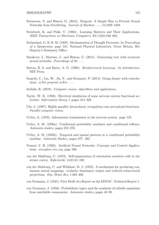


![Glossary 161
are called transactions and are designed to maximize the separability of the
descriptors on different classes while reduces the intra-class distances. xiv, 15,
160
HSL The HSL color space is a typical representation of colors in a cylindrical coor-
dinate system. In this representation the lightness is codified in the height of
the cylinder, the hue in the rotation of the rotation, and the saturation with
the distance from the center axis. xiv, 93, 161
HSV The HSV color space similar to HSL, however, the lighting is represented with
the variable value and is distributed in a different manner. While in the HSL
the white is equaly distributed on the top surface of the cylinder, in the HSV
the white is in the exact center of the top surface. xiv, 93, 161
hyperbolic tangent function It is a sigmoid function with negative and positive
values on the negative and positive side respectively. It has asymptotic be-
haviour towards −1 and 1, and it can behave locally as linear or as a step
function. For that reason, it has been extensively used as activation functions
in Artificial Neural Networks (ANNs). 43
ICA The Independent Component Analysis (ICA) is a technique used in signal
processing to find additive subsignals that are non-Gaussian and statistically
independent. xiv, 86, 161
Infomax The maximum mutual information (Infomax) is an optimization principle
that tries to minimize the amount of information needed to codify a match
between a set of inputs and outputs. This principle has been studied in some
biological systems and has been applied on information retrieval and machine
learning algorithms. xiv, 83, 86, 87, 161
inverse problem It is a class of problems where the objective is to model a physical
system given a set of measurements. 6, 9
K-cells The Koniocellular cells (K-cells) are a type of ganglion cells with their
body in the retina of the eyes and with axons that extends to the LGN and
the primary visual cortex. In the LGN they are situated in the strates between
P-cells and M-cells. xiv, 30, 161
LGN The Lateral Geniculate Nucleus (LGN) is a section of the thalamus focused
on the visual system. It receives the axons of ganglion cells from the retina
through the optic nerve and optic chiasma and propagates their signals to the
primary visual cortex. xiv, 27, 30, 31, 33, 132, 161–163
LoG The Laplacian of Gaussian (LoG) is a blob detector based on the Laplacian
of a Gaussian. xiv, 11–13, 29, 161
logistic function Is a type of sigmoid function with values [0, 0.5] on the negative
side and values [0.5, 1] on the positive side. 43, 162](https://image.slidesharecdn.com/146c407b-3fa0-4973-a3fa-401852309d94-160905130833/85/mscthesis-185-320.jpg)


![164 Glossary
steps on time. These networks have been used succesfully for time series
predictions. xiv, 36, 55, 56, 85, 158, 160, 163
SGD The Stochastic Gradient Descent (SGD) is an optimization method for min-
imizing the error of an objective function. It is based on minimizing the error
in individual samples and estimates that the total error also decreases. One
requisite to apply this technique is that the objective function has be differen-
tiable. xv, 52, 53, 164
SIFT Scale-Invariant Feature Transform (SIFT) is an algorithm to extract a set of
important points from an image invariant to scale and translation. See the
Section 2.4.1 for an extended description. xv, 12–14, 59, 160, 163, 164
sigmoid belief network A sigmoid belief network is a directed and acyclic graph,
where the output of each node computes a logistic function given the binary
states of its parents. 87, 88
sigmoid function Mathematical functions with “S” shape, commonly monotoni-
cally increasing and with assymptotic behaviour at both ends. 43, 161
simple linear regression It is a technique to fit linearly a set of samples of a
dependent variable given a single explanatory variable. 39
SNARC The SNARC (Stochastic Neural Analog Reinforcement Calculator) was
one of the first hardware implementations of an Artificial Neural Network
(ANN), developed by Marvin Lee Minsky in the 50s. It was a set of bacum
tubes with random connections, and able to learn automatically. xv, xviii, 73,
164
softmax function The softmax function is a function that reduces a finite vector
of real values to a vector of the same size with values in the interval [0, 1]. It
uses the exponential function and a normalization factor to each element of
the vector. 43
SOM Self-Organizing Maps (SOMs) are a type of ANNs trained using unsupervised
learning to embed a complex feature representation in a reduced dimensional-
lity space (commonly two dimensions). The embedding is achieved by using a
competitive learning algorithm that computes a neighbourhood function be-
tween the samples and the different neurons, increasing the connectivity to the
winning neuron and its neigbours and decreasing it to the rest. They are also
known as Kohonen maps as the Finnish professor Teuvo Kohonen designed
them in the 1980s. xv, 37, 79, 82–84
SURF The Speeded-Up Robust Features (SURF) is an image descriptor similar to
Scale-Invariant Feature Transform (SIFT) but modified for a faster computa-
tion. xv, 14, 59, 164](https://image.slidesharecdn.com/146c407b-3fa0-4973-a3fa-401852309d94-160905130833/85/mscthesis-188-320.jpg)