The document presents a comprehensive analysis of sepsis management in the ICU, outlining its pathology, clinical overview, and the effectiveness of various scoring systems. It also discusses advanced quantitative analysis techniques, including algebraic statistical models and generative kernels, for mortality prediction. Additionally, it emphasizes the role of statins in sepsis incidence and outcomes, concluding with a summary of contributions and future work related to sepsis research.

1. On the Intelligent Management of Sepsis in the
Intensive Care Unit
Vicent J. Ribas Ripoll
e-mail: vribas@lsi.upc.edu
Supervisors: Dr. Alfredo Vellido Alcacena
Dr. Enrique Romero Merino
Soft Computing Research Group
LSI-Department (Artificial Intelligence Section)
Universitat Politècnica de Catalunya
October 25, 2012

2. O Rose, thou art sick!
The invisible worm
That flies in the night,
In the howling storm,
Has found out thy bed
Of crimson joy:
And his dark secret love
Does thy life destroy.
William Blake
2

3. Contents
1 Introduction 15
1.1 Motivation . . . . . . . . . . . . . . . . . . . . . . . . . . . . . . 16
1.2 Thesis Objectives . . . . . . . . . . . . . . . . . . . . . . . . . . . 16
1.3 Considerations about the Analysed Datasets . . . . . . . . . . . . 17
1.4 Expected Contributions . . . . . . . . . . . . . . . . . . . . . . . 18
1.5 Thesis Structure . . . . . . . . . . . . . . . . . . . . . . . . . . . 18
2 Medical Background: The Sepsis Pathology 21
2.1 Phylogenetic Overview . . . . . . . . . . . . . . . . . . . . . . . . 22
2.2 Historic Overview . . . . . . . . . . . . . . . . . . . . . . . . . . . 23
2.3 Clinical Overview . . . . . . . . . . . . . . . . . . . . . . . . . . . 26
2.3.1 Definitions . . . . . . . . . . . . . . . . . . . . . . . . . . 26
2.4 Systems for Scoring the Severity of Sepsis . . . . . . . . . . . . . 29
2.4.1 Sequential Organ Failure Assessment Score . . . . . . . . 30
2.4.2 Acute Physiology and Chronic Health Evaluation II . . . 30
3 State of the Art: Quantitative Analysis of Sepsis 35
3.1 Quantitative Analysis of the Pathophysiology of Sepsis . . . . . . 35
3.2 Quantitative Analysis of the Prognosis of Sepsis . . . . . . . . . . 37
3.3 Limitations of Existing Quantitative Analysis . . . . . . . . . . . 39
4 Background: Algebraic Statistical Models, Algebraic Exponen-
tial Families and Generative Kernels 41
4.1 Polynomial Representation: Outline in Three Examples . . . . . 41
4.1.1 Linear and Polynomial Regression . . . . . . . . . . . . . 42
4.1.2 Interpolation . . . . . . . . . . . . . . . . . . . . . . . . . 42
4.1.3 Polynomial Representation of a Univariate Gaussian Vari-
able . . . . . . . . . . . . . . . . . . . . . . . . . . . . . . 43
4.2 Algebraic Models . . . . . . . . . . . . . . . . . . . . . . . . . . . 44
4.2.1 Division . . . . . . . . . . . . . . . . . . . . . . . . . . . . 46
4.2.2 Gröbner Bases . . . . . . . . . . . . . . . . . . . . . . . . 47
4.2.3 Algorithm for Polynomial Regression/Interpolation of Ob-
servation Matrices . . . . . . . . . . . . . . . . . . . . . . 48
4.3 Regular Exponential Families . . . . . . . . . . . . . . . . . . . . 50
4.3.1 Important Properties of Regular Exponential Families . . 50
4.3.2 Discrete Distributions as Regular Exponential Families . . 51
4.3.3 Gaussian Distributions as Regular Exponential Families . 52
4.4 Algebraic Exponential Families . . . . . . . . . . . . . . . . . . . 52
3

4. 4.4.1 Semi-Algebraic sets . . . . . . . . . . . . . . . . . . . . . . 53
4.4.2 Independence Models and Algebraic Exponential Families 54
4.4.3 Factorization of Discrete Distributions and Graphical Mod-
els . . . . . . . . . . . . . . . . . . . . . . . . . . . . . . . 56
4.4.4 Markov Random Fields and Graphical Models . . . . . . 56
4.5 Kernels: Definitions and Properties . . . . . . . . . . . . . . . . . 59
4.5.1 Important Properties of Positive and Negative Definite
Kernels . . . . . . . . . . . . . . . . . . . . . . . . . . . . 60
4.5.2 Relation between Positive and Negative Definite Kernels . 61
4.5.3 Reproducing Kernel Hilbert Spaces . . . . . . . . . . . . . 62
4.5.4 Kernels as Covariance Functions . . . . . . . . . . . . . . 62
4.6 Generative Kernels from Algebraic Statistical Models . . . . . . . 64
4.6.1 Quotient Basis Kernel . . . . . . . . . . . . . . . . . . . . 64
4.6.2 Fisher Kernel for Exponential Families . . . . . . . . . . . 65
4.6.3 Kernels based on the Jensen-Shannon metric . . . . . . . 66
5 Background: Methods for Regression, Classification and Di-
mensionality Reduction 69
5.1 Regression Trees . . . . . . . . . . . . . . . . . . . . . . . . . . . 69
5.2 Classification Techniques . . . . . . . . . . . . . . . . . . . . . . . 71
5.2.1 Logistic Regression: Classification as Binomial Regression 71
5.2.2 Support Vector Machines . . . . . . . . . . . . . . . . . . 71
5.2.3 Classification with Feature Selection: Relevance Vector
Machines . . . . . . . . . . . . . . . . . . . . . . . . . . . 75
5.3 Dimensionality Reduction . . . . . . . . . . . . . . . . . . . . . . 77
5.3.1 Feature Selection Methods . . . . . . . . . . . . . . . . . . 77
5.4 Feature Extraction Methods . . . . . . . . . . . . . . . . . . . . . 77
6 Graphical Models of Sepsis Incidence and Outcome Prediction
in Patients Treated with Statins 81
6.1 Introduction . . . . . . . . . . . . . . . . . . . . . . . . . . . . . . 81
6.2 Materials . . . . . . . . . . . . . . . . . . . . . . . . . . . . . . . 82
6.3 Methods . . . . . . . . . . . . . . . . . . . . . . . . . . . . . . . . 82
6.3.1 Algebraic Statistical Models . . . . . . . . . . . . . . . . . 82
6.3.2 Models of Conditional Independence . . . . . . . . . . . . 83
6.3.3 Markov Random Fields . . . . . . . . . . . . . . . . . . . 83
6.3.4 Algebraic Interpolation from Gröbner Bases . . . . . . . . 84
6.4 Results . . . . . . . . . . . . . . . . . . . . . . . . . . . . . . . . . 85
6.4.1 Study of the Incidence of Sepsis with Bayes Networks over
the basal SOFA Score . . . . . . . . . . . . . . . . . . . . 85
6.4.2 Marginal Dependence Between Preadmission Use of Statins
and the ICU Outcome . . . . . . . . . . . . . . . . . . . . 85
6.4.3 Study of the Protective Effect of Preadmission Use of
Statins with MRFs . . . . . . . . . . . . . . . . . . . . . . 90
6.4.4 Study of Interactions by means of Algebraic Interpolation 91
6.4.5 Study of the Protective Effect of Preadmission Use of
Statins with Regression Trees . . . . . . . . . . . . . . . . 92
6.4.6 Study of Septic Shock Incidence with Regression Trees . . 93
6.5 Conclusion . . . . . . . . . . . . . . . . . . . . . . . . . . . . . . 94
4

5. 7 Severe Sepsis Mortality Prediction Using an Interpretable La-
tent Data Representation 97
7.1 Introduction . . . . . . . . . . . . . . . . . . . . . . . . . . . . . . 97
7.2 Materials . . . . . . . . . . . . . . . . . . . . . . . . . . . . . . . 97
7.3 Results . . . . . . . . . . . . . . . . . . . . . . . . . . . . . . . . . 98
7.3.1 Diagnosis of the Factor Analysis Model . . . . . . . . . . 98
7.3.2 Factor Interpretation from a Clinical Viewpoint . . . . . . 100
7.3.3 Mortality prediction using logistic regression over 14 factors101
7.3.4 Comparison with Logistic Regression over a Selection of
the Original Variables . . . . . . . . . . . . . . . . . . . . 103
7.3.5 Comparison with the APACHE II Mortality Score . . . . 104
7.4 Conclusions . . . . . . . . . . . . . . . . . . . . . . . . . . . . . . 104
8 Severe Sepsis Mortality Prediction from Observed Data 107
8.1 Introduction . . . . . . . . . . . . . . . . . . . . . . . . . . . . . . 107
8.2 Materials: Detailed Description of Generative Kernels . . . . . . 108
8.2.1 Quotient Basis Kernel . . . . . . . . . . . . . . . . . . . . 108
8.2.2 Fisher Kernel for Exponential Families . . . . . . . . . . . 110
8.2.3 Kernels based on the Jensen-Shannon metric . . . . . . . 111
8.3 Results . . . . . . . . . . . . . . . . . . . . . . . . . . . . . . . . . 112
8.3.1 Mortality Prediction with RVM . . . . . . . . . . . . . . . 112
8.3.2 Comparison with Shrinkage Feature Selection Methods for
Logistic Regression . . . . . . . . . . . . . . . . . . . . . . 113
8.3.3 Mortality Prediction with Generative Kernels . . . . . . . 114
8.4 Conclusions . . . . . . . . . . . . . . . . . . . . . . . . . . . . . . 116
9 Conclusions 119
9.1 On the Incidence of Sepsis and Coadjutant Factors to be Taken
into Consideration . . . . . . . . . . . . . . . . . . . . . . . . . . 120
9.2 Summary of Prognosis Indicators Obtainend and Their Accuracy 121
9.3 Summary of Mortality Predictors and Their Accuracy . . . . . . 121
9.4 Contributions . . . . . . . . . . . . . . . . . . . . . . . . . . . . . 123
9.4.1 Methodological Contributions . . . . . . . . . . . . . . . . 123
9.4.2 Clinical Contributions . . . . . . . . . . . . . . . . . . . . 123
9.5 Publications . . . . . . . . . . . . . . . . . . . . . . . . . . . . . . 124
9.5.1 Publications Directly Linked to this PhD Thesis . . . . . 124
9.5.2 Relevant Information Related to this PhD Thesis . . . . . 124
9.6 Outline for Future Work . . . . . . . . . . . . . . . . . . . . . . . 125
A General Considerations of Topology and Measure Theory 127
A.1 Topological Spaces . . . . . . . . . . . . . . . . . . . . . . . . . . 127
A.2 Measures . . . . . . . . . . . . . . . . . . . . . . . . . . . . . . . 129
A.3 Entropy and Divergences . . . . . . . . . . . . . . . . . . . . . . 130
5

6. 6

7. List of Figures
2.1 phylogenetic tree for the IRAK-3 Inflammation Toll Receptor . . 24
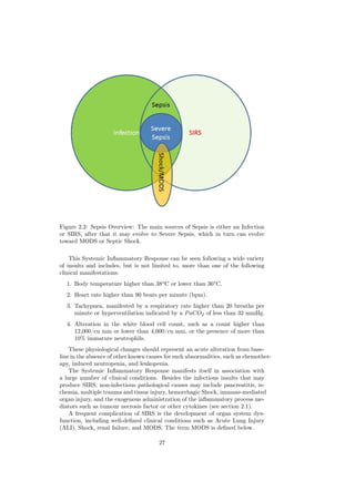
2.2 Sepsis Overview: The main sources of Sepsis is either an Infection
or SIRS, after that it may evolve to Severe Sepsis, which in turn
can evolve toward MODS or Septic Shock. . . . . . . . . . . . . . 27
2.3 APACHE II Table . . . . . . . . . . . . . . . . . . . . . . . . . . 33
5.1 Hyperplane through two linearly separable classes. . . . . . . . . 72
5.2 Graphical Representation of the Factor Analysis Model F12,10 . 79
6.1 APACHE II threshold selection: The blue curve represents
the true APACHE II mortality rate, whilst the smooth red curve
is the APACHE II mortality rate interpolated with a cubic poly-
nomial. The arrow points to the first inflection point of the
polynomial, which, in this study, corresponds to the selected
APACHE II threshold for stratification (i.e. APACHE II = 21).
This means that APACHE II scores lower than this threshold are
set to 2 in our MRF. Conversely, the APACHE II values higher
than 21 are set to 1 in our MRF. This threshold is consistent with
standard clinical practice [1] . . . . . . . . . . . . . . . . . . . . . 86
6.2 SOFA Score threshold selection: The blue curve represents
the true SOFA SCORE mortality rate, whilst the smooth red
curve is the SOFA Score mortality rate interpolated with a cubic
polynomial. As in the previous figure, the arrow points to the
first inflection point of the polynomial, which is selected as SOFA
Score threshold for stratification (i.e. SOFA = 7). This means
that SOFA scores lower than this threshold are set to 2 in our
MRF. Conversely, the SOFA values higher than 7 are set to 1
in our MRF. This threshold is consistent with standard clinical
practice. . . . . . . . . . . . . . . . . . . . . . . . . . . . . . . . . 87
6.3 Regression Tree for Probability of Survival. . . . . . . . . . . . . 94
6.4 Regression Tree for Shock Prediction . . . . . . . . . . . . . . . . 94
A.1 Two points separated by open sets in a Haussdorff Space . . . . . 129
7

8. 8

9. List of Tables
2.1 SOFA Score table adapted from [2]. Here, MAP stands for Mean
Arterial Pressure, DPM for dopamine, DBT for dobutamine, AD
for adrenaline, and NAD for Noradrenaline. Dosages are given in
[µg/Kg · min]. . . . . . . . . . . . . . . . . . . . . . . . . . . . . 31
4.1 Contingency Table for Gröbner Basis . . . . . . . . . . . . . . . . 48
6.1 List of SOFA scores, with their corresponding mean and standard
deviation values. . . . . . . . . . . . . . . . . . . . . . . . . . . . 83
6.2 Ranks of Minors Obtained with SVD . . . . . . . . . . . . . . . . 88
6.3 Ranks, H0 : {X1 } ⊥ {X2 }|{X3 }, {X4 } . . . . . . . . . . . . . . .
⊥ 88
6.4 Ranks, H0 : {X1 } ⊥ {X3 }|{X2 }, {X4 } . . . . . . . . . . . . . . .
⊥ 89
6.5 Ranks, H0 : {X2 } ⊥ {X3 }|{X1 }, {X4 } . . . . . . . . . . . . . . .
⊥ 89
6.6 Ranks, H0 : {X2 } ⊥ {X4 }|{X1 }, {X3 } . . . . . . . . . . . . . . .
⊥ 90
6.7 Ranks, H0 : {X3 } ⊥ {X4 }|{X1 }, {X2 } . . . . . . . . . . . . . . .
⊥ 90
6.8 Marginal Probabilities for ICU results . . . . . . . . . . . . . . . 91
7.1 List of SOFA scores, with their corresponding mean and standard
deviation values for the population under study (scoring organ
dysfunction). . . . . . . . . . . . . . . . . . . . . . . . . . . . . . 98
7.2 List of variables used in this study. . . . . . . . . . . . . . . . . . 99
7.3 Loadings Matrix: |Λ(i, j)| > quantile 95 for Factor fi are pre-
sented in bold. . . . . . . . . . . . . . . . . . . . . . . . . . . . . 102
7.4 Results for LR over Latent Factors with 10-fold cross validation . 103
7.5 Results for LR with 10-fold cross validation . . . . . . . . . . . . 103
8.1 Results for Shrinkage Methods . . . . . . . . . . . . . . . . . . . 114
8.2 Results for SVM with Generative Kernels . . . . . . . . . . . . . 116
8.3 p-value table for the Wilcoxon Rank Sum Test. The null hypoth-
esis tested is that the cdf for the resulting error distributions for
each kernel are different . . . . . . . . . . . . . . . . . . . . . . . 116
9.1 Summary of attributes, the dataset where they are used and their
calculation. . . . . . . . . . . . . . . . . . . . . . . . . . . . . . . 122
9.2 Summary of Prognosis Indicators and their Corresponding Accu-
racies . . . . . . . . . . . . . . . . . . . . . . . . . . . . . . . . . 123
9

10. 10

11. Abstract
The management of the Intensive Care Unit (ICU) in a hospital has its own,
very specific requirements that involve, amongst others, issues of risk-adjusted
mortality and average length of stay; nurse turnover and communication with
physicians; technical quality of care; the ability to meet patient’s family needs;
and avoid medical error due rapidly changing circumstances and work overload.
In the end, good ICU management should lead to an improvement on patient
outcomes.
Decision making in the ICU environment is a real-time challenge that works
according to very tight guidelines, which relate to often complex and sensitive
research ethics issues. Clinicians in this context must act upon as much available
information as possible, and could therefore, in general, benefit from at least
partially automated computer-based decision support based on qualitative and
quantitative information. Those taking executive decisions at ICUs will require
methods that are not only reliable, but also, and this is a key issue, readily
interpretable. Otherwise, any decision tool, regardless of its sophistication and
accuracy, risks being rendered useless.
This thesis addresses this through the design and development of computer
based decision making tools to assist clinicians at the ICU. It focuses on one of
the main problems that they must face: the management of the Sepsis pathology
(i.e. the systemic inflammatory response to a confirmed infection). Sepsis is
one of the main causes of death for non-coronary ICU patients. Its mortality
rate can reach almost up to one out of two patients for septic shock, its most
acute manifestation. It is a transversal condition affecting people of all ages.
Surprisingly, its definition was only standardized two decades ago as a systemic
inflammatory response syndrome with confirmed infection.
The research reported in this document deals with the problem of Sepsis
data analysis in general and, more specifically, with the problem of survival
prediction for patients affected with Severe Sepsis. The tools at the core of the
investigated data analysis procedures stem from the fields of multivariate and
algebraic statistics, algebraic geometry, machine learning and computational
intelligence.
Beyond data analysis itself, the current thesis makes contributions from a
clinical point of view, as it provides substantial evidence to the debate about the
impact of the preadmission use of statin drugs in the ICU outcome. It also sheds
light into the dependence between Septic Shock and Multi Organic Dysfunction
Syndrome. Moreover, it defines a latent set of Sepsis descriptors to be used as
prognostic factors for the prediction of mortality and achieves an improvement
on predictive capability over indicators currently in use.
11

12. 12

13. Acknowledgments
This PhD is essentially multidisciplinary since we are dealing with a difficult
medical issue through machine learning and algebraic modelling.
First and foremost, I would like to thank Dr. Angela Nebot for accepting
me to the Soft Computing group as a PhD student. I am mostly indebted to
my PhD supervisors Drs. Alfredo Vellido and Enrique Romero for their great
advice, support and constructive criticism.
From the clinical side, I would like to express my gratitude to Dr. Francisco
de la Torre and Dr. Jordi Rello for granting me access to the ICU at Hospital
Vall d’Hebron and letting me work with their exceptional team of doctors. I
would also like to thank Drs. Ruíz-Rodríguez and Caballero for sharing with me
their knowledge about Sepsis and also for their inconditional support in drafting
the clinical studies that had to be approved by Hospital’s Etical and Scientific
Committee. They have provided the patient data and also revised the clinical
part of this document and showed even more patience when I presented them
the most technically difficult and abstract concepts of this PhD.
I am also indebted to Dr. Marta Casanellas because she opened to me the
world of algebraic modelling. I had been very reluctant to take her course in
algebraic modelling in genomics during my MSc in Mathematical Engineering.
Had it not been for this course and its professor, I would have never thought
about the Quotient Basis Kernel or understood the role of statins during Sepsis.
I am convinced that my research will be related to Algebraic Statistics for a very
long time.
I would also like to thank my parents (Vicent and Maria Neus) for supporting
me during most part of my studies and for giving me the values of hard work
and patience. I would also like to thank most of my teachers from school and
highschool for nurturing my curiosity and impressing on me the pleasure of
knowledge. As one of them used to say (Mr. Lluís Busquets): “estudiar es
relacionar”.
And last but not least, I would like to express my deepest gratitude to my
wife, Maria José, who has been the source of inspiration for this PhD thesis. This
is definitely the result of her ability to come up with really difficult problems
and her capacity to give a turn in the point of view of addressing them. She
really managed to make me believe that Math must meet Medicine. I should
also thank her for the patience that she has shown during these long years. I
hope she will forgive all the time and weekends that I have stolen from her as
well as our three children: Vicent, Mar and Diana. If it had not been for their
love and support, I would have never been able to complete this PhD.
13

14. 14

15. Chapter 1
Introduction
¿Y si antes de empezar lo que hay
que hacer, empezamos lo que
tendríamos que haber hecho?
Mafalda
Sepsis is one of the main causes of death for non-coronary ICU (Intensive
Care Unit) patients. It is a transversal condition affecting people of all ages and,
more particularly, immunocompromised patients, critically ill patients, post-
surgery patients, AIDS patients, and the elderly. In western countries, septic
patients account for as much as 25% of ICU bed utilization and occurs in 1% -
2% of all hospitalizations. The mortality rates range from 20% for Sepsis and
40% for Severe Sepsis, to over 60% for Septic Shock.
Septic response and the Systemic Inflammatory Response Syndrome (SIRS)
can be portrayed as being one of the main contributing factors to around 200,000
deaths per year only in the United States. Moreover, this condition has pre-
sented a clear upwards trend for the last 20 years resulting in around 300,000
cases per year in the United States. The high rates of Severe Sepsis in west-
ern societies may be due to the ageing population, the increasing longevity of
patients with chronic diseases and the relative high frequency with which Sep-
sis develops in patients with AIDS (immunocompromised patients) and those
patients who have received an organ transplant or undergone complex surgery.
One of the main complications of the Septic Shock is that it may result in
Cardiogenic Shock. Cardiovascular dysfunction resulting from Septic Shock and
Cardiogenic Shock require immediate resuscitative efforts to prevent progressive
end-organ damage and death. The diagnosis of Septic Shock is not trivial and it
is usually carried out in challenging clinical emergency situations. Early recogni-
tion of signs of decreased perfusion before the onset of hypotension, appropriate
therapeutic response, and removal of the center of the infection are the keys to
survival of patients with Septic Shock. Given the criticality of Septic Shock, it
is of capital importance to have available an early indication of this condition
in order to allow doctors to act rapidly at the onset of Sepsis.
Needless to say, the ICU environment can be an unforgiving one in terms of
decision making tasks. Clinicians in general might benefit from at least partially
automated computer-based decision support, but those clinicians making real-
time executive decisions at ICUs in particular will require methods that are not
15

16. only reliable, but also, and this is a key issue, readily interpretable. This thesis
aims to address these needs through the design and development of computer-
based decision making tools to assist clinicians at the ICU. These developments
will focus on the problem of Sepsis in general and, more specifically, on the
problem of survival prediction for patients with Severe Sepsis. The tools of
Sepsis data analysis in this work stem form the fields of multivariate statistics,
algebraic statistics, algebraic geometry, machine learning and computational
intelligence.
1.1 Motivation
From what has been stated above, one may conclude that Sepsis is the result of
the uncontrolled inflammatory response to infection. At this stage it is also very
important to note that, today, Sepsis is a health state that can only be assessed
with certainty a posteriori (i.e. when the condition has already taken place),
but at the same time requires action to be taken immediately and, whenever
possible, preventively [3, 4]. Extensive research efforts have been made to study
Sepsis from a proteomics point of view (a good overview on this topic can
be found in [5]), but as of today the results are so far inconclusive and cost-
effectiveness of specific treatments such as Drotrecogin alpha (activated) (Xigris
TM
, Elli Lilly) is still under debate [6]. For this reason, it is extremely important
to provide simple and readily interpretable tools to manage Sepsis and improve
its prognosis.
This becomes even more important when taking into account that the ICU
is an extremely data intensive environment. Monitoring ranges from beat-to-
beat (Blood Pressure, Heart Rate or ECG), hours (gas exchange, white blood
cell count, lactate), to days (Apache, SOFA, Dynamic SOFA). The aggregated
data storage requirements for a patient can be of several Gigabytes, if we take
into consideration all biomedical signals. It is therefore understandable that any
new parameter to be measured in the ICU must provide high value in terms of
prognosis and interpretation (i.e. must be associated with and complementary
to the pathophysiology and management of Sepsis).
Moreover, there is a non-trivial relation between the parameters and clinical
traits mentioned above and the different types and degrees of Sepsis that can be
statistically estimated. It is also possible that different machine learning tech-
niques can be employed to identify these relations and improve the management
of the Septic patient. More particularly, the continuation of some preadmission
treatments during the ICU stay may have a significant impact on outcome.
In conclusion, there is a clear need to develop/modify the analytical tools for
studying the prognosis of septic patients and also improve the sensitivity and
specificity capabilities of the scores already available and currently in use in clin-
ical practice, whilst keeping the overall complexity of such tools at a reasonable
and practical level.
1.2 Thesis Objectives
The main objectives of this PhD thesis are:
1. Improving our knowledge about the incidence of Sepsis. Although the
16

17. incidence of Sepsis is, in general, very well documented [3] (c.f. section
6.4.1) there is still some controversy about the real incidence of Sepsis in
Spain. For example, this is one of the main issues of contention at the
Hospital in which the data analysed in this thesis were generated, given
the fact that they only see and therefore control the most severe cases of
Sepsis (while the less severe are managed in the general ward).
2. Improving the understanding of Sepsis physiology and inferring functions
that describe the relationship of measured variables with the state of Sepsis.
According to the definitions of Sepsis given in the following chapters, there
is a clear difference between Multiple Organ Failure Syndrome (MODS)
and Septic Shock. However, very seldom does one see a pure Septic Shock
without MODS (Multi Organ Dysfunction Syndrome). In other words,
there must be a dependence between them and it is this relation that
must play an important role in the prognosis and management of sepsis.
3. Studying the time evolution of Sepsis with respect to several manage-
ment/measurement variables. The main results of the Surviving Sepsis
Campaign (SSC) have also been controversial [7] due to the fact that some
studies also show that the most important factors from the SSC are the
timely administration of antibiotics and performance of haemocultures.
Given the fact that the ICU that we collaborate with is quite compliant
with the SSC, we plan to evaluate the impact of these guidelines in ICU
outcome and detect which ones are the most predictive.
4. Developing a system that could provide prognostic indicators of mortality
related to Sepsis, with high reliability, at the onset of the pathology. The
most important indicators of Sepsis (SOFA and APACHE II) are calcu-
lated at admission to the ICU. However, there are other variables that may
play an important role in the prognosis of Sepsis. Here we plan to detect
the underlying factors that explain the ICU prognosis model and also per-
form attribute selection procedures, which may complement those used in
clinical practice (backward and forward feature selection in linear/logistic
regression).
1.3 Considerations about the Analysed Datasets
This PhD thesis analyses two main datasets. More specifically, the first two
databases come from two independent prospective studies approved by the Clin-
ical Investigation Ethical Committee of the Vall d’Hebron University Hospital
in Barcelona, Spain. The data for these two studies was collected by the Group
on Shock, Organic Dysfunction and Resuscitation (SODIR) of Vall d’Hebron’s
Intensive Care Unit (VH-ICU).
The first dataset is described in detail in chapter 6 and is devoted to studying
the impact of the preadmission use of statins on the prognosis of Sepsis. This
dataset is extremely valuable not only because it is far larger than any other
reported in the literature (see chapter 6), but also because it is accompanied
by the most important scores at admission. This dataset has enabled us to put
the preadmission use of statins in the context of severity and organ dysfunction,
17

18. which clearly have an impact on the interpretation and disparity of results found
in the literature.
The second dataset is presented in chapter 7 and covers the time span be-
tween June 2007 and December 2010. This dataset includes 354 patients. At
this stage it is also important to note that this dataset is affected in its number
of patients by the flu pandemic that took place during autumn/winter 2010.
1.4 Expected Contributions
The expected contributions of this thesis are twofold. From a clinical point of
view, it is expected to clarify and shed some light onto the debate about the
impact of the preadmission use of statins in the ICU outcome, and show the
dependence between Septic Shock and Multi Organic Dysfunction Syndrome
(MODS). Also, from a clinical point of view it is expected to obtain a latent
model-based set of descriptors of sepsis, which could be used as prognostic
factors for the prediction of mortality due to Sepsis. And last but not least, it
is also expected to improve the overall accuracy of already existing prognostic
indicators widely used by the clinical practice by means of variable selection,
shrinkage methods and generative kernels.
From a machine learning point of view, it is expected to study the depen-
dence relations between the different variables by means of Algebraic Statistical
Models. These models, put in context of the Regular Exponential Families, will
enable us to re-parametrize the probability distribution functions by means of
polynomial ideals on an algebraic variety. Although this approach has been
successfully deployed in phylogenetics (where different models are used to study
the mutations between genes), in the approach followed in this thesis, transition
matrices are calculated and parametrized from the available data. We also use
a very powerful theorem (Hammersley Clifford) to study the marginal depen-
dence between variables and obtain the associated graphical models. Finally, we
show that the Algebraic Statistical Models for the Regular Exponential Family
over a metric space (Haussdorff) induce a convex-dual space that can be used
to derive Generative Kernels by means of a re-parametrization of the cumulant
generation function to the negative entropy.
1.5 Thesis Structure
This thesis is organized as follows:
• Chapter 2 presents an overview of Sepsis from three different perspec-
tives. First of all, we provide a philogenetics overview, which shows that
Sepsis is a cross-species syndrome and therefore as old as mankind. Sec-
ondly, we present an historic overview, starting from the first documented
case of sepsis in Plutarch. In this section, we also present the most mod-
ern definitions of Sepsis as a continuum (i.e. Infection, Inflammatory
Response, Sepsis, Severe Sepsis, Shock and Multi Organic Dysfunction).
This chapter is closed with a description of the Sepsis scoring systems
most widely used in clinical practice.
18

19. • Chapter 3 is devoted to a State of the Art of current quantitative and
qualitative methods for the assessment of the pathophysiology and prog-
nosis of Sepsis using machine learning techniques.
• Chapter 4 is mostly technical and provides the necessary background
for Algebraic Statistical Models and Generative Kernels. In this chapter,
graphical models are presented as a particular case of Algebraic Models.
In this chapter we also present a new kernel derived from Quotient Bases
of Algebraic Models.
• Chapter 5 provides the required background for the classification, regres-
sion and feature selection methods that we used throughout the thesis for
the study of Sepsis.
• Chapter 6 is devoted to the study of the incidence of sepsis and the im-
pact of preadmission use of Statins on the ICU outcome for septic patients.
This study starts with an analysis of conditional dependence between the
input variables, followed by a study of outcomes by means of algebraic
models, algebraic interpolation, Graphical Models and Classification and
Regression Trees.
• Chapter 7 presents our approach to Severe Sepsis Mortality prediction
using an interpretable latent data representation (obtained through Fac-
tor Analysis). First we provide a latent description of our input dataset
by means of Factor Analysis. The extracted factors are then used to cal-
culate a logistic regression model for mortality prediction. This logistic
regression model is compared against clinically well established state of
the art methods.
• Chapter 8 deals with the application of shrinkage methods (for dimen-
sionality reduction) with Relevance Vector Machines for the assessment
of Risk of Death (ROD) and also sets all the kernels defined in Chapter
4 in action. Given that the resulting (reduced) dataset is consistent with
standard clinical practice, it shall be used later on to study other ROD
predictors based on Kernel Methods.
• Chapter 9 presents the conclusions of this PhD thesis, the publications
and the main contributions (methodologic and clinical)
19

20. 20

21. Chapter 2
Medical Background: The
Sepsis Pathology
The world, unfortunately, rarely
matches our hopes and
consistently refuses to behave in a
reasonable manner.
Stephen Jay Gould
As mentioned in the introduction, Sepsis is one of the main causes of death
for non-coronary ICU patients. According to [3], it is the tenth most common
cause of death. Its mortality rates can reach up to 45.7% for septic shock, its
most acute manifestation. For these reasons, the prediction of the mortality
caused by sepsis is an open and relevant medical research challenge.
In western countries, septic patients account for as much as 25% of ICU
bed utilization and occurs in 1% - 2% of all hospitalizations. The statistics for
Catalonia (the Spanish region where the analysed data was collected) do not
differ from those presented above and septic patients account for 25% of bed
occupation at ICUs and PICUS (Pediatric ICUs), while approximately two-
thirds of septic cases take place in patients hospitalized for other illnesses.
The high rates of Severe Sepsis in western societies may be due to the age-
ing population, the increasing longevity of patients with chronic diseases and
the relative high frequency with which Sepsis develops in patients with AIDS
(immunocompromised patients) and those patients who have received an organ
transplant or undergone complex surgery. According to [4], the widespread use
of antibiotics, glucocorticoids, invasive catheterism and other mechanical de-
vices (such as mechanical ventilation and extra-corporeal circulation) also play
a role in the onset of Sepsis, Severe Sepsis and Septic Shock.
Patients clinically suspected of infection, an abnormal temperature and
tachycardia may be diagnosed with Septic Shock if they develop at least one
of the following manifestations of decreased organ perfusion: altered mental
status, oliguria, delayed capillary refill, bounding peripheral pulses or increased
lactate level. These clinical signs take place before hypotension. Decreased
blood pressure is a late sign of Septic Shock. Early recognition of signs of
decreased perfusion before the onset of hypotension, appropriate therapeutic
21

22. response, and removal of the center of the infection are key to the survival of
patients with Septic Shock. Given the criticality of this pathology, the avail-
ability of an early indication of the condition is of capital importance in order
to allow doctors to act rapidly at the onset of Sepsis.
Sepsis is the local or systemic response [4] to microbiotic agents (bacteria,
virus or fungus) traversing the epithelial barriers and invading the tissue un-
derlying. The main signs of SIRS (Systemic Inflammatory Response) include
fever, tachycardia and peripheral vasodilation (i.e. the inflammatory triad) as
well as hypothermia, leukocytosis or leukopenia and tachypnea. The symptoms
outlined above are commonly seen in patients with benign viral or bacterial
infections that respond to management with antipyretics or antibiotics or both.
However, signs of hypoperfusion (i.e. decreased blood flood through an organ)
suggest the possibility of early Septic Shock.
According to [4]:
“SIRS may have an infectious or a non-infectious aetiology. If
infection is suspected or proved, a patient with SIRS is said to have
Sepsis.”
If Sepsis was associated with the dysfunction of organs distant to the site of
infection, then the patient would be diagnosed with Severe Sepsis. Like Septic
Shock, Severe Sepsis is associated with both hypotension and hypoperfusion.
The impossibility of correcting the hypotension by means of fluid infusion, leads
to a diagnosis of Septic Shock. As Sepsis progresses to Septic Shock, the risk of
dying increases substantially. Sepsis can be reversed while patients with Septic
Shock often pass away despite aggressive therapy.
The complications associated with Sepsis can be summarized as follows:
• Cardiopulmonary complications: hypoxaemia, increased pulmonary water
content, decreased capillary refill, hypovolemia, acute respiratory distress
syndrome (ARDS) and depression of myocardial function.
• Renal complications: decreased urine output, azotemia, proteinuria and
non-specific urinary casts.
• Coagulation complications: thrombocytopenia, endothelial injury or mi-
crovascular thrombosis.
• Neurological complications: altered mental status, irritability, decreased
interaction, sleepiness or stupor.
• Vascular complications: decreased perfusion, bounding pulses, brisk cap-
illary refill, low diastolic blood pressure and wide pulse pressure.
2.1 Phylogenetic Overview
Most septic patients (about 70%) whose data was analysed in this thesis are res-
piratory cases. Most pulmonary cells express a large repertoire of genes under
transcription control that are modulated by biomechanical forces and bacterial
infections. Essential components of the innate immune system are the toll-like
receptors (TLRs), which recognize not only microbial products but also degra-
dation products released from damaged tissue providing signals that initiate
22

23. inflammatory responses. Several different components are involved in TLR sig-
nalling, such as IL-1 receptor-associated kinases (IRAK), which results in the
activation of pro-inflammatory cytokines, such as TNF-α and IL-6. Current ev-
idence indicates that IRAK-3 (also known as IRAK-M) is a negative regulator
of the TLR pathways and a master regulator of inflammatory processes during
Sepsis [8, 9, 10, 11, 12, 13]. This inflammatory mediated approach is a very ac-
tive field of research both from a clinical and proteomics point of view. However,
these IL approaches are still far from reaching widespread clinical practice.
Given that the genetic sequence of IRAK-3 is known for different species
(most primates and rodents), it is possible to reconstruct the phyologenetic
trees for these species [14]1 . Since the phylogenetic reconstruction by means of
four different data analysis approaches (Unweighed Pair Group Method with
Arithmetic Mean, Jukes-Cantor, Neighbour Joining and Maximum Likelihood
-a good overview of these methods can be found in [14]) clearly groups the
Homo Sapiens with the Macaque and Orangutan (see figure 2.1), it can be
concluded that these three species shared a common ancestor with a similar
IRAK-3 structure and, therefore, similar lung inflammation characteristics.
2.2 Historic Overview
From section 2.1, it can be concluded that Sepsis is at least as old as mankind.
About 4,000 years ago, the Egyptians postulated that the intestine contained
2
a dangerous ‘principle’, which they defined as WHDH and pronounced
‘ukhedhu’. This principle could find its way into the vessels, settle anywhere
in the body, or even ‘rise to the heart’ and kill [15].
The concept of WHDH makes sense, given that the intestines do, in fact,
contain dangerous substances. From the Egyptians onward, auto-intoxication
from the intestine has become a common explanation for certain pathologies.
The fear of WHDH led the Egyptians to search substances that never suffer
decay and, thus, may prevent it in wounds by means of sympathetic magic [16].
In fact, they devised some wound salves that were probably the best possible in
those days. At the top of the list is honey, which is not only aseptic but also a
powerful antiseptic.
Later on, in the 5th century BC, the ancient Greeks adopted or reinvented
the concept of auto-intoxication from the gut and elaborated on it. Our major
sources of information are the Hippocratic books, where we find two words,
which concern us: Sepsis (σ η ψις) and pepsis (π˜ψις). Although these two
˜
words cannot be translated exactly, they represented two different forms of
biological breakdown. Sepsis was very close to our concept of putrefaction and
implied a bad smell, whereas pepsis was a composite of ‘cooking’, ‘digestion’,
and ‘fermentation’. Both can occur inside the body and, medically, pepsis was
seen as helpful, whereas Sepsis was always dangerous. This later usage was also
supported by Aristotle [17].
However, one has to wait until ca. 100 AD to find the first documented case
of Sepsis. Among the essays included in Plutarch’s Morals (Vol. I Chapter XVI
and Vol. III, Book VI) [18] is one entitled Precepts on Health, which is often
1 Gene Data Source: http://www.ensembl.org/index.html
2 Even though they could not see the intestinal flora by any optical means.
23

24. Figure 2.1: phylogenetic tree for the IRAK-3 Inflammation Toll Receptor
24

25. cited by its Latin title De Tuenda Sanitate Praecepta. In Vol. I, Chapter XVI,
we find the following story:
“ [...] Niger, when he was teaching philosophy in Galatia, by
chance swallowed the bone of a fish; but a stranger coming to teach in
his place, Niger, fearing he might run away with his repute, continued
to read his lectures, though the bone still stuck in his throat; from
whence a great and hard inflammation arising, he, being unable to
undergo the pain, permitted a deep incision to be made, by which
wound the bone was taken out; but the wound growing worse, and
rheum falling upon it [it became purulent]3 , it killed him.”
Beyond the remarkable surgical procedure [19], what is of interest to us is the
fact that Niger’s death was not due to the operation but due to the consequent
infection. More particularly, what killed Niger was a post-surgical Sepsis, evi-
dence of which manifested itself at the surgical site on which Plutarch’s account
is clear.
The concept of Sepsis presented above was used until the 19th century and
there are few pathophysiological investigations known during these centuries. In
this regard, it is no surprise that the history of Sepsis is very much intertwined
with that of surgical procedures, antiseptics (such as iodine) and drug discovery
(the most outstanding being the discovery of antibiotics).
However, in the 17th century, a doctor in Leyden named Herrman Boerhave
postulated that toxic substances in the air were the cause for Sepsis. This theory
was further expanded in the 19th century by Justus von Liebig who stated that
it was the contact between wounds and oxygen that initiated the development
of Sepsis.
During the second half of the 19th century, an obstetrician at the Vienna
General Hospital, Ignaz Semmelweis, took a revolutionary approach to prevent-
ing the death caused by puerperal fever. His department had an especially high
mortality rate (18%) and he discovered that it was common practice for stu-
dents to examine pregnant women directly after pathology lessons. By that time
hygienic measures such as hand washing or surgical gloves were not customary
practice.
Semmelweis deducted that child bed fever was caused by “decomposed ani-
mal matter that entered the blood system” (recall the Egyptian principle out-
lined above). As a matter of fact, he succeeded in lowering the mortality rate
to 2.5 % by introducing hand washing with a chlorinated lime solution before
every gynaecological examination. However, in spite of the clinical success, the
hygienic measures were not accepted, and colleagues harassed him, being forced
to leave the city. It took him until 1863, more than 15 years after his findings, to
publish his work “Aetiology, terminus and prophylaxis of puerperal fever ” (Die
Aetiologie, der Begriff und die Prophylaxis des Kindbettfiebers). The failure to
achieve a professional reputation and the unrelenting opposition of the medi-
cal establishment may have facilitated the development of a psychiatric disease.
Semmelweis was eventually committed to a lunatic asylum where he died from
a wound infection probably as a result of the beatings he underwent there. It is
an irony of fate that he died from a disease that he dedicated his life to fight. It
was the surgeon Joseph Lister who managed to introduce the general procedure
3 The words within brackets have been added for interpretation purposes.
25

26. of instrument sterilization in medical practice. The methods initiated by Lister
are not very different from those applied today.
Arguably, the most important breakthrough regarding Sepsis is due to the
works of Louis Pasteur. Pasteur discovered that tiny cell organisms caused
putrefaction and termed these organisms as bacteria (see definitions of Sepsis
given below) and correctly deduced that these microbes could cause disease.
He also made the significant discovery that bacteria in fluids could be killed by
heating. This meant that a fluid could be sterilized.
At the beginning of the 20th century, the German physician H. Lennhartz
initiated the change in the understanding of Sepsis from the ancient concept
of putrefaction to the modern view of a bacterial disease. It was, however,
his student Hugo Schottmüller (1867-1936), who in 1914 paved the way for a
modern definition of Sepsis: “Sepsis is present if a focus has developed from
which pathogenic bacteria, constantly or periodically, invade the blood stream
in such a way that this causes subjective and objective symptoms”. Thus, for
the first time, the source of infection as a cause of Sepsis came into focus.
Although antiseptic procedures meant a huge medical breakthrough, it soon
became apparent that a number of patients still developed Sepsis. In this pre-
antibiotic time, the death rate was very high. These patients often showed
very low blood pressure. This condition was called Septic Shock. Only with
the introduction of antibiotics after WW II could the death rate of Sepsis be
reduced further. With technological progress, intensive care medicine started
to develop and Sepsis patients soon became the main patient fraction on ICUs
[20].
2.3 Clinical Overview
2.3.1 Definitions
In August 1991, the American College of Chest Physicians/Society of Critical
Care Medicine Consensus Conference took place with the goal of agreeing and
standardizing a set of definitions to be applied to patients with Sepsis and its
sequelae [21, 22], which is the reference mainly followed in this section. In this
conference, new terms were proposed and others (like septicaemia) were aban-
doned from clinical practice. Broad definitions for Sepsis and SIRS were also
proposed along with detailed physiologic parameters by which a patient could
be categorized. Definitions for Severe Sepsis, Septic Shock, hypotension, and
Multiple Organ Dysfunction Syndrome (MODS) were offered. These definitions
have since been deployed and provided a good framework for the treatment of
Sepsis. The aim of this subsection is to provide an overview of these definitions,
which shall be used throughout this thesis. Figure 2.2 presents a summarized
graph of the concepts outlined below.
Systemic Inflammatory Response Syndrome, Sepsis and Septic Shock
As stated above, Sepsis is defined as “the systemic response to infection”. It
is apparent that a similar, or even identical, response can arise in the absence
of infection. Therefore, the term “Systemic Inflammatory Response Syndrome”
(SIRS) is proposed to describe this inflammatory process, independent of its
cause.
26

27. Figure 2.2: Sepsis Overview: The main sources of Sepsis is either an Infection
or SIRS, after that it may evolve to Severe Sepsis, which in turn can evolve
toward MODS or Septic Shock.
This Systemic Inflammatory Response can be seen following a wide variety
of insults and includes, but is not limited to, more than one of the following
clinical manifestations:
1. Body temperature higher than 38o C or lower than 36o C.
2. Heart rate higher than 90 beats per minute (bpm).
3. Tachypnea, manifested by a respiratory rate higher than 20 breaths per
minute or hyperventilation indicated by a P aCO2 of less than 32 mmHg.
4. Alteration in the white blood cell count, such as a count higher than
12,000/cu mm or lower than 4,000/cu mm, or the presence of more than
10% immature neutrophils.
These physiological changes should represent an acute alteration from base-
line in the absence of other known causes for such abnormalities, such as chemother-
apy, induced neutropenia, and leukopenia.
The Systemic Inflammatory Response manifests itself in association with
a large number of clinical conditions. Besides the infectious insults that may
produce SIRS, non-infectious pathological causes may include pancreatitis, is-
chemia, multiple trauma and tissue injury, hemorrhagic Shock, immune-mediated
organ injury, and the exogenous administration of the inflammatory process me-
diators such as tumour necrosis factor or other cytokines (see section 2.1).
A frequent complication of SIRS is the development of organ system dys-
function, including well-defined clinical conditions such as Acute Lung Injury
(ALI), Shock, renal failure, and MODS. The term MODS is defined below.
27

28. When SIRS is the result of a confirmed infectious process, it is
termed Sepsis. In this clinical circumstance, the term Sepsis represents the
Systemic Inflammatory Response to the presence of an infectious agent. In this
regard, infection is defined as the microbial phenomenon characterized by an
inflammatory response to the presence of micro-organisms or the invasion of
normally sterile host tissue by those organisms. Bacteremia is the presence of
viable bacteria in the blood stream. The presence of viruses, fungi, parasites,
and other pathogens in the blood are described in a similar manner (i.e. viremia,
fungemia, parasitemia).
Sepsis and its sequelae represent a continuum of clinical and pathophysiolog-
ical severity. Of course, the degree of severity independently affects prognosis
(as shall be investigated in this thesis). Some clinically recognizable stages of
Sepsis include the following:
• Severe Sepsis: Sepsis associated with organ dysfunction, hypoperfusion
abnormality, or Sepsis-induced hypotension. Hypoperfusion abnormalities
include lactic acidosis, oliguria, and acute alteration of mental state.
• Sepsis Induced Hypotension: Presence of a systolic blood pressure of less
than 90 mmHg or a fall of 40 mmHg or more from the baseline in the
absence of other cause for hypotension (i.e. Cardiogenic Shock ).
• Septic Shock : A subset of Severe Sepsis (i.e. it includes organ dysfunc-
tion and is therefore very closely related to MODS, as it shall be seen
below), defined as Sepsis-induced hypotension and persisting despite ad-
equate fluid resuscitation (fluid administration), along with the presence
of hypoperfusion abnormalities or organ dysfunction. Patients receiving
inotropic or vasopressor agents may no longer be hypotensive by the time
they manifest hypoperfusion abnormalities or organ dysfunction. How-
ever, they would still be considered to suffer from Septic Shock.
Multiple Organ Dysfunction Syndrome
Multiple Organ Dysfunction Syndrome (MODS) is defined as the detection
of altered organ function in the acutely ill patient. The term dysfunction
identifies this process as a phenomenon in which organ function is not capable
of maintaining homeostasis (system stability). This process, which may be
absolute or relative, can be more readily identified as a continuum of change
over time for which it must be considered that:
1. It describes a continuum of organ dysfunction, although specific descrip-
tions of this continuous process are not currently available.
2. The recognition of early organ abnormalities must be improved so that
treatment can be initiated at early stages in the evolution of the syndrome.
3. Changes in organ function over time can be viewed as an important ele-
ment in its prognosis. When applied to MODS, existing measures of illness
severity provide only a snapshot in time of this dynamic process, and are
generally without reference to the natural course of disease.
4. It is subject to modulation by numerous factors at varying time periods,
both interventional- and host-related.
28

29. In the light of what has been said so far, MODS is understood to develop by
two relatively distinct, but not mutually exclusive, pathways. Primary MODS
is the direct result of a well-defined insult in which organ dysfunction occurs
early and is directly attributable to the insult itself (for example, as the result
of traumatic injury). In primary MODS, the participation of an abnormal and
excessive host inflammatory response in both the onset and progression of the
syndrome is not as evident as in secondary MODS.
Secondary MODS develops not as a result of the insult itself but, instead, as
the consequence of a host response and is identified within the context of SIRS.
SIRS is also a continuous process, and describes an abnormal host response
that is characterized by a generalized activation of the inflammatory reaction in
organs remote from the initial insult. Given that SIRS/Sepsis is a continuous
process, MODS may be understood to represent the more severe end
of the spectrum of severity of illness that characterizes SIRS/Sepsis.
Therefore, secondary MODS usually evolves after a latent period following the
inciting injury or event, and is most commonly seen to complicate severe infec-
tion.
2.4 Systems for Scoring the Severity of Sepsis
In normal clinical practice, and while treating the syndromes outlined in the
previous section, clinicians are always trying to catch up with the pathology. In
other words, they are treating severely ill patients at later stages of illness. It
is also apparent that many of these patients who have more complex illnesses
may be suffering from a combination of chronic and acute disease.
The rationale for using scoring systems in a clinical environment is to ensure
that the increased complexity of disease in patients currently being treated is
consistently represented for all those involved in the form of evaluations and
descriptions. A specific goal of severity scoring systems is to use these impor-
tant patient attributes to describe the relative risks of patients and identify
where along the continuum of severity the patient resides. This should reduce
the variability due to patient factors so that the incremental impact of new or
existing therapies can be more precisely determined. Also, more precise mea-
surements of patient risk should lead to new insights into disease processes and
serve as a tool with which clinicians could more accurately monitor patients and
implement the use of new therapies.
It is increasingly being recognized that the ultimate goal of severity scoring
can be more than just obtaining a figure representing the degree of physiological
disturbance. Severity scoring can be used in conjunction with other risk factors
such as disease aetiology to anticipate and estimate outcomes such as ICU mor-
tality. These estimates can be calculated at the time a patient presents for care
or for entry into a clinical trial. Therefore, they can serve as a pretreatment
protocol. They can also be updated during the course of therapy, thereby de-
scribing the course of illness and providing an alternative for the evaluation of
response. What follows is a summary description of some of the scoring systems
currently in use in medical procedure.
29

30. 2.4.1 Sequential Organ Failure Assessment Score
In 1994, the ESICM (European Society of Intensive Care Medicine) [2] organized
a consensus meeting in Paris to create a so-called Sequential Organ Failure As-
sessment (SOFA) Score with the aim of objectively and quantitatively describing
the degree of organ dysfunction/failure over time in groups of patients or even
individuals. The main two major applications of the SOFA score are:
1. Improving the understanding of the natural history of organ dysfunc-
tion/failure and the interrelation between the failure of various organs
/ systems.
2. Assessing the effect of new therapies on the course of organ dysfunc-
tion/failure. This could be used to characterize patients at admission
in the ICU (and even serve as an ICU entry criterion4 ), or to evaluate
treatment efficacy.
Originally, the SOFA score was not designed to predict outcome but to
describe a series of complications on the critically ill. Although any assess-
ment of morbidity is related to mortality to some extent, the SOFA score was
not designed just to describe organ dysfunction/failure according to mortality.
However, and as investigated in this thesis, SOFA scores greater than 7 could
present important ICU outcome prediction capabilities. Moreover, when com-
bined with additional parameters, it provides a very powerful set of features not
only for outcome assessment but also for the study of the evolution of Sepsis
into its more severe states. The latter is one of the main design objectives of
this particular score.
The SOFA limits the number of organs/systems under study to six, namely:
Respiratory (inspiration air pressure), Coagulation (Platelet Count), Liver (Bilir-
rubine), Cardiovascular (Hypotension), Central Nervous System (Glasgow Coma
Score), Renal (Creatinine or Urine Output). The scoring for each organ/system
ranges from 0 for normal function to 4 for maximum failure/dysfunction. The fi-
nal SOFA score is the addition of the dysfunction indexes for all organs/systems.
Therefore, the maximum possible SOFA score is 24, corresponding to maximum
failure for all of the six organs/systems considered. Table 2.1 shows the SOFA
Score calculation procedure.
In the light of what has been described so far and from a practical per-
spective, a SOFA score greater than 1 corresponds to Multiple Organ
Dysfunction Syndrome (MODS), while Cardiovascular SOFA scores
greater than 2 correspond to Septic Shock. Normally, SOFA scores are
calculated at ICU admission. However, daily calculations of SOFA scores (Dy-
namic SOFA) [23, 24] provide valuable information about organ dysfunction
evolution and prognosis. In our work, Dynamic SOFA was used to study the
evolution of Septic Shock and the derivation of ICU prognostic indicators.
2.4.2 Acute Physiology and Chronic Health Evaluation II
“Acute Physiology and Chronic Health Evaluation II” (APACHE II) is a severity-
of-disease classification system [1]. After admission to an ICU, an integer score
4 In this regard, during the 2010 flu pandemic in Australia, patients were admitted in the
ICU with a maximum SOFA score of 7.
30

31. SOFA Score Points 1 2 3 4
Respiration
P aO2 /F iO2 mmHg < 400 < 300 < 200 < 100
Coagulation
3
10
Platelet Count: Platelets× mm3 < 150 < 100 < 50 < 20
Liver
Bilirubine [mg/dL] 1.2-1.9 2.0-5.9 6.0-11.9 > 12
Cardiovascular
Hypotension MAP< 70 DPM DPM > 5 DPM > 15
or DBT ≤ 5 AD ≤ 0.1 AD > 0.1
NAD ≤ 0.1 NAD > 0.1
Central Nervous System
Glasgow Comma Score 13-14 10-12 6-9 <6
Renal
Creatinine [mg/dL] or 1.2-1.9 2.0-3.4 3.5 - 4.9 >5
Urine Output or < 500 ml/day < 200 ml/day
Table 2.1: SOFA Score table adapted from [2]. Here, MAP stands for Mean
Arterial Pressure, DPM for dopamine, DBT for dobutamine, AD for adrenaline,
and NAD for Noradrenaline. Dosages are given in [µg/Kg · min].
from 0 to 71 is computed for the patient on the basis of several measurements.
Higher scores imply a more severe disease and, therefore, a higher Risk of Death
(ROD).
APACHE II was designed to measure the severity of disease for adult patients
admitted to ICUs. The minimum age is not specified in the original study [1],
but it is commonly recommended using APACHE II only for patients older than
15 years. This scoring system is applied in different ways:
• Some procedures are only carried out in, and some drugs are only pre-
scribed to, patients with a given APACHE II score.
• The APACHE II score can be used to describe the morbidity of a patient
when comparing their outcomes with that of other patients.
• Predicted mortalities are averaged for groups of patients in order to specify
the group’s morbidity.
Even though newer scoring systems have replaced APACHE II in some in-
stances [25, 26], APACHE II continues to be used extensively in clinical practice,
due to its simplicity of calculation and the abundance of related medical docu-
mentation.
The score is calculated from 12 routine physiological measurements (such as
blood pressure, body temperature, heart rate, etc.) during the first 24 hours
after admission (see figure 2.3), plus information about previous health status
and some information obtained at admission (such as age). The resulting score
should always be interpreted in relation to the illness of the patient. Once the
initial score is determined within 24 hours of admission, no new score can be
calculated during the ICU stay. If a patient is discharged from the ICU and
31

32. readmitted, a new APACHE II score must be calculated. In this thesis, the
APACHE II score was used to assess patient severity and also as a baseline
measure for comparing ROD in Severe Sepsis.
32

33. 33
Figure 2.3: APACHE II Table

34. 34

35. Chapter 3
State of the Art: Quantitative
Analysis of Sepsis
No hay que empezar siempre por
la noción primera de las cosas que
se estudian, sino por aquello que
puede facilitar el aprendizaje.
Aristotle
Current research in quantitative analysis of Sepsis using physiological mea-
surements or standard scores is still at its very early stages. Different method-
ological approaches have been followed, with a diverse range of goals. Only a
few studies have recently started to make use of quantitative machine learning
and computational intelligence-related methods.
3.1 Quantitative Analysis of the Pathophysiology
of Sepsis
Although the pathophysiology of Sepsis is fairly well understood by the medical
community, the correlation between different clinical traits and the onset of
Sepsis has not yet been studied in detail. For example, Arterial Resistance,
Blood Flow, MAP and Reactive Hyperaemia and their relation to the severity
of Sepsis are studied in [27], while, in [28], neuroautonomic modulation of heart
rate and blood pressure were assessed in Sepsis or Septic Shock, concluding that:
“Uncoupling of the autonomic and cardiovascular systems occurs
over both short- and long-range time scales during Sepsis, and the
degree of uncoupling may help differentiate between Sepsis, Septic
Shock, and recovery states.”
Regarding the poor blood perfusion in tissue during Sepsis, a study by El-
lis and colleagues [29] built a model with partial differential equations of the
capillary network structure and oxygen transport from blood to tissue, and
described how experimental values relate to model parameters. The reported
35

36. simulations show the effects of Sepsis on oxygen transport heterogeneity and
the development of tissue hypoxia.
In a different study, Ross and co-workers [30] derived a system of ordinary
differential equations (modelled as a coupled system of three differential equa-
tions) together with an Artificial Neural Network (ANN) model of inflammation
and Septic Shock. These equations take into consideration three main param-
eters (namely, pathogen influence, immunological response and cell damage),
which are learned by means of an evolutionary approach (this approach is in-
dependent of the complexity of the objective functions) and, after that, four
models are selected by minimum description length.
A Fuzzy Decision Support System (DSS) for the management of post-surgical
cardiac intensive care unit (CICU) patients was described in [31]. The DSS
encompasses an input module to evaluate the patient’s hemodynamic status; a
diagnostic module that implements the expert decision-making strategies; and
a therapeutic module that incorporates a multiple-drug fuzzy control system
for the execution of the therapeutic recommendations. The DSS is validated
on a physiological model of the human cardiovascular hemodynamics whose
parameters have been modified to reproduce the key pathological features of
Sepsis.
Also in the field of the pathophysiology of Sepsis, it has been demonstrated
that mitochondrial nitric oxide synthase (mtNOS) plays an important role in
the onset of Septic Shock [32]. In turn, mtNOS is also related to ventricular
contractility and, therefore, to the cardiovascular complications of Sepsis. Re-
sults suggest that mtNOS may contribute to the ventricular depression during
Septic Shock.
There are also other inflammatory mediators during Septic Shock that may
result in ischemia or other cardiovascular complications. In particular, Septic
Shock has a direct impact in tissue perfusion and, therefore, in the most irrigated
organs such as the stomach. In the light of this condition, the gastric mucosa,
which can be monitored by means of gastric impedance spectroscopy, will de-
teriorate during a Septic Shock prior to MODS or ischemia, as investigated in
[33] and [34].
In addition to the articles described above, [35] presents an architecture for
multi-dimensional temporal abstraction and its application in Pediatric Inten-
sive Care Units (PICU). According to the authors, “temporal abstraction (TA)
provides the means to instil domain knowledge into data analysis processes and
allows transformation of low level numeric data to high level qualitative nar-
ratives. TA mechanisms have been primarily applied to uni-dimensional data
sources equating to single patients in the clinical context”. This architecture
enables the analysis of data arriving from a number of patients, as well as the
detection of several conditions within the PICU, including Sepsis.
Different papers in this field address the problem of rule generation [36]
[37]. It is argued in [36] that, due to the irregularities in patient data recording
at ICUs, it is worth exploring a generalization paradigm (i.e., individual cases
generalized to more general rules) rather than an association paradigm, which
combines single data attributes from an individual patient. The algorithm for
rule generation and classification presented in this work is based on heuristically
generated set-based data intersections in the development of Sepsis. On the
other hand, the approach in [37] entails embedding a rule generation algorithm
into a medical data mining cycle. The architecture of the system is improved
36

37. by means of a growing trapezoidal basis function network.
Beyond [37], there are other studies that deploy ANNs for the study of Sepsis.
Amongst them, [38] presented a clinical study examining SIRS and MODS in
the ICU after cardiac and thoracic surgery. The ANN-based prediction system
introduced in this work takes into consideration the time interval between the
onset of Sepsis and until the receding of the symptoms. Then, from this set of
observed data, an ANN that predicts the evolution of Sepsis into Severe Sepsis
is built. One of the main findings of this study is that there is a significant
correlation between the number of SIRS episodes and the outcome of Severe
Sepsis for each individual patient.
The initiatives related to the application of ANNs to the study of Sepsis have
also resulted in expert systems such as the one called SES, described in [39],
which was designed for the diagnosis of pathogens and prescription of antibiotics.
The performance of SES has been evaluated in [40] and improvements based on
the available knowledge-base clinical database have been proposed.
Support Vector Machines (SVM) have also been used for the prediction of
Sepsis. Kim et al. [41] applied them to study Sepsis in post-operative patients.
More specifically, they applied SVMs for regression and One-Class SVM for
studying the temporal evolution of Sepsis using data from 1,239 patients, re-
porting an AUC of 94% for the detection/prediction of Sepsis. This method has
also been used for the diagnosis of Sepsis. Wang et al. [42] built a DSS for the
diagnosis of Sepsis based on the following attributes: Age, Heart Rate, Body
Temperature, Respiration Rate, White Cell count and the APACHE II score.
This study reported an AUC of 88%, a sensitivity of 87%, and a specificity of
88%.
3.2 Quantitative Analysis of the Prognosis of Sep-
sis
The SIRS pathology is known to be a quite sensitive indicator of Sepsis [43], but
also one of poor specificity. Different studies have shown that the incidence of
SIRS is quite high in critical patients in general. For example, Pittet et al. [44]
presented a SIRS incidence of up to 93% in critical care patients, while Rangel
et al. showed an incidence of 68% [43]. The latter study also shows that 25%
of patients with SIRS developed a Sepsis, 18% presented Severe Sepsis, and 4%
of them, Septic Shock. Regardless of these incidence ratios, the early detection
of patients with a higher ROD remains a challenge.
The MEDS (Mortality in Emergency Department Sepsis) score is a collection
of variables routinely recorded in the emergency departments (terminal illness,
tachypnea/hypoxaemia, Septic Shock, platelet count, age, lower respiration in-
fection, bands, nursing home resident and mental status). It was shown in [45] to
yield an AUC of 0.88 for the population under study: patients at the emergency
department with SIRS (not taking into account those septic patients admitted
in the emergency department who were not critical enough to be admitted in
the ICU).
Since the publication in 1985 of the Organ System Failure (OSF) score by
Knaus [46], which is a prognosis scale to evaluate and quantify MODS, alterna-
tive prognostic scores have been developed. They include the already reviewed
37

38. APACHE II score [1], as well as the SOFA score [2], and the LODS (Logistic
Organ Dysfunction System) [47]. Two prognostic scores based on the PIRO
model (predisposition, insult/infection, response and organ dysfunction) have
also been recently proposed: the SAPS3 PIRO score ([48]: AUC 0.77) and the
PIRO score ([49]: AUC 0.70).
Machine learning methods have been used with varying success for the pre-
diction of mortality caused by Sepsis. A diagnostic system for Septic Shock
based on ANNs (Radial Basis Functions -RBF- and supervised Growing Neu-
ral Gas) was presented in [50], reporting an overall correct classification rate
of 67.84%, with a high specificity of 91.61%, but an extremely poor sensitivity
of 24.94%. Also in this area, Brause et al. [51] applied an evolutionary algo-
rithm to an RBF network (the MEDAN Project) to obtain, over a retrospective
dataset, a set of predictive attributes for assessing mortality for Abdominal Sep-
sis, namely Systolic and Diastolic blood pressure and thrombocytes. This study
reported an AUC of 0.90-0.92.
SVM methods have also been used in this context. Tang et al. [52] pre-
sented a SVM-based system for Sepsis and SIRS prediction from non-invasive
cardiovascular spectrum analysis, reporting an overall accuracy of 84.62%, with
a rather low specificity of 62.50% and a high sensitivity of 94.44%.
As described in previous sections, Sepsis can evolve into more critical condi-
tions (namely, Severe Sepsis and Septic Shock) and it can also result in the death
of the patient (60% for Septic Shock). Medical symptoms were modelled in [53]
as observations caused by the transitions in time in a Hidden Markov Model
(HMM), where each patient class (surviving or not) defines its own transition
probabilities between the states, especially to the death and dismissal state.
Therefore, at least two HMM models are derived: one for the surviving patients
and one for deceased. The diagnostic approach presented in this paper consists
of presenting the patient data to a system which computes the probability for
them to be either part of the surviving or the non-surviving HMM. According
to authors, the understanding of the underlying state transition probabilities
results in a “prediction probability success of about 91%”. This study goes be-
yond the clinical septic evolution described above and considers the different
evolution states during an episode of Septic Shock.
A predictor based on the physiological data available from the IMPACT
project1 was defined in [54]. It studies the correlations between HR, MAP, Body
Temperature and Respiration Rate, in order to distinguish between critically ill
adult patients with and without Sepsis in the first 24 hours of admission to an
ICU. This study concludes that MAP and Body Temperature are independently
related to the onset of Sepsis. However, this clinical viewpoint is more related to
the cardiovascular function and it is therefore more predictive of Severe Sepsis
and Septic Shock.
Also regarding HR monitoring, HR variability was studied in [55], and a
predictive model based on this parameter was developed in search of abnormal
HR characteristics (HRC) prior to neonatal Sepsis. The predictive model devel-
oped in this article is based on multivariate logistic regression models adjusted
for repeated measures, with the HRC values as predictor variables prior to the
deterioration on the condition of the newborn (i.e., CRASH: Cultures, Resus-
citation and Antibiotics Started Here). This article concludes that real-time
1 www.piccm.com
38

39. monitoring of HRC may result in early diagnosis and treatment of neonatal
Sepsis.
3.3 Limitations of Existing Quantitative Analysis
Sepsis is a clinical syndrome that can only be diagnosed a posteriori by the
concurrence of several clinical signs, as described in Chapter 2. This of course
imposes a great limitation to the different systems and approaches currently
used for ascertaining the presence of Sepsis. Despite this limitation, there is
still room for testing different clinical traits or even co-ocurrent factors that may
have an impact in the presence or prognosis of sepsis, which are not routinely
measured. It also believed that the application of Machine Learning techniques
may help in shedding some light on some open debates in the clinical practice.
For instance, one question that still lingers in the clinical literature is should
we stop or continue statins treatment during sepsis?. This is just but one open
problem/limitation to treatment that needs to be addressed.
Regarding the prognosis of Sepsis, and to the best of our knowledge, the best
one could do is to perform haemocultures and administer antibiotics during the
very first hours of evolution. Time of treatment is of paramount importance.
In this regard, one of the main limitations encountered is that the most widely
used indicators in clinical practice like the APACHE II 2 lack specificity despite
having an acceptable sensitivitity (0.82 sensitivity and 0.55 specificity). This
same specificity problem is found for the indicator tailored for Sepsis, namely
SAPS, with a sensitivity and specificity of 0.69. Finally, the indicator SOFA is
only related to organ failure and, therefore, does not provide ROD. However, it
is widely accepted that SOFA scores greater than 7 are associated with higher
mortality rates. This fact is also studied in this thesis.
Over the last years, the Lilly pharamaceutical company has been studying
a new treatment for named Xigris TM (see, for example [56] and [6]), which is
a recombinant of the human activated C protein. This protein clearly plays a
role in the inflammatory cascade and has become the first drug approved by the
U.S. Food and Drug Administration (FDA) and the European Agency for the
Evaluation of Medicinal Products for treatment of patients with Severe Sepsis.
Given the risks of this treatment, it has been approved for use in patients with
a high ROD ascertained, for example, by means of the APACHE II score [56].
Not only does this impose a further risk for patients detected as a false positive
(leading to low specificity) but also to the National Health Systems as a whole
due to the elevated costs of treatment (about 30.000 USD/day 3 ). There is a
clear need for timely detection of Sepsis (according to the PROWESS studies
[6], Xigris only works during the first hours of evolution) and also improving
specificity and sensitivity of the indicators available.
Some improvement has already been detected for given patient populations
(see [51] above), which presents an AUC of 0.90 for abdominal sepsis. Unfor-
tunately, this is one of the most easily detected forms of Sepsis, since it takes
place right after surgery in most of the cases, with clear symptoms (fever after
surgery). Therefore, most of the approaches analysed are either limited in terms
of patient base or base pathology (i.e. they only look at a certain stage of Sepsis
2 this indicator was been designed for assessing the ROD in the ICU and not just Sepsis
3 private conversation with Prof. Dr. Roger Mark, from MIT
39

40. like Shock or MODS). There are also limitations in terms of the study design:
prospective vs. retrospective. The latter being the most easily implemented,
but also the most disputable when it comes to the results. Regarding the vari-
ables or clinical factors involved, often little attention is paid to the clinical eye
(for example, decrease of SOFA score and extubation or decrease of lactate lev-
els are clear signs of good prognosis), while other variables are overlooked. We
do not advocate to follow this instinct blindfolded, but just put it to a test for
confirmation. It is also believed that the complexity of the syndrome at hand
calls for a more “generative” approach to ascertain the prognosis of Sepsis by
means of a set of attributes that give a clear context of the patient at a given
time.
40

41. Chapter 4
Background: Algebraic
Statistical Models, Algebraic
Exponential Families and
Generative Kernels
And now to something completely
different.
Monty Python
The aim of this chapter is to present the necessary mathematical framework
for the latter study of Sepsis by means of Algebraic Statistical Models in general
and the marginal dependence between variables in particular. It is this marginal
dependence study that shall be used later to derive the underlying relations and
Graphical Models by means of the Hammersley Clifford theorem. The mathe-
matical background presented in this chapter is used in chapters 6 and 8. These
chapters include the study the incidence of Sepsis in the geographic area covered
by the Vall d’Hebron University Hospital in Barcelona, Spain. This incidence
is modeled as a hidden variable in a graphical model. We also use the mathe-
matical approach presented in this chapter to derive a new generative kernel to
study the prognosis of Severe Sepsis. The main contributions of this section are
the Quotient Basis Kernel obtained from Gröbner bases, the simplified Fisher
kernel and the representation the kernels based on the Jensen-Shannon metric
in an algebraic context.
4.1 Polynomial Representation: Outline in Three
Examples
The aim of the following three examples is to intuitively introduce the algebraic
background that shall be formally described throughout this chapter and to
provide the main ideas that shall be used throughout this PhD thesis. The first
example provides the first (and most obvious) layer of algebraization, where
41

42. linear regression models in polynomial form are presented. This can be further
generalized to polynomial regression. In this regard, spline regression may also
be presented algebraically.
The second example is the most technical in the sense that not only does
it introduce the basics of interpolative polynomials, but also one of the main
issues that must be addressed in this thesis: that polynomial residuals on high
dimensions are not unique. The only way we have to guarantee uniqueness for
the expressions of our interpolation polynomials is through Algebraic Geometry.
Finally, it is this Algebraic Geometry machinery that will allow us to step
into the most abstract level of algebraization. The third example provides a
simple presentation of this level of abstraction where exponential family distri-
butions are treated as polynomials in parameter space (sometimes this is also
done in sample space) so that the algebraic description presented in this chapter
can used for this particular set of probability density distributions.
4.1.1 Linear and Polynomial Regression
In a general classification/regression problem, we are interested in obtaining a
response y from an input x. Let Ψ = (X1 , · · · , Xp ) be the matrix of inputs.
therefore
y = ωt Ψ (4.1)
where Ψ takes different forms depending on the problem/model at hand. For
example, if we have N points xi : i ∈ {1, . . . , N } of dimension p, an ordinary
least square regression problem, ω takes the form:
−1
ω = Ψt Ψ Ψt y (4.2)
where Ψ is the N × p observations matrix. Our ability to estimate the param-
eter vector ω under standard theory is equated with: Ψ is N × p full rank or
Rank(Ψ) = p < N where ω is a p-dimensional vector and N is the number of
design points. In another example, the one-dimensional polynomial regression
p−1
y(x) = ωj xj (4.3)
j=0
needs p independent design points 1 so that the matrix Ψ = (X1 , · · · , Xp ) has
full rank. Also for submodels with fewer than p terms, the Ψ matrix has full
rank.
4.1.2 Interpolation
Imagine that we observe three distinct points (ai , yi ) : i ∈ 1, . . . , 3 in a super-
vised learning experiment. It is easy to show that there is a unique quadratic
curve through these points [57]. Let us define the polynomial
d(x) = (x − a1 )(x − a2 )(x − a3 ) (4.4)
1 Intuitively these points are equivalent to design points in Experimental Design. These
p-dimensional points also live in the support of the underlying probability distribution.
42

43. whose zeros are the observed/support points. Any other polynomial p(x) run-
ning through the support points also fulfils p(xi ) = yi (for i = 1, 2, 3). Without
loss of generality we can write
p(x) = s(x)d(x) + r(x), (4.5)
where r(x) is the remainder when p(x) is divided by d(x). Since, by construction,
d(x) has ai as roots, it is obvious from the equation above that
yi = p(ai ) = r(ai ) , (i = 1, 2, 3). (4.6)
By construction, our polynomial p can be interpreted as an interpolation
function with value yi at the point ai or, also, as the function defined only on
the support points and again with value yi at ai for (i = 1, 2, 3). However, a
word of caution must be given should we use this argument in high dimensions
(>2) since the division operation and the remainder themselves are not unique
[57]. For this reason, we need to move into the field of Algebraic Geometry
in order to guarantee unique representations. This shall be done through the
definitions and theorems: term ordering, varieties, polynomial ideals, the Hilbert
Basis theorem and, finally, Gröbner bases.
4.1.3 Polynomial Representation of a Univariate Gaussian
Variable
In this third example, we show a more profound level of algebraization that will
be used throughout this thesis. Let X be a Bernoulli variable taking values
in the support {0, 1} with probability q. By the central limit theorem, after n
repetitions with n sufficiently large the sum of Bernoulli variables converge to
N (µ = nq, σ = nq(1 − q)), the raw interpolator of the logarithm for this variable
takes the form:
2π µ2 µ 1
p(x) = − log( )+ 2 + x − 2 x2 . (4.7)
σ 2σ σ2 2σ
The interpolator after exponentiation is
2π µ2 µ 1
p(x) = exp − log(
ˆ )+ 2 + x − 2 x2 . (4.8)
σ 2σ σ2 2σ
µ2 µ −1
Defining φ(η) = − log( 2π ) +
σ 2σ 2 , η1 = σ2 and η2 = 2σ 2 . Setting ζ0 =
eφ(η) , ζ1 = eη1 and ζ2 = eη2 and noticing that the support of our Bernoulli
distribution takes values on an integer grid, we have the representation
2
x x
p(x) = ζ0 ζ1 ζ2 .
ˆ (4.9)
This coincides with the form of the regular exponential family for a univariate
Gaussian
p(x) = exp η t T (x) − φ(η) (4.10)
where T (x) is the vector with components x and x2 . Later on we will see that
T (x) correspond to the sufficient statistics of a Regular Exponential Family.
43

44. These sufficient statistics shall be used as building blocks for our Generative
Kernels. The example shown here is very powerful in the sense that sets the
intuitive basis for the implicit representation of Regular Exponential Families
in the ring of polynomials. This result will be used to algebraically derive
the generative kernels using the sufficient statistics of the Regular Exponential
Family as the principal building block.
By now we should have noticed the deep interplay between different parametriza-
tions. In the next sections it will also become apparent that another parametriza-
tion is needed in terms of moments. These parametrizations become even harder
because statistical models or submodels are obtained by imposing restrictions
on the parameters. In this thesis we will define an Algebraic Statistical Model
(ASM) as one which adopts one of these parametrizations and for which the re-
strictions on the parameters themselves are also polynomial [57]. A more formal
definition of these ASM shall be given below. An important example of these
models are independence models, which force factorization of the raw polyno-
mial interpolators in parameter space and map additivity inside the exponential
representation and factorization in the ζ. Conditional independence models as
used in this PhD. are also examples of ASM.
4.2 Algebraic Models
In this section we present the definition of Algebraic Models as given in [57]
where factors or inputs are denoted by x, responses or outputs are denoted by
y, parametric functions denoted by η or functions of η. These are related by
polynomial algebraic relations, possibly implicit. Another feature of this defini-
tion is that constraints of polynomial type can be included in the specification
of the model. Implicit models and the introduction of constraints can lead to
the use of dummy variables.
The parameters of the model as interpreted in statistics are functions of any
form with the restriction that they belong to a specified field. For example
Q (η1 , . . . , ηp ) is the set of all rational functions in η1 , . . . , ηp with rational co-
efficients. Another example is Q eη , . . . , eη the set of all exponential rational
1 p
functions. Parameters are treated as unknown quantities and in most cases ap-
pear in linear form. The algebraic space used is the commutative ring of all
polynomials K[x1 , . . . , xs ] in the indeterminates x1 , . . . , xs and with coefficients
in the field K.
Definition 1. [57] An initial ordering is a total order on the indeterminates
x1 , . . . , x s .
When the indeterminates are indexed from 1 to s such as x1 , . . . , xs it is
convention to consider an initial ordering xi xi+1 ∀i = 1 . . . s − 1.
Definition 2. [57] The quantities of the form xα1 , . . . , xαs with αi ∈ Z+ ∀i =
1 s
1, . . . , s are called terms.
Definition 3. [57] The set of all terms in s indeterminates is denoted by
Term{s}.
For a given initial ordering a term is specified by the vector of length s of
its exponents. Therefore Term{s} is coded by Zs +
44

45. Definition 4. [57] Term Ordering
A term-ordering on K[x] is an ordering relation τ (or τ or ) on Term{s},
that is the terms of K[x] satisfying
1. xα 1 ∀xα with α = 0 and
2. ∀α, β, γ ∈ Zs such that xα
+ xβ , then xα xγ xβ xγ
Definition 5. [57] Let x1 , . . . , xs be indeterminates and let the initial ordering
be xi xi+1 ∀i = 1 . . . s − 1. The log operator is the function
log : Term {s} → Zs
+
(4.11)
xα = (xα1 , . . . , xαs ) → (α1 , . . . , αs )
1 s
For example, a valid term ordering for the polynomial f = −1/50xyz +
3/100xy + 9/100xz − 3/25yz − 21/100x + 27/100y + 8/25z + 7/25 is xyz xy
xz x yz y z 1. This polynomial is the interpolation polynomial
of the support points for our study on statins presented in this PhD Thesis.
Another example of term ordering for another polynomial would be x4 y 7 x4 y.
Definition 6. [57] Let τ be a term-ordering on K[x] and f a polynomial in
K[x]. The leading term of f , LTτ (f ) is the largest term with respect to τ among
the terms in f . The leading coefficient LCτ (f ) is the coefficient of LTτ (f ). The
leading monomial LMτ (f ) is the product LCτ (f )LTτ (f ).
For example, in our interpolation polynomial, the leading term LTτ (f ) is
xyz, the leading coefficient is LCτ (f ) −1/50 and the leading monomial LMτ (f )
is −1/50xyz.
Definition 7. [58] Monomials
A monomial in indeterminates t1 , . . . , tn is a formal expression of the form
tβ = tβ1 tβ2 · · · tβn , where β = (β1 , . . . , βn ) is the non-negative integer vector of
1 2 n
exponents.
Definition 8. [58] Polynomials
A polynomial f = β∈B cβ tβ is a linear combination of monomials where
the coefficients cβ are in a fixed field K and B ⊂ Zn is a finite set of exponent
+
vectors. The collection of all polynomials in the indeterminates t1 , . . . , tn with
coefficients in a fixed field K is the set K[t] = K [t1 , . . . , tn ]. The collection of
polynomials K[t] has the algebraic structure of a ring. Each polynomial in K[t]
is a formal linear combination of monomials, that can also be considered as a
function f : K → K, defined by evaluation. Throughout this thesis we will
focus on the ring R[x] of polynomials with real coefficients.
The notion of ordering and term-ordering is of capital importance to guar-
antee the uniqueness of our basis representations, interpolations and studies in
conditional independence.
Definition 9. [57] Variety
The algebraic variety of the finite set of polynomials f1 , . . . , fr in K[t1 , . . . , tn ]
is the set
Variety(f1 , . . . , fr ) = {(a1 , . . . , an ) ∈ Kn : fj (a1 , . . . , an ) = 0, j = 1, . . . , r}
(4.12)
45

46. Definition 10. [57, 58] Algebraic Model
Let K be a field, called the field of constants. Let K be a field of functions
φ : η → K, with η the set of parameters; K is called the field of parametric
functions. Let x = (x1 , . . . , xd ) be the control factors, y = (y1 , . . . , yp ) be the
responses and t = (t1 , . . . , th ) be the dummy variables. An algebraic model is
a finite list of polynomials f1 , . . . , fq , h1 , . . . , hl such that fi ∈ K[x, y, t] and
hj ∈ K[x, t]. The variety Variety (fi , hj : i = 1, . . . , q; j = 1, . . . , l) ∈ Kd+p+h is
called the model variety and the variety Variety(hj ) ∈ Kd+h is called the input
variety.
Definition 11. Algebraic Statistical Model
A statistical model that can be specified by means of a variety
Variety (f1 · · · fq , h1 · · · hl ) ∈ Kd+p+h
with respect to a set of parameters (with the ideal denoted by IdealVariety) is an
Algebraic Statistical Model.
Definition 12. Polynomial Ideal:
1. A polynomial ideal I is a subset of a polynomial ring K[x] closed under
sum and product by elements of K[x]. Specifically the set I ⊂ K is an ideal
if ∀f, g ∈ I and s ∈ K the polynomials f + g and sf are in I.
2. Let F be a set of polynomials. The ideal generated by F is the smallest
ideal containing F . It is denoted F .
3. An ideal I is radical if f ∈ I whenever a positive integer m exists such
that f m ∈ I.
√
4. The radical of an ideal I is the radical ideal defined as I = {f ∈ K : ∃m|f m ∈ I}
Definition 13. An ideal I is finitely generated if there exist f1 , . . . , fr polyno-
mials in K[x] such that for any f ∈ I there exist s1 , . . . , sr polynomials of K[x]
such that
r
f= si fi . (4.13)
i=1
We write I = f1 , . . . , fr and the set {f1 , . . . , fr } is called a basis of I.
Theorem 1. [57] Hilbert Basis Theorem
Every ideal in K[x] has a finite basis.
4.2.1 Division
The operations over K[x] are sum, products (with scalars and other polynomials)
and polynomial division. It is also of particular importance the simplification
of monomial fractions. Polynomial division may not be unique and requires the
notion of term-ordering as presented above. The following theorem summarizes
the division algorithm for univariate polynomials.
Theorem 2. [57] For every pair of polynomials, f and g in one indeterminate,
there exist unique polynomials sg , r such that LT(g) LT(r) and f = sg g +
r, where the leading terms are with respect to the only term ordering in one
dimension. The division algorithm returns sg and r.
46

47. In more dimensions the situation is less straightforward.
Theorem 3. [57] Let f, g1 , . . . , gt be in K[x] and τ a term-ordering. There exist
s1 , . . . , st ∈ K[x] and r ∈ K[x] such that
t
f= si gi + r (4.14)
i=1
and LTτ (r) is not divisible by any of the LTτ (gi )
4.2.2 Gröbner Bases
The Hilbert basis theorem 1 provides a very powerful result since it states
that any ideal is finitely generated (even if the generating set is not neces-
sarily unique). Another powerful result [57] is that this generation basis is of
a special type called Gröbner Basis, which we define below. These bases will
become essential in the derivation of regression/interpolation polynomials and
also for the algebraic derivation of the Fisher and Quotient Basis Kernels.
Definition 14. [57] Gröbner Basis
Let τ be a term ordering on K[x]. A subset G = g1 , . . . , gt of an ideal I is a
Gröbner basis of I with respect to τ iff
LTτ (g1 ), . . . , LTτ (gt ) = LTτ (I) (4.15)
where LTτ (I) = {LTτ (f ) : f ∈ I}.
Theorem 4. Given a term ordering, every ideal I except {0} has a Gröbner
basis and any Gröbner basis is a basis of I.
Let us formally define the Quotient Basis ESTτ that shall be used in the
algorithm presented in section 4.2.3 below.
Definition 15. [57] Quotient Basis
Let A be a set of unique support points and τ a term ordering. A monomial
basis of the set of polynomial functions over A is
ESTτ = {xα : xα ∈ LT(g) : g ∈ Ideal(A) }
/ (4.16)
This definition is stating that ESTτ comprises the elements xα that are not
divisible by any of the leading terms of the elements of the Gröbner basis of
Ideal(A) (c.f. Definition 25 ii) in [57]).
Theorem 5. [57] The set ESTτ has as many elements as there are support
points.
For example, imagine that we have the 3 × 8 contingency table 4.1 and that
we observe each support point with probability q 2 .
Let us recall, the example from section 4.1.2, where we interpolated three
points. Now the problem has increased a bit in complexity (from 3 to 8 points)
and we want to compute the vanishing ideal (in this case and the example), the
2 This is the table 6.8 obtained when we studied the dependence between preadmission use
of statins and outcome shall be further studied in chapter 6.
47

48. Table 4.1: Contingency Table for Gröbner Basis
x y z
1 1 1
2 1 1
1 2 1
2 2 1
1 1 2
2 1 2
1 2 2
2 2 2
Algebraic Model is defined by zero-dimensional Variety (i.e. the set of uniquely
observed points vanish in the Ideal). One way to calculate this vanishing ideal is
by means of the Buchberger Algorithm [14]. However, for a given set of points,
there is a more efficient algorithm based on specialized linear algebra techniques
for zero-dimensional ideals using Indicator Polynomials (i.e. a polynomial that
is 0 if x = a and 1 if x = 1). This algorithm is called M 3 after its inven-
tors (Marinari, Möller and Mora) [57],[59]. This method is implemented in the
CoCoA package [60, 61].
We have calculated the Ideal of table 4.1 with the function IdealOfPoints
[62] in ApCoCoA [61] and the lexicographic order. In our case the ideal is:
z 2 − 3z + 2, y 2 − 3y + 2, x2 − 3x + 2 , and its corresponding Gröbner basis
is: G = z 2 − 3z + 2, y 2 − 3y + 2, x2 − 3x + 2 . It is interesting to see that
this package constructs the Gröbner Basis equal to the Ideal (recall that every
Gröbner Basis G is also a basis of I) and also that the polynomials have as roots
1 and 2 (i.e. the coding values of our design matrix).
4.2.3 Algorithm for Polynomial Regression/Interpolation
of Observation Matrices
Now we are ready to integrate all the definitions and theorems given so far in
order to provide an algorithm for interpolation of designs or contingency tables
and regression (recall the second example in section 4.1.2). First of all, let us
summarize the following [63]:
• Let A = (X1 , · · · , Xp ) be an N × p observation matrix of N distinct
support points in Zp 3 . The N distinct points can be represented as the
set of solutions of the Gröbner Basis and a given term ordering τ (i.e.
the evaluation of the observation matrix through the polynomials of the
3 In section 4.3 we will further generalize the requirements for the distributions of these
input sets.
48

49. Grobner Basis): 
 g1 (A) = 0

 g2 (A) = 0

.
.


 .
gm (A) = 0

where G = {g1 , · · · , gm } is the Gröbner Basis of A.
• By the Hilbert Basis Theorem 1, for a given term ordering τ and ideal I
any polynomial p(x) can be written as
m
p(x) = Ij (A)gj (A) + r(A)
j=1
where r(A) is unique.
• The monomials of r(A) form a subset ESTτ , which comprises all mono-
mials not divisible by the leading terms of G for the given ordering τ .
Moreover, since r(A) is unique, ESTτ is also unique.
Now we are ready to give our algorithm for interpolation/regression 4 :
1. Input: matrix with unique points A and relative frequencies q. Without
loss of generality this matrix could also be a transformed version of A by
means of a Kernel.
2. Define a term ordering τ (for example lexicographic).
3. Calculate the ideal of matrix A (in our case, this is done with ApCoCoA)
[61].
4. Calculate the reduced Gröbner Basis G (this can be also calculated with
the function IdealOfPoints [62] in ApCoCoA).
5. Identify the subset ESTτ (i.e. identify the sub-set of monomials not di-
vided by G).
6. Let L be the logarithm of the monomials of ESTτ (i.e. exponents). Write
ESTτ = {aα }α∈L .
7. Write the polynomial interpolator as: p(a) = α∈L ηα aα .
8. Substitute the values of a in p(ak ) = qk k ∈ {1, . . . , N } and solve the
polynomial system for the parameters ηα . The solution is guaranteed and
unique by the construction of G.
For example, a valid interpolation polynomial for table 4.1 is f = −1/50xyz+
3/100xy+9/100xz−3/25yz−21/100x+27/100y+8/25z+7/25 and term ordering
xyz xy xz x yz y z 1. In this case, this interpolation is quite
straightforward provided that the contingency table is fully observed. These
polynomials become very useful for large contingency tables where we want to
interpolate unobserved states (for example, in genomics or proteomics).
4 The algorithm presented here goes beyond that presented in [63] in the sense that it is
not only limited to Experimental Designs and also provides the interpolated values for the
observed relative frequencies.
49

50. 4.3 Regular Exponential Families
Consider the sample space X with σ-algebra A on which a σ-finite measure υ
is defined. Let T : X → Rk be a measurable map [64, 65]. Define the natural
parameter space:
t
N = {η ∈ Rk : eη T (x)
dυ(x) < ∞}. (4.17)
X
For η ∈ N , we can define a probability density pη on X as
t
pη (x) = eη T (x)−φ(η)
, (4.18)
where
t
φ(η) = log eη T (x)
dυ(x) (4.19)
X
is the logarithm of the Laplace transform on υ t . Here t denotes matrix/vector
transpose. Let Pθ be the probability measure on (X , A) that has υ-density pη .
Define υ t = υ ◦ T −1 to be the measure that the statistic T induces on the Borel
σ-algebra of Rk . The support of υ t is the intersection of all closed sets A ⊆ Rk
that satisfy υ t (Rk A) = 0 [58].
Definition 16. Let k be a positive integer. The probability distributions (Pη |η ∈ N )
form a regular exponential family of order k if N is an open set in Rk and the
affine dimension of the support υ t is equal to k. The statistic T (x) that induces
the regular exponential family is called a canonical sufficient statistic.
Regular exponential families comprise the families of discrete distributions
and Gaussian distributions that are subject to the work of this PhD thesis.
4.3.1 Important Properties of Regular Exponential Fam-
ilies
Suppose X is a random vector that is distributed according to some unknown
distribution from a regular exponential family (Pη |η ∈ N ) of order k with canon-
ical sufficient statistic T (x). Given an observation X = x, the log likelihood
function takes the form:
l(η|T (x)) = η t T (x) − φ(η) (4.20)
where the log-Laplace function φ is a strictly convex and smooth function
over the convex set N .
Theorem 6. [66]Convexity Property:
1. N is a convex set and φ is convex on N.
2. φ is lower semi-continuous on Rk and is continuous on N 0 .
3. Pη1 = Pη2 iff the following convex combination is fulfilled:
φ(αη1 + (1 − α)η2 ) = αφ(η1 ) + (1 − α)φ(η2 ) (4.21)
for some α ∈ (0, 1). In this case 3 is valid for all α ∈ [0, 1].
50

51. 4. It the order of the exponential family is k (in particular, if Pη is minimal),
then ψ is strictly convex on N , and Pη1 = Pη2 for any η1 = η2 ∈ N .
Theorem 7. [66] Momentum Generation:
The derivatives of φ yield the moments of the canonical sufficient statistic
such as the expectation and covariance matrix:
d
ζ(η) = φ(η) = Eη {T (x)} (4.22)
dη
d2
Σ(η) = φ(η) = Eη {(T (x) − ζ(η))(T (x) − ζ(η))t } (4.23)
d2 η
4.3.2 Discrete Distributions as Regular Exponential Fam-
ilies
Let the sample space X be the set of integers {1, . . . , m}. Let υ be the counting
measure on X (the measure υ(A) of A ⊆ X is equal to the cardinality of A).
Consider the statistic T → Rm−1 ,
T (x) = (I{1}(x) , . . . , I{m−1}(x) )t , (4.24)
whose zero-one components indicate which value in X the argument x is
equal to. Also, when x = m, T (x) = 0. The induced measure υ t is a measure of
the Borel σ-algebra of Rm−1 with support equal to the m vectors in {0, 1}m−1
that have at most one non-zero component. The differences of these vectors
include all canonical basis vectors of Rm−1 . Thus the affine dimension of the
support υ t is equal to m − 1.
It holds for all η ∈ Rm−1 that
m−1
φ(η) = log 1 + e ηx <∞ (4.25)
x=1
The natural parameter space N is equal to all of Rm−1 and in particular is
open. The υ-density pη is a probability vector in Rm . The components pη (x)
for 1 ≤ x ≤ m − 1 are positive and given by
e ηx
pη (x) = m−1 ηx . (4.26)
1+ x=1 e
The last component of pη is also positive and equals
m−1
1
pη (m) = 1 − pη (x) = ηx
. (4.27)
x=1
1+ x=1 (m − 1)e
The family of the induced probability distribution Pη |η ∈ Rm−1 is a regular
exponential family of order m − 1. The interpretation of the natural parameters
ηx is one of log odds because pη is equal to a given positive probability vector
(p1 , . . . , pm ) if and only if ηx = log px − log pm for x = 1, . . . , m − 1. This
establishes a correspondence between the natural parameter space N = Rm−1
and the interior of the m − 1 dimensional probability simplex [58].
51

52. 4.3.3 Gaussian Distributions as Regular Exponential Fam-
ilies
Regarding Gaussian distributions, let the sample space X be the Euclidean
space Rp equipped with its Borel σ-algebra and Lebesgue measure υ. Let T :
X → Rp × Rp(p+1)/2 be given by:
t
T (x) = x1 , . . . , xp , −x2 /2, . . . , −x2 /2, −x1 x2 , . . . , −xp−1 xp
1 p . (4.28)
The polynomial functions that form the components of T (x) are linearly
independent and, therefore, the support of υ t has the full dimension p + p(p +
1)/2.
If η ∈ Rp × Rp(p+1)/2 ,write η[p] ∈ Rp for the vector of the first p components
ηi , 1 ≤ i ≤ j ≤ p and η[p×p] ∈ Rp × p for the symetric matrix defined by the
t
last p(p + 1)/2 components ηij , 1 ≤ i ≤ j ≤ p. The function x → eη T (x) is
υ-integrable if and only if η[ p × p] is positive definite. Therefore, the natural
parameter space N is equal to the Cartesian product Rp on the cone of positive
definite p × p matrices. If η is the open set N , then
1 t
φ(η) = −log det η[p×p] − η[p] η[p×p] η[p] − p log (2π) (4.29)
2
Now the Lebesgue densities pη can be written as
1
pη (x) = t
exp η[p] x − T r η[p×p] xxt /2 − η[p] η[p×p] η[p] /2 .
t
p −1
(2π) det η[p×p]
(4.30)
−1 −1
Setting Σ = η[p×p] and µ = η[p×p] η[p] , we find that
1 1 t
pη (x) = p exp − (x − µ) Σ−1 (x − µ) (4.31)
(2π) det (Σ) 2
is the density of the multivariate normal distribution Np (µ, Σ). Therefore,
the family of all multivariate normal distributions on Rp with positive definite
covariance matrix is a regular exponential family of order p + p(p + 1)/2 [58].
4.4 Algebraic Exponential Families
We know from definition 10 that a model that can be expressed by means of a
variety is a algebraic model. Taking this definition one step further (definition
11), a Statistical Model that can be expressed as a Variety is defined as an
Algebraic Statistical Model.
More formally, a statistical model [67] is a set of probability distributions
on the sample space S. A parameterized statistical model is a parameter set Θ
together with a function P : Θ → P (S), which assigns to each parameter point
θ ∈ Θ a probability distribution Pθ on S. Of course, by the definition above, Ex-
ponential Families are naturally defined as Statistical Models. Moreover, they
can be expressed by means of reparameterization as Algebraic Statistical Mod-
els (definition 11). Therefore, the statistical properties of exponential families
52

53. are determined by the geometry of their parameter spaces [58, 66]. This sug-
gests that if the parameter spaces have an algebraic structure then the tools of
computational algebraic geometry can be employed to address questions arising
in inference theory and Machine Learning. Semi-algebraic sets, as employed
in the following definition [58], provide the necessary flexibility to capture the
algebraic structure found in the models developed in this PhD thesis.
4.4.1 Semi-Algebraic sets
Loosely speaking a semi-algebraic set is simply a set that can be described with
a finite number of polynomial equalities and inequalities. A variety is clearly
a semi-algebraic set and also the interpolation polynomials and Gröbner bases
described above.
Definition 17. [58] A basic semi-algebraic set is a is subset of points in Rn of
the form
AF,H = {θ ∈ Rn | f (θ) > 0 ∀f ∈ F, h(θ) = 0 ∀h ∈ H} (4.32)
where F ⊂ R[t] is a finite (possibly empty) collection of polynomials and H ⊆
R[t] in an arbitrary (possibly empty) collection of polynomials. A semi-algebraic
set is a finite union of basic semi-algebraic sets. If F = ∅ then A is called a real
algebraic variety (see definition 9).
A general semi-algebraic set occurs when we consider sets of the form
AF,G,H = {θ ∈ Rn | f (θ) > 0 ∀f ∈ F, g(θ) ≥ 0, ∀g ∈ G, h(θ) = 0, ∀h ∈ H}
(4.33)
where both F and G are finite collections of real polynomials.
An example of a semi-algebraic set is the set of m × m positive definite
matrices Σ, where F consists of all principal sub-determinants of a symmetric
matrix Ψ and G, H are the empty set.
Definition 18. [58] Algebraic Exponential Family
Let (Pη |η ∈ N ) be a regular exponential family of order k. The subfamily
induced by the set M ⊆ N is an algebraic exponential family if there exists an
¯ ¯
open set N ⊆ Rk , a diffeomorfism g : N → N , and a semi-algebraic set A ⊆ Rk
−1
such that M = g (A ∩ N ¯ ).
The definition states that an algebraic exponential family is given by a semi-
algebraic subset of the parameter space of a regular exponential family. This
parameter space may be obtained by a re-parametrization g of the natural pa-
rameter space N .
Definition 19. [58, 68] Rational Mappings
f f
Let ψ1 = g1 , . . . , ψn = gn be rational functions where fi , gi ∈ R[x] =
1 n
R[x1 , . . . , xd ] are real polynomial functions. Then a rational map is defined
by:
ψ : Rd →, a → (ψ1 ((a), . . . , ψn ((a)) . (4.34)
The rational map is a well-defined function on the open set Dψ = {a ⊂ Rd :
gi (a) = 0}.
53

54. Theorem 8. [58] Tarski-Seidenberg
Let AF,H ⊆ Rd be a semi-algebraic set and ψ a rational map that is well
defined on AF,H , that is, AF,H ⊆ Dψ . Then the image ψ(AF,H ) is also semi-
algebraic set.
Definition 20. The open probability simplex is defined as
k
∆k−1 = (p1 , . . . , pk ) ∈ Rk : p1 , . . . , pk > 0 and pi = 1 (4.35)
i=1
Remark 1. [68] The open probability simplex for discrete random variables is
n−1
a basic semi-algebraic set, where F = {xi |i = 1, . . . , n − 1} {1 − i=1 xi }
and H = ∅. From a topological point of view, the relative interior of any con-
vex polyhedron in any dimension is a basic semi-algebraic set, while the whole
polyhedron is a basic semi-algebraic set.
Remark 2. [68] The set Σ ⊂ Rm×m of positive definite matrices is a basic semi-
algebraic set, where F consists of all principal sub-determinants of a symmetric
matrix Ψ, and G is the empty set.
4.4.2 Independence Models and Algebraic Exponential Fam-
ilies
The statistical models defined in this PhD thesis are based on conditional inde-
pendence considerations. In our case, we will study models for testing indepen-
dence hypothesis in contingency tables, which can be related to graphical models
by means of the Hammersley-Clifford Theorem such as Markov Chains or Lat-
tices. In this section, we show that conditional independence yields algebraic
exponential families for both the Gaussian and Discrete cases.
Ideals (see definition 12) can be used to determine real algebraic varieties by
computing the zero set of the ideal:
V (I) = {a ∈ Rn |f (a) = 0, ∀f ∈ I} . (4.36)
Reversing this procedure, if we are given a set V ⊂ Rn we can compute its
defining ideal, which is the set of polynomials that vanish on V :
I(V ) = {f ∈ R[x]|f (a) = 0, ∀a ∈ V } . (4.37)
Definition 21. [58] Invariant
Let A be a semi-algebraic set defining an algebraic exponential family PM =
{Pη |η ∈ M } via M = g −1 (A ∩ g(n)). A polynomial in the ideal I(A) is a model
invariant for PM .
Conditional independence can be studied by means of the definitions given
below.
Definition 22. [58] A set of indeterminates xi1 , . . . , xik is algebraically inde-
pendent for the ideal I if there is no polynomial in pi1 , . . . , pik that belongs to
I
Proposition 1. [58] The dimension of A is the cardinality of the largest set of
algebraically independent indeterminates for I(A).
54

55. Conditional Independence for Gaussian Distributions
Let X = (X1 , . . . , Xp ) be a random vector with joint normal distribution
Np (µ, Σ) with mean vector µ ∈ Rp and positive definite covariance matrix Σ.
For three pairwise disjoint index sets A, B, C ⊆ {1, . . . , p}, the sub-vectors XA
and XB are conditionally independent given XC , in symbols XA ⊥ XB |XC , iff
⊥
det ΣA C×B C = 0. (4.38)
Here A C × B C is the minor related to the variables over which we
are calculating the marginal dependence/independence (i.e. the resulting minor
after removing the rows and columns corresponding to the conditional indepen-
dence statement).
If C = ∅, then conditional independence given X∅ is understood to mean
marginal independence XA and XB . Here, equation 4.38 gives the semi-algebraic
set that allows to see the conditional independence for a Gaussian distribution
as an algebraic exponential family [58, 68].
For example, let X = (X1 , X2 , X3 ) have a trivariate normal distribution
N3 (µ, Σ) and define a model requiring X1 ⊥ X2 |X3 . This model is an algebraic
⊥
exponential family given by the subset M = ζ −1 (V ∩ ζ(N )), where ζ(N ) is the
Gaussian mean parameter space and the algebraic variety is:
A = (µ, Σ) ∈ R3 × R3×3 | det(σ{1,3}×{2,3} ) = σ12 σ3,3 − σ13 σ23 = 0 .
sym (4.39)
Conditional Independence for Discrete Data
Let a set of discrete random variables X1 , . . . , Xn where Xi takes values over the
probability space Ξi . Then a distribution over the sample space Ξ1 × · · · × Ξn
is equivalent to a matrix (pi1 ,...,in ) ∈ Ξ1 × · · · × Ξn where pi1 ,...,in = P rob(X1 =
i1 , . . . , Xn = in ).
Definition 23. Given three disjoint subsets A, B, C = ∅ of {X1 , . . . , Xn }, A
is independent of B given C, A ⊥ B|C if P rob(A = a, B = b|C) = P rob(A =
⊥
a|C = c)P rob(B = b|C = c) ∀a, b, c such that P rob(C = c) > 0.
Proposition 2. A probability distribution P = (pi1 ,...,in ) satisfies A ⊥ B|C iff
⊥
Pa,b,c Pa ,b ,c = Pa,b ,c Pa ,b,c .
∀a, a ∈ xi ∈A Ξi ,
(4.40)
∀b, b ∈ xj ∈B Ξj ,
∀c ∈ xk ∈C Ξk ,
where
Pa,b,c = P rob(A = a, B = b, C = c)
Pa ,b ,c = P rob(A = a , B = b , C = c)
(4.41)
Pa,b ,c = P rob(A = a, B = b , C = c)
Pa ,b,c = P rob(A = a , B = b, C = c).
Proof. We want to show Eq.(4.40), so we rewrite:
P (a, b|c)P (c)P (a , b |c)P (c) =
P (a, b |c)P (c)P (a , b|c)P (c).
55

56. Taking into account definition 23, the left hand side of this equation becomes
P (a, b|c)P (a , b |c) = P (a|c)P (b|c)P (a |c)P (b |c)
whereas, also by definition 23, its right hand side becomes
P (a, b |c)P (a , b|c) = P (a|c)P (b |c)P (a |c)P (b|c),
and, thus, the proposition holds. We are only left now to show that proposition
2 implies definition 23. For this, note that
P (A = a|C = c)P (B = b|C = c) =
P (a, b |c)P (a , b|c) =
b ,a
P (a, b |c) P (a , b|c)
b a
P (a, b|c)P (a , b |c) =
b ,a
P (a, b|c) P (a , b |c) = P (a, b|c).
a ,b
Definition 24. The conditional independence ideal IA⊥
⊥B|C is generated by all
quadratic polynomials in proposition 2
Equivalently, this definition implies that the rank of Mc is ≤ 1 where:
Pa,b,c Pa,b ,c
Mc = , (4.42)
Pa ,b,c Pa ,b ,c ∀c∈ Ξk
xk ∈C
which, as in the Gaussian case, gives the semi-algebraic set that allows us to
check marginal independence for the algebraic exponential family.
4.4.3 Factorization of Discrete Distributions and Graphi-
cal Models
A very important consequence of proposition 2 for multinomial distributions is
that conditional independence models can be compactly modelled by graphical
models via the Hammersley Clifford theorem, which also lend significant savings
to the computational tasks via factorization of the joint distribution. In this
section we introduce the definition of Undirected Graphical Models or Markov
Random Fields [69].
4.4.4 Markov Random Fields and Graphical Models
Definition 25. [69] Graph Separation
Given an undirected graph G = (V, E) where V and E are the set of nodes
and edges respectively, let A, B, C be disjoint subsets of nodes. If every path
from A to B includes at least one node from C, then C is said to separate A
from B in G.
56

57. Definition 26. [69] Markov Random Field
Given and undirected graph G, a Markov Random Field (MRF) is defined
as a set of probability distributions M RFG := {p(x) : p(x) > 0, ∀p, x} such that
∀p ∈ M RFG and for any three disjoint subsets A, B, C of G, if C separates A
from B then p satisfies XA ⊥ XB |XC . If p ∈ M RFG , we often say p respects
⊥
G.
With these two definitions [70] it is relevant to ask the following questions:
• Given a graph G and p ∈ M RFG , how can we efficiently check all the
conditional independence relationships encoded in it? This is normally
done by means of the independence definitions above that translate into
the Markov condition for Graphical Models (i.e. each node is independent
of its non-descendants).
• Given a set of conditional independence relationships, how can we obtain
a valid G? This is also done by means of studying the marginal indepen-
dences presented above.
• For all distributions in M RFG , how should their pdf look like? The Ham-
mersley Clifford theorem shows that these pdf should factorize as we will
show below.
Definition 27. [71] Cliques and Maximal Cliques
A clique of a graph is a sub-graph of it where each pair of nodes is connected
by an edge. The maximal clique of a graph is a clique which is not a proper
subset of another clique.
The set of maximal cliques is normally denoted by C.
Definition 28. [69, 71] Factorization
A pdf p(x) is said to factorize wrt a given undirected graph G it can be written
as:
1
p(x) = ψc (xc ), (4.43)
Z
c∈C
where ψc is a general non-negative real valued function called the potential func-
tion. The constant Z ensures p(x)dx = 1.
This definition together with proposition 2 provides a rigorous form for a
pdf based on the maximal cliques. The following two theorems close the loop
between conditional independence statements and the graph G.
Theorem 9. If a pdf p factorizes according to an undirected graph G, then p ∈
M RFG , i.e., if A, B and C are disjoint subsets of nodes such that C separates
A from B in G, then p satisfies XA ⊥ XB |XC .
⊥
Proof. The proof is completed by applying definition 26 to proposition 2.
Theorem 10. Hammersley Clifford
If a pdf p ∈ MRFG , then p(x) must also factorize according to G, i.e. there
exist functions ψc (x) on c ∈ C, such that
1
p(x) = exp ψc (xc ) . (4.44)
Z
c∈C
57

58. Remark 3. For the particular case of regular exponential families, theorem
9 shows that if the sufficient statistics T and natural parameters η of a regular
exponential family factorize onto the cliques of a Graph G by {Tc }c∈C and {η}c∈C
respectively:
t
p(x, η) = exp ηc T (xc ) − φ(η) , (4.45)
c∈C
then all the distributions in PT (S) (i.e. all the distributions in the statistical
model) must respect G.
Theorem 11. [69]
If all distributions in PT (S) respect G, then T and η must factorize onto the
cliques by {Tc }c∈C and {η}c∈C respectively.
It is interesting to use the data distribution to find a valid Graph G since
it allows us to study the different relations between the input variables of our
model. If we restrict to a regular exponential family with specificied sufficient
statistics T that factorize according to G, then the distribution is guaranteed
to respect G and we only need to estimate the clique-wise natural parameters.
This gives a parametric model since Tc (x) are fixed.
Definition 29. [71] (Bayes Networks from MRF)
K is a Bayesian network with respect to graph G if its joint probability density
function factorizes as a product of the individual density functions, conditional
on their parent variables:
p(x) = p(Xv |Xpa(v) ). (4.46)
v∈V
where pa(v) is the set of neighbours of v and V is the set of marginally
dependent variables.
Remark 4. From this definition and theorem 10 we know that if G is a DAG,
then the pairwise Markov Condition (i.e. each node is independent of its non
descendants) will hold. In other words, our support {X1 , . . . , Xn } will define a
Markov Field.
Theorem 12. [69, 72] Recursive Factorization
A probability density p satisfies the factorization property with respect to the
directed acyclic graph G iff it satisfies the local Markov property.
Remark 5. The local Markov property associated with the directed acyclic graph
G is the set of conditional independence statements (CI):
local(G) = {u ⊥ (nd(u) pa(u)) | pa(u) : u = 1, . . . , n}.
⊥ (4.47)
Here nd stands for non-descendant node.
58

59. 4.5 Kernels: Definitions and Properties
For the sake of generality, we consider in this section all functions to be complex
valued, unless otherwise stated. So, in what follows, if z is a complex number,
we denote its conjugate by z . Also, z ≥ 0 means Re(z) ≥ 0 and Im(z) = 0.
¯
If X is a matrix, X ∗ denotes its conjugate transpose. A positive semi-definite
matrix K is a hermitian matrix whose eigenvalues are real and non-negative.
A squared matrix may be seen as a function defined on I × I, where I is the
finite set of indices. The following is a generalization of this concept to functions
whose domain X × X is not necessarily finite. Here, X is a non-empty set. The
reader will find further details about the background on Topology and Measure
theory used throughout this section.
Definition 30. [73] Kernel Function
A kernel is a function k that for all x, z ∈ X satisfies
k(x, z) = φ(x) · φ(z), (4.48)
where φ is a mapping from X to a measurable feature space F and · is the inner
product (see definition 59) in F
Φ : x → φ(x) ∈ F. (4.49)
Definition 31. [73] Gram Matrix/Kernel Matrix
Given the set of vectors {x1 , . . . , xn }, the Gram Matrix is defined as the n×n
matrix K whose entries are Kij = xi · xj . If we are using a kernel function k to
evaluate the inner products in a feature space with feature map φ, the associated
kernel matrix has entries
Kij = φ(xi ) · φ(xj ) = k(xi , xj ). (4.50)
Definition 32. [74, 75] Positive Definite Kernel
A kernel ϕ : X × X → C is called a positive semi-definite iff it is hermitian
(ϕ(y, x) = ϕ(x, y) ∀x, y ∈ X) and
n n
ci cj ϕ(xi , xj ) ≥ 0 (4.51)
i=1 j=1
∀n ∈ N, {x1 , . . . , xn } ⊆ X and {c1 , . . . , cn } ⊆ C. If for any distinct x1 , . . . , xn ,
the equality in (4.51) implies c1 = · · · = cn = 0, then the kernel ϕ is called
strictly positive kernel.
Definition 33. [74, 75] Negative Definite Kernel
A kernel ψ : X × X → C is called a conditionally negative definite iff:
• ψ is hermitian (i.e. ψ(y, x) = ψ(x, y) ∀x, y ∈ X).
n
• ∀n ∈ N, {x1 , . . . , xn } ⊆ X and {c1 , . . . , cn } ⊆ C with i=1 ci = 0 it holds
n n
ci cj ψ(xi , xj ) ≤ 0. (4.52)
i=1 j=1
If for any distinct x1 , . . . , xn , the equality in equation 4.52 implies c1 = · · · =
cn = 0, then the kernel ψ is called strictly negative definite kernel. If ψ is strictly
negative definite, we call −ψ strictly conditionally positive definite [74][75].
59

60. 4.5.1 Important Properties of Positive and Negative Def-
inite Kernels
Property 1. [75] If ϕ is positive definite, then ∀x, y ∈ X:
|ϕ(x, y)|2 ≤ ϕ(x, x)ϕ(y, y). (4.53)
Property 2. [75] If ψ is negative definite, then ∀x, y ∈ X:
ψ(x, x) + ψ(y, y) ≤ 2Re (ψ(x, y)) . (4.54)
Property 3. [75] Separability Any ϕ of the form ϕ(x, y) = f (x)f (y), where
f : X → C is an arbitrary function, is positive definite. In particular, a constant
kernel (x, y) → c is positive definite iff c ≥ 0.
Let K+ and K− respectively denote the sets of positive and negative definite
kernels. Their strict counterparts are accordingly denoted as K++ and K−− .
Definition 34. A convex cone is a subset of a vector space over an ordered
field that is closed under linear combinations with positive coefficients.
Property 4. K+ and K− are both convex cones, closed in the topology of point
wise convergence.
This property means that if ϕ1 and ϕ2 are positive (resp. negative) definite,
so is λ1 ϕ1 + λ2 ϕ2 for any non-negative scalars λ1 , λ2 , and that if (ϕn )n∈N is
a sequence of positive (resp. negative) definite kernels converging point wise
to ϕ, then ϕ is positive (resp. negative) definite. Regarding integrals as limits
of weighted sums, it also implies that K+ and K− are closed under point wise
integration.
Property 5. If (ϕθ )θ∈Θ is a family of positive (resp. negative) definite kernels
and µ is a positive measure on Θ such that ϕθ (x, y) is µ integrable ∀x, y ∈ X,
then ϕ : X × X → C defined by
ϕ(x, y) = ϕθ (x, y)dµ(θ) (4.55)
Θ
is positive (resp. negative) definite.
This property (5) along with the following will enable us to define kernels
from the Algebraic Statistical Models for the re-parametrized Regular Expo-
nential Families.
Property 6. Closure under products
If ϕ1 and ϕ2 are positive definite, so is ϕ1 ϕ2 .
Property 7. [74, 75] polynomial combination
Let ϕ be a positive definite kernel. Any polynomial combination with non-
n i
negative coefficients, i=0 λi ϕ with each λi ≥ 0, is positive definite. Fur-
thermore, if |ϕ(x, y)| < ρ ≤ ∞ and f : C → C is a holomorphic function in
∞
{z ∈ C : |z| < ρ}, f (z) = n=0 an z n , where each an ≥ 0, then f ◦ ϕ is positive
ϕ
definite. In particular, e is positive definite.
60

61. 4.5.2 Relation between Positive and Negative Definite Ker-
nels
Property 8. [76, 77, 78] Centering
Let ψ : X × X → C be an hermitian function and x0 ∈ X. Define ϕ0 , ϕ :
X × X → C by:
ϕ0 (x, y) = ψ(x, x0 ) + ψ(y, x0 ) − ψ(x, y) (4.56)
and
ϕ(x, y) = ϕ0 (x, y) − ψ(x0 , x0 ). (4.57)
Then:
• ϕ0 is positive definite iff ψ is negative definite,
• If ψ(x0 , x0 ) ≥ 0, then ϕ is positive definite iff ψ is negative definite.
Property 9. [76, 77, 78] Exponentiation
The kernel ψ : X × X → C is negative definite iff e−tψ is positive definite
∀t > 0.
Property 10. [76, 77, 78] Inversion
1
The kernel ψ : X × X → C+ is negative definite iff t+ψ is positive definite
∀t > 0.
Hilbert Representation of Kernels
The following properties show that positive or negative definite kernels can be
represented as an inner product or squared distance induced from the inner
product in a Hilbert space H by means of a feature mapping Ψ : X → H that
maps each data point x ∈ X to its feature representation Ψ(x). The idea here
(kernel trick) is never to perform direct computations in H, which has often
very high dimension (even infinite), but instead use the kernel function in X
to compute inner products or distances in H. The following property is the
obvious particular case of definition 30 to Hilbert spaces.
Property 11. [77] A function ϕ : X × X is a positive definite (PSD) kernel iff
there is a Hilbert space H and a mapping Φ
Φ:X→H (4.58)
such that
ϕ(x, y) = Φ(x) · Φ(y) (4.59)
for all x, y ∈ X.
Property 12. [77] A function Ψ : X × X is a negative definite kernel iff there
is a Hilbert space H, a mapping Φ : X → H and a function f : X → C such
that
2 2
ψ(x, y) = Φ(x) + Φ(y) − 2Φ(x) · Φ(y) + f (x) + f (x) (4.60)
for all x, y ∈ X. Moreover,
61

62. • If there is some x0 ∈ X such that ψ(x, x0 ) ∈ R for all x ∈ X, and if ψ
vanishes on the diagonal ψ(x, x) = 0, then one can choose f = 0.
• If ψ is real-valued, H may be chosen as a real Hilbert space and equation
(12) becomes
2
ψ(x, y) = Φ(x) − Φ(y) + f (x) + f (y). (4.61)
• If ψ is real-valued and vanishes on the diagonal then in addition f = 0,
so ψ admits the representation:
ψ(x, y) = Φ(x) − Φ(y) 2 . (4.62)
√
This means that ψ is a semi metric on X such that Ψ is an isometry.
√
Furthermore, if φ(x, y) = 0 iff x = y, then ψ is a metric.
4.5.3 Reproducing Kernel Hilbert Spaces
Associated with a PSD kernel k is a reproducing kernel Hilbert space H. It is
a set of functions which is constructed in the following steps. First include the
span of k(x, ·) for all x ∈ X:
n
H2 =
1 ai k(xi , ·) : n < ∞, ai ∈ C, xi ∈ X . (4.63)
i=1
n m
Second, define an inner product between f = i=1 αi k(xi , ·) and g = j=1 βj k(xj , ·):
n m m n
f ·g = αi βj k(xi , xj ) = f (xj ) = αi g(xi ). (4.64)
i=1 j=1 j=1 i=1
Although the definition depends on the specific expansion of f and g which
may not be unique, it is still well defined because the last two equalities show
that the value is independent of the coefficients αi , xi , βj , xj given f and g. The
other properties required by the inner product are clearly satisfied (bilinear,
hermitian and positive-definite (f · f ≥ 0)). Since f · k(x, ·) = f (x) for all f, k
is called reproducing kernel.
This inner product and its induced metric further allow us to complete the
space H 2 . We define the completed space as the RKHS induced by k:
1
H = H 1 = span{k(xi , ·) : xi ∈ X}.
2
(4.65)
The inner product defined on H 2 is extended to H so H is a Hilbert space.
1
4.5.4 Kernels as Covariance Functions
Theorem 13. Mercer
Let X be a compact subset of Rn (cf. appendix A). Suppose k is a continuous
symmetric function such that the integral operator Tk : L2 (X) → L2 (X)
(Tk (f )) (·) = k(·, x)f (x)dx, (4.66)
X
62

63. is positive, that is
k(x, z)f (x)f (z)dxdz ≥ 0, (4.67)
X×X
for all f ∈ L2 (X). Then we can expand k(x, z) in a uniformly convergent
series on X × X in terms of functions φj , satisfying φj · φi = δij
∞
k(x, z) = φj (x)φj (z). (4.68)
j=1
∞ 2
Furthermore, the series i=1 φi is convergent.
Theorem 13 enables us to express a kernel as a sum over a set of functions
of the product of their values on the two inputs [79]
∞
k(x, z) = φi (x)φj (z). (4.69)
i=1
This suggests a different view of kernels as a covariance function determined
by a probability distribution over a function class. In general, given a distribu-
tion q(f ) over a function class F, the covariance function is given by
kq (x, z) = f (x)f (z)q(f )df. (4.70)
F
Also following [79], we will show that every kernel can be obtained as a
covariance kernel in which the distribution has a particular form. Given a valid
kernel k, consider the Gaussian prior q that generates functions f according to
∞
f (x) = ui φi (x), (4.71)
i=1
where φi are the orthonormal functions of theorem 13 for the kernel k, and
ui are iid according to the Gaussian distribution N (0, 1) with mean 0 and σ = 1.
This function is in L2 (X) with probability 1, since using the orthonormality of
the φi we can bound its expected norm by
2 ∞ ∞
E{ f L2 (X) } = E{ i=1 j=1 ui uj {φi · φj }L2 (X) }
∞ ∞
= i=1 j=1 E{ui uj }{φi · φj }L2 (X) (4.72)
∞ ∞
= i=1 E{u2 } φi
i
2
L2 (X) = i=1 φi 2
L2 (X) < ∞,
where the final inequality follows from theorem 13. Provided that the norm
is a positive function, it follows that the measure of functions not in L2 (X) is
0, as otherwise the expectation would not be finite. However, the function will
certainly not be in F for infinite-dimensional feature spaces. We therefore take
the distribution q to be defined over the space L2 (X). The covariance function
kq is now equal to
63

64. kq (x, z) = L2 (X)
f (x)f (z)q(f )df
n n
= limn→∞ φi (x)φj (z) ui uj √1 exp (−u2 /2)duk
i,j=1 Rn k=1 2π k
n ∞
= limn→∞ i,j=1 φi (x)φj (z)δij = i=1 φi (x)φi (z)
= k(x, z).
(4.73)
4.6 Generative Kernels from Algebraic Statisti-
cal Models
From remark 2 in section 4.4.1, we know that the set of symmetric positive
definite matrices is a semi-algebraic set. This remark coupled with the general
result that we have shown in section 4.5.4 (i.e. a kernel can be written as a
covariance function) sets the basis for the definition of kernels from Algebraic
Models (c.f definition 10 in section 4.2). This section presents the three major
contributions of this PhD thesis: the definition of the Quotient Basis Kernel
(QBK), the Simplified Fisher kernel and the representation of the Kernels based
on the Jensen-Shannon metric in an algebraic context.
4.6.1 Quotient Basis Kernel
Definition 35. Design Matrix
Let τ be a term ordering and let us consider an ordering over the support
points A = ai ∈ k d : i = 1, . . . , N . Let L be the set of exponents of ESTτ . We
call design matrix the following matrix (i.e. the support points evaluated over
the elements of ESTτ ):
Z = [aα ]i=1,...,N,α∈L
i (4.74)
Let us recall the example of the 3×8 contingency table 4.1 from section 4.2.2.
In this example we have calculated the Ideal of this table with the function Ide-
alOfPoints [62] in ApCoCoA[60, 61] and the lexicographic order. In our case
the ideal is: z 2 −3z+2, y 2 −3y+2, x2 −3x+2 , and its corresponding Gröbner ba-
sis is: G = z 2 − 3z + 2, y 2 − 3y + 2, x2 − 3x + 2 . Direct application of defini-
tion 15 yields the following Quotient Basis: ESTτ = {1, z, y, yz, x, xz, xy, xyz}.
Now, substitution of the support points from table 4.1 into ESTτ yields the
8 × 8 design matrix:
 
1 1 1 1 1 1 1 1
 1 1 1 1 2 2 2 2 
 
 1 1 2 2 1 1 2 2 
 
 1 1 2 2 2 2 4 4 
Z=   (4.75)
 1 2 1 2 1 2 1 2 

 1 2 1 2 2 4 2 4 
 
 1 2 2 4 1 2 2 4 
1 2 2 4 2 4 4 8
64

65. Theorem 14. [57]
1. Z is non-singular.
2. Let ei be the d dimensional canonical vector (i.e. with components 0 except
in position i where it has value 1). For all i = 1, . . . , d there exists a vector
ci ∈ k d such that Zc(i) = ei and the polynomial α∈L ciα xα interpolates
the indicator function of the support point ai . That is
1 x = ai
ciα xα =
0 x = ai and x ∈ A
α∈L
Proposition 3. The covariance of Z cov(Z) = E (Z − E(Z))(Z − E(Z))t ) is
a kernel.
Corollary 1. Quotient Basis Kernel
The covariance of ESTτ is a kernel.
Proof. The proof is immediate from definitions 30, 13 and 4.5.4.
4.6.2 Fisher Kernel for Exponential Families
Intuitively, the Fisher Kernel is a function that measures the similarity of two
objects on the basis of sets of measurements for each object and a statistical
model. In a classification procedure, the class for a new object (whose real class
is unknown) can be estimated by minimising, across classes, an average of the
Fisher kernel distance from the new object to each known member of the given
class.
Let P = (P |η ∈ N ) be a regular exponential family with canonical suffi-
cient statistic T . If we draw a sample X1 , . . . , Xn of independent random vec-
tors from Pη , then, as detailed in section 4.3, the canonical statistic becomes
n ¯
i=1 T (Xi ) = nT and the log likelihood function takes the form
¯ ¯
l(η|T ) = n(η t T − φ(η)) (4.76)
Definition 36. [57] Score Function
The Score Function is the gradient
¯
∂l(η|T ) ∂
¯
U (T , η) = ¯
= nT − φ(η) (4.77)
∂η ∂η
By construction of the cumulant generative function φ(η) (c.f. definition
∂
7 from section 4.3), we have ζ(η) = ∂η φ(η), which is the expectation of our
regular exponential family.
The information matrix is (minus) the Hessian of the log-likelihood, in this
case it is also the Fisher, or expected information, since it does not depend on
X:
¯ ∂2 ¯ ¯
cov(U (T , η)) = n φ(η) = Eη (nT − ζ(η))(nT − ζ(η))t (4.78)
∂η 2
65

66. Definition 37. Fisher Kernel
The Fisher Kernel for a Regular Exponential family is defined as:
¯ ¯ ¯
k(x, z) = U (Tx , η)cov(U (T , η))−1 U (Tz , η) (4.79)
Where Tx and Tz are the sufficient statistics estimated on x and z.
In most cases, computation of the Fisher Kernel is computationally expen-
sive so that, normally, the following simplified (practical) Fisher Kernel is im-
plemented
Definition 38. Practical Fisher Kernel
¯ ¯
k(x, z) = U (Tx , η)U (Tz , η)t (4.80)
Where Tx and Tz are the sufficient statistics estimated on x and z.
4.6.3 Kernels based on the Jensen-Shannon metric
Let P = (Pη |η ∈ N ) be a regular exponential family with canonical statistic T .
If we draw a sample of X1 , . . . , Xn independent random vectors from Pη , then
ˆ n
the canonical statistic becomes nT = i=1 Xi and the log-likelihood takes the
form
ˆ
l(η|T ) = n[η t T − G(η)] (4.81)
For maximum likelihood estimation on a Regular Exponential Family PM =
ˆ
(Pη , η ∈ M ), M ⊆ N we need to maximize l(η|T ) over the set M . Let A and g
be the semi-algebraic set and the diffeomorfism that define the parameter space
M . Let I(A) = (f1 , . . . , fm ) be the ideal of model invariants and let γ = g(η) the
parameters after re-parametrization by g [58]. Then, the maximization problem
can be relaxed to
ˆ
max l(γ|T )
(4.82)
s.t. fi = 0 i = 1, . . . , m,
ˆ ˆ
where l(γ|T ) = g −1 (γ)t T − G(g(γ)−1 ). In our case, we work with the prob-
ability simplex as a semi-algebraic set [58] for discrete random variables, which
is a convex polyhedron in any dimension. Therefore, the optimization problem
(4.82) is convex. It is important to note that this algebraic representation agrees
with the standard theory and it can be represented as a Bregman Divergence
as we will show below.
Let F be the convex-dual in the Legendre sense of the partition function G.
A Bregman Divergence is defined as:
Definition 39. Bregman Divergence
ˆ ˆ
BF (T || G(g −1 (γi ))) = F (T ) − F ( G(g −1 (γi ))
− ˆ
F ( G(g −1 (γi ))) · (T − G(g −1 (γi ))). (4.83)
By the Legendre dual we have
F ( G(g −1 (γ)) = G(g −1 (γ))g −1 (γ) − G(g −1 (γ)) (4.84)
66

67. Also, F and G are Legendre functions if their derivatives are inverse functions
ˆ
of each other (i.e. F ( G(g −1 (γ)) = g −1 (γ)). Since F (T ) does not depend on
the parametrization, our optimization problem becomes:
ˆ ˆ m ˆ
max l(γ|T ) = max{F (T ) − i=1 BF (T || G(g −1 (γi ))}
m ˆ
= min{ i=1 BF (T || G(g −1 (γi ))}
s.t. fi = 0 i = 1, . . . , m
(4.85)
In this respect, we can apply the idea that given new facts xk , a new dis-
tribution parametrized by ηi should be chosen which is as hard to discriminate
from the original parametrization η as possible so that the new data produces
ˆ
as small an information gain in KL(ηi η) or BF (T || G(g −1 (γi )) as small as
possible 5 . In other words, what we want to achieve is the minimum of the
cross-entropy (i.e. second term in equation A.8). This approach was already
exploited by Kullback and Leibler in [80] and termed it Principle of Minimum
Discrimination Information (MDI).
Therefore, it is now natural to use the Jensen-Shannon Divergence6 (c.f.
equation A.11) as a metric in order to build kernels that exploit the generative
properties of the data. As opposed to [76], the main contribution here is that
we are bridging together the use of semi-algebraic sets (which are needed for
the parametrization) and the dual structure induced by the diffeomorfism g that
re-parametrises the optimization problem.
Now we only have to apply the Jensen-Shannon metric over the dual space
of functions and the propositions of section 4.5.2. More specifically,
Definition 40. Let γ1 , γ2 ∈ M , by equation A.10:
F (γ1 ) + F (γ2 ) γ1 + γ2
JS(γ1 , γ2 ) = −F . (4.86)
2 2
Proposition 4. [76, 77, 78] Centred Kernel
By property 8 and definition 40, let x0 ∈ X define the centred kernel as
φ:X ×X →R
φ(x, y) = JS(x, x0 ) + JS(y, x0 ) − JS(x, y) − JS(x0 , x0 ). (4.87)
Proposition 5. [76, 77, 78] Exponentiated Kernel
By property 9 and definition 40, we define the exponentiated kernel as φ :
X ×X →R
φ(x, y) = exp(−tJS(x, y)) (4.88)
∀t > 0.
Proposition 6. [76, 77, 78] Inverse Kernel
By proposition 10 and definition 40, we define the inverse kernel as φ :
X ×X →R
1
φ(x, y) = (4.89)
t + JS(x, y)
∀t > 0.
5 KL is a Bregman Divergence
6 remember that the KL is not a metric
67

68. 68

69. Chapter 5
Background: Methods for
Regression, Classification and
Dimensionality Reduction
If it’s subject to rules, it can be
learned!
Maty Tchey
In this section we present the required background about Regression, Clas-
sification and Dimensionality Reduction techniques that are used in this PhD.
thesis (chapters 6, 7 and 8). In particular we focus on Classification and Re-
gression Trees (used in Chapter 6), Logistic Regression (widely used by medical
community), Dimensionality Reduction Techniques like Factor Analysis (used
in chapter 7), Ridge Regression and the RVM (chapter 8). Here we also present
the SVM (chapter 8) where we will deploy the Kernels proposed in Chapter 4.
5.1 Regression Trees
In regression trees [81, 82], our learning sample L consists of N inputs xi where
x ∈ X and a response yi where y ∈ R. Therefore, we want to predict the
response r(x) from the learning sample L such that
RN → R
(5.1)
x → y = r(x) xi ∈ X.
We have N observations (xi , yi ) for i = 1, . . . , N with xi = (xi1 , . . . , xim ).
Assume that we have partitioned our data into M regions R1 , R2 , . . . , RM , which
yield the same result cm and that the response is given by the sum of the
responses over the whole region:
M
r(x) = cm I(x ∈ Rm ). (5.2)
m=1
69

70. Here, I(x ∈ Rm ) is the index function, which returns one if x ∈ Rm and 0
otherwise. Defining the cost function as the sum of squares
J= (yi − xi )2 , (5.3)
it can be shown that the best cm is just the expectation of yi in region Rm
ˆ
cm = E{yi |xi ∈ Rm }.
ˆ (5.4)
The best split at each level of tree branching is normally found by means of
a greedy algorithm, which starts with the complete data sample and splits the
j th variable at split point s, so that the following two half-regions are defined:
R1 (j, s) = {X|Xj ≤ s}
(5.5)
R2 (j, s) = {X|Xj > s},
We now have to find the splitting variable j and split point s that solve the
expression:
 
min min (yi − c1 )2 + min (yi − c2 )2  . (5.6)
j,s c1 c2
xi ∈R1 (j,s) xi ∈R2 (j,s)
Thus, for any j, s pair, the inner minimization is solved by:
c1 = E{yi |xi ∈ R1 (j, s)}
ˆ
(5.7)
c2 = E{yi |xi ∈ R2 (j, s)}.
ˆ
Commonly, when defining regression trees over a large number of variables,
a large tree T0 is grown, stopping the splitting process outlined above when a
minimum node size is reached. In order to avoid data over fitting, this large
tree is reduced through a cost-complexity pruning process [81]. Let us define a
sub tree T ⊂ T0 as any tree that can be obtained by pruning T0 . Let us also
index the terminal nodes by k, with node k representing the splitting region
Rk and |T | as the number of terminal nodes in T . This way we can provide an
expression for the estimation cm . Defining Nk as the number of cases in region
ˆ
Rk and the tree cost function Qk (T ), we have:
1
ck = N k
ˆ yi ,
xi ∈Rk
1 (5.8)
Qk (T ) = Nk xi ∈Rk (yi − ck )2 ,
ˆ
By adding an adjustment coefficient alpha, the cost complexity criterion be-
comes
|T |
Jα (T ) = Nk Qk (T ) + α|T |. (5.9)
k=1
What we want to obtain is the sub tree T ⊂ T0 that minimizes Jα (T ) for
each α. With this approach, for each α there is a unique smallest sub tree Tα
that minimizes Jα (T ). This Tα is found by means successively collapsing the
|T |
internal nodes that produce the smallest per-node increase in k=1 Nk Qk (T ),
and continue until we produce a root tree (i.e. a tree with no parent nodes).
70

71. 5.2 Classification Techniques
5.2.1 Logistic Regression: Classification as Binomial Re-
gression
Logistic regression studies binomially distributed variables of the form Ci ∼
B(ni , pi ) where ni and pi correspond to the number of patients and the prob-
ability of exitus. In our study, Ci is a class label that takes the value 1 for
survival and 0 for exitus. The logistic model proposes that, for each patient i,
there is a set of explanatory variables that might inform the final probability.
Thus, the model takes the form: pi = E( Ci |Xi ), for each variable i (be it from
n
i
the original set of variables listed in Table 7.2, or one of the extracted factors).
Here, the natural logs of the odds ratio for the unknown binomial probabil-
ities are modelled as a linear function of Xi :
pi
log = β0 + B T · Xi , (5.10)
1 − pi
where β0 is the intercept and B is the vector of logistic regression coefficients.
In this thesis, the intercept and regression coefficients were estimated by ML
with a generalized linear model.
5.2.2 Support Vector Machines
We have L training points, where each input xi has D attributes (i.e. dimen-
sionality D) and is one of the two classes yi = +1 or yi = −1. In other words,
our training data is of the form {xi , yi } where i = 1, . . . , L, yi ∈ {−1, 1} and
x ∈ RD . For now, let us assume that we can draw a hyperplane separating the
x1 , . . . , xL in two disjoint sets corresponding to the training labels yi = 1 and
yi = −1.
The general equation of this hyperplane is wx + b = 0. Of course:
• w is normal to the hyperplane.
b
• w is the perpendicular distance from the hyperplane to the origin.
Support vectors are the examples closest to the separating hyperplane and
the aim of Support Vector Machines (SVM) is to orientate this hyperplane
in a way that is as far as possible from the closest members of both classes
[73, 71, 83, 84]. Therefore, SVM is equivalent to selecting the variables w and
b so that our training data can be described as:
yi (xi w + b − 1) ≥ 0 ∀i. (5.11)
Considering just the points closest to the separating hyperplane (i.e. the
Support Vectors), then the two planes H1 and H2 where these points lie on are:
xi w + b = 1 forH1
(5.12)
xi w + b = −1 forH2
Defining as d1 the distance from H1 to the hyperplane and d2 from H2 to it.
The hyperplane’s equidistance to H1 and H2 means that d1 = d2 − c a quantity
71

72. Figure 5.1: Hyperplane through two linearly separable classes.
known as the SVM margin. Since we want to orientate the hyperplane as far as
possible to the Support Vectors, we need to maximize this margin.
It is easy to show that this margin is 1/ w so that our optimization problem
becomes:
1
max( w ) = min( w )
(5.13)
s.t yi (xi w + b) − 1 ≥ 0
1
Minimizing w is equivalent to minimizing 2 w 2 ) and the use of this term
makes it possible to use Quadratic Programming (QP) optimization. Therefore,
min( 1 w 2 )
2 (5.14)
s.t yi (xi w + b) − 1 ≥ 0
The optimization problem in equation 5.14 is minimized by means of La-
grange multipliers α.
1 2
Lp = w − α (yi (xi w + b) − 1 ∀i)
2
L
1 2
= w − αi (yi (xi w + b) − 1)
2 i=1
L L
1 2
= w − αi (yi (xi w + b)) + αi (5.15)
2 i=1 i=1
Differentiating Lp with respect to w and b and setting the derivatives to
zeros
∂ L
∂w Lp =0 w= i=1 αi yi xi
(5.16)
∂ L
∂b Lp =0 i=1 αi yi = 0.
72

73. Substitution into equation 5.15 gives a new formulation which being depen-
dent on α; now we need to maximize
L L L L
1
Ld = αi − αi αj yi yj xi xj s.t αi ≥ 0 ∀i, αi yi = 0
i=1
2 i=1 j=1 i=1
L L L
1
= αi − αi Hij αj where Hij = yi yj xi xj
i=1
2 i=1 j=1
L N
1
= αi − αt Hα s.t αi ≥ 0 ∀i, αi yi = 0 (5.17)
i=1
2 i=1
This formulation of the optimization problem is referred as the Dual form
of the Primary Lp . It is important to note that this dual form only requires the
calculation of the scalar product of each input vector xi . This is very important
for the Kernel Trick.
Now we have moved from minimizing Lp to maximizing Ld , so we need to
find:
L 1
arg maxα i=1 αi − 2 αt Hα
(5.18)
L
s.t αi ≥ 0 ∀i and i=1 αi yi = 0.
This is a convex quadratic optimization problem, running a QP solver (in
our case the Matlab QP solver) will return w. Now we have to calculate b.
Any data point satisfying the equation 5.16, which is a Support Vector xs
will have the formal
ys (xs w + b) = 1
and
ys (m ∈ Sαm ym xm xs + b) = 1
where S denotes the set of indices of Support Vectors. S is determined by
finding the indices i where αi > 0. Multiplying through by ys and then using
2
ys = 1 from 5.11
2
ys m∈S αm ym xm xs + b = ys
b = ys − m∈S αm ym xm xs .
Also, instead of using an arbitrary Support Vector xs , it is better to take an
average over all the support vectors in S
1
b= ys − αm ym xm xs (5.19)
N
s∈S m∈S
73

74. Now we have the variables w and b that define our separating hyperplane’s
optimal orientation and hence our first simple Support Vector Machine.
The Support Vector Machine for solving a linearly separable binary classifi-
cation problem is done as follows:
1. Calculate H where Hij = yi yj xi xj .
2. Solve the optimization problem 5.17 using a QP solver.
L
3. Calculate w = i=1 αi yi xi .
4. Determine the set of Support Vectors S by finding the indices such that
αi > 0.
5. Calculate b through equation 5.19.
6. Each new point x is classified by evaluating y = sgn{wx + b}.
Unfortunately, the application of the theory outlined above is not sufficient
to tackle real life problems where data is not fully linearly separable. This issue
can be both overcome by means of augmenting the dimensionality of our input
space by means of a Kernel transformation and also by relaxing the constraints in
5.11 by allowing the presence of misclassified points. This is done by introducing
a positive slack variable ξi i = 1, . . . , L
yi (xi w + b) − 1 + ξi ≥ 0 where ξi ≥ 0 ∀i. (5.20)
This is the Soft Margin SVM where the points falling on the incorrect side
of the margin boundary have a penalty that increases with the distance from
it. Since our goal now is also to reduce the number of misclassified points, it is
sensible to adapt our function 5.14 to find:
1 2 L
min 2 w +C i=1 ξi
(5.21)
s.t yi (xi w) − 1 + ξi ≥ 0 ∀i
The parameter C controls the trade-off between the slack variable penalty
and the size of the margin. Again, reformulating as a Lagrangian, which as
before we need to minimize w.r.t w,b and ξi and maximize w.r.t α (where
αi ≥ 0, µi ≥ 0 ∀i:
L L L
1 2
Lp = w +C ξi − αi (yi (xi w + b) − 1 + ξi ) − µi ξi . (5.22)
2 i=1 i=1 i=1
Differentiating w.r.t w, b and ξi and setting the derivatives to zero:
∂
∂w Lp =0 w= i=1 Lαi yi xi
∂ L
∂b Lp =0 i=1 αi yi = 0 (5.23)
∂
∂ξi Lp =0 C = αi + µi .
74

75. Substitution of these in Ld has the same form as equation 5.17. However, the
last equation in 5.23 together with µi ≥ 0 ∀i implies that α ≤ C. We therefore
need to finding
L
arg maxα i=1 αi − 1 αt Hα
2
(5.24)
L
s.t. 0 < αi < C and i=1 αi yi = 0.
Now b is calculated in the same way as before, though in this instance the
set of Support Vectors used to calculate b is determined by finding the indices
i where 0 < αi < C.
The Soft Margin Support Vector Machine is applied as follows:
1. Calculate H where Hij = yi yj xi xj .
2. Choose an appropriate value for C (for small problems this can be done
by means of a grid search).
3. Solve the optimization problem 5.24 using a QP solver.
L
4. Calculate w = i=1 αi yi xi .
5. Determine the set of Support Vectors S by finding the indices such that
0 < αi < C.
6. Calculate b through equation 5.19.
7. Each new point x is classified by evaluating y = sgn{wx + b}.
So far we have only tackled linearly separable data and we started our algo-
rithms by creating a matrix H from the dot product of our input variables
Hij = yi yj xi xj (5.25)
The SVM is easily extended to the Non-linear case just by replacing the
linear dot product xi xj by any suitable kernel like the Quotient Basis Kernel or
the Simplified Fisher kernel proposed in this PhD thesis.
5.2.3 Classification with Feature Selection: Relevance Vec-
tor Machines
The general regression problem posed by RVM can be written as [73, 85, 86]:
y = wt ψ(x), (5.26)
where ψ(x) is a basis function. In order to estimate the weights w from our
training examples, it is assumed that each target ti in the training sample (val-
ued 1 for survival and -1 for exitus in the current study) represents the true
model yi contaminated by i.i.d Gaussian noise i ∼ N (0, σ 2 ), so that, ∀i:
ti = wt ψ(xi ) + i (5.27)
Therefore,
75

76. p(ti | xi , w, σ 2 ) ∼ N (yi , σ 2 ) =
(5.28)
2
√ 1 exp 1
(ti − wt ψ(xi ))
2πσ 2 2σ 2
For the N training points,
N
p(t | xi , w, σ 2 ) = i=1 N (wt ψ(xi ), σ 2 ) =
(5.29)
1 1
(2πσ 2 )N/2
exp 2σ 2 t − Ψw ,
where t is the vector of training targets ti , and the N × M matrix Ψ is built so
that the ith row represents vector ψ(xi ).
The growth of the weights w can be constrained by defining an explicit prior
probability distribution on w. Assuming a Gaussian distribution on w, and
defining S = sI as the hyper-parameter matrix where I is N × N identity
matrix and S = [s1 , . . . , sN ] is a vector where each si describes the inverse
variance for each wi .
The posterior probability over the unknown parameters is defined as:
p(w, s, σ 2 | t) = p w | t, s, σ 2 p s, σ 2 | t
(5.30)
|Σ|1/2 −1 t
p w | t, s, σ 2 = (2π)N/2
exp 2 (w − µ) Σ−1 (w − µ) ,
1 −1 1
where Σ = σ2 Ψt Ψ + S and µ = σ 2 ΣΨt. To estimate µ and Σ, we need to
maximize the evidence:
p(t | s, σ 2 ) = p t | w, σ −2 p (w | s) dw (5.31)
Assuming uniform hyperpriors and expanding eq.5.31, it is possible to calculate
the following marginal likelihood function:
M
ln p(t | s, σ −2 ) = 1
2 i=1 ln si − N
2 ln σ −2 + ln(2π)
(5.32)
− 1 σ −2 tt t − µt Σ−1 µ + ln|Σ| ,
2
which has to be maximized w.r.t. σ −2 and s.
It is important to note that during the iterative process associated to the
maximization of the expression in eq. 5.32, some si may tend towards infinity,
which entails limsi →∞ Σ = 0 and limsi →∞ µ = 0. In this situation, some wi
will take values close to zero, which means that the adaptive effect of the hy-
perparameters will effectively switch off those input features that are deemed
to be irrelevant for the prediction. This is, in fact, a form of soft feature selec-
tion, or, more precisely, a form of automatic relevance determination.with inputs
corresponding to weights different from zero shall be called relevance vectors.
76

77. 5.3 Dimensionality Reduction
5.3.1 Feature Selection Methods
Ridge Regression
Ridge regression shrinks the regression coefficients by imposing a penalty on
their size. More particularly, the ridge coefficients are obtained by minimizing
a penalized sum of squares [81, 79] of the form:
M
2 2
min Lλ (w, T ) = min λ w + (yi − g(xi )) , (5.33)
w w
i=1
for a prediction function of the form g(x) = w, x and training set T . Here
λ is a positive number that defines the relative trade-off between norm and loss
and hence controls the degree of shrinkage. Taking the derivative of the loss
function with respect to the parameters we obtain:
Xt Xw + λw = Xt X + λI w = Xt y, (5.34)
Again, I is the N × N identity matrix. In this case, the matrix Xt X + λI
is always invertible if λ > 0 so that the solution is given by:
−1
w = Xt X + λI Xt y. (5.35)
The Lasso
If instead of using the L2 (X) penalty term of equation 5.33, we use an L1 (X),
what we obtain is a quadratic programming convex problem with linear con-
straints more generally known as the Lasso. More particularly, the cost function
to minimize has the form:
M
2
min Lλ (w, T ) = min λ|w|1 + (yi − g(xi )) , (5.36)
w w
i=1
for a prediction function of the form g(x) = w, x and training set T .
Again, λ is a positive number that defines the relative trade-off between norm
and loss and hence controls the degree of shrinkage. Of course, the use of a
L1 penalty turns the solutions non-linear in y and a quadratic programming
algorithm is needed to compute them (for example, throughout this work we
have used Matlab QP solver).
5.4 Feature Extraction Methods
Out of the broad palette of existing feature extraction methods, some of the most
widely-used ones are Principal Component Analysis (PCA) [87], Non-Negative
Matrix Factorization (NMF) [88], and Factor Analysis (FA) [89]. PCA obtains
new factors using the eigenvectors of the sample covariance matrix. This matrix
presents the property that a sub-base made of the eigenvectors associated with
the highest eigenvalues yields a reconstruction that minimizes the square error.
77

78. NMF is also a natural way of obtaining a meaningful base because the obser-
vations are all positive, and most follow a multinomial distribution. Provided
that this factorization does not give a ranking of the elements of the base as in
the case of PCA, an arbitrary dimension of the sub-base that spans the observa-
tion can be selected. The bases (factors) that are obtained with both methods
span a subspace which reconstructs the original observation with an error.
The covariance matrix can be decomposed into the sum of two terms: the
product of the base that we use in order to represent the observed data, plus
an error term, in the form Σ = ΛΛT + Ψ. In PCA and NMF, the covariance
of the error term is a full matrix, which means that the factor base does not
account for all the interactions between the observed variables. In other words,
the error term still contains information about interactions or relations between
these variables in addition to the specific information of each variable (diagonal
term of Ψ).
To overcome this limitation, we propose the use of FA, which finds a de-
composition of the covariance matrix Σ = ΛΛT + Ψ such that Ψ is a diagonal
matrix. This method selects the factors following a criterion based on the cor-
relation between features of the observation vector. In our implementation, the
model is estimated using maximum likelihood (ML), which explicitly assumes
a Gaussian distribution for x. Nevertheless, and independently of assumptions
concerning data distribution, ML searches for a decomposition of Σ so that the
error matrix Ψ has a diagonal structure. Therefore, the model generates the
observation from a set of latent variables that are independent of the error term,
and takes into account all the correlations between variables.
The following two sections show that, although the observed variables in the
analysed data fail to pass a multivariate normality test, the covariance matrix
of the residual error can be assumed to be diagonal.
Factor Analysis Through Statistical Algebra
[68, 72] Factor Analysis (FA) concerns a Gaussian hidden variable model with
d observed variables Xi , where i ∈ [d] = {1, . . . , d}, and k hidden variables Yj ,
where j ∈ [k] = {1, . . . , k}. FA assumes that (X, Y ) follows a joint multivariate
normal distribution with positive definite covariance matrix. The FA model
Fd,k is defined by the requirement that the observed variables Xi , i ∈ [d],
are conditionally independent given the hidden variables Yj , j ∈ [k]. This
FA model can be visualized using the graphical model formalism outlined in
section 4.4.3, in which the dependence structure between observed data and
hidden variables is encoded by a DAG. This directed graph has the vertex set
{X1 , . . . , Xd , Y1 , . . . , Yk }, and the edges are Yi → Xi for all j ∈ [k] and i ∈ [d],
as shown in figure 5.2
Proposition 7. [72] The FA model Fd,k is the family of multivariate normal
distributions Nd (µ, Σ) on Rd whose mean vector µ is an arbitrary vector in Rd
and whose covariance matrix Σ lies in the (non-convex) cone
Fd,k = {Ω + ΛΛt ∈ Rd×d : Ω 0 diagonal, Λ ∈ Rd×k }
= {Ω + Ψ ∈ Rd×d : Ω 0 diagonal, Ψ 0 symmetric, rank (Ψ) ≤ k}.
(5.37)
78

79. Figure 5.2: Graphical Representation of the Factor Analysis Model F12,10
Here A 0 means that A is a positive definite matrix and A 0 means
that matrix A is positive semi-definite. By proposition 7, the semi-algebraic set
Fd,k can be parametrized by the polynomial map with coordinates:
 k
 ωii + r=1 λ2 if i = j
ir
σij = (5.38)
 k
r=1 λir λjr if i < j,
where ωii > 0 and λij ∈ R. Here we repeat the proof of proposition 7 given
in [68] since it also sets the basis for an efficient FA algorithm.
Proof. Consider the joint covariance matrix of hidden and observed variables,
X Σ Λ
= . (5.39)
Y Λt Ψ
The entries of this matrix are constrained by the CI statements:
Xi ⊥ Xj |{Y1 , . . . , Yk }
⊥ (1 ≤ i < j ≤ d) , (5.40)
which translate into the vanishing of the following (k + 1) × (k + 1) deter-
minants:
σij Λi∗
det = det (Φ) σij − Λi∗ Φ−1 Λt = 0.
j∗ (5.41)
Λj∗ Φ
Assuming i = j and det (Φ) > 0, equation 5.41 implies that the positive
definite Schur complement Ω = Σ − ΛΦ−1 Λt is diagonal. By Cholesky de-
composition of Φ−1 , the covariance matrix Σ = Ω + ΛΦ−1 Λt for the observed
variables is seen to be in Fd,k , and all matrices in Fd,k can be obtained in this
fashion.
79

80. 80

81. Chapter 6
Graphical Models of Sepsis
Incidence and Outcome
Prediction in Patients
Treated with Statins
L’indépendance a toujours été
mon désir, la dépendance a
toujours été mon destin.
Paul Verlaine
6.1 Introduction
Statins are a class of drug that lowers cholesterol levels by inhibiting a particular
enzyme (3-hidroxi-methylglutaril reductase), which plays a central role in the
production of cholesterol in the liver. Increased cholesterol levels have been
associated with cardiovascular diseases (CVD), and statins are therefore used in
the prevention of these diseases [4]. Apart from its hypolipemic properties, they
also exercise anti-inflammatory, immunomodulator and antioxidant actions and
are capable of modulating vase reactivity in the coagulation system by means of
its actions at endothelial cell level [90, 91]. Recent studies suggest that chronic
treatment with statins would present beneficial effects for infection prevention
and treatment. There is suggestion as well of a possible beneficial effect in
ICU outcome [92, 93, 94, 95, 96, 97, 98, 99, 100, 101]. Despite this evidence,
several studies have only found a neutral effect [102], or even a greater mortality
in patients treated with statins [103] in this environment. None of the studies
reviewed by the author address the effect of statins in patients with severe sepsis
or Multiple Organ Dysfunction Syndrome (MODS).
Beginning to fill this gap of knowledge, the current chapter examines the
association between the administration of statins in preadmission and the mor-
tality rates in the ICU over a population of 750 patients affected with severe
sepsis and MODS by means of algebraic statistical techniques for conditional
81

82. independence analysis and MRFs. It must be noted that the patients’ database
used for the current study, as described in the following section, is larger than
any other used for the same research purposes and comes from one of the biggest
hospital ICUs in the Spanish public health care system.
The use of Markov Random Fields and Regression Trees for decision mak-
ing is a key feature in this context. Clinicians in general might benefit from
at least partially automated computer-based decision support, but those clin-
icians making real-time executive decisions at ICUs in particular will require
methods that are not only reliable, but also -and this is a key issue- readily in-
terpretable. Decision trees in general comply nicely with this last requirement,
as their predictions can be easily transformed into decision rules amenable to
swift implementation at the point-of-care [104].
6.2 Materials
The experiments reported in the coming sections are based on a prospective
study approved by the Clinical Investigation Ethical Committee of the Vall
d’Hebron University Hospital in Barcelona, Spain, which yielded a database
collected by the Research Group on Shock, Organic Dysfunction and Resuscita-
tion (SODIR) of Vall d’ Hebron’s Intensive Care Unit (VH-ICU). The database
consisted of data collected of all patients who where admitted in the ICU with
severe sepsis and MODS at this hospital between July 2004 and December 2009.
During this period, 750 patients with severe sepsis and MODS were ad-
mitted to the ICU (including medical and surgical patients). The mean age
of the patients in the analysed database was 57.07 (with standard deviation
±16.65) years; 47.91% of patients were female; and the diagnosis on admission
was 67.83% medical and 32.17% surgical. The origin of primary infection for the
cases on the database was 40.28% pulmonary, 23.20% abdominal, 10.76% uri-
nary, 7.21% skin/muscle, 4.88% central nervous system (CNS), 1.55% catheter
related, 1.00% endovascular, 4.99% biliary, 1.55% mediastinum, and 4.58% un-
known. Also, 14.13% of patients (n = 106) received preadmission statins.
Organ dysfunction was evaluated by means of the SOFA score [2], which
quantifies the dysfunction and failure of six organs/systems (Cardiovascular,
Respiratory, CNS, Hepatic, Renal and Haematologic), as shown in Table 6.1,
and is scored from 0 (normal function) to 4 points (maximum failure). Severity
was evaluated by means of the APACHE II score [1], resulting in a value of
23.03 ± 9.62.
6.3 Methods
6.3.1 Algebraic Statistical Models
Algebraic statistics have been successfully applied to problems in the areas of ge-
nomics and proteomics, to obtain Maximum Likelihood amino acid sequences in
phylogenetics [14]. More generally, algebraic statistics are used in phylogenetics
to show the necessary marginal independence conditions in the analysis of bio-
logical sequences. The idea behind this approach is that marginal independence
conditions induce a Markov Random Field that can be used for inference.
82

83. Table 6.1: List of SOFA scores, with their corresponding mean and standard
deviation values.
Cardiovascular (CV) 2.86 (1.61)
Respiratory (RESP) 2.31 (1.15)
Central Nerv. Sys. (CNS) 0.48 (0.99)
Hepatic (HEPA) 0.49 (0.92)
Renal (REN) 1.06 (1.20)
Haematologic (HAEMATO) 0.78 (1.14)
Global SOFA score 7.94 (3.83)
A statistical model is defined as a family of distributions over a sample
space Ω. In our case, Ω is finite with cardinal Q. If the distributions are
given by polynomials over the parameters, this model is defined as an Algebraic
Statistical Model. More specifically, let us recall definition 11
Definition 41. Algebraic Statistical Model:
A statistical model that can be specified by means of a variety
Variety (f1 · · · fq , h1 · · · hl ) ∈ Kd+p+h
with respect to a set of parameters (with the ideal denoted by IdealVariety) is an
Algebraic Statistical Model.
In this case, X is a random variable X = (x1 , . . . , xd ) where each xk takes
values in {1, 2}, the model parameters are given by Θ = (θ1 , . . . , θd ); ψi (Θ) is
defined as ψi (Θ) = P (xk = i|Θ) for some k ∈ {1, . . . , d} by definition 11 and
ψ is restricted to the probability simplex (∆N −1 ) to guarantee the fulfilment of
the Markov condition. More particularly, ψ is defined over a set U ⊆ Rd and
ψ(u) ∩ ∆N −1 ⊆ RN (c.f. section 4.4.1).
6.3.2 Models of Conditional Independence
In section 4.4.2 we have seen that given three disjoint subsets A, B, C = ∅ of
{X1 , . . . , Xn }, A is independent of B given C, A ⊥ B|C if P rob(A = a, B =
⊥
b|C) = P rob(A = a|C = c)P rob(B = b|C = c) ∀a, b, c such that P rob(C =
c) > 0. Also the Hammersley-Clifford theorem 10 [105] shows the connection
between the parametrization ψ and the collection of conditional independence
statements presented below. It is important to note that Definition 23 translates
into a set of quadratic equations in the unknowns (pi1 ,...,in ).
6.3.3 Markov Random Fields
By definition 26 in chapter 4, K is a Markov Random Field (MRF) with respect
to graph G if its joint probability density function factorizes as a product of
the individual density functions, conditional on their parent variables. From
this definition and theorem 10 we know that the pairwise Markov condition (i.e.
each node is independent of its non descendants) will hold. In other words, our
support {X1 , . . . , Xn } defines a Markov Field.
83

84. 6.3.4 Algebraic Interpolation from Gröbner Bases
An alternative to the graphical methods presented so far is the application of
the algorithm presented in section 4.2.3, which requires the set of unique points
(i.e. the design table calculated) or observations matrix. For the sake of clarity
let us repeat the most important concepts behind algorithm for calculating the
Quotient Basis and its related interpolation polynomial:
• Let A be an N × k observation matrix with N different support points in
Z k . These N distinct points can be represented as the set of solutions of
a Gröbner Basis G(A) for a given term ordering τ (c.f. definition 4.1).
• For the term ordering τ and ideal I any polynomial can be written as
N
p(x) = Ij (A)gj (A) + r(A).
j=1
where r(A) is unique.
• The monomials of r(A) from a subset ESTτ (Quotient Basis), which com-
prises all monomials that are not divisible by the leading terms of G for
the given term ordering τ .
The algorithm that we propose to calculate the interpolation polynomial is
(c.f. section 4.2.3):
1. Input: matrix with unique points A and relative frequencies q.
2. Define a term ordering τ (for example lexicographic).
3. Calculate the ideal of matrix A (in our case, this is done with ApCoCoA
[61]).
4. Calculate the reduced Gröbner Basis G (this can be also calculated with
the function IdealOfPoints [62] in ApCoCoA).
5. Identify the subset ESTτ (i.e. identify the sub-set of monomials not di-
vided by G).
6. Let L be the logarithm of the monomials of ESTτ (i.e. exponents). Write
ESTτ = {aα }α∈L .
7. Write the polynomial interpolator as: p(a) = α∈L ηα aα .
8. Substitute the values of a in p(ak ) = qk k ∈ {1, . . . , N }and solve the
polynomial system for the parameters ηα . The solution is guaranteed and
unique by the construction of G.
84

85. 6.4 Results
6.4.1 Study of the Incidence of Sepsis with Bayes Net-
works over the basal SOFA Score
As it has been stated in 2.4.1, the basal SOFA Score is the result of adding
the dysfunction score for 6 different organ systems. More particularly, a SOFA
score greater than 1 is demonstrative of MODS while a Cardiovascular SOFA
greater than 2 is related to Septic Shock. By the very definition of the score,
it becomes apparent that Severe Sepsis, Shock, MODS and the ICU result are
dependent on each other and that the SOFA score is related to Severe Sepsis
(SOFA = 1), to Shock (SOFA CV > 2) and MODS (SOFA > 1). In the light of
what has been described in this section, this will correspond to a Bayes Network
with a corresponding grid depicted as follows:
X1 X2
X3 X4
More particularly, node 1 is the unobserved number of Severe Sepsis
Patients. This is due to the fact that some patients with Severe Sepsis are not
admitted in the ICU because their severity is not very important. In this MRF,
node 2 corresponds to Septic Shock, node 3 corresponds to MODS
and Node 4 to the ICU result. This Bayes Network implemented with the
Bayes Net Toolbox1 yielded an incidence of Severe Sepsis for Hospital Univer-
sitari Vall d’Hebron of 187.22 cases/year (i.e. 41.61 cases/100,000 habitants)
out of which 164 cases enter this ICU every year (this is the annual incidence of
patients that we have in our dataset). This incidence is not very different from
that in other regions of Spain, such as Madrid (141 cases /100,000 habitants),
or Castilla y León (250 cases / 100,000 habitants) 2 .
6.4.2 Marginal Dependence Between Preadmission Use of
Statins and the ICU Outcome
We aim to find the relation between the administration of statin drugs prior to
ICU admission and the mortality rate in severe sepsis patients. For that, we
tested the null hypothesis that the ICU outcome is independent of the pread-
mission use of statins for given APACHE II and SOFA scores. More specifically
by proposition 4.4.2 from chapter 4, we tested the following hypothesis Ho :
Ho : {X1 } ⊥ {X4 }|{X2 }, {X3 }.
⊥ (6.1)
1 availableonline in http://code.google.com/p/bnt/
2 personal communication with Juan Carlos Ruiz from the ICU at Hospital Universitari
Vall d’Hebron, Barcelona
85

86. where {X1 } is the ICU outcome, {X4 } the preadmission use of statins, {X3 }
the SOFA score, and {X2 } the APACHE II score. In our case, {X1 } is 1
for ICU survival and 0 corresponds to exitus. Also, {X4 } is 1 if the patient
followed preadmission statin treatment, and 0 if the patient did not follow it.
The APACHE II and SOFA scores were stratified according to the minimum
value that results in a significant increase in the mortality rates (see Figs. 6.1
and 6.2). This means that APACHE II scores lower than or equal to 21 were
set to 0, while they were set to 1 if the APACHE II was above this threshold.
With a similar criterion, SOFA scores lower than or equal to 7 were set to 0,
while they were set to 1 if the SOFA score was above the selected threshold.
Figure 6.1: APACHE II threshold selection: The blue curve represents the
true APACHE II mortality rate, whilst the smooth red curve is the APACHE
II mortality rate interpolated with a cubic polynomial. The arrow points to
the first inflection point of the polynomial, which, in this study, corresponds to
the selected APACHE II threshold for stratification (i.e. APACHE II = 21).
This means that APACHE II scores lower than this threshold are set to 2 in
our MRF. Conversely, the APACHE II values higher than 21 are set to 1 in our
MRF. This threshold is consistent with standard clinical practice [1]
From section 6.3.1, we now have a 4 × 2 × 2 matrix M of relative frequencies
and from definition 2 we know that all the minors of M should have a rank
lower than 1 for H0 to hold. In our case the four minors of M are:
86

87. Figure 6.2: SOFA Score threshold selection: The blue curve represents the
true SOFA SCORE mortality rate, whilst the smooth red curve is the SOFA
Score mortality rate interpolated with a cubic polynomial. As in the previous
figure, the arrow points to the first inflection point of the polynomial, which
is selected as SOFA Score threshold for stratification (i.e. SOFA = 7). This
means that SOFA scores lower than this threshold are set to 2 in our MRF.
Conversely, the SOFA values higher than 7 are set to 1 in our MRF. This
threshold is consistent with standard clinical practice.
0.0217 0.0014
M0,0 =
0.1655 0.0176
0.0163 0.0014
M0,1 =
0.0380 0.0054
0.0258 0.0027
M1,0 =
0.1723 0.0285
0.1981 0.0285
M1,1 =
0.2266 0.0502
The rank of all the minors above was calculated using the singular value de-
composition (SVD) algorithm [106]. Table 6.2 shows that all minors of matrix
M are full rank, and, therefore, the null hypothesis can be rejected. This means
that the ICU outcome is in fact marginally dependent on the preadmission use
of statins for given APACHE II and SOFA scores (severity and organ dysfunc-
tion). These results are also consistent with a χ2 test, which rejected the null
hypothesis with a p = 0. However, this χ2 is only giving us the dependence
between ICU outcome and preadmission use of Statins without giving any ‘con-
textual’ information about this outcome related to organ dysfunction (SOFA
87

88. Table 6.2: Ranks of Minors Obtained with SVD
Minor Rank Tolerance
M0,0 2 5.55 · 10−17
M0,1 2 1.39 · 10−17
M1,0 2 5.55 · 10−17
M1,1 2 1.11 · 10−16
score) and severity (APACHE II).
In order to construct the graph G we also need to study the marginal depen-
dences between the rest of variables. The required marginal dependence tables
for all variables are presented in tables 6.3 to 6.7.
For H0 : X1 ⊥ X2 |X3 , X4 :
⊥
0.0217 0.0258
M0,0 =
0.1655 0.1723
0.00140 0.00270
M0,1 =
0.01760 0.02850
0.0163 0.1981
M1,0 =
0.0380 0.2266
0.00140 0.02850
M1,1 =
0.00540 0.05020
Table 6.3: Ranks, H0 : {X1 } ⊥ {X2 }|{X3 }, {X4 }
⊥
Minor Rank Tolerance
M0,0 2 1.07 · 10−16
M0,1 2 1.49 · 10−17
M1,0 2 1.35 · 10−16
M1,1 2 2.57 · 10−17
For H0 : {X1 } ⊥ {X3 }|{X2 }, {X4 }:
⊥
0.0217 0.0163
M0,0 =
0.1655 0.0380
0.00140 0.00140
M0,1 =
0.01760 0.00540
0.0258 0.1981
M1,0 =
0.1723 0.2266
0.00270 0.02850
M1,1 =
0.02850 0.05020
88

89. Table 6.4: Ranks, H0 : {X1 } ⊥ {X3 }|{X2 }, {X4 }
⊥
Minor Rank Tolerance
M0,0 2 7.62 · 10−17
M0,1 2 8.21 · 10−18
M1,0 2 1.50 · 10−16
M1,1 2 2.82 · 10−17
For H0 : X2 ⊥ X3 |X1 , X4 :
⊥
0.0217 0.0163
M0,0 =
0.0258 0.1981
0.0014 0.0014
M0,1 =
0.0027 0.0285
0.1655 0.0380
M1,0 =
0.1723 0.2266
0.0176 0.0054
M1,1 =
0.0285 0.0502
Table 6.5: Ranks, H0 : {X2 } ⊥ {X3 }|{X1 }, {X4 }
⊥
Minor Rank Tolerance
M0,0 2 8.91 · 10−17
M0,1 2 1.27 · 10−17
M1,0 2 1.41 · 10−16
M1,1 2 2.63 · 10−17
For H0 : X2 ⊥ X4 |X1 , X3 :
⊥
0.0217 0.0014
M0,0 =
0.0258 0.0027
0.0163 0.0014
M0,1 =
0.1981 0.0285
0.1655 0.0176
M1,0 =
0.1723 0.0285
0.0380 0.0054
M1,1 =
0.2266 0.0502
89

90. Table 6.6: Ranks, H0 : {X2 } ⊥ {X4 }|{X1 }, {X3 }
⊥
Minor Rank Tolerance
M0,0 2 1.50 · 10−17
M0,1 2 8.92 · 10−17
M1,0 2 1.07 · 10−16
M1,1 2 1.04 · 10−16
For H0 : X3 ⊥ X4 |X1 , X2 :
⊥
0.0217 0.0014
M0,0 =
0.0163 0.0014
0.0258 0.0027
M0,1 =
0.1981 0.0285
0.1655 0.0176
M1,0 =
0.0380 0.0054
0.1723 0.0285
M1,1 =
0.2266 0.0502
Table 6.7: Ranks, H0 : {X3 } ⊥ {X4 }|{X1 }, {X2 }
⊥
Minor Rank Tolerance
M0,0 2 1.21 · 10−17
M0,1 2 8.96 · 10−17
M1,0 2 7.58 · 10−17
M1,1 2 1.29 · 10−16
6.4.3 Study of the Protective Effect of Preadmission Use
of Statins with MRFs
The graph G resulting from the calculations in section 6.4.2 is the fully connected
graph:
X1 X2
X3 X4
90

91. Table 6.8: Marginal Probabilities for ICU results
Statins SOFA APACHE II Result=1 Result=2
1 1 1 0.64 0.36
2 1 1 0.53 0.47
1 2 1 0.80 0.20
2 2 1 0.70 0.30
1 1 2 0.91 0.09
2 1 2 0.87 0.13
1 2 2 0.93 0.07
2 2 2 0.88 0.12
The marginal probabilities for the ICU result node X1 are summarized in
table 6.8. In this table, the preadmission use of Statins, Moderate/Low SOFA
scores and Moderate/Low APACHE II scores are coded as 2. Also ICU result
has been coded as 1 for survival and 2 for exitus.
From table 6.8 it becomes apparent that preadmission use of Statins play an
important role for ICU outcome. This effect becomes more apparent for high
severity and moderate organ dysfunction as measured by the SOFA score and
APACHE II (0.80 vs 0.70). However, this effect is more important for both high
organ dysfunctions and severities (0.64 vs 0.53).
6.4.4 Study of Interactions by means of Algebraic Inter-
polation
Since we have already studied the dependence between the different factors, we
would like to study this same relation algebraically and also provide an inter-
polator for new points (i.e. provide the algebraic equivalent of our table). The
methodology proposed uses the Algebraic Interpolation Method as presented in
chapter 4. This methodology is best suited for bigger tables or multi-dimensional
matrices (tensors).
The input matrix for the algorithm is the table 6.8. The vanishing ideal for
this table and the lexicographic ordering τ calculated with ApCoCoA [61] is
I = x2 − 3x3 + 2, x2 − 3x2 + 2, x2 − 3x1 + 2 .
3 2 1 (6.2)
The Gröbner Basis corresponding to this Ideal and ordering τ is
G = x2 − 3x3 + 2, x2 − 3x2 + 2, x2 − 3x1 + 2
3 2 1 (6.3)
The corresponding Quotient Basis is
B = {1, x3 , x2 , x2 x3 , x1 , x1 x3 , x1 x2 , x1 x2 x3 }. (6.4)
Our Interpolation Polynomial has the form:
91

92. P (x1 , x2 , x3 ) = η7 x1 x2 x3 + η6 x1 x2 + η5 x1 x3
− η4 x2 x3 − η3 x1 + η2 x2 + η1 x3 + η0 (6.5)
Solving for {x1 , x2 , x3 } by substitution and also knowing that η0 = 1 −
7
i=1ηi yields the interpolation polynomial
P (x1 , x2 , x3 ) = −1/50x1 x2 x3 + 3/100x1 x2 + 9/100x1 x3
− 3/25x2 x3 − 21/100x1 + 27/100x2 + 8/25x3 + 7/25 (6.6)
The leading term of this polynomial −1/50x1 x2 x3 also shows the relation
between the preadmission use of statins, severity (APACHE II) and organ dys-
function (SOFA score). Of course, the dependencies in our polynomial are
equivalent to those presented in the former section.
6.4.5 Study of the Protective Effect of Preadmission Use
of Statins with Regression Trees
Once established the marginal dependence between preadmission treatment with
statins and the ICU outcome, such dependence was analysed in further detail
using regression trees, following the method described in section 5.1 [81, 82].
That is, a regression tree was implemented to study the probability of ICU
survival (i.e. xi includes the stratified SOFA Score, the APACHE II Score and
the preadmission use of statins, whereas yi is the ICU outcome, with yi ∈ {0, 1}).
Fig. 6.3 displays the resulting regression tree. First of all, it shows that the
most significant parameter is the APACHE II score, which measures the severity
of the illness, as it generates the first branching of the tree from the root node.
Each of the branches is now commented separately:
• Branch APACHE II<0.5 (Moderate/Low Severity):
– For moderate/low Organ Dysfunction (i.e. SOFA < 0.5) the patients
that received statins (EST≥ 0.5) present a survival rate of 92.0%
(n=231), whilst those who did not (EST< 0.5) present a survival
rate of 90.8% (n=25). This result suggests that for moderate/low
Organ Dysfunction and moderate/low Severity measured with the
APACHE II score, the preadmission use of statins has almost no
effect on ICU outcome.
– For higher Organ Dysfunction (i.e. SOFA > 0.5), the patients that
received preadmission statins present a survival rate of 92.3% (n=13):
far higher than those who did not, which present a survival rate of
74.5% (n=55).
• Branch APACHE II>0.5 (High Severity):
– For moderate/low Organ Dysfunction (SOFA < 0.5), patients that
were not treated with statins prior to the admission in the ICU
present a higher survival rate than those that received treatment
92

93. (73.2% (n=84) vs. 69.2% (n=13)). This result suggests that under
these circumstances, the preadmission use of statins may play a neg-
ative role in ICU outcome. It is however important to note that this
branch corresponds to patients who were severely ill in spite of their
Severe Sepsis (for example a patient with terminal cancer that got
infected during the course of their illness). Therefore, the mortality
rates here are more related to underlying comorbidities rather than
Severe Sepsis.
– For higher Organ Dysfunction or Severe MODS, the protective ef-
fect of preadmission use of statins becomes more apparent (62.7%
(n=55) vs. 50.0% (n=274) survival rate). This is an important re-
sult that suggests that statins play a protective role against Severe
Organ Dysfunction.
6.4.6 Study of Septic Shock Incidence with Regression
Trees
Patients with a high APACHE II and high SOFA scores > 7 (i.e. SOFA ≥0.5
in the tree) very often suffer Septic Shock. In our database, 94.23% of patients
with a SOFA score greater than 7 also suffered Septic Shock.
The probability of Shock for the population under study (patients who where
admitted in the ICU, with and without preadmission use of statins) was also
investigated by means of a regression tree with exactly the same inputs as those
used in the mortality prediction study.
As revealed by the resulting tree, displayed in Fig. 6.4, the most predictive
variable in this case turns out to be the SOFA score. This is due to the fact that
the SOFA score also measures the cardiovascular function and those patients
with a Cardiovascular SOFA greater than 2 are always administered vasoactive
drugs (normally Noradrenaline/Norepinephrine) at different perfusion rates, re-
sulting in different scores. These perfusion rates depend on the severity of the
Septic Shock. Again, these first two branches are discussed separately:
• Branch SOFA <0.5 (Moderate/Low Organ Dysfunction):
– For moderate/low Severity (i.e. APACHE II < 0.5) the patients that
received statins present a similar but higher Shock rate than those
who did not (i.e. 48.00% (n=25) vs 44.10% (n=231)).
– For higher Severity (i.e. APACHE II > 0.5), exactly the same effect
was found. Patients that received preadmission statins present a
Shock rate of 69.23% (n=13), while those who did not receive them
present a Shock rate of 65.85% (n=84).
• Branch SOFA>0.5 (High Organ Dysfunction):
– For moderate/low Severity (APACHE II < 0.5), all patients that
received preadmission statins suffered a Septic Shock (n=55). On
the other hand, patients that did not receive statins present a Shock
rate of 92.72% (n=274).
– For higher Severity, the results for both populations are quite similar.
More specifically, the patients who received statins present a Shock
rate of 98.04% (n=13) and those who did not 97.08% (n=55).
93

94. Figure 6.3: Regression Tree for Probability of Survival.
Figure 6.4: Regression Tree for Shock Prediction
From the tree in Fig. 6.4, it becomes apparent that the Shock rates for
both populations are quite similar. However, it is also important to note that
the Septic Shock rates for the population that received preadmission statins
are slightly higher than for those who did not. One possible explanation for
this result is that the former population present higher comorbidities than the
latter one. In other words, some patients who were administered statins in
preadmission were admitted in the ICU for a different base pathology than
Sepsis, and only developed Sepsis while at the ICU. This fact has not been
taken into account in this study, whose main objective is to study the role
of preadmission statins in ICU mortality. In any case, it could tentatively be
concluded that the use of statins at preadmission does not provide significant
protection against Septic Shock if comorbidities are not taken into account.
6.5 Conclusion
There is clinical evidence that the use of statins plays an important role in the
prognosis of severe sepsis. Despite this, the studies that have addressed this
problem in the critical care field have so far been inconclusive.
We have provided sound evidence that the administration of statin drugs
94

95. plays an important role in the prognosis of severe sepsis in the ICU context.
A simple method to evaluate the dependence between the preadmission use of
statins and the ICU outcomes by means of ASMs have been presented. These
methods (Marginal Dependence Analysis and Polynomial Interpolation) have
revealed a clear dependence between the statins treatment in preadmission and
the ICU outcome for given severity and organ dysfunction/shock levels, respec-
tively measured with the APACHE II and the SOFA scores in severe sepsis
patients.
The protective effect of statins has been further studied using MRFs and
Regression Trees. The main conclusion of this study is that these protective
effects become more important for severe multi-organic failures accompanied by
high APACHE II scores (showing a decrease in the mortality rate of about 10%).
This same effect is also observed in moderate organ dysfunction syndromes and
high severities.
This is an encouraging result that is consistent with clinical practice. MRFs
provide transparent rules that could be straightforwardly been used in ICU
practice.
The effect of statins on the prediction of septic shock occurrence has also
been studied. Our first results indicate that the preadmission use of statins does
not present a significant protection against septic shock if comorbidities are not
taken into account. The inclusion of comorbidities in this research should be
the matter of future investigation.
The relevance of the obtained results is enhanced by the fact that the severe
sepsis patients’ database used for the current study is, to the best of our knowl-
edge, the largest one used to address this problem and comes from one of the
biggest hospital ICU in the Spanish public health care system.
95

96. 96

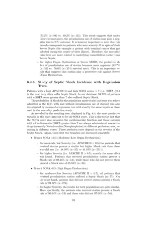
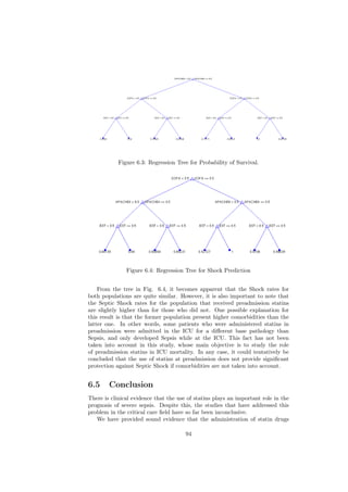
97. Chapter 7
Severe Sepsis Mortality
Prediction Using an
Interpretable Latent Data
Representation
No renuncio a nada, simplemente
hago lo que puedo para que las
cosas me renuncien a mi.
Julio Cortázar
7.1 Introduction
In this chapter, we propose the use of a latent model-based feature extraction
approach to obtain new sets of descriptors, or prognostic factors, for the predic-
tion of mortality due to Sepsis. The reported experimental results are readily
interpretable. Interpretation is, needless to say, a sensitive issue in the medical
ambit, and one that should not be underestimated: the lack of translation of
the prognostic factors into usable clinical knowledge would risk rendering the
proposed approach useless [107].
In the reported experiments, the obtained prognostic factors are used to pre-
dict mortality through standard logistic regression (LR), a method commonly
used in medical applications [108, 109] and widely trusted by clinicians. The
prediction accuracy results herein reported improve on those obtained with cur-
rent standard data descriptors and therefore provide support for the use of these
new factors as risk-of-death predictors in ICU environments.
7.2 Materials
As in previous chapters, this work resorts to a prospective observational cohort
study of adult patients with severe sepsis. The study was conducted at the
97

98. Critical Care Department of the Vall d’ Hebron University Hospital (Barcelona,
Spain), and it was approved by the Research Ethics Committee of the Hospital.
The database consists of data from patients with severe sepsis, collected at the
ICU by the Research Group in Shock, Organic Dysfunction and Resuscitation
(SODIR), between June, 2007 and December, 2010. During this period, 354
patients with severe sepsis (medical and surgical patients) were admitted in the
ICU.
The mean age of the patients in the database was 57.08 (with standard devi-
ation ±16.65) years; 40% of patients were female and the diagnosis on admission
was 56.15% medical and 44.85% surgical. The origin of primary infection for the
cases on the database was 40.24% pulmonary, 23.17% abdominal, 10.75% uri-
nary, 7.21% skin/muscle, 4.88% central nervous system (CNS), 1.55% catheter
related, 1.00% endovascular, 2.22% biliary, 4.99% mediastinum and 3.99% un-
known. The mortality rate for this extended dataset was 26.32%.
The collected data show the worst values for all variables during the first 24
hours of evolution for Severe Sepsis. Organ dysfunction was evaluated through
the SOFA score system [2], which objectively measures organ dysfunction for
6 organs/systems, the details of which are provided in Table 7.1. Severity was
evaluated by means of the APACHE II score (for further reference, see [1]). The
APACHE II score was 23.03 ± 9.62 for the population under study.
Table 7.1: List of SOFA scores, with their corresponding mean and standard
deviation values for the population under study (scoring organ dysfunction).
Cardiovascular (CV) 2.86 (1.62)
Respiratory (RESP) 2.31 (1.15)
Central Nerv. Sys. (CNS) 0.48 (1.00)
Hepatic (HEPA) 0.48 (0.92)
Renal (REN) 1.06 (1.20)
Haematologic (HAEMATO) 0.78 (1.14)
Global SOFA score 7.94 (3.86)
Dysf. Organs (SOFA 1-2) 1.68 (1.09)
Failure Organs (SOFA 3-4) 1.51 (1.02)
Total Dysf. Organs 3.18 (1.32)
The specific set of 34 features used for the mortality prediction analyses in
this chapter are listed in Table 7.2. Input data was scaled to have zero mean
and a standard deviation of 1.
7.3 Results
7.3.1 Diagnosis of the Factor Analysis Model
Given that the variables of the model do not follow a Gaussian distribution,
we proceeded to test if Ω is loaded in its diagonal. After computation of the
covariance of the residual error matrix, we calculate the sum of the diagonal
98

99. Table 7.2: List of variables used in this study.
Variable Description
v1 Age
v2 Gender
v3 Sepsis Focus
v4 Germ Class
v5 Polimicrobial Infection
v6 Base Pathology
v7 Cardiovascular SOFA score
v8 Respiratory SOFA score
v9 CNS SOFA score
v10 Hepatic SOFA Score
v11 Renal SOFA Score
v12 haematologic SOFA Score
v13 Total SOFA Score
v14 Dysfunctional Organs for SOFA 1-2
v15 Dysfunctional Organs for SOFA 3-4
v16 Total Number of Dysfunctional Organs
v17 Mechanical Ventilation
v18 Oxygenation Index P aO2 /F iO2
v19 Vasoactive Drugs
v20 Platelet Count
v21 APACHE II Score
v22 Surviving Sepsis Campaign Bundles 6h
v23 Haemocultures 6h
v24 Antibiotics 6h
v25 Volume 6h
v26 O2 Central Venous Saturation 6h
v27 Haematocrit 6h
v28 Transfusions 6h
v29 Dobutamine 6h
v30 Surviving Sepsis Campaign Bundles 24h
v31 Glycaemia 24h
v32 PPlateau
v33 Worst Lactate
v34 O2 Central Venous Saturation
99

100. elements was compared to the off-diagonal ones, for i ∈ {1 . . . d}. Specifically,
the value of K so that
d
|ωii | ≥ K |ωij |
j=1,j=i
was calculated, turning out to be K = 17.46 for all ωii . Because the maximum
off-diagonal element is much lower than any of the diagonal elements, diagonal
dominance is clear and it can be assumed that all possible interactions between
variables are accounted by the matrix Λ with 14 factors. The number of factors
have been selected according to the likelihood ratio presented in [110], which
proposes to select the minimum number of factors that assymptotically give a
χ2 distribution.
7.3.2 Factor Interpretation from a Clinical Viewpoint
As described in the previous subsection 7.3.1, the application of FA resulted in
a consistent 14-factor model of the original data set. The cumulative proportion
of total (standardized) sample variance explained by this model was found to
be 83.27%.
Table 7.3 summarizes the matrix of loadings corresponding to the original
variables listed in Table 7.2. Taking into consideration the highest factor load-
ings (in absolute value) for every given variable, these factors were mapped into
different easily interpretable clinical descriptors, explained as follows:
• Factor 1: Related to cardiovascular function and, more specifically, to the
cardiovascular SOFA score and vasoactive drugs c.f. table 6.1.
• Factor 2: Corresponds to haematologic function (haematologic SOFA
score and platelet count).
• Factor 3: Corresponds to respiratory function, Respiratory SOFA score
and P aO2 /F iO2 ratio.
• Factor 4: Corresponds to the use of mechanical ventilation and PPlateau.
• Factor 5: Corresponds to the 24h SSC bundles and glycaemic indices.
• Factor 6: Related to the micro-organism producing the Sepsis and whether
this sepsis polimicrobial or not.
• Factor 7: Corresponds to renal function measured by the SOFA score and
total SOFA score.
• Factor 8: Corresponds to the administration of antibiotics and haemocul-
tures taken during the first 6h of ICU stay.
• Factor 9: Relates to the number of organs in dysfunction for a moderate
SOFA and the total number of organs in dysfunction.
• Factor 10: Related to the hepatic function measured by the SOFA score.
• Factor 11: Corresponds to the CNS function measured by the SOFA score
and the number of organs in dysfunction.
100

101. • Factor 12: Related to the loci of Sepsis and whether the infection is polymi-
crobial or not.
• Factor 13: Corresponds to the APACHE II score and worst lactate levels.
• Factor 14: Relates the total number of organs in dysfunction.
The factors obtained with this method are coherent with the SOFA score
as a description and measure of organ failure and dysfunction [2], combined
with the management guidelines defined by the Surviving Sepsis Campaign [7].
Therefore, it can be safely concluded that they are related to SOFA and the
actions taken to mitigate this organ deterioration.
This is a result of particular interest. One of the main challenges in mor-
tality prediction is that of producing flexible models that can robustly fit the
observed data without the need for unnecessary contextual assumptions, and in
the presence of subtle interactions between covariates. This happens because
standard medical indicator-based models typically rely on hand-crafted para-
metric solutions to get around the problem [111]. One clear example of this is
the categorization of the SOFA score prognostic indicators described in section
7.2. The obtained FA solution goes beyond this categorization while accounting
for covariate interactions.
As mentioned in the introduction, the capability to interpret results is paramount
in real clinical applications [107]. The reported FA not only complies with this
requirement: it also provides a parsimonious data representation that can be
used as a basis for mortality prediction related to the Sepsis pathology.
7.3.3 Mortality prediction using logistic regression over
14 factors
We now progress to the task of mortality prediction itself, using the obtained
14-factor FA solution as starting point. The performance of the model was
evaluated by 10-fold cross validation. Table 7.4 shows the coefficient estimates
β, Z-Scores and maximum and minimum values resulting from fitting a logistic
regression model to the 14 factors (inputs) and the outcome in the ICU (output)
and removing those factors yielding Z-Scores smaller than 1.96. The Z-Scores
measure the effect of removing one factor from the model [110, 81]. A Z-score
greater than 1.96 in absolute value is significant at the 5% level and provides a
measure of the relevance for the prediction of a given factor.
As shown in table 7.4, factor 3, which is related to Mechanical Ventilation
and Pplateau, shows the strongest effect together with factor 13, which is related
to the APACHE II score. Factor 8 (Hepatic Function measured with the SOFA
Score) and factor 10 (related to the number of Dysfunctional Organs) are also
found to be relevant. It is worth noting at this stage that, with LR, the factors
related to the Surviving Sepsis Campaign show no strong effect on mortality
prediction. This result may be due to the low compliance with the Surviving
Sepsis Campaign Bundles for the first 6 and 24 hours of evolution (26.18 % and
44.06 % respectively for the ICU under study). However, it is interesting to note
that factor 9 (antibiotic administration and haemocultures) presents a higher
impact than that of factor 6 (24 h. bundles with glycaemic indexes). For our
ICU, 80.22 % of patients received antibiotics during the first 6 h of evolution
and 77.14 % had haemocultures during the same period of time. In fact, timely
101

102. Table 7.3: Loadings Matrix: |Λ(i, j)| > quantile 95 for Factor fi are presented
in bold.
F1 F2 F3 F4 F5 F6 F7 F8 F9 F10 F11 F12 F13 F14
v1 .27 -.12 -.05 .03 -.11 -.05 .08 -.04 .10 -.03 .08 -.16 .22 -.09
v2 .00 .02 .14 .13 -.13 .04 .21 .02 .03 -.01 -.09 -.09 -.04 -.04
v3 .13 .06 -.32 -.07 .00 .06 .01 -.04 .08 .19 .07 .42 -.08 .06
v4 -.12 -.03 -.01 .06 -.8 .98 -.04 -.03 -.03 -.05 -.04 -.03 -.03 -.04
v5 -.01 .05 -.01 .04 .05 .70 .04 -.07 -.02 -.01 -.02 .09 -.04 .03
v6 .16 -.21 .23 .13 .05 .06 -.02 -.05 .05 -.03 -.07 .47 .03 .13
v7 .97 .09 -.03 .15 -.01 -.03 .09 -.01 .02 .04 .01 .02 .07 .01
v8 .08 .03 .86 .38 -.01 .01 .05 .05 -.05 .12 .06 -.02 -.10 .09
v9 .11 -.01 .00 .09 -.06 -.05 .01 .03 .06 .05 .95 -.02 .05 -.01
v10 .13 .18 .07 .00 .12 -.04 .10 -.01 .14 .94 .05 .08 .04 -.01
v11 .20 .14 -.04 -.01 -.03 .01 .89 -.06 .10 .05 .02 .04 .09 .05
v12 .14 .97 .04 .05 .03 .02 .04 .00 .04 .10 .02 .10 .07 -.05
v13 .61 .37 .27 .20 .03 -.01 .43 -.01 .11 .32 .26 .09 .01 -.06
v14 .01 .23 -.05 -.11 .03 -.06 .11 .04 .94 .13 .07 .09 .04 -.01
v15 .56 .33 .24 .28 -.02 -.02 .31 .01 -.36 .23 .28 .04 .08 .26
v16 .44 .44 .15 .12 .02 -.06 .33 .04 .48 .30 .28 .09 .11 .21
v17 .18 .07 .13 .95 -.04 .03 .08 .05 -.06 .06 .11 -.05 .01 .02
v18 .05 -.10 .82 .04 .04 .02 -.03 -.08 -.01 -.03 .02 .17 .06 .04
v19 .92 .12 -.06 .13 -.02 .08 .08 .02 -.01 .03 .01 .03 .02 .04
v20 -.08 -.63 -.03 .00 -.01 .01 -.16 .04 -.18 -.03 -.02 .04 .00 -.08
v21 .38 .17 .25 .36 -.09 .03 .40 .04 .05 .09 .23 .05 .46 -.06
v22 -.11 -.02 .15 .01 .03 .08 .00 .52 .09 -.01 .08 .08 .10 -.07
v23 .16 .04 .03 -.07 .02 -.08 .01 .69 -.05 .05 .06 -.12 -.06 .02
v24 .01 -.03 -.02 .00 .04 -.10 -.03 .62 .01 -.01 -.07 -.11 .02 .02
v25 .46 .07 -.04 .10 .10 .05 -.02 .34 .01 -.03 -.02 .04 .21 -.03
v26 -.10 -.01 -.02 -.07 -.11 -.04 -.05 .05 .07 .11 .11 .09 .04 .01
v27 .04 -.10 -.02 .00 .05 -.03 -.02 .22 -.01 -.01 .00 -.41 -.09 .08
v28 -.05 .06 .02 -.08 .00 -.05 -.04 .04 .01 .07 .05 -.02 -.01 -.06
v29 .09 .24 .03 .18 .06 .06 -.02 .04 -.01 .07 -.01 -.06 .06 .12
v30 .00 .05 -.04 -.09 .90 -.07 -.01 .08 -.01 .05 -.01 .01 .02 -.02
v31 .01 -.05 -.01 .01 -.10 .98 .02 .05 .07 .09 -.01 -.01 -.03 -.10
v32 -.15 -.06 -.18 -.54 .12 -.04 -.01 .09 .05 .08 .00 -.09 -.05 .01
v33 .28 .20 .11 .21 .04 -.03 .24 .08 -.04 .19 -.03 .14 .31 .04
v34 .21 .11 -.07 -.02 .04 .07 .00 .24 .05 .02 .04 .03 .31 .03
102

103. administration of antibiotics and performance of haemocultures are considered
critical to improving the prognosis of septic patients.
Regression on the 14 factors together with 10-Fold cross validation resulted
in an AUC of 0.78. A decision threshold of γ = 0.68 was automatically selected
(for the maximization of the discrimination probability) to decide whether the
patient survives. This 10-fold cross-validation experiment yielded an AUC of
0.78, an error rate of 0.24, a sensitivity of 0.65 and a specificity of 0.80. The
results of LR over latent factors is presented in table 7.4. This table also shows
that the two most representative factors are F10 and F13, which correspond
to organ dysfunction measured through the SOFA score and illness severity
measured through the APACHE II score combined with the worst lactate levels.
Table 7.4: Results for LR over Latent Factors with 10-fold cross validation
β Coeff MAX MIN Z-score
Intercept 1.22 1.53 .87 7.11
F4 -0.54 -0.23 -0.86 -3.38
F10 -0.69 -0.38 -1.05 -4.26
F9 -0.51 -0.21 -0.81 -3.36
F13 -0.49 -0.24 -0.74 -3.80
7.3.4 Comparison with Logistic Regression over a Selec-
tion of the Original Variables
Further experiments aimed to compare the predictive ability of the FA 14-factor
solution with that of the original data attributes were carried out. For that, the
most significant clinical attributes were selected in a backward feature selection
process (in our case, the backward feature selection removes those variables
resulting in non-significative Z-scores). The selected attributes were: the total
number of dysfunctional organs; the APACHE II score; and the worst lactate
levels. The corresponding coefficients, maximum and minimum values and Z-
scores for these three variables are presented in table 7.5.
Table 7.5: Results for LR with 10-fold cross validation
β Coeff MAX MIN Z-score
Intercept 4.20 3.11 5.29 7.56
APACHE II -0.08 -0.13 -0.04 -3.77
Worts Lact. -0.25 -0.38 -0.11 -3.63
Regression on the most significant attributes together with 10-fold cross
validation yield an AUC of 0.75, a lower result than the one obtained with
the FA solution. Following the procedure outlined in the previous subsection,
a decision threshold of γ = 0.68 was automatically selected. This resulted in
a prediction error over the test data of 0.3 (higher than the FA solution), a
specificity of 0.72, and a sensitivity of 0.64.
103

104. 7.3.5 Comparison with the APACHE II Mortality Score
The Risk-of-Death (ROD) formula based on the APACHE II score can be ex-
pressed as [1]:
ROD
ln = −3.517 + 0.146 · A + (7.1)
1 − ROD
Where A is the APACHE II score and is a correction factor depending on
clinical traits at admission in the ICU. For instance, if the patient has undergone
post-emergency surgery, is set to 0.613. The application of this formula with
a threshold of γ = −0.25 to the population under study yields an error rate of
0.28 (higher than the FA solution), a sensitivity of 0.82 and a specificity of 0.55.
The AUC was 0.70.
A previous study [112] presented very similar results to those reported in this
section for a similar ICU. Furthermore, a recent study from 2009 [113] presented
very similar results to those reported here for neurocritically ill patients (with
a very low sensitivity of 0.47).
7.4 Conclusions
Sepsis is a prevalent pathology in the clinical ICU environment, and one as-
sociated with relatively high levels of mortality. Its medical management is
therefore both a sensitive issue and a serious challenge to health care systems.
The clinical indicators of Sepsis currently in use are known to be of limited
relevance as mortality predictors. In the assessment of ROD for critically ill
patients, sensitivity is important due to the fact that more aggressive treatment
and therapeutic actions may result in better outcomes for high risk patients.
As validated by the results reported in section 7.3.5 and similar ones reported
in other studies [112], the ROD formula presented in [1] is very sensitive but
also quite poor in terms of specificity (i.e., it results in a high number of false
negative cases). This is despite the fact that it is widely accepted in practice
and yields acceptable accuracy results. Its poor specificity may be the result of
its formula being based on clinical traits and the APACHE II score only.
In this chapter, we have put forward a new and simple method for the as-
sessment of ROD in septic patients. It proposes a change of data representation
in the form of feature extraction using FA, and uses LR over the resulting latent
factors for the prediction itself. The main advantage of the proposed approach is
that it removes collinearities and noisy inputs while keeping the method simple
and fully interpretable from a clinical point of view. In other words, the strength
of this study lies in the fact that it is possible to derive a prognostic score from
a set of physiopathologic and therapeutic variables, which are available at the
onset of Severe Sepsis.
Although one might well object that it is easier to assess three variables
than three factors (i.e. LR against Factor Analysis), we must stress the fact
that the three factors obtained are actionable at ICU admittance whilst the
worst lactate, which is the most predictive variable for LR is time consuming
and may not take place at ICU admittance.
The proposed method may be understood as a generalization of the ROD for-
mula introduced in [1], where the corrective factor, which models clinical traits
at admittance in the ICU, is accounted for by the latent-factor representation.
104

105. It takes not only the contribution of the APACHE II score into consideration,
but also other important clinical traits such as the number of dysfunctional or-
gans combined with the Sequential Organ Failure Assessment (SOFA), which
also impacts on the mortality rates of Septic patients. The reported ROD as-
sessment takes into consideration the Respiratory and Hepatic SOFA scores. It
is precisely all the extra parameters considered in our experiments the reason
behind the significant improvement on specificity if compared with the original
specificity of the APACHE II score (i.e. 0.55). This improvement is achieved
while keeping model complexity under control and without compromising the
interpretation of the results (given that all the parameters involved are routinely
monitored in an ICU).
A word of caution must be given, though, as the system performance has
only been evaluated in a single ICU and limited population samples. For this
reason, future work should lead toward a multi-centric prospective study, in
order to validate the generalizability of the method.
105

106. 106

107. Chapter 8
Severe Sepsis Mortality
Prediction from Observed
Data
You know my methods. Apply
them.
Sherlock Holmes
8.1 Introduction
So far we have focused on the study of dependence relations between the dif-
ferent variables and clinical traits and exploited its marginalisation to study
the incidence of Severe Sepsis or its prognosis by means of Factor Analysis and
Logistic Regression. We have been working on already interpretable indicators
that could be used by the clinical practice.
In this approach we first embed the data in a suitable feature space, and then
use algorithms based on linear algebra, geometry and statistics for inference.
With this informal definition, it becomes apparent that all the methods used
so far could be kernelized as long as we used the appropriate mappings, spaces,
measures and topologies. Given the simplicity of the models used in this PhD
(i.e. we only have multinomial and multivariate Gaussian distributions, which
can be efficiently modelled algebraically by means of the Regular Exponential
Family) we propose to use a generative approach and exploit the inner structure
of our data in order to build a set of efficient closed-form kernels best suited for
these two distributions (see sections 4.6 and 4.6.2).
For the experiments in this chapter, the database of patients of chapter 7
was available. It was used to investigate the performance of RVM and Gen-
erative Kernels as an ICU Sepsis Mortality Predictor. This performance was
then compared to that of alternative techniques currently in use for ICU-related
prediction, such as shrinkage methods for logistic regression and a risk-of-death
(ROD) formula based on the standard APACHE II score [1]. The proposed mod-
els are shown to outperform these techniques, while simultaneously assessing the
107

108. relative impact of individual indicators of the pathology on the prediction.
Interestingly, a number of these indicators, which are also readily inter-
pretable, are shown to have an impact on mortality prediction. We believe that
this is a result that should help to simplify the decision making process at ICU.
This chapter uses the same dataset presented in chapter 7.
8.2 Materials: Detailed Description of Genera-
tive Kernels
In this section we present two of the main contributions of this PhD thesis:
the Quotient Basis Kernel (QBK) and the simplified Fisher kernel. The meth-
ods presented in this section will be tested in the context of dimensionality
reduction presented in chapter 5: RVM, the Lasso, ridge regression and logistic
regression with backward feature selection. The set of attributes selected from
these methods is later used with the kernels presented in this section.
8.2.1 Quotient Basis Kernel
In this section we use the definitions of algebraic models as presented in chap-
ter 4. Inputs are denoted by x, responses or outputs are denoted by y as in
chapter 5, parametric functions are denoted by η or functions of η. These are
related by polynomial algebraic relations, possibly implicit (cf. section 4.2).
Another feature of this definition is that constraints of polynomial type can be
included in the specification of the model. Implicit models and the introduction
of constraints can lead to the use of dummy variables.
The parameters of the model as interpreted in statistics are functions of any
form with the restriction that they belong to a specified field. For example,
Q (η1 , . . . , ηp ) is the set of all rational functions in η1 , . . . , ηp with rational co-
efficients. Another example is Q eη , . . . , eη the set of all exponential rational
1 p
functions. Parameters are treated as unknown quantities and in most cases ap-
pear in linear form. The algebraic space used is the commutative ring of all
polynomials K[x1 , . . . , xs ] in the indeterminates x1 , . . . , xs and with coefficients
in the field K (in our case R).
For a given initial ordering, a term is specified by the vector of length s of
its exponents. Therefore Term{s} is coded by Zs [57] (set of positive integers).
+
When the indeterminates are indexed from 1 to s so that x1 , . . . , xs , it is
convention to consider an initial ordering xi xi+1 ∀i = 1 . . . s − 1.
Definition 42. Polynomial Ideal (c.f. definition 12):
1. A polynomial ideal I is a subset of a polynomial ring K[x] closed under
sum and product by elements of K[x]. Specifically the set I ⊂ K is an ideal
if ∀f, g ∈ I and s ∈ K the polynomials f + g and sf are in I.
2. Let F be a set of polynomials. The ideal generated by F is the smallest
ideal containing F . It is denoted F .
3. An ideal I is radical if f ∈ I whenever a positive integer m exists such
that f m ∈ I.
√
4. The radical of an ideal I is the radical ideal defined as I = {f ∈ K : ∃m|f m ∈ I}
108

109. The Hilbert basis theorem ([57]) shows that every ideal has a finite basis.
This provides a very powerful result since it means that any ideal is finitely
generated (even if the generating set is not necessarily unique). Another power-
ful result is that this generation basis is of a special type called Gröbner Basis,
which we define below. This bases will become essential in the derivation of
regression/interpolation polynomials and also for the algebraic derivation of the
Fisher and the proposed QBK kernels.
Definition 43. [57] (c.f. definition 6) Let τ be a term ordering on K[x] and f
a polynomial in K[x]. The leading term of f , LTτ (f ) is the largest term with
respect to τ among the terms in f .
Definition 44. [57] Gröbner Basis (c.f. definition 14): Let τ be a term ordering
on K[x]. A subset G = g1 , . . . , gt of an ideal I is a Gröbner basis of I with respect
to τ iff
LTτ (g1 ), . . . , LTτ (gt ) = LTτ (I) (8.1)
where LTτ (I) = {LTτ (f ) : f ∈ I}.
Theorem 15. [63, 57] (c.f. theorem 4) Given a term ordering, every ideal I
except {0} has a Gröbner basis and any Gröbner basis is a basis of I.
Definition 45. Gröbner basis of unique points [63, 57] (c.f. section 4.2.3): Let
A be a set of n unique points A = {a1 , . . . , an } and τ a term ordering. These
points can be presented as the set of solutions of

 g1 (a) = 0

g2 (a) = 0

(8.2)

 ···
gt (a) = 0

Where G = g1 , . . . , gt is a Gröbner basis of A.
Let us formally define the Quotient Basis ESTτ that shall be used in the
algorithm below.
Definition 46. [57] Quotient Basis (c.f. definition 15):
Let A be a set of unique support points A = {a1 , . . . , an } and τ a term
ordering. A monomial basis of the set of polynomial functions over A is
ESTτ = {xα : xα ∈ LT(g) : g ∈ I(A) }
/ (8.3)
This definition states that ESTτ comprises the elements xα that are not
divisible by any of the leading terms of the elements of the Gröbner basis of
I(A).
Theorem 16. [57] (c.f. theorem 5) The set ESTτ has as many elements as
there are support points.
Definition 47. Design Matrix 35 (c.f. definition 35)
Let τ be a term ordering and let us consider an ordering over the support
points A = {a1 , . . . , an }. Let L be the set of exponents of ESTτ . We call design
matrix the following matrix
Z = [aα ]i=1,...,N,α∈L
i (8.4)
109

110. Theorem 17. [57] (c.f. theorem 14)
1. Z is non-singular.
2. Let ei be the d dimensional canonical vector (i.e. with components 0 except
in position i where it has value 1. For all i = 1, . . . , d there exists a vector
ci such that
Z · c(i) = ei
and the polynomial α∈L ciα xα interpolates the indicator function of the
support point ai . That is
1 x = ai
ciα xα =
0 x = ai and x ∈ A
α∈L
Proposition 8. (c.f. proposition 3) The covariance of Z,
cov(Z) = E Z − E(Z))(Z − E(Z))t
is a kernel.
Definition 48. Quotient Basis Kernel (QBK) (c.f. corollary 1):
The covariance of the design matrix of ESTτ , which is a kernel, is the QBK.
The algorithm for the calculation of ESTτ , which shall be used to calculate
our QBK from the design matrix Z is described in algorithm 1. This algorithm
was originally developed for the derivation of interpolation/regression polyno-
mials in [63].
Algorithm 1 Pseudocode for the Quotient Basis Kernel
Input: x and y and ESTτ
Output: Quotient Basis Kernel k(x, y)
µx ← mean(x)
µy ← mean(y)
Zx ← [xα ]i=1,...,N,α∈L {Subs. x in the design matrix calculated from ESTτ }
i
α
Zy ← [yi ]i=1,...,N,α∈L {Subs. y in the design matrix calculated from ESTτ }
t
k(x, y) ← (Zx − µx ) (Zy − µy )
8.2.2 Fisher Kernel for Exponential Families
Lets us recall from section 4.6.2 that the computation of the Fisher Kernel is
computationally expensive. Therefore, we propose to use the simplified (prac-
tical) Fisher Kernel from the sufficient statistics (T ) as defined below:
Definition 49. Practical Fisher Kernel
¯ ¯
k(x, z) = U (Tx , η)U (Tz , η)t (8.5)
Where Tx and Tz are the sufficient statistics estimated on x and z.
¯
Here U (Tx , η) is the score function as defined in section 4.6.2. The product
of distances of each point can be understood as a further simplification of the
method presented in [114], which approximates distances between gradients (see
section 4.6) through a stochastic selection rule.
110

111. Algorithm 2 Pseudocode of the Practical Fisher Kernel for Multinomial Dis-
tributions
Input: X and Z
Output: Fisher Kernel k(X, Z)
µX ← mean(X)
µZ ← mean(Z)
for i = 1 · · · NX do
for j = 1 · · · NZ do
t
k(i, j) ← (TXi − µX ) TZj − µZ
{Prod of distances of each point to their mean}
end for
end for
8.2.3 Kernels based on the Jensen-Shannon metric
The Kernels based on the Jensen-Shannon metric have been formally presented
in section 4.6.3. For the sake of clarity, here we give a short overview about the
propositions that yield these generative kernels.
Definition 50. [76, 77, 78]
Let γ1 , γ2 ∈ M (parameters in dual space) and F the dual of the cummuluant
generating function G, by definitions 39, 40 and A.10:
F (γ1 ) + F (γ2 ) γ1 + γ2
JS(γ1 , γ2 ) = −F . (8.6)
2 2
Proposition 9. [76, 77, 78] Centred Kernel
By property 8 and definition 40, let x0 ∈ X define the centred kernel as
φ:X ×X →R
φ(x, y) = JS(x, x0 ) + JS(y, x0 ) − JS(x, y) − JS(x0 , x0 ). (8.7)
Proposition 10. [76, 77, 78] Exponentiated Kernel
By property 9 and definition 40, we define the exponentiated kernel as φ :
X ×X →R
φ(x, y) = exp(−tJS(x, y)) (8.8)
∀t > 0.
Proposition 11. [76, 77, 78] Inverse Kernel
By proposition 10 and definition 40, we define the exponentiated kernel as
φ:X ×X →R
1
φ(x, y) = (8.9)
t + JS(x, y)
∀t > 0.
It is obvious that the most important part to calculate the kernels outlined
above is the calculation of the Jensen-Shannon metric in dual-space. The pseu-
docode to implement this metric is given in algorithm 3.
111

112. Algorithm 3 Pseudocode to the Jensen-Shannon Metric for Multinomial Dis-
tributions
Input: X and Z
Output: Dual JS(γi , γj )
for i = 1 · · · NX do
for j = 1 · · · NZ do
γ1 ← X(i, :)
γ2 ← Z(j, :)
{Compute F}
{Compute JS from Duals}
F (γi )+F (γj ) γ +γ
JS(γi , γj ) ← 2 −F i2 j
end for
end for
Algorithm 4 Pseudocode to Compute Duals for Multinomial Distributions
Input: Vector γx
Output: Dual F (γx )
N= γx
F ← γx log( γx )
N
8.3 Results
8.3.1 Mortality Prediction with RVM
The model performance was evaluated by means of 10-fold cross-validation. The
RVM yielded an accuracy of mortality prediction of 0.86 as measured by the area
under the ROC plot (AUC); a prediction error of 0.18; a sensitivity (proportion
of correctly predicted survivors out of all survivors) of 0.67; and a specificity
(proportion of correctly predicted exitus out of all exitus) of 0.87.
Beyond classification accuracy, and as described in the previous section,
RVM performs soft feature selection through automatic feature relevance deter-
mination. The following relevance vector (with the weights associated to each
input feature) was obtained:
• Number of dysfunctional organs (w1 = −0.039)
• Mechanical Ventilation (w2 = −0.101)
• APACHE II (w3 = −0.337)
• Resuscitation Bundles (6h) (w4 = 0.037)
The coefficients corresponding to the rest of features were set by RVM to
zero (i.e. lower than the numeric tolerance set in Matlab: 2.2 × 10−16 ) as part
of the training process. This effectively reduces the complexity of the predic-
tion procedure (34 features reduced down to just 4) and consequently, improves
its interpretation. Given that a linear basis function was used to estimate the
relevance vector, it becomes apparent that the negative weights (number of dys-
functional organs, mechanical ventilation, APACHE II) are related to a higher
mortality risk (note again that we have coded survival as 1 and exitus as -1),
112

113. whereas the SSC bundles (resuscitation bundles) are associated to a protective
effect (i.e. antibiotics administration, performance of haemocultures, adminis-
tration of volume and vasoactive drugs and so on). In fact, timely administration
of antibiotics and performance of haemocultures are considered critical to im-
proving the prognosis of septic patients. Equally important is the knowledge of
which features are deemed not to be relevant by RVM.
The set of variables selected by the RVM also present clinical relevance since
they are widely used in clinical practice for the assessment of ROD [1, 25, 7]. Of
particular interest are the SSC bundles due to the relevant scientific information
supporting them [7]. It is this subset of variables selected by the RVM
that shall be used in the next sections of this chapter.
8.3.2 Comparison with Shrinkage Feature Selection Meth-
ods for Logistic Regression
The predictive ability of the RVM was then compared to that of other well es-
tablished shrinkage methods for logistic regression. In particular, we have tested
the performance against Ridge Regression, the Lasso and Logistic Regression.
The latter using a subset of features selected in a backward process by remov-
ing those coefficient yielding the lowest Z-scores [81]. The selected features and
coefficients for each method were:
• Ridge Regression:
– Number of dysfunctional organs for SOFA 3-4 (w1 = −0.021)
– APACHE II (w2 = −0.127)
– Worst Lactate (w3 = −0.126).
• Lasso:
– Age (w1 = 0.007)
– Germ Class (w2 = 0.005)
– P aO2 /F iO2 (w3 = 0.001)
– APACHE II (w4 = −0.006)
– SvcO2 6h (w5 = −0.001)
– Haematocrit 6h (w6 = 0.009)
– Worst Lactate (w7 = −0.023)
– SvcO2 (w8 = −0.006).
• Logistic Regression with backward feature selection:
– Intercept (w1 = 4.20)
– Number of Dysfunctional Organs (w1 = −0.12)
– APACHE II (w2 = −0.08)
– Worst Lactate (w3 = −0.25)
113

114. The three shrinkage methods evaluated in this section agreed in detecting as
prognostic factors the Severity measured by the APACHE II score and acido-
sis measured by the lactate levels. Apart from that, it becomes apparent that
organ dysfunction and mechanical ventilation or other parameters related to it
like P aO2 /F iO2 also play a role in the prognosis of Sepsis. Table 8.1 shows the
results of AUC, error rate, sensitivity and specificity for each method. So far
we have tested different approaches to the study of the prognosis of sepsis rang-
ing from dimensionality reduction algorithms like Factor Analysis to Shrinkage
Methods like Ridge Regression and the Lasso. In this section we have shown
that application of the RVM outperforms all the methods outlined so far in
terms of AUC and specificity.
Table 8.1: Results for Shrinkage Methods
Method AUC Error Rate Sens. Spec.
RVM 0.86 0.18 0.67 0.87
Logistic 0.75 0.30 0.64 0.72
Ridge 0.70 0.25 0.63 0.79
Lasso 0.70 0.32 0.67 0.68
8.3.3 Mortality Prediction with Generative Kernels
The different kernels have been implemented in Matlab following the algorithms
and propositions outlined above.
The calculation of the Quotient Basis Kernel required the implementation of
the algorithm outlined above to calculate ESTτ with the lexicographic ordering.
The input to algorithm were the unique points of our input data for each
of the four variables of interest selected by the RVM (i.e. all the observed
combination of points from the input) 1 . Here
• x1 is the Number of Dysfunctional Organs as measured by the SOFA
Score.
• x2 corresponds to Mechanical Ventilation (yes/no).
• x3 corresponds to Severity as Measured by the APACHE II Score.
• x4 corresponds to the SSC Resuscitation Bundles (i.e. administration of
antibiotics, performance of haemocultures and so on). This is also a binary
variable.
The resulting Quotient Basis ESTτ for our dataset is
1 The rationale behind selecting this subset is that not only has been automatically gen-
erated but is also in good agreement with common clinical practice since it balances organ
dysfunction with timely administration of antibiotics
114

115.  

 1, x4 , x3 , x3 x4 , 

x2 , x2 x4 , x2 x3 , x2 x3 x4 ,

 


 

x2 , x2 x4 , x2 x3 , x2 x3 x4 ,

 


 2 2 2 2 

x3 , x3 x4 , x3 x3 , x3 x3 x4 ,

 


 2 2 2 2 

x4 , x4 x4 , x4 x3 , x4 x3 x4 ,

 

 2 2 2 2 
ESTτ = x5 , x5 x4 , x6 , x1 ,
2 2 2
x1 x4 , x1 x3 , x1 x3 x4 , x1 x2 ,

 


 

x1 x2 x4 , x1 x2 x3 , x1 x2 x3 x4 , x1 x2 ,

 


 2 

x1 x2 x4 , x1 x2 x3 , x1 x2 x3 x4 , x1 x3 ,

 


 2 2 2 2 

x1 x3 x4 , x1 x3 x3 , x1 x3 x3 x4 , x1 x4 ,

 


 2 2 2 2 

x1 x4 x4 , x1 x4 x3 , x1 x5
 
2 2 2
The Quotient Basis Kernel is calculated by taking the Covariance after trans-
forming the input points with ESTτ . Regarding interpolation, our sample space
has 2016 unique points (i.e. 7 × 2 × 72 × 2 corresponding to the possible number
of dysfunctional organs, mechanical ventilation, APACHE II and SSC resusci-
tation bundles). In our database, we have 354 different patients with a 7.63%
repeated samples (i.e. 327 unique independent points). This means that we
only have 16.22% of the available sample set.
At this stage, it is important to note that this Quotient Basis accounts for
all the interactions between the different input variables. From section 4.4.2,
this would mean that the four variables are conditionally dependent and also
that this data can be represented by means of a fully connected graph. This
interpretation is consistent with standard clinical practice.
Besides that, we have used Matlab’s Support Vector Machine QP solver
implemented in the BioInformatics and Optimization Toolboxes. We have also
used 10-fold cross validation to evaluate the classification performance for the
different kernels and also compare with the results presented in other chapters
of this PhD Thesis. A grid search yielded the appropriate values for C (c.f.
section 5.2.2) parameters for each Kernel. More particularly,
• Quotient Basis and Fisher C = 1.
• Generative Kernels C = 10. Also the parameter t for the Exponential and
Inverse Kernels was set to 2.
• Gaussian, Linear and Polynomial Kernels C = 10.
Statistical significance between errors has been tested by means of the Wilcoxon
Rank Sum Test. The null hypotheses that we tested is whether the the errors
are independent samples from identical continuous distributions with
equal medians [115]. This test accepted the null hypothesis in all cases; the
p-values for this test are given in table 8.3. Of course, the level of agreement
measured by the p-value differs between the different kernels.
From table 8.2, it becomes apparent that there is no significant difference
in performance between the most widely used kernels (Gaussian/Multivariate,
Polynomial and Linear) as opposed to the four Generative Kernels tested. More-
over, all generative kernels yielded a good balance between AUC, sensitivity and
specificity. However, from our results, it is also apparent that the Fisher ker-
nel and the Quotient Basis kernel yield the best results (i.e. best error rate,
AUC and balance between sensitivity and specificity). Table 8.2 also shows the
115

116. average time taken to compute each kernel and train the SVM for the given
dataset.
Table 8.2: Results for SVM with Generative Kernels
Kernel AUC Error Rate Sens. Spec. CPU time [s]
Quotient 0.89 0.18 0.70 0.86 1.45
Fisher 0.76 0.18 0.68 0.86 1.39
Exponential 0.75 0.21 0.70 0.82 1.64
Inverse 0.62 0.22 0.70 0.82 1.68
Centred 0.75 0.21 0.70 0.82 1.99
Gaussian 0.83 0.24 0.65 0.81 1.56
Poly (order 2) 0.69 0.28 0.71 0.76 1.59
Linear 0.62 0.26 0.62 0.78 1.35
Table 8.3: p-value table for the Wilcoxon Rank Sum Test. The null hypothesis
tested is that the cdf for the resulting error distributions for each kernel are
different
Quotient Fisher Exp Inv Cent Gauss Lin Poly
Quotient X 0.91 0.78 0.70 0.57 0.30 0.57 0.52
Fisher X 0.82 0.60 0.42 0.91 0.60 0.67
Exp X 0.49 0.35 0.83 0.30 0.52
Inv X 0.51 0.47 0.67 0.38
Cent X 0.42 0.27 0.17
Gauss X 0.41 0.67
Lin X 0.41
Poly X
8.4 Conclusions
In the assessment of ROD for critically ill patients, sensitivity is important due
to the fact that more aggressive treatment and therapeutic actions may result
in better outcomes for high risk patients. As validated by the results reported in
section 7.3.5 and similar ones reported in other studies [112], the ROD formula
presented in [1] is poor in terms of sensitivity (i.e., it results in a high number of
false negative cases). This is despite the fact that APACHE is widely accepted
in practice and yields acceptable accuracy results. Its poor sensitivity may be
the result of its formula being based on non-sepsis specific clinical traits and the
APACHE II score only.
In this chapter, we have put forward an RVM-based method for the predic-
tion of ROD in septic patients. It has been shown to produce accurate results,
116

117. particularly in terms of specificity, while improving the interpretation and ac-
tionability of the results through an embedded feature relevance determination
process. This method has proven to be superior in terms of accuracy (error rate,
specificity and AUC) than other well established shrinkage methods (Lasso and
Ridge). Specifically from a medical viewpoint, the strength of this study lies
in the fact that it shows that it is possible to derive a reliable prognostic score
from a parsimonious set of physiopathologic and therapeutic variables, which
are available at the onset of severe sepsis for medical experts at the ICU.
The SVMs have been trained with eight different kernels out of which five
were generative and the other three are kernels considered well suited for the
problem at hand. Regarding the generative kernels, one is completely new (i.e.
the Quotient Basis kernel) while the Fisher kernel has been derived by means
of a combination of Algebraic Models and well established properties from the
Regular Exponential Families.
The kernels proposed have proven to provide accurate and actionable results
whilst keeping an acceptable balance between the different parameters of interest
(AUC, error rate, sensitivity and specificity). In particular, the newly proposed
Quotient Basis Kernel provided the most accurate results and almost equivalent
to those of the the Fisher kernel in terms of balance between sensitivity and
specificity (i.e. good proportion between positives and negatives). However, a
Wilcoxon rank sum shows that all results are statistically equivalent.
The proposed methods may be understood as a generalization of the ROD
formula introduced in [1], where the corrective factor, which models clinical
traits at admittance in the ICU. The indicators obtained not only take the
contribution of the APACHE II score into consideration, but also other impor-
tant life-threatening clinical traits such as the number of dysfunctional organs
combined with mechanical ventilation (RVM) or worst lactate levels (shrinkage
methods). The prognosis indicator is also balanced with important procedures
to overcome sepsis such as the administration of volume, antibiotics, vasoactive
drugs and the performance of haemocultures (i.e. SSC resuscitation bundles).
117

118. 118

119. Chapter 9
Conclusions
Good reasons must, of force, give
place to better.
William Shakespeare
In the previous chapters, we have first defined the general problem of Sepsis
data analysis in the ICU environment and we have then focused our attention on
some of the main challenges it involves, including the estimation of the incidence
of sepsis, the prediction of ICU outcome for patients with Severe Sepsis and
the impact of the pre-administration of statin drugs on such outcomes. To
address these problems, we employed a wide array of techniques from the fields
of multivariate and algebraic statistics, algebraic geometry, machine learning
and computational intelligence. More specifically, ASMs have set the basis for
the estimation within the geographic ambit of the study of the incidence of
Sepsis. This has been accomplished using the Hammersley-Clifford theorem,
which has enabled us to study this incidence as a hidden variable in a Bayes
Network.
One of the main limitations of the quantitative methods for the assessment
of Risk of Death currently in use at the ICU is their lack of specificity (i.e. the
high number of false positive cases they incur), which not only puts an extra
risk on an already severely affected patient population, but also results in an
unnecessary burden for National Health Systems. In this regard, it has been
shown that Machine Learning and related techniques can play an important
role as they improve the overall performance by combining those indicators
already in place with other clinical variables, which are routinely measured (even
if not commonly used as indicators) such as the Surviving Sepsis Campaign
Resuscitation Bundles (i.e. timely administration of antibiotics, performance of
haemocultures and volume administration if necessary).
In this thesis this problem of ICU outcome prediction has been addressed
according to two general approaches. The first involved a transformation of the
originally observed data variables into new hidden or latent features that can
be interpreted in medical terms and thus be used as new clinical indicators.
The second involved using the original measurements in analyses that applied
several strategies involving classification and dimensionality reduction. They
included the use of classifiers such as logistic regression (common practice in
119

120. the medical field), SVMs and RVMs. The latter related to techniques of feature
selection (Ridge Regression or the Lasso) that have also been used with some of
the classifiers. Even if different feature selection methods resulted in different
subsets of selected variables, all of them pointed towards the same physiological
systems (for example acidosis or mechanical ventilation parameters) and organ
dysfunctions.
Attending to the nature of the indicators and clinical traits used in the
medical practice, we have further built upon the ASM by relating them to the
Regular Exponential Family. This can be intuitively understood as the means to
re-parametrize a given support and under a given family (the multinomial dis-
tribution is also a Regular Exponential Family), in order to obtain a convex dual
that simplifies the kernel generation. Another important result that we used is
that this convex-dual is the Entropy Function (for the multinomial family this
it is related to the relative frequencies), which can be calculated more efficiently.
We have also used the ASM methodology to derive a new kernel (Quotient Basis
Kernel), that is closely related to the Graphical Models presented in this PhD
Thesis.
9.1 On the Incidence of Sepsis and Coadjutant
Factors to be Taken into Consideration
Since its inception, the SIRS pathology has proven to be a sensitive indicator
of Sepsis [43], but also one of poor specificity. For example, Pittet et al. [44]
presented a SIRS incidence of up to 93% in critical care patients, while Rangel et
al. have shown an incidence of 68% [43]. The latter study also shows that 25%
of patients with SIRS developed Sepsis, 18% presented Severe Sepsis, and 4% of
them, Septic Shock. This of course does not tell us much about the real number
of Septic cases each year. In the case of Spain (where the data for this thesis
was acquired), there is a clear and difficult to explain discrepancy between the
incidence rates reported by hospitals in different regions. For example, Castilla y
León reports 250 cases / year, while Madrid reports 141 cases /year 1 . The Bayes
Network that we have presented in Chapter 6 was trained with the data from a
prospective study at Hospital Vall d’Hebron, which is a hospital of similar size
to the main ones in Madrid (i.e. Third Level Reference Hospital). This Bayes
Network yielded an estimation of 164 cases/year.
A note of caution must be issued: We have to bear in mind that there are
different comorbidities and coadjutant factors that clearly play a role in the
onset and evolution of Sepsis. The most obvious one is whether the patient
has undergone surgery or not prior to developing Sepsis. However, the role
of many coadjutant factors in the development and prognosis of Sepsis is still
controversial.
1 This data is based on retrospective studies and, therefore, incidence is assessed a posteriori.
120

121. 9.2 Summary of Prognosis Indicators Obtainend
and Their Accuracy
In this thesis, we have focused on the study of the role of the pre-admission
use of statins in the incidence of Septic Shock and the prognosis of Sepsis (c.f.
sections 6.4.3, 6.4.4 and 6.4.5). This has been studied using Graphical Models,
Regression Trees and classification techniques. First, we have shown that there
exists a dependency between the preadmission use of statins and the outcome
of Sepsis. Moreover, we have seen that this dependence is much stronger if the
severity level of the pathology and organ dysfunction are both taken into consid-
eration. Our work has also shown that statins do not play a role in the incidence
of Septic Shock. In fact, patients that received statins treatment presented a
higher incidence of Septic Shock. However, it is also clear that for high severity
levels and high organ dysfunctions, the patients that received statins treatment
presented sensibly higher survival rates. We strongly believe that the discrep-
ancies and controversy that we have seen in the literature may be due to this
fact (i.e. differences of outcome according to Severity and Organ Dysfunction).
Therefore, we are in a position to strongly recommended further randomized
clinical studies to confirm whether the statins administration treatment should
be continued during an ICU stay.
9.3 Summary of Mortality Predictors and Their
Accuracy
As stated above, one of the main limitations of the current indicators for scoring
the evolution of Sepsis is their lack of specificity. In this thesis, we have inves-
tigated 17 different approaches for the estimation of the Risk of Death (ICU
outcome) and compared them with the standard APACHE II score. Table 9.2
summarizes the corresponding results for (in chronological order of develop-
ment as presented in Chapters 7 and 8). This table shows the models proposed
outperform the APACHE II score in terms of specificity.
The RVM (chapter 8) yielded an acceptable performance in terms of AUC,
sensitivity and specificity, using a very parsimonious subset of indicators (very
practical in clinical ease of use terms). This is more apparent if compared with
other classification/feature selection methods like Logistic Regression (LR) with
backward feature selection, Ridge Regression and the Lasso. The subset of input
variables resulting from RVM were used to develop several generative kernels.
Shrinkage is not only important to remove redundant information (and, there-
fore, improve performance), but also to keep computational complexity at bay.
At this stage it is important to note that the attributes used for Logistic Regres-
sion over latent factors (chapter 7) uses the latent factors related to Mechanical
Ventilation, Hepatic function, number of dysfunctional organs and the APACHE
II score. The attributes that were selected by means of backward feature se-
lection were the number of dysfunctional organs, the APACHE II and Worst
Lactate Levels (this is the most expensive attribute to calculate since it requires
the performance of periodic blood tests to assess its time evolution to obtain
its worse levels). At last but not the least, the most predictive attributes found
by the RVM were the number of dysfunctional organs, Mechanical Ventilation,
121

122. APACHE II and the SSC resuscitation bundles. It is this final set of attributes
that were used to implement the generative kernels. The different sets of at-
tributes have been respectively labeled as FA (Factor Analysis), LR (Logistic
Regression), and RVM (chapter 8). In table 9.1 we show a summary of all these
attributes as well as whether these are calculated at ICU admittance (once) or
periodically.
Table 9.1: Summary of attributes, the dataset where they are used and their
calculation.
Attribute Dataset Calculation
Mechanical Vent. FA/RVM Admit.
Hepatic Func. FA Admit.
Num. Dysf.Org FA/LR/RVM Admit.
APACHE II FA/LR Admit.
Worst Lactate LR Periodic
SSC Res. Bundles RVM Admit.
Regarding the generative kernels, they all yielded a good balance between
AUC, sensitivity and specificity. It is also apparent that the Quotient Basis and
Fisher kernels yielded the best results (i.e. best AUC and best balance between
sensitivity and specificity) for the generative approach.
In conclusion, if we were to choose a method for assessing ROD, we would
either choose RVM with Gaussian priors or an SVM with the Quotient Basis or
Fisher Kernel since we believe that their computational cost pays-off in terms of
accuracy whilst keeping the methods interpretable. In particular, the Quotient
Basis Kernel can be represented by means of Graphical models. However, if
we seek further simplicity interpretability and actionability (i.e. without hav-
ing to wait for laboratory results), then the best option would be the Logistic
Regression over Latent Factors proposed in this PhD thesis as shown in table
9.2, which also shows an acceptable error rate.
122

123. Table 9.2: Summary of Prognosis Indicators and their Corresponding Accuracies
Method AUC Error Rate Sens. Spec. Dataset
LR-FA 0.78 0.24 0.65 0.80 FA
LR 0.75 0.30 0.64 0.72 LR
APACHE II 0.70 0.28 0.82 0.55 N/A
RVM 0.86 0.18 0.67 0.87 RVM
Ridge 0.70 0.25 0.63 0.79 RVM
Lasso 0.70 0.32 0.67 0.68 RVM
SVM-Quotient 0.89 0.18 0.70 0.86 RVM
SVM-Fisher 0.76 0.18 0.68 0.86 RVM
SVM-EXP 0.75 0.21 0.70 0.82 RVM
SVM-INV 0.62 0.22 0.70 0.82 RVM
SVM-CENT 0.75 0.21 0.70 0.82 RVM
SVM-GAUSS 0.83 0.24 0.65 0.81 RVM
SVM-LIN 0.62 0.26 0.62 0.78 RVM
SVM-POLY 0.69 0.28 0.71 0.76 RVM
9.4 Contributions
9.4.1 Methodological Contributions
This PhD has resulted in the following methodological contributions:
1. The application of Algebraic Models and the study of Quotient Basis re-
sulted in the definition of the Quotient Basis Kernel. This kernel has
provided actionable and interpretable results for the assessment of ROD
in Severe Sepsis. Also the structure of the Quotient Basis provides valu-
able information about the structure of the graphical model underlying our
data. Unfortunately, our problem is quite unforgiving since all variables
are interdependent (i.e. all our datasets yield fully connected graphs).
2. We have also shown that Maximum Likelihood inference of parameters
for Regular Exponential Families under the ASM methodology can also
be addressed as the minimization of a Bregman Divergence as in standard
theory. Also the Bregman Divergence minimization over the convex dual
can be done by means of Algebraic Methods for the Regular Exponential
Family. This methodology has been used to derive the Generative Ker-
nels presented in this PhD thesis with the clear objective of keeping the
maximum interpretability of the relations between input variables.
9.4.2 Clinical Contributions
This PhD has resulted in the following clinical contributions:
123

124. 1. We have provided a set of actionable ROD indicators for Severe Sepsis,
which are readily interpretable and actionable. We have also recommended
to study and evaluate these indicators in different ICUs to guarantee their
generalization.
2. We have also shown for the first time that the impact of preadmission
use of Statins for septic patients is closely related to severity and organ
dysfunction. This is considered to be one of the main reasons for the
disparity of results found in the literature.
9.5 Publications
9.5.1 Publications Directly Linked to this PhD Thesis
This PhD. thesis has resulted in the following list of publications:
• Ribas, V., Ruiz-Rodríguez, J.D., Wojdel, A., Caballero-López, J., Ruiz-
Sanmartín A., Rello, J. and Vellido, A. Severe sepsis mortality prediction
with Relevance Vector Machines. In Procs. of the 33rd Annual Inter-
national Conference of the IEEE Engineering in Medicine and Biology
Society (EMBC 2011).
• Ribas, V.J., Caballero-López, J., Saez de Tejada, A., Ruiz-Rodríguez,
J.C., Ruiz-Sanmartín, A., Rello, J., Vellido, A. Graphical models for ICU
outcome prediction in sepsis patients treated with statin drugs, In Procs.
of the Eigth International Meeting on Computational Intelligence Methods
in Bioinformatics and Biostatistics, (CIBB 2011).
• Ribas, V., Caballero-López, J., Ruiz-Rodríguez, J.C., Ruiz Sanmartín, A.,
Rello, J., and Vellido, A. On the use of decision trees for ICU outcome
prediction in sepsis patients treated with statins. In Procs. of the IEEE
Symposium Series on Computational Intelligence / IEEE Symposium on
Computational Intelligence and Data Mining (IEEE SSCI CIDM 2011),
pp.37-43.
• Ribas, V.J, Vellido, A., Ruiz-Rodríguez, J.C., Intelligent Management of
Sepsis in the Intensive Care Unit in Intelligent Data Analysis for Real-Life
Applications: Theory and Practice, IGI pub., in press.
9.5.2 Relevant Information Related to this PhD Thesis
• Intensive Care Conferences:
– Caballero López J.,Ruiz Rodríguez J.C., Sola-Morales O., Ribas Ripoll
V., Ruiz Sanmartin A., Innovative continous non invasive cuffless
blood pressure monitoring based on plethysmography technology,
SCCM’s 41st Critical Care Congress, Accepted.
– Ruiz Rodríguez J.C., Ribas Ripoll V., Monte Moreno E., Caballero
López J., Francisco Salas E., Ruiz Sanmartin A., Martinez Pozo J.M.,
Delgado Tellez de Cepeda A.M., Bóveda Treviño J.L., “Validación de
un nuevo indicador de predicción precoz de mortalidad en la Sepsis
124

125. grave.”, XLV Congreso Nacional de la SEMICYUC, XXXVI Congreso
Nacional de la SEMICYUC, 7-10 Jun., 2009.
– Martínez Pozo J., Ruiz Rodríguez J.C., Delgado Téllez de Cepeda
A.M., Ribas Ripoll V., Monte Moreno E., Caballero López J., Fran-
cisco Salas E., Ruiz Sanmartín A., Bóveda Treviño J.L., “Evaluación
de un punto de corte en la escala SOFA basal como factor predic-
tor de mortalidad en la Sepsis grave”, XLV Congreso Nacional de la
SEMICYUC, XXXVI Congreso Nacional de la SEEIUC, 7-10 Jun.,
2009.
– Martínez Pozo J., Ruiz Rodríguez J.C., Delgado Téllez de Cepeda
A.M., Ribas Ripoll V., Monte Moreno E., Caballero López J., Fran-
cisco Salas E., Ruiz Sanmartín A., Bóveda Treviño J.L., “Predicció
de mortalitat a la sepsia greu a partir d’un punt de tall a l’escala
SOFA”, XXX Reunió de la Socitetat Catalana de Medicina Intensiva
i Crítica, 19-20 Mar., 2009.
– Ruiz Rodríguez J.C., Caballero López J., Ruiz Sanmartín A., Ribas
Ripoll V., Pérez M., Bóveda Treviño J.L., Rello J., “Procalcitonin
clearance as a Severe Sepsis and multiorgan dysfunction prognostic
biomarker”, Med Intensiva. 2012. doi:10.1016/j.medin.2011.11.024.
• Medical Papers (Under Revision):
– Ribas V., Vellido A., Romero E., Ruiz Rodríguez J.C., “Sepsis Mor-
tality Prediction with Quotient Basis Kernels”, IEEE Transactions
on Biomedical Engineering.
9.6 Outline for Future Work
One of the main contributions of this thesis is the provision of evidence for the
hypothesis that Generative Models in general and Generative Kernels derived
from Algebraic Statistical Models in particular play an important role in the
problem of Sepsis prognosis. We have seen that generative models contrast
with discriminative models in that the former is a full probabilistic model of all
variables, whereas a discriminative model provides a model only for the target
variables conditional on the observed variables. Thus a generative model can
be used, for example, to simulate values of any variable in the model, whereas a
discriminative model allows only sampling of the target variables conditional on
the observed quantities. On the other hand, despite the fact that discriminative
models do not need to model the distribution of the observed variables, they
cannot generally express more complex relationships between the observed and
target variables. In this thesis we have only exploited two different approaches
stemming from the same framework (i.e., ASM for Graphical Models and ASM
for Generative Kernels by means of re-parametrization of a Regular Exponential
Family or the derivation of a convex-dual). Beyond the reported research, ASMs
for Graphical Models can be used to model other well established Generative
Models such as the Restricted Boltzmann Machine, which is the fundamental
building block of a Deep Belief Network (DBN). The algebraic properties of
the Factor Analysis Model have been studied in [72] and [68] and only recently
has it been shown that the RBM for classification is the undirected analogue
125

126. of factor analysis (i.e. they are modelled as 5.2 with weighted links and biased
visible and hidden variables) [116]. Moreover, Regular Exponential Families can
be generalized by means of Exponential Family Harmoniums [117].
The free energy of an RBM is:
φ(v, h) = exp −ht W v + bt v + ct h , (9.1)
where h are the hidden units, v the visible units, W is the transition matrix
and b and c correspond to the biases for the visible and hidden layer. The
training of a DBN is not obvious and is currently done by means of Contrastive
Divergence [117]. It has been shown [116] that by application of the following
change of variables,
γi = exp(ci ) ωij = exp(Wij ) βj = exp(bj ) (9.2)
the free energy reduces to the following square-free polynomial:
k k n n
h h vj
ψ(v, h) = γi i ωiji β j vj . (9.3)
i=1 i=1 j=1 j=1
This re-parametrization means that it is possible to make a robust and
efficient implementation of an RBM for building models in general and for
Sepsis in particular. Moreover, this also raises the question if this same re-
parametrization would hold for the multinomial case or more general cases (an
outline of a proof for the multinomial case is to model the latter as combination
of binomial distributions, expansion to the Gaussian needs to be done by means
of the Central Limit Theorem). The work in [118] also shows that all solutions
for the RBM (i.e. W , b and c) lie in an open cone linearity of the tropical mor-
phism. Although the number of valid inference functions for a given RBM is
extremely high it is possible to calculate the transitions between the hidden and
observed states by means of Tropical Algebra. The emerging field of Tropical
Algebra has yielded encouraging results in the study of graphical models in gen-
eral and Hidden Markov Models in particular [14], since it allows to apply the
Viterbi Algorithm to calculate the hidden states of a given/observed sequence.
However, it is still necessary to study the generalization capabilities of this ap-
proach for the non-binary case. Besides that, it is also necessary to study if it
is possible to derive an efficient algorithm to obtain the best inference function
from the open cone outlined above (that is, is there a better and alternative
algorithm to the currently used Contrastive Divergence?).
Besides these methodological questions, and from a clinical viewpoint, it is
necessary to study the generalization capabilities of the indicators presented in
this thesis by means of a multi-centric study and set a formal comparison with
the most widely used ICU indicators. Also in this regard, we believe that it
would be worth applying the methodology proposed in the treatment of Sepsis
(like the PROWESS study for Xigris) and also test in a randomized study how
the continuation of treatment with statins impacts on the ICU outcome for
Sepsis.
126

127. Appendix A
General Considerations of
Topology and Measure
Theory
In this appendix we revise the basic notions of topology [119, 120] and measure
theory that have been used in this PhD thesis. The principles and notions pre-
sented here are used throughout this work and more particularly in the presen-
tation of Gaussian Processes and Discrete Distributions as Regular Exponential
Families as well as the derivation of the generative kernels induced by these two
families.
Provided that we are working with structured domains that are not neces-
sarily Euclidean it makes sense to take a higher abstraction step and use more
general topological spaces. More specifically, we will work with the Radon mea-
sure, which is a measure on the σ-algebra of Borel sets of a Hausdorff topological
space that is locally finite and inner regular.
A.1 Topological Spaces
Definition 51. Topological Space:
Let X be a set and P(X) the collection of its parts. A topological space X is
a collection F ⊆ X that contains both ∅ and X and that is closed under finite
intersections and arbitrary unions. The members of F are called open sets.
Definition 52. Topological Basis:
Given a topological space X, a basis for the topology F is any family of sets
{Bi }i∈I that generates F by taking finite intersections and arbitrary unions of
its elements.
Definition 53. Continuous Maps:
A map f between two topological spaces X and Y is called continuous if the
inverse image of any open set in Y is open in X (i.e. f −1 (V ) ∈ FX ∀V ∈ F).
Definition 54. Compact:
A subset S of X is said to be compact if any open covering of S has a finite
sub-covering.
127

128. Remark 6. For any family of open sets {Si }i∈I such that S ⊆ i∈I Si there
exists a finite subfamily {Si1 , . . . , Sin } such that S ⊆ Si1 ∪ · · · ∪ Sin .
Remark 7. The image of a compact set under a continuous map is a compact
set. Continuous maps preserve compactness.
Definition 55. Ordinary Topology in R:
Let X = R and define a set S open if any point x ∈ S belongs to an open
interval contained in S. Then, a set C ⊆ X is compact iff it is closed and
bounded.
Definition 56. Norm:
Let V be a vector space over C (analogously over R). A norm in V is a
function · : V → R+ that satisfies, for all α ∈ C and u, v ∈ V :
• u = 0 iff u = 0.
• αu = |α| u
• u+v ≤ u + u
Definition 57. Ordinary Topology:
Let V be a vector space endowed with a norm. The topology induced by the
family of open balls of the form
B (u) = {v ∈ V : v − u < } (A.1)
is called the ordinary topology in V.
Definition 58. Banach Space:
If V is complete with respect to its norm (i.e. every Cauchy Sequence has a
limit in V ), then V is called a Banach Space.
Definition 59. Inner Product:
Let V be a vector space over C (analogously in R). An inner product in V
is a function ·, · : V × V → C satisfying for all u, v, w ∈ V and all αβ ∈ C:
• αu + βv, w = α u, w + β v, w
• u, v = v, u
• v, v ≥ 0 with equality iff u = 0.
1
Remark 8. Any inner product induces a norm via x ≡ x, x 2 . Therefore,
we can also define a family of open balls B (u) and obtain the ordinary topology
in V .
Definition 60. Metric Space
A metric space is a set X endowed with a metric, i.e., a function d : X ×X →
R+ that satisfies for all x, y, z ∈ X:
• d(x, y) = 0 iff x = y
• d(x, y) = d(y, x) ∀x, y ∈ X
• d(x, z) ≤ d(x, y) + d(y, z) ∀x, y, z ∈ X
128

129. Figure A.1: Two points separated by open sets in a Haussdorff Space
We may also define open balls in a metric space trough:
B (x) = {y ∈ X : d(x, y) < } (A.2)
and obtain the ordinary topology as defined above. Defining Cauchy Se-
quences and completeness with respect to the metric allows characterizing com-
pact sets in X analogously.
Any normed vector space is a metric space, defining d(x, y) ≡ y − x .
Definition 61. Hilbert Space:
A Hilbert space H is a real or complex inner product space that is also a
complete metric space with respect to the distance function induced by the inner
product.
Definition 62. Haussdorff Space:
A Haussdorff space is a topological space X where any pair of distinct points
can be separated by open sets, that is, for any x, y ∈ X with x = y there exist
U, V ∈ F with U ∩ V = ∅ such that x ∈ U and y ∈ V .
Haussdorff spaces generalize metric spaces provided that any metric space
under the ordinary topology is Hausdorff. An important fact is that, if X is
Haussdorff, the any compact subset C ⊆ X is necessarily closed. In particular,
any singleton is closed.
A.2 Measures
Definition 63. Let X be a set:
• A σ-algebra on X is a collection M ⊆ P(X) that contains ∅ and that is
closed under taking complements and countable unions.
• The members of M are called measurable sets.
• (X, M) is called a measurable space.
If X is endowed with a topology, a natural σ-algebra is the algebra B(X) of
the borel subsets of X, i.e., the algebra generated by the open subsets of X. An
element of B(X) is called Borel measurable.
129

130. Definition 64. Positive Measure
A positive measure on a measurable space (X, M) is a map:
µ : M → [0, ∞], (A.3)
which is countably additive. A measurable space together with a measure µ
is called a measured space and denoted (X, M, µ). A positive measure defined
on B(X) is called Borel measurable.
To define the integral in a measured space (X, M, µ), we first consider step
functions and then proceed to µ-measurable functions. A step function is a
function ψ : X → R that is step with respect to some partition A1 , . . . , Ar of
some set A ⊆ X of finite measure. The integral of ψ is defined as ψdµ =
r
r=1 µ(Ai )ψ(Ai ). A function f : X → R is called µ measurable if it is the
point wise limit of a sequence of step functions {ψn }n∈N almost everywhere (i.e.
any point of X Z where Z is some set of null measure). In that case, the
integral of f is defined as f dµ = lim ψn dµ. The case X = Rn endowed with
a Lebesgue-Borel measure corresponds to the Lebesgue integral.
Definition 65. Radon Measure
Let X be a Haussdorff space. A Radon measure on X is a Borel measure
satisfying:
• µ(C) < ∞ for each compact subset C ⊆ X,
• µ(B) = sup{µ(C) : C ⊆ B, C compact} for each B ∈ B(X).
We denote the set of all Radon measures on X by M+ (X).
Definition 66. Molecular Measures
The support of a Radon measure µ on X is defined as
sup(µ) = {x ∈ X : µ(U ) > 0 for each neighbourhood of U of x}. (A.4)
Radon measures with a finite support are called molecular measures. The set of
all molecular measures on X is denoted M ol+ (X).
A.3 Entropy and Divergences
Let (X, M, υ) be a measured space where X is Haussdorff and υ is a σ-finite
h b
Radon measure. Let M+ (X) ⊆ M+ (X) denote the set of finite Radon υ-
absolutely continuous measures whose density f : X → R+ satisfies f log f 1 <
d h
∞. Denote by dυ M+ (X) the set of densities of those measures. The entropy
d h
function h : dυ M+ (X) → R is defined by:
h(f ) = − f log f dυ, (A.5)
X
− log f
where h(0) = 0 since limf →0 −f log f = limf →0 1 = 0.
f
130

131. Remark 9. This definition of entropy generalizes the more traditional notions
1,h h 1
of discrete and differential entropies. Denote by M+ (X) = M+ (X) ∩ M+ (X)
n
the set of Radon probability measures with finite entropy. If X ⊆ R , υ is the
1,h
Lebesgue-Borel measure, and P ∈ M+ (X) is a probability measure with density
dP
p = dυ , then h(p) reduces to differential entropy:
h(p) = − p(x) log p(x)dx. (A.6)
X
1,h
If instead X is a countable set, υ is the counting measure, and P ∈ M+ (X)
is a probability measure with probability mass function x → p(x) = P ({x}), then
h(p) ≡ H(p) is the discrete entropy
H(p) = − p(x) log p(x). (A.7)
x∈X
Definition 67. Kullback-Leibler Divergence
Let f and g be respectively the densities (with respect to dominating measure
h
υ) of measures µf and µg in M+ (X), such that µf is µg -absolutely continuous
(i.e. µf << µg << υ). The Kullback-Leibler divergence (KL) between f and g
is defined by:
f
D(f g) = f log dυ = −h(f ) − f log gdυ. (A.8)
X g X
Remark 10. The Kullback-Leibler Divergence (KL) is not a metric since it is
not symmetric and it does not satisfy the triangular inequality.
Remark 11. If g and f are probability densities, the KL divergence can be seen
as a dissimilarity measure between the two distributions. The KL divergence
satisfies D(f g) = 0 iff f = g almost everywhere.
b 1
It is clear that M+ (X) and M+ (X) are convex cones, and that M+ (X) is
a convex set. By linearity of the integral, so are the respective sets of den-
sities. Therefore, we can talk about “Mixtures of Densities”. These may be
characterized by the following divergence measure:
Definition 68. Jensen-Shannon Divergence
h
Let f1 , . . . , fn be densities of measures in M+ (X), and f = α1 f1 +· · ·+αn fn
a mixture defined by coefficients α1 , . . . , αn ∈ R+ . The generalized Jensen-
Shannon divergence of f1 , . . . , fn with respect to that mixture is defined by:
n n
J(f1 , . . . , fn ; α1 , . . . , αn ) ≡ h αi fi − αi h(fi ), (A.9)
i=1 i=1
The restriction of J to probability densities is defined analogously requiring
n
i=1 αi = 1. The particular case where n = 2 and α1 = α2 = 1/2 is sim-
ply called Jensen-Shannon divergence between f and g and denoted J(f g):
f +g h(f ) + h(g)
J(f g) ≡ h − . (A.10)
2 2
1 1
The Jensen-Shannon divergence M+ (X) × M+ (X) → [0, ∞) is also defined
as a smoothed and centred version of the KL divergence.
131

132. 1 f +g
Definition 69. Let f and g be densities of measures in M+ (X) and p = 2 ,
then
1 1
J(f g) ≡ KL(f p) + KL(g p). (A.11)
2 2
It is well known that J(f g) is a metric. J(f g) is also known to be
Hilbertian [121]. A metric d(x, y) is said to be Hilbertian iff d2 (x, y) is negative
definite [78]. Since J(f g) is a Hilbertian metric, J(f g) is n.d.
132

133. Bibliography
[1] Knaus W.A., Wagner D.P., Draper E.A., Zimmerman J.E., Bergner M.,
Bastos P.Gl., Sirio C.A., Murphy D.J., Lotring T., Damiano A. The
APACHE III prognostic system. Risk prediction of hospital mortality for
critically ill hospitalized adults. Chest, 100(6):1619–1936, 1991.
[2] Vincent J.L., Moreno R., Takala J., Willats S., De Mendoça A., Bruining
H., Reinhart C.K., Suter P.M., Thijs L.G. The SOFA (sepsis-related organ
failure assessment) score to describe organ dysfunction/failure. Crit. Care
Med, 22:707–710, 1996.
[3] Martin G.S., Mannino D.M., Eaton S., Moss M. The epidemiology of sepsis
in the united states from 1979 through 2000. N Engl J Med., 348:1546–
1554, 2003.
[4] Harrison T.R., Kasper D.L., Braunwald E., Fauci A.S., Hauser S.L., Longo
D.L., Jameson J.L., Loscalzo J. Harrison’s Principles of Internal Medicine
17th Ed. McGraw-Hill Medical Publishing Division, 2008.
[5] Mitchell M., Levy MD. Biomarkers in the Critically Ill Patient, Critical
Care Clinics, volume 7(2). W.B. Saunders Company, Elsevier, Philadel-
phia, 2011.
[6] Sadique Z., Grieve R., Harrison D.A., Cuthbertson B.H., Rowan K.M. Is
drotrecogin alfa (activated) for adults with severe sepsis, cost-effective in
routine clinical practice? Crit. Care, 15(R228), 2011.
[7] Dellinger R. P., Carlet J. M., Masur H., Gerlach H., Calandra T., Cohen
J., Gea-Banacloche J., Keh D., Marshall J. C., Parker M. R., Ramsay G.,
Zimmerman J. L., Vicent J. L., Levy M. M. Surviving sepsis campaign
guidelines for management of severe sepsis and septic shock. Intensive
Care Med, 30:536–555, 2004.
[8] Villar J., Cabrera N.E., Casula M., Flores C., Valladares F., Díaz-Flores,
Muros M., Slutsky A.S., Kacmarek R.M. Mechanical ventilation modu-
lates TLR4 and IRAK-3 in a non-infectious, ventilator-induced lung injury
model. Respir. Res., 11:27, 2010.
[9] Ringwood L., Liwu L. The involvement of the interleukin-1 receptor asso-
ciated kinases (IRAKs) in cellular signaling networks controlling inflam-
mation. Cytokine, 42:1–7, 2008.
133

134. [10] Herrera M.T., Toledo C., Valladares F., Muros M., Díaz-Flores L., Flores
C., Villar J. Positive end-expiratory pressure modulates local and systemic
inflammatory responses in a sepsis-induced lung injury model. Intensive
Care Med, 29:1345–1353, 2003.
[11] Cohen J. The immunopathogenesis of sepsis. Nature, 420:885–891, 2002.
[12] Williams D.L., Ha T., Li C., Kalbfleisch J.H., Schweitzer J., Vogt W.,
Browder W. Modulation of tissue toll-like receptor 2 and 4 during the
early phases of polymicrobial sepsis correlates with mortality. Crit Care
Med, 31:1808–1818, 2003.
[13] Lukaszewski R.A., Yates A.M., Jackson M.C., Swingler K., Scherer J.M.,
Simpson A.J., Sadler P., McQuillan P., Titball R.W., Brooks T.J.G.,
Pearce M.J. Mechanical ventilation modulates TLR4 and IRAK-3 in a
non-infectious, ventilator-induced lung injury model. Respir. Res., 11:27,
2010.
[14] Pachter L., Sturmfels B. Algebraic Statistics for Computational Biology.
Cambridge University Press, 2005.
[15] Majno G. The ancient riddle of σ η ψις (sepsis). J Infec Dis., 163(5):937–
˜
945, 1991.
[16] Frazer R. (ed), Sir James George Fraser. The Golden Bough: A Study
in Magic and Religion (Oxford World’s Classics). Oxford Paperbacks,
Reissue Edition 2009.
[17] Littré É. Oeuvres complètes d’Hippocrate Tome 10. Adamant Media Cor-
poration, 2001.
[18] Lucius Mestrius Plutarchus. Plutarch’s Moralia. The Online Library of
Liberty, http://oll.libertyfund.org/, 1878.
[19] Renehan R. A rare surgical procedure in plutarch. The Classical Quaterly,
New Series, 50(1):223–229, 2000.
[20] http://www.sepsis-gesellschaft.de.
[21] American College of Chest Physicians/Society of Critical Care Medicine
Consensus Conference. Definitions for sepsis and organ failure and guide-
lines for the use of innovative therapies in sepsis. Crit Care Med., 20:864–
874, 1992.
[22] Levy M.M., Fink M.P., Marshall J.C., Edward Angus A., Cook D., Co-
hen J., Opal S.M., Vincent J.L., Ramsay G. for the International Sepsis
Definitions Conference (2003). 2001 SCCM/ESICM/ACCP/ATS/SIS In-
ternational sepsis definitions conference. Int. Care Med., 29:530–538, 2003.
[23] Levy M.M., Macias W.L., Vincent J.L., Russell J.A., Silva E., Trzaskoma
B., Williams D. Early changes in organ function predict eventual survival
in severe sepsis. Crit. Care Med, 31:243–249, 2005.
134

135. [24] Kajdacsy-Balla A.C., Moreira Andrade F., Moreno R., Artigas A.,
Cantraine F., Vincent J.L. Use of the sequential organ failure assess-
ment score as a severity score. Intensive Care Med, 33(10):2194–2201,
2005.
[25] Knaus W. A., Draper E. A., Wagner D. P., Zimmerman J. E. APACHE II:
A severity of disease classification system. Crit. Care Med., 13:818–829,
1985.
[26] Le Gall J.R., Neuman F.H., Bleriot J.P., Fulgencio J.P., Garrigues B.,
Gouzes C., Lepage E., Moine P., Villers D. Mortality prediction using
SAPS II: an update for French intensive care units. Crit. Care, 9(6):R645–
R652, 2005.
[27] Astiz M., Tilly E., Rackow E.D., Weil M.H. Peripheral vascular tone in
sepsis. Chest, 99:1072–1075, 1991.
[28] Toweill D., Sonnenthal K., Kimberly B., Lai S., Goldstein B. Linear and
nonlinear analysis of hemodynamic signals during sepsis and septic shock.
Crit. Care Med., 28(6):2051–2057, 2000.
[29] Goldman D., Bateman R.M., Ellis C.G. An experiment-based model of
oxygen transport in capillary networks under normal and septic condi-
tions. In EMBS/BMES Conference, 2002. Proceedings of the Second Joint,
volume 2, pages 1517–1518, 2002.
[30] Ross J.J., Mason D.G., Paterson I.G., Linkens D.A., Edwards N.D. De-
velopment of a knowledge-based simulator for haemodynamic support of
septic shock. In Simulation in Medicine (Ref. No. 1998/256), IEEE Col-
loquium on, pages 3/1–3/4, 1998.
[31] Denai M., Mahfouf M., Ross J. A fuzzy decision support system for
therapy administration in cardiovascular intensive care patients. In FUZZ-
IEEE 2007. IEEE International, pages 1–6, 2007.
[32] Ce Xu, Zhiguo Ye, Qin Gao, Qixian Shan, Qiang Xia, Borreau J.P. The
relationship of ventricular dynamics and mitochondrial nitric oxide syn-
thase activity in septic shock models. In IEEE-EMBS 2005. 27th Annual
International Conference of the, pages 2280–2282, 2005.
[33] Gonzalez C.A., Villanueva C., Othman S., Sacristan E. Therapy guided by
gastric impedance spectroscopy in a septic shock model in pigs. In IEMBS
’04. 26th Annual International Conference of the IEEE, volume 3, pages
2307–2310, 2004.
[34] Gonzalez C.A., Villanueva C., Othman S., Sacristan E. Classification of
impedance spectra for monitoring ischemic injury in the gastric mucosa
in a septic shock model in pigs. In IEMBS ’03. 25th Annual International
Conference of the IEEE, volume 3, pages 2269–2272, 2003.
[35] Stacey M., McGregor C., Tracy M. An architecture for multi-dimensional
temporal abstraction and its application to support neonatal intensive
care. In EMBS 2007. 29th Annual International Conference of the IEEE,
pages 3752–3756, 2002.
135

136. [36] Paetz J. Intersection based generalization rules for the analysis of sym-
bolic septic shock patient data. In ICDM 2002. Proceedings. 2002 IEEE
International Conference on, pages 673–676, 2002.
[37] Paetz H. Metric rule generation with septic shock patient data. In
ICDM 2001, Proceedings IEEE International Conference on, pages 637–
638, 2001.
[38] Schuh Ch. J. Sepsis and septic shock analysis using neural networks. In
NAFIPS ’07. Annual Meeting of the, pages 650–654, 2007.
[39] Duhamel A., Beuscart R., Demongeot J., Mouton Y. SES (septicemia
expert system): knowledge validation from data analysis. In Engineering
in Medicine and Biology Society, 1988. Proceedings of the Annual Inter-
national Conference of the IEEE, volume 3, pages 1400–1401, 1988.
[40] Beuscart R., Duhamel A., Moussu L., Quenton S. Using clinical datafiles
to improve expert systems efficiency. In Engineering in Medicine and
Biology Society, 1989. Images of the Twenty-First Century., Proceedings
of the Annual International Conference of the IEEE Engineering in, 1989.
[41] Kim J., Blum J., Scott C. Temporal features and kernel methods for pre-
dicting sepsis in postoperative patients. http://www.eecs.umich.edu/
cscott/pubs/sepsisTR.pdf, 2010.
[42] Shu-Li Wang, Fan Wu, Bo-Hang Wang. Prediction of severe sepsis us-
ing svm model. Advances in Experimental Medicine and Biology Series,
680(1):75–81, 2010.
[43] Rangel-Frausto M.S, Pittet D., Costigan M., Hwang T., Davis C., Wenzel
R.P. The natural history of the sistemic inflammatory response syndrome
(SIRS). a prospective study. JAMA, 273:117–123, 1995.
[44] Pittet D., Rangel-Frausto S., Li N., Tarara D., Costigan M., Remple L.,
Jebson P., Wenzel R.P. Systemic inflammatory response syndrome, sepsis,
severe sepsis and septic shock: incidence, morbidities and outcome in
surgical ICU patients. Intensive Care Med, 21:302–309, 1995.
[45] Sankoff J.D., Goyal M., Gaieski D.F., Dietch K., Davis C.B., Sabel A.L.,
Haukoos J.S. Validation of the mortality in emergency department sep-
sis (MEDS) score in patients with the systemic inflammatory response
syndrome (SIRS). Crit Care Med, 36(2):1–6, 2008.
[46] Knaus W.A, Draper E.A, Wagner D.P, Zimmerman J.E. Prognosis in
acute organ-system failure. Ann Surg, 202:685–693, 1985.
[47] Le Gall J.R., Klar J., Lemeshow S. How to assess organ dysfunction in
the intensive care unit? The logistic organ dysfunction (LOD) system.
Sepsis, 1:45–47, 1997.
[48] Moreno R.P, Metnitz B., Adler L., Hoechtl A., Baure P., Metnitz P.G.H.
Sepsis mortality prediction based on predisposition, infection and re-
sponse. Intensive Care Med, 34:496–504, 2008.
136

137. [49] Rubulotta F., Marshall J.C, Ramsay G., Nelson D., Levy M., Williams M.
Predisposition, insult/infection, response and organ dysfunction: a new
model for staging severe sepsis. Crit Care Med, 37:1329–1335, 2009.
[50] Brause R., Hamker F., Paetz J., Jain L.C. (ed). Septic Shock Diagnosis
by Neural Networks and Rule Based Systems”, Computational Intelligence
Techniques in Medical Diagnosis and Prognosis. Springer Verlag, 2001.
[51] Brause R., Hanisch E., Paetz J., Arlt B. Neuronal networks for sepsis
prognosis - the medan project. Journal für Anästhesie und Intensivbe-
handlung, 11(1):40–43, 2004.
[52] Tang C.H.H., Middleton P.M., Savkin A.V., Chan G.S.H., Bishop S.,
Lovell N.H. Non-invasive classification of severe sepsis and systemic in-
flammatory response syndrome using a nonlinear support vector machine:
a preliminary study. Physiol. Meas., 31:775–793, 2010.
[53] Brause R.W. About adaptive state knowledge extraction for septic shock
mortality prediction. In (ICTAI 2002). Proceedings. 14th IEEE Interna-
tional Conference on, volume ., pages 3–8, 2002.
[54] Giuliano K.K. Physiological monitoring for critically ill patients: testing
a predictive model for the early detection of sepsis. Am. J. Crit. Care,
16(2):122–130, 2007.
[55] Moorman J., Randall L., Douglas E., Griffin M.P. Heart rate charac-
teristics monitoring for neonatal sepsis. Biomedical Engineering, IEEE
Transactions on, 53(1):126–132, 2006.
[56] Ely E.W., Laterre P.F., Angus D.C., Helterbrand J.D., Levy H., Dhainaut
J.F., Vincent J.L., Macias W.L., Bernard G.R.,. Drotrecogin alfa (acti-
vated) administration across clinically important subgroups of patients
with severe sepsis. Crit. Care, 31(1):12–19, 2003.
[57] G. Pistone, E. Riccomagno, and H.P. Wynn. Algebraic Statistics: Compu-
tational Commutative Algebra in Statistics, volume 89 of Monographs on
Statistics and Applied Probability. Chapman and Hall, CRC Press, Boca
Raton, 2001.
[58] Drton M., Sullivant S. Algebraic statistical models. Statist. Sinica.,
17:1273–1297, 2007.
[59] Marinari M.G., Möller H.M., Mora T. Gröbner bases of ideals definedby
functionals with an application to ideals of projective points. Appl. Algebra
Engrg. Comm. Comput, 4:105–145, 1993.
[60] http://apcocoa.org.
[61] CoCoATeam. CoCoA: a system for doing Computations in Commutative
Algebra. Available at http://cocoa.dima.unige.it.
[62] J. Abbott, A. Bigatti, M. Kreuzer, and L. Robbiano. Computing ideals
of points. JSYMC, 30(4):341–356, 2000.
137

138. [63] Giglio B., Riccomagno E., Wynn H. Gröbner basis strategies in regression.
Journal of Applied Statistics, 27(7):923–938, 2000.
[64] Bartle G. The Elements of Integration and Lebesgue Measure. Wiley
Interscience, Canada, 1995.
[65] Rudin W. Real and Complex Analysis. McGraw-Hill, 1987.
[66] Brown L.D. Fundamentals of Statistical Exponential Families with Appli-
cations in Statistical Decision Theory. Institute of Mathematical Statistics
Lecture Notes - Monograph Series - Vol 9, Hayward, California, 1986.
[67] McCullagh P. What is a statistical model? The Annals of Statistics,
30(5):1225–1310, 2002.
[68] Drton M., Sturmfels B., Sullivant S. Lectures on Algebraic Statistics.
Birkhäuser, Basel, Boston, Berlin, 2009.
[69] Lauritzen S. Graphical Models. Oxford University Press, 1996.
[70] Kindermann R., Snell J.L. Markov Random Fields and Their Applications.
American Mathematical Society, 1980.
[71] Bishop C.M. Pattern Recognition and Machine Learning. Springer, Cam-
bridge, U.K., 2006.
[72] Drton M., Sturmfels B., Sullivant S. Algebraic factor analysis: tetrads,
pentads and beyond. Probab. Theory Relat. Fields, 138:463–493, 2007.
[73] Shölkopf B., Smola A.J. Learning with Kernels. The MIT Press, 2002.
[74] Shoenberg I.J. Metric spaces and positive definite functions. Transactions
of the American Mathematical Society, 44(3), 1938.
[75] Hein M., Bousquet O. Hilbertian metrics and positive definite kernels
on probability measures. Max Planck Institute for Biological Cybernetics
Technical Report, 126, 2004.
[76] Agarwal A., Daumé III H. Generative kernels for exponential families.
In International Conference on Artificial Intelligence and Statistics (AIS-
TATS), 2011.
[77] Berg C. and Christensen J.P.R and Ressel P. Harmonic analysis on semi-
groups. Springer-Verlag, New-York, 1984.
[78] Schoenberg I.J. Metric spaces and positive definite functions. In Trans-
actions of the American Mathematical Society, volume 44, pages 522–536,
1938.
[79] Shawe-Taylor J., Cristianini N. Kernel Methods for Pattern Analysis.
Cambridge University Press, Cambridge, U.K., 2004.
[80] Kullback S., Leibler R.A. On information and sufficiency. Annals of
Mathematical Statistics, 22:49–86, 1951.
138

139. [81] Friedman J., Hastie T., Tibshirani R. The Elements of Statistical Learn-
ing. Springer-Verlag, 2008.
[82] Breiman L. and Friedman J. and Stone C.J. Classification and Regression
Trees. Chapman and Hall/CRC, 1984.
[83] Shawe-Taylor J. and Cristianini N. Kernel Methods for Pattern Analysis.
Cambridge University Press, 2006.
[84] http://www.tristanfletcher.co.uk/SVM%20Explained.pdf.
[85] Tipping M. Sparse bayesian learning and the relevance vector machine.
Journal of Machine Learning Research, 1:211–244, 2001.
[86] http://www.tristanfletcher.co.uk/RVM%20Explained.pdf.
[87] I. T Jolliffe. Principal Component Analysis. Springer, 2002.
[88] Lee D.D., Seung S.H. Learning the parts of objects by non-negative matrix
factorization. Nature, 6755(401):788–791, 1999.
[89] Rubin D.B., Thayer D.T. EM Algorithms for ML factor analysis. Psy-
chometrika, 47:69–76, 1982.
[90] Almog Y., Novack V., Eisinger M., Porath A., Novack L., Gilutz H. The
effect of statin therapy on infection-related mortality in patients with
atherosclerotic diseases. Crit. Care Med, 35:372–378, 2007.
[91] Chopra V., Flanders S.A. Does statin use improve pneumonia outcomes?
Chest, 136:1381–1388, 2009.
[92] Liappis A.P., Kan V.L., Rochester C.G., Simon G.L. The effect of statins
on mortality in patients with bacteriemia. Clinical Infectious Diseases,
33:1352–1357, 2001.
[93] Gao F., Linhartova L., Johnston M., Thickett D.R. Statins and sepsis. Br
J Anaesth, 100:288–298, 2008.
[94] Thomsen R.W., Hundborg H.H., Johnsen S.P.J., Pedersen L., Sorensen
H.T., Schonheyder H.C., Lervang H.H. Statin use and mortality within
180 days after bacteremia: A population-based cohort study. Crit Care
Med, 34:1080–1086, 2006.
[95] Hackam D.G., Mamdani M., Li P., Redelmeier D.A. Statins and sepsis in
patients with cardiovascular disease: a population-based cohort analysis.
Lancet, 367:413–418, 2006.
[96] Almog Y. Statins, inflammation, and sepsis. Chest, 124:740–743, 2003.
[97] Gupta R., Plantinga L.C., Fink N.E., Melamed M.L., Coresh J., Fox C.S.,
Levin N.W., Powe N.R. Statin use and hospitalization for sepsis in patients
with chronic kidney disease. JAMA, 297:1455–1464, 2007.
[98] Tleyjeh I.M., Kashour T., Hakim F.A., Zimmerman V.A., Erwin P.J., Sut-
ton A.J., Ibrahim T. Statins for the prevention and treatment of infections.
a systematic review and meta-analysis. Arch Intern Med, 169:1658–1667,
2009.
139

140. [99] Christensen S., Thomsen R.W., Johansen M.B., Pedersen L., Jensen R.,
Larsen K.M., Larsson A., Tonnesen E., Sorensen H.T. Preadmission statin
use and one-year mortality among patients in intensive care. a cohort
study. Crit Care, 14:R29, 2010.
[100] Schmidt H., Hennen R., Keller A., Russ M., Muller-Werdan U., Werdan
K., Buerke M. Association of statin therapy and increased survival in
patients with multiple organ dysfunction syndrome. Intensive Care Med,
32:1248–1251, 2006.
[101] Thomsen R.W., Riis A., Kornum J.B., Christensen S., Johnsen S.P.,
Sorensen H.T. Preadmission use of statins and outcomes after hospitaliza-
tion with pneumonia: population-based cohort study of 29,900 patients.
Arch Intern Med, 168:2081–2087, 2008.
[102] Majumdar S.R., McAlister F.A., Eurich D.T., Padwal R.S., Marrie T.J.
Statins and outcomes in patients admitted to hospital with community
acquired pneumonia: population based prospective cohort study. BMJ,
333(7576):999–1001, 2006.
[103] Kapoor A.S., Kanji H., Buckingham J., Devereaux P.J., McAlister F.A.
Strength of evidence for perioperative use of statins to reduce cardiovas-
cular risk: systematic review of controlled studies. BMJ, 333:1149–1156,
2006.
[104] Bellazzi, R., Zupan, B. Predictive data mining in clinical medicine: Cur-
rent issues and guidelines. International Journal of Medical Informatics,
77:81–97, 2008.
[105] Hammersley J.M and P. Clifford. Markov Fields on Finite Graphs and
Lattices. http://www.statslab.cam.ac.uk/ grg/books/hammfest/hamm-
cliff.pdf, 1971.
[106] Golub, G. H., Reinsch, C. Singular value decomposition and least squares
solutions. Numer Math, 14(5):403—-420, 1970.
[107] Lisboa P.J.G., Vellido A., Martín J.D. Computational intelligence in
biomedicine: Some contributions. In In Procs. of the 18th European Sym-
posium on Artificial Neural Networks (ESANN), volume ., pages 429–438,
2010.
[108] Paliwal, M., Kumar. U.A. Neural networks and statistical techniques:
A review of applications. Expert Systems with Applications, 36(1):2–17,
2009.
[109] Kurt, I., Ture, M., Kurum, A.T. Comparing performances of logistic re-
gression, classification and regression tree, and neural networks for predict-
ing coronary artery disease. Expert Systems with Applications, 34(1):366–
374, 2008.
[110] Johnson R.A., Wichern D.W. Applied Multivariate Statistical Analysis
(6th Edition). Prentice Hall, 2007.
140

141. [111] Lisboa P.J.G., Vellido A., Tagliaferri R., Napolitano F., Ceccarelli M.
Data mining in cancer research. IEEE Computational Intelligence Maga-
zine, 5(1):14–18, 2010.
[112] Wong D.T., Crofts S.L., Gomez M., McGuire G.P., Byrick R.J. Evalua-
tion of predictive ability of APACHE II system and hospital outcome in
Canadian intensive care unit patients. Crit Care Med., 23(7):1177–1183,
1995.
[113] Wong D.T., Crofts S.L., Gomez M., McGuire G.P., Byrick R.J. Predicting
hospital mortality using apache ii scores in neurocritically ill patients: a
prospective study. J. Neurol., 256:1427–1433, 2009.
[114] van der Maaten L. Learning discriminative fisher kernels. In
Proc. ICML2011, pages 217–224, 2011.
[115] Massey F.J. The Kolmogorov-Smirnov test for goodness of fit. Journal of
the American Statistical Association, 253(46):68–78, 1951.
[116] Cueto M. A., Morton J., Sturmfels B. Geometry of the restricted boltz-
mann machine. Contemporary Mathematics, 506:135–153, 2010.
[117] Welling M., Rosen-Zvi M., Hinton G.E. Exponential family harmoni-
ums with an application to information retrieval. In Advances in Neural
Information Processing Systems 17 [Neural Information Processing Sys-
tems, NIPS 2004, December 13-18, 2004, Vancouver, British Columbia,
Canada], 2004.
[118] Sturmfels B. Speyer D. Tropical mathematics. Mathem. Magazine, 82:163–
173, 2009.
[119] W. Massey. A basic course in Algebraic Topology. Springer-Velag, 1999.
[120] Eidelman Y. and Milman V. and Tsolomitis A. Functional Analysis: an
introduction. American Mathematical Society, Rhode Island, 2004.
[121] Fuglede B., Topsoe, F. Jensen-Shannon divergence and Hilbert space
embedding. In Information Theory, 2004. ISIT 2004. Proceedings. Inter-
national Symposium on, page 31, june-2 july 2004.
141