This document provides an abstract and table of contents for a book on graph representation learning. The abstract indicates that the book will provide an overview and synthesis of graph representation learning techniques, including deep graph embeddings, graph neural networks, and deep generative models for graphs. The table of contents outlines the book's three parts on node embeddings, graph neural networks, and generative graph models, with chapters covering topics such as random walk embeddings, graph neural network models, graph convolution networks, and variational autoencoders for graphs.
![Preface
The field of graph representation learning has grown at an incredible–and some-
times unwieldy—pace over the past seven years. I first encountered this area as
a graduate student in 2013, during the time when many researchers began in-
vestigating deep learning methods for “embedding” graph-structured data. In
the years since 2013, the field of graph representation learning has witnessed
a truly impressive rise and expansion—from the development of the standard
graph neural network paradigm to the nascent work on deep generative mod-
els of graph-structured data. The field has transformed from a small subset
of researchers working on a relatively niche topic to one of the fastest growing
sub-areas of deep learning.
However, as the field as grown, our understanding of the methods and the-
ories underlying graph representation learning has also stretched backwards
through time. We can now view the popular “node embedding” methods as
well-understood extensions of classic work on dimensionality reduction. We
now have an understanding and appreciation for how graph neural networks
evolved—somewhat independently—from historically rich lines of work on spec-
tral graph theory, harmonic analysis, variational inference, and the theory of
graph isomorphism. This book is my attempt to synthesize and summarize
these methodological threads in a practical way. My hope is to introduce the
reader to the current practice of the field, while also connecting this practice to
broader lines of historical research in machine learning and beyond.
Intended audience This book is intended for a graduate-level researcher
in machine learning or an advanced undergraduate student. The discussions
of graph-structured data and graph properties are relatively self-contained.
However, the book does assume a background in machine learning and a
familiarity with modern deep learning methods (e.g., convolutional and re-
current neural networks). Generally, the book assumes a level of machine
learning and deep learning knowledge that one would obtain from a text-
book such as Goodfellow et al. [2016]’s Deep Learning Book.
William L. Hamilton
August 2020
vi](https://image.slidesharecdn.com/grlbook-210914153141/85/Grl-book-6-320.jpg)
![Chapter 1
Introduction
Graphs are a ubiquitous data structure and a universal language for describing
complex systems. In the most general view, a graph is simply a collection of
objects (i.e., nodes), along with a set of interactions (i.e., edges) between pairs of
these objects. For example, to encode a social network as a graph we might use
nodes to represent individuals and use edges to represent that two individuals
are friends (Figure 1.1). In the biological domain we could use the nodes in a
graph to represent proteins, and use the edges to represent various biological
interactions, such as kinetic interactions between proteins.
0
1
2
3
4
5
6
7
8
9
10
11
12
13
14
15
16
17
18
19
20
21
22
23
24
25
26
27
28
29
30
31 32
33
Figure 1.1: The famous Zachary Karate Club Network represents the friendship
relationships between members of a karate club studied by Wayne W. Zachary
from 1970 to 1972. An edge connects two individuals if they socialized outside
of the club. During Zachary’s study, the club split into two factions—centered
around nodes 0 and 33—and Zachary was able to correctly predict which nodes
would fall into each faction based on the graph structure [Zachary, 1977].
The power of the graph formalism lies both in its focus on relationships
between points (rather than the properties of individual points), as well as in
its generality. The same graph formalism can be used to represent social net-
works, interactions between drugs and proteins, the interactions between atoms
1](https://image.slidesharecdn.com/grlbook-210914153141/85/Grl-book-9-320.jpg)
![2 CHAPTER 1. INTRODUCTION
in a molecule, or the connections between terminals in a telecommunications
network—to name just a few examples.
Graphs do more than just provide an elegant theoretical framework, how-
ever. They offer a mathematical foundation that we can build upon to analyze,
understand, and learn from real-world complex systems. In the last twenty-five
years, there has been a dramatic increase in the quantity and quality of graph-
structured data that is available to researchers. With the advent of large-scale
social networking platforms, massive scientific initiatives to model the interac-
tome, food webs, databases of molecule graph structures, and billions of inter-
connected web-enabled devices, there is no shortage of meaningful graph data
for researchers to analyze. The challenge is unlocking the potential of this data.
This book is about how we can use machine learning to tackle this challenge.
Of course, machine learning is not the only possible way to analyze graph data.1
However, given the ever-increasing scale and complexity of the graph datasets
that we seek to analyze, it is clear that machine learning will play an important
role in advancing our ability to model, analyze, and understand graph data.
1.1 What is a graph?
Before we discuss machine learning on graphs, it is necessary to give a bit more
formal description of what exactly we mean by “graph data”. Formally, a graph
G = (V, E) is defined by a set of nodes V and a set of edges E between these
nodes. We denote an edge going from node u ∈ V to node v ∈ V as (u, v) ∈ E.
In many cases we will be concerned only with simple graphs, where there is at
most one edge between each pair of nodes, no edges between a node and itself,
and where the edges are all undirected, i.e., (u, v) ∈ E ↔ (v, u) ∈ E.
A convenient way to represent graphs is through an adjacency matrix A ∈
R|V|×|V|
. To represent a graph with an adjacency matrix, we order the nodes
in the graph so that every node indexes a particular row and column in the
adjacency matrix. We can then represent the presence of edges as entries in this
matrix: A[u, v] = 1 if (u, v) ∈ E and A[u, v] = 0 otherwise. If the graph contains
only undirected edges then A will be a symmetric matrix, but if the graph is
directed (i.e., edge direction matters) then A will not necessarily be symmetric.
Some graphs can also have weighted edges, where the entries in the adjacency
matrix are arbitrary real-values rather than {0, 1}. For instance, a weighted
edge in a protein-protein interaction graph might indicated the strength of the
association between two proteins.
1.1.1 Multi-relational Graphs
Beyond the distinction between undirected, directed and weighted edges, we
will also consider graphs that have different types of edges. For instance, in
graphs representing drug-drug interactions, we might want different edges to
1The field of network analysis independent of machine learning is the subject of entire
textbooks and will not be covered in detail here [Newman, 2018].](https://image.slidesharecdn.com/grlbook-210914153141/85/Grl-book-10-320.jpg)
![1.2. MACHINE LEARNING ON GRAPHS 5
labeled examples.
This is a classic example of node classification, where the goal is to predict
the label yu—which could be a type, category, or attribute—associated with all
the nodes u ∈ V, when we are only given the true labels on a training set of nodes
Vtrain ⊂ V. Node classification is perhaps the most popular machine learning
task on graph data, especially in recent years. Examples of node classification
beyond social networks include classifying the function of proteins in the inter-
actome [Hamilton et al., 2017b] and classifying the topic of documents based on
hyperlink or citation graphs [Kipf and Welling, 2016a]. Often, we assume that
we have label information only for a very small subset of the nodes in a single
graph (e.g., classifying bots in a social network from a small set of manually
labeled examples). However, there are also instances of node classification that
involve many labeled nodes and/or that require generalization across discon-
nected graphs (e.g., classifying the function of proteins in the interactomes of
different species).
At first glance, node classification appears to be a straightforward variation
of standard supervised classification, but there are in fact important differences.
The most important difference is that the nodes in a graph are not independent
and identically distributed (i.i.d.). Usually, when we build supervised machine
learning models we assume that each datapoint is statistically independent from
all the other datapoints; otherwise, we might need to model the dependencies
between all our input points. We also assume that the datapoints are identically
distributed; otherwise, we have no way of guaranteeing that our model will
generalize to new datapoints. Node classification completely breaks this i.i.d.
assumption. Rather than modeling a set of i.i.d. datapoints, we are instead
modeling an interconnected set of nodes.
In fact, the key insight behind many of the most successful node classification
approaches is to explicitly leverage the connections between nodes. One par-
ticularly popular idea is to exploit homophily, which is the tendency for nodes
to share attributes with their neighbors in the graph [McPherson et al., 2001].
For example, people tend to form friendships with others who share the same
interests or demographics. Based on the notion of homophily we can build ma-
chine learning models that try to assign similar labels to neighboring nodes in
a graph [Zhou et al., 2004]. Beyond homophily there are also concepts such as
structural equivalence [Donnat et al., 2018], which is the idea that nodes with
similar local neighborhood structures will have similar labels, as well as het-
erophily, which presumes that nodes will be preferentially connected to nodes
with different labels.2
When we build node classification models we want to
exploit these concepts and model the relationships between nodes, rather than
simply treating nodes as independent datapoints.
Supervised or semi-supervised? Due to the atypical nature of node
classification, researchers often refer to it as semi-supervised [Yang et al.,
2016]. This terminology is used because when we are training node classi-
2For example, gender is an attribute that exhibits heterophily in many social networks.](https://image.slidesharecdn.com/grlbook-210914153141/85/Grl-book-13-320.jpg)
![6 CHAPTER 1. INTRODUCTION
fication models, we usually have access to the full graph, including all the
unlabeled (e.g., test) nodes. The only thing we are missing is the labels of
test nodes. However, we can still use information about the test nodes (e.g.,
knowledge of their neighborhood in the graph) to improve our model dur-
ing training. This is different from the usual supervised setting, in which
unlabeled datapoints are completely unobserved during training.
The general term used for models that combine labeled and unlabeled
data during traning is semi-supervised learning, so it is understandable
that this term is often used in reference to node classification tasks. It is
important to note, however, that standard formulations of semi-supervised
learning still require the i.i.d. assumption, which does not hold for node
classification. Machine learning tasks on graphs do not easily fit our stan-
dard categories!
1.2.2 Relation prediction
Node classification is useful for inferring information about a node based on its
relationship with other nodes in the graph. But what about cases where we are
missing this relationship information? What if we know only some of protein-
protein interactions that are present in a given cell, but we want to make a good
guess about the interactions we are missing? Can we use machine learning to
infer the edges between nodes in a graph?
This task goes by many names, such as link prediction, graph completion,
and relational inference, depending on the specific application domain. We will
simply call it relation prediction here. Along with node classification, it is one
of the more popular machine learning tasks with graph data and has countless
real-world applications: recommending content to users in social platforms [Ying
et al., 2018a], predicting drug side-effects [Zitnik et al., 2018], or inferring new
facts in a relational databases [Bordes et al., 2013]—all of these tasks can be
viewed as special cases of relation prediction.
The standard setup for relation prediction is that we are given a set of nodes
V and an incomplete set of edges between these nodes Etrain ⊂ E. Our goal
is to use this partial information to infer the missing edges E Etrain. The
complexity of this task is highly dependent on the type of graph data we are
examining. For instance, in simple graphs, such as social networks that only
encode “friendship” relations, there are simple heuristics based on how many
neighbors two nodes share that can achieve strong performance [Lü and Zhou,
2011]. On the other hand, in more complex multi-relational graph datasets, such
as biomedical knowledge graphs that encode hundreds of different biological
interactions, relation prediction can require complex reasoning and inference
strategies [Nickel et al., 2016]. Like node classification, relation prediction blurs
the boundaries of traditional machine learning categories—often being referred
to as both supervised and unsupervised—and it requires inductive biases that
are specific to the graph domain. In addition, like node classification, there are](https://image.slidesharecdn.com/grlbook-210914153141/85/Grl-book-14-320.jpg)
![1.2. MACHINE LEARNING ON GRAPHS 7
many variants of relation prediction, including settings where the predictions
are made over a single, fixed graph [Lü and Zhou, 2011], as well as settings
where relations must be predicted across multiple disjoint graphs [Teru et al.,
2020].
1.2.3 Clustering and community detection
Both node classification and relation prediction require inferring missing infor-
mation about graph data, and in many ways, those two tasks are the graph
analogues of supervised learning. Community detection, on the other hand, is
the graph analogue of unsupervised clustering.
Suppose we have access to all the citation information in Google Scholar,
and we make a collaboration graph that connects two researchers if they have
co-authored a paper together. If we were to examine this network, would we
expect to find a dense “hairball” where everyone is equally likely to collaborate
with everyone else? It is more likely that the graph would segregate into differ-
ent clusters of nodes, grouped together by research area, institution, or other
demographic factors. In other words, we would expect this network—like many
real-world networks—to exhibit a community structure, where nodes are much
more likely to form edges with nodes that belong to the same community.
This is the general intuition underlying the task of community detection.
The challenge of community detection is to infer latent community structures
given only the input graph G = (V, E). The many real-world applications of
community detection include uncovering functional modules in genetic interac-
tion networks [Agrawal et al., 2018] and uncovering fraudulent groups of users
in financial transaction networks [Pandit et al., 2007].
1.2.4 Graph classification, regression, and clustering
The final class of popular machine learning applications on graph data involve
classification, regression, or clustering problems over entire graphs. For instance,
given a graph representing the structure of a molecule, we might want to build a
regression model that could predict that molecule’s toxicity or solubility [Gilmer
et al., 2017]. Or, we might want to build a classification model to detect whether
a computer program is malicious by analyzing a graph-based representation
of its syntax and data flow [Li et al., 2019]. In these graph classification or
regression applications, we seek to learn over graph data, but instead of making
predictions over the individual components of a single graph (i.e., the nodes
or the edges), we are instead given a dataset of multiple different graphs and
our goal is to make independent predictions specific to each graph. In the
related task of graph clustering, the goal is to learn an unsupervised measure of
similarity between pairs of graphs.
Of all the machine learning tasks on graphs, graph regression and classifi-
cation are perhaps the most straightforward analogues of standard supervised
learning. Each graph is an i.i.d. datapoint associated with a label, and the goal
is to use a labeled set of training points to learn a mapping from datapoints](https://image.slidesharecdn.com/grlbook-210914153141/85/Grl-book-15-320.jpg)
![10 CHAPTER 2. BACKGROUND AND TRADITIONAL APPROACHES
Acciaiuoli
Medici
Castellani
Peruzzi
Strozzi
Barbadori
Ridolfi
Tornabuoni
Albizzi
Salviati
Pazzi
Bischeri
Guadagni
Ginori Lamberteschi
Figure 2.1: A visualization of the marriages between various different prominent
families in 15th century Florence [Padgett and Ansell, 1993].
low this by a discussion of how these node-level statistics can be generalized to
graph-level statistics and extended to design kernel methods over graphs. Our
goal will be to introduce various heuristic statistics and graph properties, which
are often used as features in traditional machine learning pipelines applied to
graphs.
2.1.1 Node-level statistics and features
Following Jackson [2010], we will motivate our discussion of node-level statistics
and features with a simple (but famous) social network: the network of 15th
century Florentine marriages (Figure 2.1). This social network is well-known due
to the work of Padgett and Ansell [1993], which used this network to illustrate
the rise in power of the Medici family (depicted near the center) who came
to dominate Florentine politics. Political marriages were an important way to
consolidate power during the era of the Medicis, so this network of marriage
connections encodes a great deal about the political structure of this time.
For our purposes, we will consider this network and the rise of the Medici
from a machine learning perspective and ask the question: What features or
statistics could a machine learning model use to predict the Medici’s rise? In
other words, what properties or statistics of the Medici node distinguish it from
the rest of the graph? And, more generally, what are useful properties and
statistics that we can use to characterize the nodes in this graph?
In principle the properties and statistics we discuss below could be used as
features in a node classification model (e.g., as input to a logistic regression
model). Of course, we would not be able to realistically train a machine learn-
ing model on a graph as small as the Florentine marriage network. However, it
is still illustrative to consider the kinds of features that could be used to differ-
entiate the nodes in such a real-world network, and the properties we discuss
are generally useful across a wide variety of node classification tasks.](https://image.slidesharecdn.com/grlbook-210914153141/85/Grl-book-18-320.jpg)
![2.1. GRAPH STATISTICS AND KERNEL METHODS 11
Node degree. The most obvious and straightforward node feature to examine
is degree, which is usually denoted du for a node u ∈ V and simply counts the
number of edges incident to a node:
du =
X
v∈V
A[u, v]. (2.1)
Note that in cases of directed and weighted graphs, one can differentiate between
different notions of degree—e.g., corresponding to outgoing edges or incoming
edges by summing over rows or columns in Equation (2.1). In general, the
degree of a node is an essential statistic to consider, and it is often one of the
most informative features in traditional machine learning models applied to
node-level tasks.
In the case of our illustrative Florentine marriages graph, we can see that
degree is indeed a good feature to distinguish the Medici family, as they have
the highest degree in the graph. However, their degree only outmatches the two
closest families—the Strozzi and the Guadagni—by a ratio of 3 to 2. Are there
perhaps additional or more discriminative features that can help to distinguish
the Medici family from the rest of the graph?
Node centrality
Node degree simply measures how many neighbors a node has, but this is not
necessarily sufficient to measure the importance of a node in a graph. In many
cases—such as our example graph of Florentine marriages—we can benefit from
additional and more powerful measures of node importance. To obtain a more
powerful measure of importance, we can consider various measures of what is
known as node centrality, which can form useful features in a wide variety of
node classification tasks.
One popular and important measure of centrality is the so-called eigenvector
centrality. Whereas degree simply measures how many neighbors each node has,
eigenvector centrality also takes into account how important a node’s neighbors
are. In particular, we define a node’s eigenvector centrality eu via a recurrence
relation in which the node’s centrality is proportional to the average centrality
of its neighbors:
eu =
1
λ
X
v∈V
A[u, v]ev ∀u ∈ V, (2.2)
where λ is a constant. Rewriting this equation in vector notation with e as the
vector of node centralities, we can see that this recurrence defines the standard
eigenvector equation for the adjacency matrix:
λe = Ae. (2.3)
In other words, the centrality measure that satisfies the recurrence in Equa-
tion 2.2 corresponds to an eigenvector of the adjacency matrix. Assuming that](https://image.slidesharecdn.com/grlbook-210914153141/85/Grl-book-19-320.jpg)
![12 CHAPTER 2. BACKGROUND AND TRADITIONAL APPROACHES
we require positive centrality values, we can apply the Perron-Frobenius Theo-
rem1
to further determine that the vector of centrality values e is given by the
eigenvector corresponding to the largest eigenvalue of A [Newman, 2016].
One view of eigenvector centrality is that it ranks the likelihood that a node
is visited on a random walk of infinite length on the graph. This view can be
illustrated by considering the use of power iteration to obtain the eigenvector
centrality values. That is, since λ is the leading eigenvector of A, we can
compute e using power iteration via2
e(t+1)
= Ae(t)
. (2.4)
If we start off this power iteration with the vector e(0)
= (1, 1, ..., 1)>
, then we
can see that after the first iteration e(1)
will contain the degrees of all the nodes.
In general, at iteration t ≥ 1, e(t)
will contain the number of length-t paths
arriving at each node. Thus, by iterating this process indefinitely we obtain a
score that is proportional to the number of times a node is visited on paths of
infinite length. This connection between node importance, random walks, and
the spectrum of the graph adjacency matrix will return often throughout the
ensuing sections and chapters of this book.
Returning to our example of the Florentine marriage network, if we compute
the eigenvector centrality values on this graph, we again see that the Medici
family is the most influential, with a normalized value of 0.43 compared to the
next-highest value of 0.36. There are, of course, other measures of centrality that
we could use to characterize the nodes in this graph—some of which are even
more discerning with respect to the Medici family’s influence. These include
betweeness centrality—which measures how often a node lies on the shortest
path between two other nodes—as well as closeness centrality—which measures
the average shortest path length between a node and all other nodes. These
measures and many more are reviewed in detail by Newman [2018].
The clustering coefficient
Measures of importance, such as degree and centrality, are clearly useful for dis-
tinguishing the prominent Medici family from the rest of the Florentine marriage
network. But what about features that are useful for distinguishing between the
other nodes in the graph? For example, the Peruzzi and Guadagni nodes in the
graph have very similar degree (3 v.s. 4) and similar eigenvector centralities
(0.28 v.s. 0.29). However, looking at the graph in Figure 2.1, there is a clear
difference between these two families. Whereas the the Peruzzi family is in the
midst of a relatively tight-knit cluster of families, the Guadagni family occurs
in a more “star-like” role.
1The Perron-Frobenius Theorem is a fundamental result in linear algebra, proved inde-
pendently by Oskar Perron and Georg Frobenius [Meyer, 2000]. The full theorem has many
implications, but for our purposes the key assertion in the theorem is that any irreducible
square matrix has a unique largest real eigenvalue, which is the only eigenvalue whose corre-
sponding eigenvector can be chosen to have strictly positive components.
2Note that we have ignored the normalization in the power iteration computation for
simplicity, as this does not change the main result.](https://image.slidesharecdn.com/grlbook-210914153141/85/Grl-book-20-320.jpg)
![2.1. GRAPH STATISTICS AND KERNEL METHODS 13
This important structural distinction can be measured using variations of
the clustering coefficient, which measures the proportion of closed triangles in a
node’s local neighborhood. The popular local variant of the clustering coefficient
is computed as follows [Watts and Strogatz, 1998]:
cu =
|(v1, v2) ∈ E : v1, v2 ∈ N(u)|
du
2
. (2.5)
The numerator in this equation counts the number of edges between neighbours
of node u (where we use N(u) = {v ∈ V : (u, v) ∈ E} to denote the node
neighborhood). The denominator calculates how many pairs of nodes there are
in u’s neighborhood.
The clustering coefficient takes its name from the fact that it measures how
tightly clustered a node’s neighborhood is. A clustering coefficient of 1 would
imply that all of u’s neighbors are also neighbors of each other. In our Florentine
marriage graph, we can see that some nodes are highly clustered—e.g., the
Peruzzi node has a clustering coefficient of 0.66—while other nodes such as the
Guadagni node have clustering coefficients of 0. As with centrality, there are
numerous variations of the clustering coefficient (e.g., to account for directed
graphs), which are also reviewed in detail by Newman [2018]. An interesting and
important property of real-world networks throughout the social and biological
sciences is that they tend to have far higher clustering coefficients than one
would expect if edges were sampled randomly [Watts and Strogatz, 1998].
Closed triangles, ego graphs, and motifs.
An alternative way of viewing the clustering coefficient—rather than as a mea-
sure of local clustering—is that it counts the number of closed triangles within
each node’s local neighborhood. In more precise terms, the clustering coefficient
is related to the ratio between the actual number of triangles and the total pos-
sible number of triangles within a node’s ego graph, i.e., the subgraph containing
that node, its neighbors, and all the edges between nodes in its neighborhood.
This idea can be generalized to the notion of counting arbitrary motifs or
graphlets within a node’s ego graph. That is, rather than just counting triangles,
we could consider more complex structures, such as cycles of particular length,
and we could characterize nodes by counts of how often these different motifs
occur in their ego graph. Indeed, by examining a node’s ego graph in this way,
we can essentially transform the task of computing node-level statistics and
features to a graph-level task. Thus, we will now turn our attention to this
graph-level problem.
2.1.2 Graph-level features and graph kernels
So far we have discussed various statistics and properties at the node level,
which could be used as features for node-level classification tasks. However,
what if our goal is to do graph-level classification? For example, suppose we are
given a dataset of graphs representing molecules and our goal is to classify the](https://image.slidesharecdn.com/grlbook-210914153141/85/Grl-book-21-320.jpg)
![14 CHAPTER 2. BACKGROUND AND TRADITIONAL APPROACHES
solubility of these molecules based on their graph structure. How would we do
this? In this section, we will briefly survey approaches to extracting graph-level
features for such tasks.
Many of the methods we survey here fall under the general classification of
graph kernel methods, which are approaches to designing features for graphs or
implicit kernel functions that can be used in machine learning models. We will
touch upon only a small fraction of the approaches within this large area, and
we will focus on methods that extract explicit feature representations, rather
than approaches that define implicit kernels (i.e., similarity measures) between
graphs. We point the interested reader to Kriege et al. [2020] and Vishwanathan
et al. [2010] for detailed surveys of this area.
Bag of nodes
The simplest approach to defining a graph-level feature is to just aggregate node-
level statistics. For example, one can compute histograms or other summary
statistics based on the degrees, centralities, and clustering coefficients of the
nodes in the graph. This aggregated information can then be used as a graph-
level representation. The downside to this approach is that it is entirely based
upon local node-level information and can miss important global properties in
the graph.
The Weisfeiler-Lehman kernel
One way to improve the basic bag of nodes approach is using a strategy of
iterative neighborhood aggregation. The idea with these approaches is to extract
node-level features that contain more information than just their local ego graph,
and then to aggregate these richer features into a graph-level representation.
Perhaps the most important and well-known of these strategies is the Weisfeiler-
Lehman (WL) algorithm and kernel [Shervashidze et al., 2011, Weisfeiler and
Lehman, 1968]. The basic idea behind the WL algorithm is the following:
1. First, we assign an initial label l(0)
(v) to each node. In most graphs, this
label is simply the degree, i.e., l(0)
(v) = dv ∀v ∈ V .
2. Next, we iteratively assign a new label to each node by hashing the multi-
set of the current labels within the node’s neighborhood:
l(i)
(v) = HASH({{l(i−1)
(u) ∀u ∈ N(v)}}), (2.6)
where the double-braces are used to denote a multi-set and the HASH
function maps each unique multi-set to a unique new label.
3. After running K iterations of re-labeling (i.e., Step 2), we now have a label
l(K)
(v) for each node that summarizes the structure of its K-hop neighbor-
hood. We can then compute histograms or other summary statistics over
these labels as a feature representation for the graph. In other words, the
WL kernel is computed by measuring the difference between the resultant
label sets for two graphs.](https://image.slidesharecdn.com/grlbook-210914153141/85/Grl-book-22-320.jpg)
![2.1. GRAPH STATISTICS AND KERNEL METHODS 15
Disconnected
graphlet
Complete
graphlet
Two-edge
graphlet
Single-edge
graphlet
Figure 2.2: The four different size-3 graphlets that can occur in a simple graph.
The WL kernel is popular, well-studied and known to have important theoretical
properties. For example, one popular way to approximate graph isomorphism
is to check whether or not two graphs have the same label set after K rounds
of the WL algorithm, and this approach is known to solve the isomorphism
problem for a broad set of graphs [Shervashidze et al., 2011].
Graphlets and path-based methods
Finally, just as in our discussion of node-level features, one valid and power-
ful strategy for defining features over graphs is to simply count the occurrence
of different small subgraph structures, usually called graphlets in this context.
Formally, the graphlet kernel involves enumerating all possible graph structures
of a particular size and counting how many times they occur in the full graph.
(Figure 2.2 illustrates the various graphlets of size 3). The challenge with this
approach is that counting these graphlets is a combinatorially difficult prob-
lem, though numerous approximations have been proposed [Shervashidze and
Borgwardt, 2009].
An alternative to enumerating all possible graphlets is to use path-based
methods. In these approaches, rather than enumerating graphlets, one simply
examines the different kinds of paths that occur in the graph. For example, the
random walk kernel proposed by Kashima et al. [2003] involves running ran-
dom walks over the graph and then counting the occurrence of different degree
sequences,3
while the shortest-path kernel of Borgwardt and Kriegel [2005] in-
volves a similar idea but uses only the shortest-paths between nodes (rather
3Other node labels can also be used.](https://image.slidesharecdn.com/grlbook-210914153141/85/Grl-book-23-320.jpg)
![16 CHAPTER 2. BACKGROUND AND TRADITIONAL APPROACHES
than random walks). As we will see in Chapter 3 of this book, this idea of char-
acterizing graphs based on walks and paths is a powerful one, as it can extract
rich structural information while avoiding many of the combinatorial pitfalls of
graph data.
2.2 Neighborhood Overlap Detection
In the last section we covered various approaches to extract features or statistics
about individual nodes or entire graphs. These node and graph-level statistics
are useful for many classification tasks. However, they are limited in that they
do not quantify the relationships between nodes. For instance, the statistics
discussed in the last section are not very useful for the task of relation prediction,
where our goal is to predict the existence of an edge between two nodes (Figure
2.3).
In this section we will consider various statistical measures of neighborhood
overlap between pairs of nodes, which quantify the extent to which a pair of
nodes are related. For example, the simplest neighborhood overlap measure
just counts the number of neighbors that two nodes share:
S[u, v] = |N(u) ∩ N(v)|, (2.7)
where we use S[u, v] to denote the value quantifying the relationship between
nodes u and v and let S ∈ R|V|×|V|
denote the similarity matrix summarizing
all the pairwise node statistics.
Even though there is no “machine learning” involved in any of the statis-
tical measures discussed in this section, they are still very useful and powerful
baselines for relation prediction. Given a neighborhood overlap statistic S[u, v],
a common strategy is to assume that the likelihood of an edge (u, v) is simply
proportional to S[u, v]:
P(A[u, v] = 1) ∝ S[u, v]. (2.8)
Thus, in order to approach the relation prediction task using a neighborhood
overlap measure, one simply needs to set a threshold to determine when to
predict the existence of an edge. Note that in the relation prediction setting
we generally assume that we only know a subset of the true edges Etrain ⊂ E.
Our hope is that node-node similarity measures computed on the training edges
will lead to accurate predictions about the existence of test (i.e., unseen) edges
(Figure 2.3).
2.2.1 Local overlap measures
Local overlap statistics are simply functions of the number of common neighbors
two nodes share, i.e. |N(u) ∩ N(v)|. For instance, the Sorensen index defines
a matrix SSorenson ∈ R|V|×|V|
of node-node neighborhood overlaps with entries
given by
SSorenson[u, v] =
2|N(u) ∩ N(v)|
du + dv
, (2.9)](https://image.slidesharecdn.com/grlbook-210914153141/85/Grl-book-24-320.jpg)
![2.2. NEIGHBORHOOD OVERLAP DETECTION 17
Test edges
Training edges
Full graph Training graph
Figure 2.3: An illustration of a full graph and a subsampled graph used for
training. The dotted edges in the training graph are removed when training a
model or computing the overlap statistics. The model is evaluated based on its
ability to predict the existence of these held-out test edges.
which normalizes the count of common neighbors by the sum of the node degrees.
Normalization of some kind is usually very important; otherwise, the overlap
measure would be highly biased towards predicting edges for nodes with large
degrees. Other similar approaches include the the Salton index, which normal-
izes by the product of the degrees of u and v, i.e.
SSalton[u, v] =
2|N(u) ∩ N(v)|
√
dudv
, (2.10)
as well as the Jaccard overlap:
SJaccard[u, v] =
|N(u) ∩ N(v)|
|N(u) ∪ N(v)|
. (2.11)
In general, these measures seek to quantify the overlap between node neighbor-
hoods while minimizing any biases due to node degrees. There are many further
variations of this approach in the literature [Lü and Zhou, 2011].
There are also measures that go beyond simply counting the number of com-
mon neighbors and that seek to consider the importance of common neighbors
in some way. The Resource Allocation (RA) index counts the inverse degrees
of the common neighbors,
SRA[v1, v2] =
X
u∈N (v1)∩N (v2)
1
du
, (2.12)
while the Adamic-Adar (AA) index performs a similar computation using the
inverse logarithm of the degrees:
SAA[v1, v2] =
X
u∈N (v1)∩N (v2)
1
log(du)
. (2.13)](https://image.slidesharecdn.com/grlbook-210914153141/85/Grl-book-25-320.jpg)
![18 CHAPTER 2. BACKGROUND AND TRADITIONAL APPROACHES
Both these measures give more weight to common neighbors that have low
degree, with intuition that a shared low-degree neighbor is more informative
than a shared high-degree one.
2.2.2 Global overlap measures
Local overlap measures are extremely effective heuristics for link prediction and
often achieve competitive performance even compared to advanced deep learning
approaches [Perozzi et al., 2014]. However, the local approaches are limited in
that they only consider local node neighborhoods. For example, two nodes
could have no local overlap in their neighborhoods but still be members of the
same community in the graph. Global overlap statistics attempt to take such
relationships into account.
Katz index
The Katz index is the most basic global overlap statistic. To compute the Katz
index we simply count the number of paths of all lengths between a pair of
nodes:
SKatz[u, v] =
∞
X
i=1
βi
Ai
[u, v], (2.14)
where β ∈ R+
is a user-defined parameter controlling how much weight is given
to short versus long paths. A small value of β 1 would down-weight the
importance of long paths.
Geometric series of matrices The Katz index is one example of a geo-
metric series of matrices, variants of which occur frequently in graph anal-
ysis and graph representation learning. The solution to a basic geometric
series of matrices is given by the following theorem:
Theorem 1. Let X be a real-valued square matrix and let λ1 denote the
largest eigenvalue of X. Then
(I − X)−1
=
∞
X
i=0
Xi
if and only if λ1 1 and (I − X) is non-singular.
Proof. Let sn =
Pn
i=0 Xi
then we have that
Xsn = X
n
X
i=0
Xi
=
n+1
X
i=1
Xi](https://image.slidesharecdn.com/grlbook-210914153141/85/Grl-book-26-320.jpg)
![2.2. NEIGHBORHOOD OVERLAP DETECTION 19
and
sn − Xsn =
n
X
i=0
Xi
−
n+1
X
i=1
Xi
sn(I − X) = I − Xn+1
sn = (I − Xn+1
)(I − X)−1
And if λ1 1 we have that limn→∞ Xn
= 0 so
lim
n→∞
sn = lim
n→∞
(I − Xn+1
)(I − X)−1
= I(I − X)−1
= (I − X)−1
Based on Theorem 1, we can see that the solution to the Katz index is given
by
SKatz = (I − βA)−1
− I, (2.15)
where SKatz ∈ R|V|×|V|
is the full matrix of node-node similarity values.
Leicht, Holme, and Newman (LHN) similarity
One issue with the Katz index is that it is strongly biased by node degree.
Equation (2.14) is generally going to give higher overall similarity scores when
considering high-degree nodes, compared to low-degree ones, since high-degree
nodes will generally be involved in more paths. To alleviate this, Leicht et al.
[2006] propose an improved metric by considering the ratio between the actual
number of observed paths and the number of expected paths between two nodes:
Ai
E[Ai]
, (2.16)
i.e., the number of paths between two nodes is normalized based on our expec-
tation of how many paths we expect under a random model.
To compute the expectation E[Ai
], we rely on what is called the configuration
model, which assumes that we draw a random graph with the same set of degrees
as our given graph. Under this assumption, we can analytically compute that
E[A[u, v]] =
dudv
2m
, (2.17)
where we have used m = |E| to denote the total number of edges in the graph.
Equation (2.17) states that under a random configuration model, the likelihood
of an edge is simply proportional to the product of the two node degrees. This](https://image.slidesharecdn.com/grlbook-210914153141/85/Grl-book-27-320.jpg)
![20 CHAPTER 2. BACKGROUND AND TRADITIONAL APPROACHES
can be seen by noting that there are du edges leaving u and each of these edges
has a dv
2m chance of ending at v. For E[A2
[u, v]] we can similarly compute
E[A2
[v1, v2]] =
dv1
dv2
(2m)2
X
u∈V
(du − 1)du. (2.18)
This follows from the fact that path of length 2 could pass through any interme-
diate vertex u, and the likelihood of such a path is proportional to the likelihood
that an edge leaving v1 hits u—given by
dv1
du
2m —multiplied by the probability
that an edge leaving u hits v2—given by
dv2
(du−1)
2m (where we subtract one since
we have already used up one of u’s edges for the incoming edge from v1).
Unfortunately the analytical computation of expected node path counts un-
der a random configuration model becomes intractable as we go beyond paths
of length three. Thus, to obtain the expectation E[Ai
] for longer path lengths
(i.e., i 2), Leicht et al. [2006] rely on the fact the largest eigenvalue can be
used to approximate the growth in the number of paths. In particular, if we
define pi ∈ R|V|
as the vector counting the number of length-i paths between
node u and all other nodes, then we have that for large i
Api = λ1pi−1, (2.19)
since pi will eventually converge to the dominant eigenvector of the graph. This
implies that the number of paths between two nodes grows by a factor of λ1 at
each iteration, where we recall that λ1 is the largest eigenvalue of A. Based on
this approximation for large i as well as the exact solution for i = 1 we obtain:
E[Ai
[u, v]] =
dudvλi−1
2m
. (2.20)
Finally, putting it all together we can obtain a normalized version of the
Katz index, which we term the LNH index (based on the initials of the authors
who proposed the algorithm):
SLNH[u, v] = I[u, v] +
2m
dudv
∞
X
i=0
βi
λ1−i
1 Ai
[u, v], (2.21)
where I is a |V| × |V| identity matrix indexed in a consistent manner as A.
Unlike the Katz index, the LNH index accounts for the expected number of paths
between nodes and only gives a high similarity measure if two nodes occur on
more paths than we expect. Using Theorem 1 the solution to the matrix series
(after ignoring diagonal terms) can be written as [Lü and Zhou, 2011]:
SLNH = 2αmλ1D−1
(I −
β
λ1
A)−1
D−1
, (2.22)
where D is a matrix with node degrees on the diagonal.](https://image.slidesharecdn.com/grlbook-210914153141/85/Grl-book-28-320.jpg)
![2.3. GRAPH LAPLACIANS AND SPECTRAL METHODS 21
Random walk methods
Another set of global similarity measures consider random walks rather than
exact counts of paths over the graph. For example, we can directly apply a
variant of the famous PageRank approach [Page et al., 1999]4
—known as the
Personalized PageRank algorithm [Leskovec et al., 2020]—where we define the
stochastic matrix P = AD−1
and compute:
qu = cPqu + (1 − c)eu. (2.23)
In this equation eu is a one-hot indicator vector for node u and qu[v] gives
the stationary probability that random walk starting at node u visits node v.
Here, the c term determines the probability that the random walk restarts at
node u at each timestep. Without this restart probability, the random walk
probabilities would simply converge to a normalized variant of the eigenvector
centrality. However, with this restart probability we instead obtain a measure
of importance specific to the node u, since the random walks are continually
being “teleported” back to that node. The solution to this recurrence is given
by
qu = (1 − c)(I − cP)−1
eu, (2.24)
and we can define a node-node random walk similarity measure as
SRW[u, v] = qu[v] + qv[u], (2.25)
i.e., the similarity between a pair of nodes is proportional to how likely we are
to reach each node from a random walk starting from the other node.
2.3 Graph Laplacians and Spectral Methods
Having discussed traditional approaches to classification with graph data (Sec-
tion 2.1) as well as traditional approaches to relation prediction (Section 2.2),
we now turn to the problem of learning to cluster the nodes in a graph. This
section will also motivate the task of learning low dimensional embeddings of
nodes. We begin with the definition of some important matrices that can be
used to represent graphs and a brief introduction to the foundations of spectral
graph theory.
2.3.1 Graph Laplacians
Adjacency matrices can represent graphs without any loss of information. How-
ever, there are alternative matrix representations of graphs that have useful
mathematical properties. These matrix representations are called Laplacians
and are formed by various transformations of the adjacency matrix.
4PageRank was developed by the founders of Google and powered early versions of the
search engine.](https://image.slidesharecdn.com/grlbook-210914153141/85/Grl-book-29-320.jpg)
2
(2.27)
=
X
(u,v)∈E
(x[u] − x[v])2
(2.28)
3. L has |V | non-negative eigenvalues: 0 = λ|V| ≤ λ|V|−1 ≤ ... ≤ λ1
The Laplacian and connected components The Laplacian summa-
rizes many important properties of the graph. For example, we have the
following theorem:
Theorem 2. The geometric multiplicity of the 0 eigenvalue of the Lapla-
cian L corresponds to the number of connected components in the graph.
Proof. This can be seen by noting that for any eigenvector e of the eigen-
value 0 we have that
e
Le = 0 (2.29)
by the definition of the eigenvalue-eigenvector equation. And, the result in
Equation (2.29) implies that
X
(u,v)∈E
(e[u] − e[v])2
= 0. (2.30)
The equality above then implies that e[u] = e[v], ∀(u, v) ∈ E, which in
turn implies that e[u] is the same constant for all nodes u that are in the
same connected component. Thus, if the graph is fully connected then the
eigenvector for the eigenvalue 0 will be a constant vector of ones for all
nodes in the graph, and this will be the only eigenvector for eigenvalue 0,
since in this case there is only one unique solution to Equation (2.29).
Conversely, if the graph is composed of multiple connected components
then we will have that Equation 2.29 holds independently on each of the
blocks of the Laplacian corresponding to each connected component. That
is, if the graph is composed of K connected components, then there exists](https://image.slidesharecdn.com/grlbook-210914153141/85/Grl-book-30-320.jpg)
![24 CHAPTER 2. BACKGROUND AND TRADITIONAL APPROACHES
nodes that are already in disconnected components, which is trivial. In this
section, we take this idea one step further and show that the Laplacian can be
used to give an optimal clustering of nodes within a fully connected graph.
Graph cuts
In order to motivate the Laplacian spectral clustering approach, we first must
define what we mean by an optimal cluster. To do so, we define the notion of
a cut on a graph. Let A ⊂ V denote a subset of the nodes in the graph and
let Ā denote the complement of this set, i.e., A ∪ Ā = V, A ∩ Ā = ∅. Given a
partitioning of the graph into K non-overlapping subsets A1, ..., AK we define
the cut value of this partition as
cut(A1, ..., AK) =
1
2
K
X
k=1
|(u, v) ∈ E : u ∈ Ak, v ∈ Āk|. (2.34)
In other words, the cut is simply the count of how many edges cross the boundary
between the partition of nodes. Now, one option to define an optimal clustering
of the nodes into K clusters would be to select a partition that minimizes this
cut value. There are efficient algorithms to solve this task, but a known problem
with this approach is that it tends to simply make clusters that consist of a single
node [Stoer and Wagner, 1997].
Thus, instead of simply minimizing the cut we generally seek to minimize
the cut while also enforcing that the partitions are all reasonably large. One
popular way of enforcing this is by minimizing the Ratio Cut:
RatioCut(A1, ..., AK) =
1
2
K
X
k=1
|(u, v) ∈ E : u ∈ Ak, v ∈ Āk|
|Ak|
, (2.35)
which penalizes the solution for choosing small cluster sizes. Another popular
solution is to minimize the Normalized Cut (NCut):
NCut(A1, ..., AK) =
1
2
K
X
k=1
|(u, v) ∈ E : u ∈ Ak, v ∈ Āk|
vol(Ak)
, (2.36)
where vol(A) =
P
u∈A du. The NCut enforces that all clusters have a similar
number of edges incident to their nodes.
Approximating the RatioCut with the Laplacian spectrum
We will now derive an approach to find a cluster assignment that minimizes
the RatioCut using the Laplacian spectrum. (A similar approach can be used
to minimize the NCut value as well.) For simplicity, we will consider the case
where we K = 2 and we are separating our nodes into two clusters. Our goal is
to solve the following optimization problem
min
A∈V
RatioCut(A, Ā). (2.37)](https://image.slidesharecdn.com/grlbook-210914153141/85/Grl-book-32-320.jpg)
![2.3. GRAPH LAPLACIANS AND SPECTRAL METHODS 25
To rewrite this problem in a more convenient way, we define the following vector
a ∈ R|V|
:
a[u] =
q
|Ā|
|A| if u ∈ A
−
q
|A|
|Ā|
if u ∈ Ā
. (2.38)
Combining this vector with our properties of the graph Laplacian we can see
that
a
La =
X
(u,v)∈E
(a[u] − a[v])2
(2.39)
=
X
(u,v)∈E : u∈A,v∈Ā
(a[u] − a[v])2
(2.40)
=
X
(u,v)∈E : u∈A,v∈Ā
s
|Ā|
|A|
− −
s
|A|
|Ā|
!!2
(2.41)
= cut(A, Ā)
|A|
|Ā|
+
|Ā|
|A|
+ 2
(2.42)
= cut(A, Ā)
|A| + |Ā|
|Ā|
+
|A| + |Ā|
|A|
(2.43)
= |V|RatioCut(A, Ā). (2.44)
Thus, we can see that a allows us to write the Ratio Cut in terms of the Laplacian
(up to a constant factor). In addition, a has two other important properties:
X
u∈V
a[u] = 0, or equivalently, a ⊥ 1 (Property 1) (2.45)
kak2
= |V| (Property 2), (2.46)
where 1 is the vector of all ones.
Putting this all together we can rewrite the Ratio Cut minimization problem
in Equation (2.37) as
min
A⊂V
a
La (2.47)
s.t.
a ⊥ 1
kak2
= |V|
a defined as in Equation 2.38.
Unfortunately, however, this is an NP-hard problem since the restriction that
a is defined as in Equation 2.38 requires that we are optimizing over a discrete
set. The obvious relaxation is to remove this discreteness condition and simplify](https://image.slidesharecdn.com/grlbook-210914153141/85/Grl-book-33-320.jpg)
![26 CHAPTER 2. BACKGROUND AND TRADITIONAL APPROACHES
the minimization to be over real-valued vectors:
min
a∈R|V|
a
La (2.48)
s.t.
a ⊥ 1
kak2
= |V|.
By the Rayleigh-Ritz Theorem, the solution to this optimization problem is
given by the second-smallest eigenvector of L (since the smallest eigenvector is
equal to 1).
Thus, we can approximate the minimization of the RatioCut by setting a to
be the second-smallest eigenvector5
of the Laplacian. To turn this real-valued
vector into a set of discrete cluster assignments, we can simply assign nodes to
clusters based on the sign of a[u], i.e.,
(
u ∈ A if a[u] ≥ 0
u ∈ Ā if a[u] 0.
(2.49)
In summary, the second-smallest eigenvector of the Laplacian is a continuous
approximation to the discrete vector that gives an optimal cluster assignment
(with respect to the RatioCut). An analogous result can be shown for approx-
imating the NCut value, but it relies on the second-smallest eigenvector of the
normalized Laplacian LRW [Von Luxburg, 2007].
2.3.3 Generalized spectral clustering
In the last section we saw that the spectrum of the Laplacian allowed us to
find a meaningful partition of the graph into two clusters. In particular, we saw
that the second-smallest eigenvector could be used to partition the nodes into
different clusters. This general idea can be extended to an arbitrary number
of K clusters by examining the K smallest eigenvectors of the Laplacian. The
steps of this general approach are as follows:
1. Find the K smallest eigenvectors of L (excluding the smallest):
e|V|−1, e|V|−2, ..., e|V|−K.
2. Form the matrix U ∈ R|V|×(K−1)
with the eigenvectors from Step 1 as
columns.
3. Represent each node by its corresponding row in the matrix U, i.e.,
zu = U[u] ∀u ∈ V.
4. Run K-means clustering on the embeddings zu ∀u ∈ V.
5Note that by second-smallest eigenvector we mean the eigenvector corresponding to the
second-smallest eigenvalue.](https://image.slidesharecdn.com/grlbook-210914153141/85/Grl-book-34-320.jpg)
![2.4. TOWARDS LEARNED REPRESENTATIONS 27
As with the discussion of the K = 2 case in the previous section, this approach
can be adapted to use the normalized Laplacian , and the approximation result
for K = 2 can also be generalized to this K 2 case [Von Luxburg, 2007].
The general principle of spectral clustering is a powerful one. We can repre-
sent the nodes in a graph using the spectrum of the graph Laplacian, and this
representation can be motivated as a principled approximation to an optimal
graph clustering. There are also close theoretical connections between spectral
clustering and random walks on graphs, as well as the field of graph signal pro-
cessing Ortega et al. [2018]. We will discuss many of these connections in future
chapters.
2.4 Towards Learned Representations
In the previous sections, we saw a number of traditional approaches to learning
over graphs. We discussed how graph statistics and kernels can extract feature
information for classification tasks. We saw how neighborhood overlap statistics
can provide powerful heuristics for relation prediction. And, we offered a brief
introduction to the notion of spectral clustering, which allows us to cluster nodes
into communities in a principled manner. However, the approaches discussed in
this chapter—and especially the node and graph-level statistics—are limited due
to the fact that they require careful, hand-engineered statistics and measures.
These hand-engineered features are inflexible—i.e., they cannot adapt through
a learning process—and designing these features can be a time-consuming and
expensive process. The following chapters in this book introduce alternative
approach to learning over graphs: graph representation learning. Instead of
extracting hand-engineered features, we will seek to learn representations that
encode structural information about the graph.](https://image.slidesharecdn.com/grlbook-210914153141/85/Grl-book-35-320.jpg)
![Chapter 3
Neighborhood
Reconstruction Methods
This part of the book is concerned with methods for learning node embeddings.
The goal of these methods is to encode nodes as low-dimensional vectors that
summarize their graph position and the structure of their local graph neigh-
borhood. In other words, we want to project nodes into a latent space, where
geometric relations in this latent space correspond to relationships (e.g., edges)
in the original graph or network [Hoff et al., 2002] (Figure 3.1).
In this chapter we will provide an overview of node embedding methods for
simple and weighted graphs. Chapter 4 will provide an overview of analogous
embedding approaches for multi-relational graphs.
Figure 3.1: Illustration of the node embedding problem. Our goal is to learn an
encoder (enc), which maps nodes to a low-dimensional embedding space. These
embeddings are optimized so that distances in the embedding space reflect the
relative positions of the nodes in the original graph.
29](https://image.slidesharecdn.com/grlbook-210914153141/85/Grl-book-37-320.jpg)
![30 CHAPTER 3. NEIGHBORHOOD RECONSTRUCTION METHODS
3.1 An Encoder-Decoder Perspective
We organize our discussion of node embeddings based upon the framework of
encoding and decoding graphs. This way of viewing graph representation learn-
ing will reoccur throughout the book, and our presentation of node embedding
methods based on this perspective closely follows Hamilton et al. [2017a].
In the encoder-decoder framework, we view the graph representation learning
problem as involving two key operations. First, an encoder model maps each
node in the graph into a low-dimensional vector or embedding. Next, a decoder
model takes the low-dimensional node embeddings and uses them to reconstruct
information about each node’s neighborhood in the original graph. This idea is
summarized in Figure 3.2.
3.1.1 The Encoder
Formally, the encoder is a function that maps nodes v ∈ V to vector embeddings
zv ∈ Rd
(where zv corresponds to the embedding for node v ∈ V). In the
simplest case, the encoder has the following signature:
enc : V → Rd
, (3.1)
meaning that the encoder takes node IDs as input to generate the node em-
beddings. In most work on node embeddings, the encoder relies on what we
call the shallow embedding approach, where this encoder function is simply an
embedding lookup based on the node ID. In other words, we have that
enc(v) = Z[v], (3.2)
where Z ∈ R|V|×d
is a matrix containing the embedding vectors for all nodes
and Z[v] denotes the row of Z corresponding to node v.
Shallow embedding methods will be the focus of this chapter. However, we
note that the encoder can also be generalized beyond the shallow embedding
Figure 3.2: Overview of the encoder-decoder approach. The encoder maps
the node u to a low-dimensional embedding zu. The decoder then uses zu to
reconstruct u’s local neighborhood information.](https://image.slidesharecdn.com/grlbook-210914153141/85/Grl-book-38-320.jpg)
![3.1. AN ENCODER-DECODER PERSPECTIVE 31
approach. For instance, the encoder can use node features or the local graph
structure around each node as input to generate an embedding. These gener-
alized encoder architectures—often called graph neural networks (GNNs)—will
be the main focus of Part II of this book.
3.1.2 The Decoder
The role of the decoder is to reconstruct certain graph statistics from the node
embeddings that are generated by the encoder. For example, given a node
embedding zu of a node u, the decoder might attempt to predict u’s set of
neighbors N(u) or its row A[u] in the graph adjacency matrix.
While many decoders are possible, the standard practice is to define pairwise
decoders, which have the following signature:
dec : Rd
× Rd
→ R+
. (3.3)
Pairwise decoders can be interpreted as predicting the relationship or similarity
between pairs of nodes. For instance, a simple pairwise decoder could predict
whether two nodes are neighbors in the graph.
Applying the pairwise decoder to a pair of embeddings (zu,zv) results in the
reconstruction of the relationship between nodes u and v. The goal is optimize
the encoder and decoder to minimize the reconstruction loss so that
dec(enc(u), enc(v)) = dec(zu, zv) ≈ S[u, v]. (3.4)
Here, we assume that S[u, v] is a graph-based similarity measure between nodes.
For example, the simple reconstruction objective of predicting whether two
nodes are neighbors would correspond to S[u, v] , A[u, v]. However, one can
define S[u, v] in more general ways as well, for example, by leveraging any of
the pairwise neighborhood overlap statistics discussed in Section 2.2.
3.1.3 Optimizing an Encoder-Decoder Model
To achieve the reconstruction objective (Equation 3.4), the standard practice is
to minimize an empirical reconstruction loss L over a set of training node pairs
D:
L =
X
(u,v)∈D
` (dec(zu, zv), S[u, v]) , (3.5)
where ` : R × R → R is a loss function measuring the discrepancy between
the decoded (i.e., estimated) similarity values dec(zu, zv) and the true values
S[u, v]. Depending on the definition of the decoder (dec) and similarity function
(S), the loss function ` might be a mean-squared error or even a classification
loss, such as cross entropy. Thus, the overall objective is to train the encoder and
the decoder so that pairwise node relationships can be effectively reconstructed
on the training set D. Most approaches minimize the loss in Equation 3.5 using
stochastic gradient descent [Robbins and Monro, 1951], but there are certain
instances when more specialized optimization methods (e.g., based on matrix
factorization) can be used.](https://image.slidesharecdn.com/grlbook-210914153141/85/Grl-book-39-320.jpg)
![32 CHAPTER 3. NEIGHBORHOOD RECONSTRUCTION METHODS
3.1.4 Overview of the Encoder-Decoder Approach
Table 3.1 applies this encoder-decoder perspective to summarize several well-
known node embedding methods—all of which use the shallow encoding ap-
proach. The key benefit of the encoder-decoder framework is that it allows one
to succinctly define and compare different embedding methods based on (i) their
decoder function, (ii) their graph-based similarity measure, and (iii) their loss
function.
In the following sections, we will describe the representative node embed-
ding methods in Table 3.1 in more detail. We will begin with a discussion of
node embedding methods that are motivated by matrix factorization approaches
(Section 3.2) and that have close theoretical connections to spectral clustering
(see Chapter 1). Following this, we will discuss more recent methods based
on random walks (Section 3.3). These random walk approaches were initially
motivated by inspirations from natural language processing, but—as we will
discuss—they also share close theoretical ties to spectral graph theory.
Table 3.1: A summary of some well-known shallow embedding algorithms. Note
that the decoders and similarity functions for the random-walk based methods
are asymmetric, with the similarity function pG(v|u) corresponding to the prob-
ability of visiting v on a fixed-length random walk starting from u. Adapted
from Hamilton et al. [2017a].
Method Decoder Similarity measure Loss function
Lap. Eigenmaps kzu − zvk2
2 general dec(zu, zv) · S[u, v]
Graph Fact. z
u zv A[u, v] kdec(zu, zv) − S[u, v]k2
2
GraRep z
u zv A[u, v], ..., Ak
[u, v] kdec(zu, zv) − S[u, v]k2
2
HOPE z
u zv general kdec(zu, zv) − S[u, v]k2
2
DeepWalk ez
u zv
P
k∈V ez
u zk
pG(v|u) −S[u, v] log(dec(zu, zv))
node2vec ez
u zv
P
k∈V ez
u zk
pG(v|u) (biased) −S[u, v] log(dec(zu, zv))
3.2 Factorization-based approaches
One way of viewing the encoder-decoder idea is from the perspective of matrix
factorization. Indeed, the challenge of decoding local neighborhood structure
from a node’s embedding is closely related to reconstructing entries in the graph
adjacency matrix. More generally, we can view this task as using matrix fac-
torization to learn a low-dimensional approximation of a node-node similarity
matrix S, where S generalizes the adjacency matrix and captures some user-
defined notion of node-node similarity (as discussed in Section 3.1.2) [Belkin
and Niyogi, 2002, Kruskal, 1964].](https://image.slidesharecdn.com/grlbook-210914153141/85/Grl-book-40-320.jpg)
![3.2. FACTORIZATION-BASED APPROACHES 33
Laplacian eigenmaps One of the earliest—and most influential—factorization-
based approaches is the Laplacian eigenmaps (LE) technique, which builds upon
the spectral clustering ideas discussed in Chapter 2 [Belkin and Niyogi, 2002].
In this approach, we define the decoder based on the L2-distance between the
node embeddings:
dec(zu, zv) = kzu − zvk2
2.
The loss function then weighs pairs of nodes according to their similarity in the
graph:
L =
X
(u,v)∈D
dec(zu, zv) · S[u, v]. (3.6)
The intuition behind this approach is that Equation (3.6) penalizes the model
when very similar nodes have embeddings that are far apart.
If S is constructed so that it satisfies the properties of a Laplacian matrix,
then the node embeddings that minimize the loss in Equation (3.6) are identi-
cal to the solution for spectral clustering, which we discussed Section 2.3. In
particular, if we assume the embeddings zu are d-dimensional, then the optimal
solution that minimizes Equation (3.6) is given by the d smallest eigenvectors
of the Laplacian (excluding the eigenvector of all ones).
Inner-product methods Following on the Laplacian eigenmaps technique,
more recent work generally employs an inner-product based decoder, defined as
follows:
dec(zu, zv) = z
u zv. (3.7)
Here, we assume that the similarity between two nodes—e.g., the overlap be-
tween their local neighborhoods—is proportional to the dot product of their
embeddings.
Some examples of this style of node embedding algorithms include the Graph
Factorization (GF) approach1
[Ahmed et al., 2013], GraRep [Cao et al., 2015],
and HOPE [Ou et al., 2016]. All three of these methods combine the inner-
product decoder (Equation 3.7) with the following mean-squared error:
L =
X
(u,v)∈D
kdec(zu, zv) − S[u, v]k2
2. (3.8)
They differ primarily in how they define S[u, v], i.e., the notion of node-node
similarity or neighborhood overlap that they use. Whereas the GF approach
directly uses the adjacency matrix and sets S , A, the GraRep and HOPE
approaches employ more general strategies. In particular, GraRep defines S
based on powers of the adjacency matrix, while the HOPE algorithm supports
general neighborhood overlap measures (e.g., any neighborhood overlap measure
from Section 2.2).
1Of course, Ahmed et al. [Ahmed et al., 2013] were not the first researchers to propose
factorizing an adjacency matrix, but they were the first to present a scalable O(|E|) algorithm
for the purpose of generating node embeddings.](https://image.slidesharecdn.com/grlbook-210914153141/85/Grl-book-41-320.jpg)
![34 CHAPTER 3. NEIGHBORHOOD RECONSTRUCTION METHODS
These methods are referred to as matrix-factorization approaches, since their
loss functions can be minimized using factorization algorithms, such as the sin-
gular value decomposition (SVD). Indeed, by stacking the node embeddings
zu ∈ Rd
into a matrix Z ∈ R|V|×d
the reconstruction objective for these ap-
proaches can be written as
L ≈ kZZ
− Sk2
2, (3.9)
which corresponds to a low-dimensional factorization of the node-node similarity
matrix S. Intuitively, the goal of these methods is to learn embeddings for
each node such that the inner product between the learned embedding vectors
approximates some deterministic measure of node similarity.
3.3 Random walk embeddings
The inner-product methods discussed in the previous section all employ deter-
ministic measures of node similarity. They often define S as some polynomial
function of the adjacency matrix, and the node embeddings are optimized so
that z
u zv ≈ S[u, v]. Building on these successes, recent years have seen a surge
in successful methods that adapt the inner-product approach to use stochastic
measures of neighborhood overlap. The key innovation in these approaches is
that node embeddings are optimized so that two nodes have similar embeddings
if they tend to co-occur on short random walks over the graph.
DeepWalk and node2vec Similar to the matrix factorization approaches
described above, DeepWalk and node2vec use a shallow embedding approach
and an inner-product decoder. The key distinction in these methods is in how
they define the notions of node similarity and neighborhood reconstruction. In-
stead of directly reconstructing the adjacency matrix A—or some deterministic
function of A—these approaches optimize embeddings to encode the statistics
of random walks. Mathematically, the goal is to learn embeddings so that the
following (roughly) holds:
dec(zu, zv) ,
ez
u zv
P
vk∈V ez
u zk
(3.10)
≈ pG,T (v|u),
where pG,T (v|u) is the probability of visiting v on a length-T random walk
starting at u, with T usually defined to be in the range T ∈ {2, ..., 10}. Again, a
key difference between Equation (3.10) and the factorization-based approaches
(e.g., Equation 3.8) is that the similarity measure in Equation (3.10) is both
stochastic and asymmetric.
To train random walk embeddings, the general strategy is to use the decoder
from Equation (3.10) and minimize the following cross-entropy loss:
L =
X
(u,v)∈D
− log(dec(zu, zv)). (3.11)](https://image.slidesharecdn.com/grlbook-210914153141/85/Grl-book-42-320.jpg)
![3.3. RANDOM WALK EMBEDDINGS 35
Here, we use D to denote the training set of random walks, which is generated
by sampling random walks starting from each node. For example, we can as-
sume that N pairs of co-occurring nodes for each node u are sampled from the
distribution (u, v) ∼ pG,T (v|u).
Unfortunately, however, naively evaluating the loss in Equation (3.11) can
be computationally expensive. Indeed, evaluating the denominator in Equation
(3.10) alone has time complexity O(|V|), which makes the overall time com-
plexity of evaluating the loss function O(|D||V|). There are different strategies
to overcome this computational challenge, and this is one of the essential dif-
ferences between the original DeepWalk and node2vec algorithms. DeepWalk
employs a hierarchical softmax to approximate Equation (3.10), which involves
leveraging a binary-tree structure to accelerate the computation [Perozzi et al.,
2014]. On the other hand, node2vec employs a noise contrastive approach to ap-
proximate Equation (3.11), where the normalizing factor is approximated using
negative samples in the following way [Grover and Leskovec, 2016]:
L =
X
(u,v)∈D
− log(σ(z
u zv)) − γEvn∼Pn(V)[log(−σ(z
u zvn
))]. (3.12)
Here, we use σ to denote the logistic function, Pn(V) to denote a distribution
over the set of nodes V, and we assume that γ 0 is a hyperparameter. In
practice Pn(V) is often defined to be a uniform distribution, and the expectation
is approximated using Monte Carlo sampling.
The node2vec approach also distinguishes itself from the earlier DeepWalk
algorithm by allowing for a more flexible definition of random walks. In par-
ticular, whereas DeepWalk simply employs uniformly random walks to define
pG,T (v|u), the node2vec approach introduces hyperparameters that allow the
random walk probabilities to smoothly interpolate between walks that are more
akin to breadth-first search or depth-first search over the graph.
Large-scale information network embeddings (LINE) In addition to
DeepWalk and node2vec, Tang et al. [2015]’s LINE algorithm is often discussed
within the context of random-walk approaches. The LINE approach does not
explicitly leverage random walks, but it shares conceptual motivations with
DeepWalk and node2vec. The basic idea in LINE is to combine two encoder-
decoder objectives. The first objective aims to encode first-order adjacency
information and uses the following decoder:
dec(zu, zv) =
1
1 + e−z
u zv
, (3.13)
with an adjacency-based similarity measure (i.e., S[u, v] = A[u, v]). The second
objective is more similar to the random walk approaches. It is the same decoder
as Equation (3.10), but it is trained using the KL-divergence to encode two-hop
adjacency information (i.e., the information in A2
). Thus, LINE is conceptu-
ally related to node2vec and DeepWalk. It uses a probabilistic decoder and
probabilistic loss function (based on the KL-divergence). However, instead of](https://image.slidesharecdn.com/grlbook-210914153141/85/Grl-book-43-320.jpg)
![36 CHAPTER 3. NEIGHBORHOOD RECONSTRUCTION METHODS
sampling random walks, it explicitly reconstructs first- and second-order neigh-
borhood information.
Additional variants of the random-walk idea One benefit of the random
walk approach is that it can be extended and modified by biasing or modi-
fying the random walks. For example, Perozzi et al. [2016] consider random
walks that “skip” over nodes, which generates a similarity measure similar to
GraRep (discussed in Section 3.2), and Ribeiro et al. [2017] define random walks
based on the structural relationships between nodes—rather than neighborhood
information—which generates node embeddings that encode structural roles in
the graph.
3.3.1 Random walk methods and matrix factorization
It can be shown that random walk methods are actually closely related to matrix
factorization approaches [Qiu et al., 2018]. Suppose we define the following
matrix of node-node similarity values:
SDW = log
vol(V)
T
T
X
t=1
Pt
!
D−1
!
− log(b), (3.14)
where b is a constant and P = D−1
A. In this case, Qiu et al. [2018] show that
the embeddings Z learned by DeepWalk satisfy:
Z
Z ≈ SDW. (3.15)
Interestingly, we can also decompose the interior part of Equation (3.14) as
T
X
t=1
Pt
!
D−1
= D− 1
2 U
T
X
t=1
Λt
!
U
!
D− 1
2 , (3.16)
where UΛU
= Lsym is the eigendecomposition of the symmetric normalized
Laplacian. This reveals that the embeddings learned by DeepWalk are in fact
closely related to the spectral clustering embeddings discussed in Part I of this
book. The key difference is that the DeepWalk embeddings control the influence
of different eigenvalues through T, i.e., the length of the random walk. Qiu et al.
[2018] derive similar connections to matrix factorization for node2vec and discuss
other related factorization-based approaches inspired by this connection.
3.4 Limitations of Shallow Embeddings
This focus of this chapter—and this part of book more generally—has been on
shallow embedding methods. In these approaches, the encoder model that maps
nodes to embeddings is simply an embedding lookup (Equation 3.2), which
trains a unique embedding for each node in the graph. This approach has](https://image.slidesharecdn.com/grlbook-210914153141/85/Grl-book-44-320.jpg)
![3.4. LIMITATIONS OF SHALLOW EMBEDDINGS 37
achieved many successes in the past decade, and in the next chapter we will
discuss how this shallow approach can be generalized to multi-relational graphs.
However, it is also important to note that shallow embedding approaches suffer
from some important drawbacks:
1. The first issue is that shallow embedding methods do not share any param-
eters between nodes in the encoder, since the encoder directly optimizes a
unique embedding vector for each node. This lack of parameter sharing is
both statistically and computationally inefficient. From a statistical per-
spective, parameter sharing can improve the efficiency of learning and also
act as a powerful form of regularization. From the computational perspec-
tive, the lack of parameter sharing means that the number of parameters
in shallow embedding methods necessarily grows as O(|V|), which can be
intractable in massive graphs.
2. A second key issue with shallow embedding approaches is that they do
not leverage node features in the encoder. Many graph datasets have
rich feature information, which could potentially be informative in the
encoding process.
3. Lastly—and perhaps most importantly–shallow embedding methods are
inherently transductive [Hamilton et al., 2017b]. These methods can only
generate embeddings for nodes that were present during the training phase.
Generating embeddings for new nodes—which are observed after the train-
ing phase—is not possible unless additional optimizations are performed
to learn the embeddings for these nodes. This restriction prevents shal-
low embedding methods from being used on inductive applications, which
involve generalizing to unseen nodes after training.
To alleviate these limitations, shallow encoders can be replaced with more
sophisticated encoders that depend more generally on the structure and at-
tributes of the graph. We will discuss the most popular paradigm to define such
encoders—i.e.., graph neural networks (GNNs)—in Part II of this book.](https://image.slidesharecdn.com/grlbook-210914153141/85/Grl-book-45-320.jpg)
![Chapter 4
Multi-relational Data and
Knowledge Graphs
In Chapter 3 we discussed approaches for learning low-dimensional embeddings
of nodes. We focused on so-called shallow embedding approaches, where we learn
a unique embedding for each node. In this chapter, we will continue our focus
on shallow embedding methods, and we will introduce techniques to deal with
multi-relational graphs.
Knowledge graph completion Most of the methods we review in this chap-
ter were originally designed for the task of knowledge graph completion. In
knowledge graph completion, we are given a multi-relational graph G = (V, E),
where the edges are defined as tuples e = (u, τ, v) indicating the presence of
a particular relation τ ∈ T holding between two nodes. Such multi-relational
graphs are often referred to as knowledge graphs, since we can interpret the tuple
(u, τ, v) as specifying that a particular “fact” holds between the two nodes u
and v. For example, in a biomedical knowledge graph we might have an edge
type τ = TREATS and the edge (u, TREATS, v) could indicate that the drug as-
sociated with node u treats the disease associated with node v. Generally the
goal in knowledge graph completion is to predict missing edges in the graph,
i.e., relation prediction, but there are also examples of node classification tasks
using multi-relational graphs [Schlichtkrull et al., 2017].
In this chapter we will provide a brief overview of embedding methods for
multi-relational graphs, but it is important to note that a full treatment of
knowledge graph completion is beyond the scope of this chapter. Not all knowl-
edge graph completion methods rely on embeddings, and we will not cover every
variation of embedding methods here. We refer interested readers to Nickel et al.
[2016] for a complementary review of the area.
38](https://image.slidesharecdn.com/grlbook-210914153141/85/Grl-book-46-320.jpg)
![4.1. RECONSTRUCTING MULTI-RELATIONAL DATA 39
4.1 Reconstructing multi-relational data
As with the simple graphs discussed in Chapter 3, we can view embedding multi-
relational graphs as a reconstruction task. Given the embeddings zu and zv of
two nodes, our goal is to reconstruct the relationship between these nodes. The
complication—compared to the setting of the previous chapter—is that we now
have to deal with the presence of multiple different types of edges.
To address this complication, we augment our decoder to make it multi-
relational. Instead of only taking a pair of node embeddings as input, we now
define the decoder as accepting a pair of node embeddings as well as a relation
type, i.e., dec : Rd
×R×Rd
→ R+
. We can interpret the output of this decoder,
i.e., dec(zu, τ, zv), as the likelihood that the edge (u, τ, v) exists in the graph.
To give a concrete example, one of the simplest and earliest approaches
to learning multi-relational embeddings—often termed RESCAL—defined the
decoder as [Nickel et al., 2011]:
dec(u, τ, v) = z
u Rτ zv, (4.1)
where Rτ ∈ Rd×d
is a learnable matrix specific to relation τ ∈ R. Keeping
things simple with this decoder, we could train our embedding matrix Z and
our relation matrices Rτ , ∀τ ∈ R using a basic reconstruction loss:
L =
X
u∈V
X
v∈V
X
τ∈R
kdec(u, τ, v) − A[u, τ, v]k2
(4.2)
=
X
u∈V
X
v∈V
X
τ∈R
kz
u Rτ zv − A[u, τ, v]k2
, (4.3)
where A ∈ R|V|×|R|×|V|
is the adjacency tensor for the multi-relational graph.
If we were to optimize Equation (4.2), we would in fact be performing a kind
of tensor factorization. This idea of factorizing a tensor thus generalizes the
matrix factorization approaches discussed in Chapter 3.
Loss functions, decoders, and similarity functions In Chapter 3 we dis-
cussed how the diversity of methods for node embeddings largely stem from
the use of different decoders (dec), similarity measures (S[u, v]), and loss func-
tions (L). The decoder gives a score between a pair of node embeddings; the
similarity function defines what kind of node-node similarity we are trying to
decode; and the loss function tells us how to evaluate the discrepancy between
the output of the decoder and the ground truth similarity measure.
In the multi-relational setting, we will also see a diversity of decoders and
loss functions. However, nearly all multi-relational embedding methods simply
define the similarity measure directly based on the adjacency tensor. In other
words, all the methods in this chapter assume that we are trying to reconstruct
immediate (multi-relational) neighbors from the low-dimensional embeddings.
This is due to the difficulty of defining higher-order neighborhood relationships
in multi-relational graphs, as well as the fact that most multi-relational embed-
ding methods were specifically designed for relation prediction.](https://image.slidesharecdn.com/grlbook-210914153141/85/Grl-book-47-320.jpg)
![40CHAPTER 4. MULTI-RELATIONAL DATA AND KNOWLEDGE GRAPHS
4.2 Loss functions
As discussed above, the two key ingredients for a multi-relational node em-
bedding method are the decoder and the loss function. We begin with a brief
discussion of the standard loss functions used for this task, before turning our
attention to the multitude of decoders that have been proposed in the literature.
As a motivation for the loss functions we consider, it is worth consider-
ing the drawbacks of the simple reconstruction loss we introduced in Equation
(4.2). There are two major problems with this loss. The first issue is that it
is extremely expensive to compute. The nested sums in Equation (4.2) require
O(|V|2
||R|) operations, and this computation time will be prohibitive in many
large graphs. Moreover, since many multi-relational graphs are sparse—i.e.,
|E| |V|2
||R|—we would ideally want a loss function that is O(|E|). The
second problem is more subtle. Our goal is to decode the adjacency tensor
from the low-dimensional node embeddings. We know that (in most cases) this
tensor will contain only binary values, but the mean-squared error in Equation
(4.2) is not well suited to such a binary comparison. In fact the mean-squared
error is a natural loss for regression whereas our target is something closer to
classification on edges.
Cross-entropy with negative sampling
One popular loss function that is both efficient and suited to our task is the
cross-entropy loss with negative sampling. We define this loss as:
L =
X
(u,τ,v)∈E
− log(σ(dec(zu, τ, zv))) − γEvn∼Pn,u(V) [log (σ (−dec(zu, τ, zvn
)))]
(4.4)
where σ denotes the logistic function, Pn,u(V) denotes a “negative sampling”
distribution over the set of nodes V (which might depend on u) and γ 0 is
a hyperparameter. This is essentially the same loss as we saw for node2vec
(Equation 3.12), but here we are considering general multi-relational decoders.
We call this a cross-entropy loss because it is derived from the standard
binary cross-entropy loss. Since we are feeding the output of the decoder to a
logistic function, we obtain normalized scores in [0, 1] that can be interpreted
as probabilities. The term
log(σ(dec(zu, τ, zv))) (4.5)
then equals the log-likelihood that we predict “true” for an edge that does
actually exist in the graph. On the other hand, the term
Evn∼Pn,u(V) [log (σ (−dec(zu, τ, zvn
)))] (4.6)
then equals the expected log-likelihood that we correctly predict “false” for an
edge that does not exist in the graph. In practice, the expectation is evaluated](https://image.slidesharecdn.com/grlbook-210914153141/85/Grl-book-48-320.jpg)
![4.2. LOSS FUNCTIONS 41
using a Monte Carlo approximation and the most popular form of this loss is
L =
X
(u,τ,v)∈E
− log(σ(dec(zu, τ, zv))) −
X
vn∈Pn,u
[log (σ (−dec(zu, τ, zvn
)))]
,
(4.7)
where Pn,u is a (usually small) set of nodes sampled from Pn,u(V).
A note on negative sampling The way in which negative samples are
generated can have a large impact on the quality of the learned embeddings.
The most common approach to define the distribution Pn,u is to simply use
a uniform distribution over all nodes in the graph. This is a simple strategy,
but it also means that we will get “false negatives” in the cross-entropy
calculation. In other words, it is possible that we accidentally sample a
“negative” tuple (u, τ, vn) that actually exists in the graph. Some works
address this by filtering such false negatives.
Other variations of negative sampling attempt to produce more “diffi-
cult” negative samples. For example, some relations can only exist between
certain types of nodes. (A node representing a person in a knowledge graph
would be unlikely to be involved in an edge involving the MANUFACTURED-BY
relation). Thus, one strategy is to only sample negative examples that sat-
isfy such type constraints. Sun et al. [2019] even propose an approach to
select challenging negative samples by learning an adversarial model.
Note also that—without loss of generality—we have assumed that the
negative sampling occurs over the second node in the edge tuple. That is,
we assume that we draw a negative sample by replacing the tail node v in
the tuple (u, τ, v) with a negative sample vn. Always sampling the tail node
simplifies notation but can lead to biases in multi-relational graphs where
edge direction is important. In practice it can be better to draw negative
samples for both the head node (i.e., u) and the tail node (i.e., v) of the
relation.
Max-margin loss
The other popular loss function used for multi-relational node embedding is the
margin loss:
L =
X
(u,τ,v)∈E
X
vn∈Pn,u
max(0, −dec(zu, τ, zv) + dec(zu, τ, zvn ) + ∆). (4.8)
In this loss we are again comparing the decoded score for a true pair compared
to a negative sample—a strategy often termed contrastive estimation. However,
rather than treating this as a binary classification task, in Equation (4.8) we are
simply comparing the direct output of the decoders. If the score for the “true”
pair is bigger than the “negative” pair then we have a small loss. The ∆ term is
called the margin, and the loss will equal 0 if the difference in scores is at least
that large for all examples. This loss is also known as the hinge loss.](https://image.slidesharecdn.com/grlbook-210914153141/85/Grl-book-49-320.jpg)
![42CHAPTER 4. MULTI-RELATIONAL DATA AND KNOWLEDGE GRAPHS
Table 4.1: Summary of some popular decoders used for multi-relational data.
Name Decoder Relation Parameters
RESCAL z
u Rτ zv Rτ ∈ Rd×d
TransE −kzu + rτ − zvk rτ ∈ Rd
TransX −kg1,τ (zu) + rτ − g2,τ (zv)k rτ ∈ Rd
, g1,τ , g2,τ ∈ Rd
→ Rd
DistMult zu, rτ , zv rτ ∈ Rd
ComplEx Re( zu, rτ , z̄v ) rτ ∈ Cd
RotatE −kzu ◦ rτ − zvk rτ ∈ Cd
4.3 Multi-relational decoders
The previous section introduced the two most popular loss functions for learning
multi-relational node embeddings. These losses can be combined with various
different decoder functions, and we turn our attention to the definition of these
decoders now. So far, we have only discussed one possible multi-relational de-
coder, the so-called RESCAL decoder, which was introduced in Section 4.1:
dec(zu, τ, zv) = z
u Rτ zv. (4.9)
In the RESCAL decoder, we associate a trainable matrix Rτ ∈ Rd×d
with
each relation. However, one limitation of this approach—and a reason why it
is not often used—is its high computational and statistical cost for represent-
ing relations. There are O(d2
) parameters for each relation type in RESCAL,
which means that relations require an order of magnitude more parameters to
represent, compared to entities.
More popular modern decoders aim to use only O(d) parameters to represent
each relation. We will discuss several popular variations of multi-relational
decoders here, though our survey is far from exhaustive. The decoders surveyed
in this chapter are summarized in Table 4.1.
Translational decoders
One popular class of decoders represents relations as translations in the embed-
ding space. This approach was initiated by Bordes et al. [2013]’s TransE model,
which defined the decoder as
dec(zu, τ, zv) = −kzu + rτ − zvk. (4.10)
In these approaches, we represent each relation using a d-dimensional embed-
ding. The likelihood of an edge is proportional to the distance between the
embedding of the head node and the tail node, after translating the head node ac-
cording to the relation embedding. TransE is one of the earliest multi-relational
decoders proposed and continues to be a strong baseline in many applications.](https://image.slidesharecdn.com/grlbook-210914153141/85/Grl-book-50-320.jpg)
![4.3. MULTI-RELATIONAL DECODERS 43
One limitation of TransE is its simplicity, however, and many works have
also proposed extensions of this translation idea. We collectively refer to these
models as TransX models and they have the form:
dec(zu, τ, zv) = −kg1,τ (zu) + rτ − g2,τ (zv)k, (4.11)
where gi,τ are trainable transformations that depend on the relation τ. For
example, Wang et al. [2014]’s TransH model defines the decoder as
dec(zu, τ, zv) = −k(zu − w
r zuwr) + rτ − (zv − w
r zvwr)k. (4.12)
The TransH approach projects the entity embeddings onto a learnable relation-
specific hyperplane—defined by the normal vector wr—before performing trans-
lation. Additional variations of the TransE model are proposed in Nguyen et al.
[2016] and Ji et al. [2015].
Multi-linear dot products
Rather than defining a decoder based upon translating embeddings, a second
popular line of work develops multi-relational decoders by generalizing the dot-
product decoder from simple graphs. In this approach—often termed DistMult
and first proposed by Yang et al.—we define the decoder as
dec(zu, τ, zv) = zu, rτ , zv (4.13)
=
d
X
i=1
zu[i] × rτ [i] × zv[i]. (4.14)
Thus, this approach takes a straightforward generalization of the dot product
to be defined over three vectors.
Complex decoders
One limitation of the DistMult decoder in Equation (4.13) is that it can only
encode symmetric relations. In other words, for the multi-linear dot-product
decoder defined in Equation (4.13), we have that
dec(zu, τ, zv) = zu, rτ , zv
=
d
X
i=1
zu[i] × rτ [i] × zv[i]
= zv, rτ , zu
= dec(zv, τ, zu).
This is a serious limitation as many relation types in multi-relational graphs are
directed and asymmetric. To address this issue, Trouillon et al. [2016] proposed](https://image.slidesharecdn.com/grlbook-210914153141/85/Grl-book-51-320.jpg)
![44CHAPTER 4. MULTI-RELATIONAL DATA AND KNOWLEDGE GRAPHS
augmenting the DistMult encoder by employing complex-valued embeddings.
They define the ComplEx as
dec(zu, τ, zv) = Re( zu, rτ , z̄v ) (4.15)
= Re(
d
X
i=1
zu[i] × rτ [i] × z̄v[j]), (4.16)
where now zu, zv, rτ ∈ Cd
are complex-valued embeddings and Re denotes the
real component of a complex vector. Since we take the complex conjugate z̄v
of the tail embedding, this approach to decoding can accommodate asymmetric
relations.
A related approach, termed RotatE, defines the decoder as rotations in the
complex plane as follows [Sun et al., 2019]:
dec(zu, τ, zv) = −kzu ◦ rτ − zvk, (4.17)
where ◦ denotes the Hadamard product. In Equation 4.17 we again assume that
all embeddings are complex valued, and we additionally constrain the entries
of rτ so that |rτ [i]| = 1, ∀i ∈ {1, ..., d}. This restriction implies that each
dimension of the relation embedding can be represented as rτ [i] = eiθr,i
and
thus corresponds to a rotation in the complex plane.
4.3.1 Representational abilities
One way to characterize the various multi-relational decoders is in terms of their
ability to represent different logical patterns on relations.
Symmetry and anti-symmetry For example, many relations are symmet-
ric, meaning that
(u, τ, v) ∈ E ↔ (v, τ, u) ∈ E. (4.18)
In other cases, we have explicitly anti-symmetric relations that satisfy:
(u, τ, v) ∈ E → (v, τ, u) /
∈ E. (4.19)
One important question is whether or not different decoders are capable mod-
eling both symmetric and anti-symmetric relations. DistMult, for example, can
only represent symmetric relations, since
dec(zu, τ, zv) = zu, rτ , zv
= zv, rτ , zu
= dec(zv, τ, zu)](https://image.slidesharecdn.com/grlbook-210914153141/85/Grl-book-52-320.jpg)
![4.3. MULTI-RELATIONAL DECODERS 45
Table 4.2: Summary of the ability of some popular multi-relational decoders to
encode relational patterns. Adapted from Sun et al. [2019].
Name Symmetry Anti-Symmetry Inversion Compositionality
RESCAL 3 3 3 3
TransE 7 3 3 3
TransX 3 3 7 7
DistMult 3 7 7 7
ComplEx 3 3 3 7
RotatE 3 3 3 3
by definition for that approach. The TransE model on the other hand can only
represent anti-symmetric relations, since
dec(zu, τ, zv) = dec(zv, τ, zu)
−kzu + rτ − zvk = −kzv + rτ − zrk
⇒
−rτ = rτ
⇒
rτ = 0.
Inversion Related to symmetry is the notion of inversion, where one relation
implies the existence of another, with opposite directionality:
(u, τ1, v) ∈ E ↔ (v, τ2, u) ∈ E (4.20)
Most decoders are able to represent inverse relations, though again DistMult is
unable to model such a pattern.
Compositonality Lastly, we can consider whether or not the decoders can
encode compositionality between relation representations of the form:
(u, τ1, y) ∈ E ∧ (y, τ2, v) ∈ E → (u, τ3, v) ∈ E. (4.21)
For example, in TransE we can accommodate this by defining rτ3 = rτ1 +rτ2 . We
can similarly model compositionality in RESCAL by defining Rτ3
= Rτ2
Rτ1
.
In general considering these kinds of relational patterns is useful for com-
paring the representational capacities of different multi-relational decoders. In
practice, we may not expect these patterns to hold exactly, but there may be
many relations that exhibit these patterns to some degree (e.g., relations that
are symmetric 90% of the time). Table 4.2 summarizes the ability of the
various decoders we discussed to encode these relational patterns.](https://image.slidesharecdn.com/grlbook-210914153141/85/Grl-book-53-320.jpg)
![Chapter 5
The Graph Neural Network
Model
The first part of this book discussed approaches for learning low-dimensional
embeddings of the nodes in a graph. The node embedding approaches we dis-
cussed used a shallow embedding approach to generate representations of nodes,
where we simply optimized a unique embedding vector for each node. In this
chapter, we turn our focus to more complex encoder models. We will introduce
the graph neural network (GNN) formalism, which is a general framework for
defining deep neural networks on graph data. The key idea is that we want to
generate representations of nodes that actually depend on the structure of the
graph, as well as any feature information we might have.
The primary challenge in developing complex encoders for graph-structured
data is that our usual deep learning toolbox does not apply. For example,
convolutional neural networks (CNNs) are well-defined only over grid-structured
inputs (e.g., images), while recurrent neural networks (RNNs) are well-defined
only over sequences (e.g., text). To define a deep neural network over general
graphs, we need to define a new kind of deep learning architecture.
Permutation invariance and equivariance One reasonable idea for
defining a deep neural network over graphs would be to simply use the
adjacency matrix as input to a deep neural network. For example, to gen-
erate an embedding of an entire graph we could simply flatten the adjacency
matrix and feed the result to a multi-layer perceptron (MLP):
zG = MLP(A[1] ⊕ A[2] ⊕ ... ⊕ A[|V|]), (5.1)
where A[i] ∈ R|V|
denotes a row of the adjacency matrix and we use ⊕ to
denote vector concatenation.
The issue with this approach is that it depends on the arbitrary order-
ing of nodes that we used in the adjacency matrix. In other words, such a
model is not permutation invariant, and a key desideratum for designing
47](https://image.slidesharecdn.com/grlbook-210914153141/85/Grl-book-55-320.jpg)
![48 CHAPTER 5. THE GRAPH NEURAL NETWORK MODEL
neural networks over graphs is that they should permutation invariant (or
equivariant). In mathematical terms, any function f that takes an adja-
cency matrix A as input should ideally satisfy one of the two following
properties:
f(PAP
) = f(A) (Permutation Invariance) (5.2)
f(PAP
) = Pf(A) (Permutation Equivariance), (5.3)
where P is a permutation matrix. Permutation invariance means that the
function does not depend on the arbitrary ordering of the rows/columns in
the adjacency matrix, while permutation equivariance means that the out-
put of f is permuted in an consistent way when we permute the adjacency
matrix. (The shallow encoders we discussed in Part I are an example of
permutation equivariant functions.) Ensuring invariance or equivariance is
a key challenge when we are learning over graphs, and we will revisit issues
surrounding permutation equivariance and invariance often in the ensuing
chapters.
5.1 Neural Message Passing
The basic graph neural network (GNN) model can be motivated in a variety of
ways. The same fundamental GNN model has been derived as a generalization
of convolutions to non-Euclidean data [Bruna et al., 2014], as a differentiable
variant of belief propagation [Dai et al., 2016], as well as by analogy to classic
graph isomorphism tests [Hamilton et al., 2017b]. Regardless of the motivation,
the defining feature of a GNN is that it uses a form of neural message passing in
which vector messages are exchanged between nodes and updated using neural
networks [Gilmer et al., 2017].
In the rest of this chapter, we will detail the foundations of this neural
message passing framework. We will focus on the message passing framework
itself and defer discussions of training and optimizing GNN models to Chapter 6.
The bulk of this chapter will describe how we can take an input graph G = (V, E),
along with a set of node features X ∈ Rd×|V|
, and use this information to
generate node embeddings zu, ∀u ∈ V. However, we will also discuss how the
GNN framework can be used to generate embeddings for subgraphs and entire
graphs.
5.1.1 Overview of the Message Passing Framework
During each message-passing iteration in a GNN, a hidden embedding h
(k)
u cor-
responding to each node u ∈ V is updated according to information aggregated
from u’s graph neighborhood N(u) (Figure 5.1). This message-passing update](https://image.slidesharecdn.com/grlbook-210914153141/85/Grl-book-56-320.jpg)
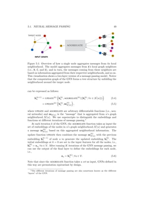
![5.1. NEURAL MESSAGE PASSING 51
5.1.3 The Basic GNN
So far, we have discussed the GNN framework in a relatively abstract fashion as
a series of message-passing iterations using UPDATE and AGGREGATE functions
(Equation 5.4). In order to translate the abstract GNN framework defined
in Equation (5.4) into something we can implement, we must give concrete
instantiations to these UPDATE and AGGREGATE functions. We begin here with
the most basic GNN framework, which is a simplification of the original GNN
models proposed by Merkwirth and Lengauer [2005] and Scarselli et al. [2009].
The basic GNN message passing is defined as
h(k)
u = σ
W
(k)
selfh(k−1)
u + W
(k)
neigh
X
v∈N (u)
h(k−1)
v + b(k)
, (5.7)
where W
(k)
self, W
(k)
neigh ∈ Rd(k)
×d(k−1)
are trainable parameter matrices and σ
denotes an elementwise non-linearity (e.g., a tanh or ReLU). The bias term
b(k)
∈ Rd(k)
is often omitted for notational simplicity, but including the bias
term can be important to achieve strong performance. In this equation—and
throughout the remainder of the book—we use superscripts to differentiate pa-
rameters, embeddings, and dimensionalities in different layers of the GNN.
The message passing in the basic GNN framework is analogous to a standard
multi-layer perceptron (MLP) or Elman-style recurrent neural network, i.e., El-
man RNN [Elman, 1990], as it relies on linear operations followed by a single
elementwise non-linearity. We first sum the messages incoming from the neigh-
bors; then, we combine the neighborhood information with the node’s previous
embedding using a linear combination; and finally, we apply an elementwise
non-linearity.
We can equivalently define the basic GNN through the UPDATE and AGGREGATE
functions:
mN (u) =
X
v∈N (u)
hv, (5.8)
UPDATE(hu, mN (u)) = σ Wselfhu + WneighmN (u)
, (5.9)
where we recall that we use
mN (u) = AGGREGATE
(k)
({h(k)
v , ∀v ∈ N(u)}) (5.10)
as a shorthand to denote the message that has been aggregated from u’s graph
neighborhood. Note also that we omitted the superscript denoting the iteration
in the above equations, which we will often do for notational brevity.2
2In general, the parameters Wself, Wneigh and b can be shared across the GNN message
passing iterations or trained separately for each layer.](https://image.slidesharecdn.com/grlbook-210914153141/85/Grl-book-59-320.jpg)
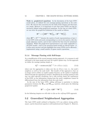
![5.2. GENERALIZED NEIGHBORHOOD AGGREGATION 53
just like a simple MLP or Elman RNN, the basic GNN can be improved upon
and generalized in many ways. Here, we discuss how the AGGREGATE operator
can be generalized and improved upon, with the following section (Section 5.3)
providing an analogous discussion for the UPDATE operation.
5.2.1 Neighborhood Normalization
The most basic neighborhood aggregation operation (Equation 5.8) simply takes
the sum of the neighbor embeddings. One issue with this approach is that it can
be unstable and highly sensitive to node degrees. For instance, suppose node
u has 100× as many neighbors as node u0
(i.e., a much higher degree), then
we would reasonably expect that k
P
v∈N (u) hvk k
P
v0∈N (u0) hv0 k (for any
reasonable vector norm k · k). This drastic difference in magnitude can lead to
numerical instabilities as well as difficulties for optimization.
One solution to this problem is to simply normalize the aggregation operation
based upon the degrees of the nodes involved. The simplest approach is to just
take an average rather than sum:
mN (u) =
P
v∈N (u) hv
|N(u)|
, (5.14)
but researchers have also found success with other normalization factors, such as
the following symmetric normalization employed by Kipf and Welling [2016a]:
mN (u) =
X
v∈N (u)
hv
p
|N(u)||N(v)|
. (5.15)
For example, in a citation graph—the kind of data that Kipf and Welling [2016a]
analyzed—information from very high-degree nodes (i.e., papers that are cited
many times) may not be very useful for inferring community membership in the
graph, since these papers can be cited thousands of times across diverse sub-
fields. Symmetric normalization can also be motivated based on spectral graph
theory. In particular, combining the symmetric-normalized aggregation (Equa-
tion 5.15) along with the basic GNN update function (Equation 5.9) results in
a first-order approximation of a spectral graph convolution, and we expand on
this connection in Chapter 7.
Graph convolutional networks (GCNs)
One of the most popular baseline graph neural network models—the graph
convolutional network (GCN)—employs the symmetric-normalized aggregation
as well as the self-loop update approach. The GCN model thus defines the
message passing function as
h(k)
u = σ
W(k)
X
v∈N (u)∪{u}
hv
p
|N(u)||N(v)|
. (5.16)](https://image.slidesharecdn.com/grlbook-210914153141/85/Grl-book-61-320.jpg)
![54 CHAPTER 5. THE GRAPH NEURAL NETWORK MODEL
This approach was first outlined by Kipf and Welling [2016a] and has proved to
be one of the most popular and effective baseline GNN architectures.
To normalize or not to normalize? Proper normalization can be es-
sential to achieve stable and strong performance when using a GNN. It
is important to note, however, that normalization can also lead to a loss
of information. For example, after normalization, it can be hard (or even
impossible) to use the learned embeddings to distinguish between nodes
of different degrees, and various other structural graph features can be
obscured by normalization. In fact, a basic GNN using the normalized ag-
gregation operator in Equation (5.14) is provably less powerful than the
basic sum aggregator in Equation (5.8) (see Chapter 7). The use of nor-
malization is thus an application-specific question. Usually, normalization
is most helpful in tasks where node feature information is far more useful
than structural information, or where there is a very wide range of node
degrees that can lead to instabilities during optimization.
5.2.2 Set Aggregators
Neighborhood normalization can be a useful tool to improve GNN performance,
but can we do more to improve the AGGREGATE operator? Is there perhaps
something more sophisticated than just summing over the neighbor embeddings?
The neighborhood aggregation operation is fundamentally a set function.
We are given a set of neighbor embeddings {hv, ∀v ∈ N(u)} and must map this
set to a single vector mN (u). The fact that {hv, ∀v ∈ N(u)} is a set is in fact
quite important: there is no natural ordering of a nodes’ neighbors, and any
aggregation function we define must thus be permutation invariant.
Set pooling
One principled approach to define an aggregation function is based on the theory
of permutation invariant neural networks. For example, Zaheer et al. [2017] show
that an aggregation function with the following form is a universal set function
approximator:
mN (u) = MLPθ
X
v∈N(u)
MLPφ(hv)
, (5.17)
where as usual we use MLPθ to denote an arbitrarily deep multi-layer perceptron
parameterized by some trainable parameters θ. In other words, the theoretical
results in Zaheer et al. [2017] show that any permutation-invariant function
that maps a set of embeddings to a single embedding can be approximated to
an arbitrary accuracy by a model following Equation (5.17).
Note that the theory presented in Zaheer et al. [2017] employs a sum of the
embeddings after applying the first MLP (as in Equation 5.17). However, it is
possible to replace the sum with an alternative reduction function, such as an](https://image.slidesharecdn.com/grlbook-210914153141/85/Grl-book-62-320.jpg)
![5.2. GENERALIZED NEIGHBORHOOD AGGREGATION 55
element-wise maximum or minimum, as in Qi et al. [2017], and it is also common
to combine models based on Equation (5.17) with the normalization approaches
discussed in Section 5.2.1, as in the GraphSAGE-pool approach [Hamilton et al.,
2017b].
Set pooling approaches based on Equation (5.17) often lead to small increases
in performance, though they also introduce an increased risk of overfitting,
depending on the depth of the MLPs used. If set pooling is used, it is common to
use MLPs that have only a single hidden layer, since these models are sufficient
to satisfy the theory, but are not so overparameterized so as to risk catastrophic
overfitting.
Janossy pooling
Set pooling approaches to neighborhood aggregation essentially just add extra
layers of MLPs on top of the more basic aggregation architectures discussed
in Section 5.1.3. This idea is simple, but is known to increase the theoretical
capacity of GNNs. However, there is another alternative approach, termed
Janossy pooling, that is also provably more powerful than simply taking a sum
or mean of the neighbor embeddings [Murphy et al., 2018].
Recall that the challenge of neighborhood aggregation is that we must use
a permutation-invariant function, since there is no natural ordering of a node’s
neighbors. In the set pooling approach (Equation 5.17), we achieved this permu-
tation invariance by relying on a sum, mean, or element-wise max to reduce the
set of embeddings to a single vector. We made the model more powerful by com-
bining this reduction with feed-forward neural networks (i.e., MLPs). Janossy
pooling employs a different approach entirely: instead of using a permutation-
invariant reduction (e.g., a sum or mean), we apply a permutation-sensitive
function and average the result over many possible permutations.
Let πi ∈ Π denote a permutation function that maps the set {hv, ∀v ∈ N(u)}
to a specific sequence (hv1
, hv2
, ..., hv|N (u)|
)πi
. In other words, πi takes the
unordered set of neighbor embeddings and places these embeddings in a sequence
based on some arbitrary ordering. The Janossy pooling approach then performs
neighborhood aggregation by
mN (u) = MLPθ
1
|Π|
X
π∈Π
ρφ hv1
, hv2
, ..., hv|N (u)|
πi
!
, (5.18)
where Π denotes a set of permutations and ρφ is a permutation-sensitive func-
tion, e.g., a neural network that operates on sequences. In practice ρφ is usually
defined to be an LSTM [Hochreiter and Schmidhuber, 1997], since LSTMs are
known to be a powerful neural network architecture for sequences.
If the set of permutations Π in Equation (5.18) is equal to all possible per-
mutations, then the aggregator in Equation (5.18) is also a universal function
approximator for sets, like Equation (5.17). However, summing over all pos-
sible permutations is generally intractable. Thus, in practice, Janossy pooling
employs one of two approaches:](https://image.slidesharecdn.com/grlbook-210914153141/85/Grl-book-63-320.jpg)
![56 CHAPTER 5. THE GRAPH NEURAL NETWORK MODEL
1. Sample a random subset of possible permutations during each application
of the aggregator, and only sum over that random subset.
2. Employ a canonical ordering of the nodes in the neighborhood set; e.g.,
order the nodes in descending order according to their degree, with ties
broken randomly.
Murphy et al. [2018] include a detailed discussion and empirical comparison of
these two approaches, as well as other approximation techniques (e.g., truncat-
ing the length of sequence), and their results indicate that Janossy-style pooling
can improve upon set pooling in a number of synthetic evaluation setups.
5.2.3 Neighborhood Attention
In addition to more general forms of set aggregation, a popular strategy for
improving the aggregation layer in GNNs is to apply attention [Bahdanau et al.,
2015]. The basic idea is to assign an attention weight or importance to each
neighbor, which is used to weigh this neighbor’s influence during the aggregation
step. The first GNN model to apply this style of attention was Veličković et al.
[2018]’s Graph Attention Network (GAT), which uses attention weights to define
a weighted sum of the neighbors:
mN (u) =
X
v∈N (u)
αu,vhv, (5.19)
where αu,v denotes the attention on neighbor v ∈ N(u) when we are aggregating
information at node u. In the original GAT paper, the attention weights are
defined as
αu,v =
exp a
[Whu ⊕ Whv]
P
v0∈N (u) exp (a[Whu ⊕ Whv0 ])
, (5.20)
where a is a trainable attention vector, W is a trainable matrix, and ⊕ denotes
the concatenation operation.
The GAT-style attention computation is known to work well with graph
data. However, in principle any standard attention model from the deep learning
literature at large can be used [Bahdanau et al., 2015]. Popular variants of
attention include the bilinear attention model
αu,v =
exp h
u Whv
P
v0∈N (u) exp (h
u Whv0 )
, (5.21)
as well as variations of attention layers using MLPs, e.g.,
αu,v =
exp (MLP(hu, hv))
P
v0∈N (u) exp (MLP(hu, hv0 ))
, (5.22)
where the MLP is restricted to a scalar output.
In addition, while it is less common in the GNN literature, it is also possi-
ble to add multiple attention “heads”, in the style of the popular transformer](https://image.slidesharecdn.com/grlbook-210914153141/85/Grl-book-64-320.jpg)
![5.2. GENERALIZED NEIGHBORHOOD AGGREGATION 57
architecture [Vaswani et al., 2017]. In this approach, one computes K distinct
attention weights αu,v,k, using independently parameterized attention layers.
The messages aggregated using the different attention weights are then trans-
formed and combined in the aggregation step, usually with a linear projection
followed by a concatenation operation, e.g.,
mN (u) = [a1 ⊕ a2 ⊕ ... ⊕ aK] (5.23)
ak = Wk
X
v∈N (u)
αu,v,khv (5.24)
where the attention weights αu,v,k for each of the K attention heads can be
computed using any of the above attention mechanisms.
Graph attention and transformers GNN models with multi-headed
attention (Equation 5.23) are closely related to the transformer architecture
[Vaswani et al., 2017]. Transformers are a popular architecture for both
natural language processing (NLP) and computer vision, and—in the case
of NLP—they have been an important driver behind large state-of-the-art
NLP systems, such as BERT [Devlin et al., 2018] and XLNet [Yang et al.,
2019]. The basic idea behind transformers is to define neural network layers
entirely based on the attention operation. At each layer in a transformer,
a new hidden representation is generated for every position in the input
data (e.g., every word in a sentence) by using multiple attention heads to
compute attention weights between all pairs of positions in the input, which
are then aggregated with weighted sums based on these attention weights
(in a manner analogous to Equation 5.23). In fact, the basic transformer
layer is exactly equivalent to a GNN layer using multi-headed attention
(i.e., Equation 5.23) if we assume that the GNN receives a fully-connected
graph as input.
This connection between GNNs and transformers has been exploited in
numerous works. For example, one implementation strategy for designing
GNNs is to simply start with a transformer model and then apply a bi-
nary adjacency mask on the attention layer to ensure that information is
only aggregated between nodes that are actually connected in the graph.
This style of GNN implementation can benefit from the numerous well-
engineered libraries for transformer architectures that exist. However, a
downside of this approach, is that transformers must compute the pair-
wise attention between all positions/nodes in the input, which leads to a
quadratic O(|V|2
) time complexity to aggregate messages for all nodes in
the graph, compared to a O(|V||E|) time complexity for a more standard
GNN implementation.
Adding attention is a useful strategy for increasing the representational ca-
pacity of a GNN model, especially in cases where you have prior knowledge
to indicate that some neighbors might be more informative than others. For
example, consider the case of classifying papers into topical categories based](https://image.slidesharecdn.com/grlbook-210914153141/85/Grl-book-65-320.jpg)
![58 CHAPTER 5. THE GRAPH NEURAL NETWORK MODEL
on citation networks. Often there are papers that span topical boundaries, or
that are highly cited across various different fields. Ideally, an attention-based
GNN would learn to ignore these papers in the neural message passing, as such
promiscuous neighbors would likely be uninformative when trying to identify
the topical category of a particular node. In Chapter 7, we will discuss how
attention can influence the inductive bias of GNNs from a signal processing
perspective.
5.3 Generalized Update Methods
The AGGREGATE operator in GNN models has generally received the most atten-
tion from researchers—in terms of proposing novel architectures and variations.
This was especially the case after the introduction of the GraphSAGE framework,
which introduced the idea of generalized neighbourhood aggregation [Hamilton
et al., 2017b]. However, GNN message passing involves two key steps: aggre-
gation and updating, and in many ways the UPDATE operator plays an equally
important role in defining the power and inductive bias of the GNN model.
So far, we have seen the basic GNN approach—where the update operation
involves a linear combination of the node’s current embedding with the message
from its neighbors—as well as the self-loop approach, which simply involves
adding a self-loop to the graph before performing neighborhood aggregation. In
this section, we turn our attention to more diverse generalizations of the UPDATE
operator.
Over-smoothing and neighbourhood influence One common issue
with GNNs—which generalized update methods can help to address—is
known as over-smoothing. The essential idea of over-smoothing is that after
several iterations of GNN message passing, the representations for all the
nodes in the graph can become very similar to one another. This tendency is
especially common in basic GNN models and models that employ the self-
loop update approach. Over-smoothing is problematic because it makes
it impossible to build deeper GNN models—which leverage longer-term
dependencies in the graph—since these deep GNN models tend to just
generate over-smoothed embeddings.
This issue of over-smoothing in GNNs can be formalized by defining the
influence of each node’s input feature h
(0)
u = xu on the final layer embedding
of all the other nodes in the graph, i.e, h
(K)
v , ∀v ∈ V. In particular, for any
pair of nodes u and v we can quantify the influence of node u on node v
in the GNN by examining the magnitude of the corresponding Jacobian
matrix [Xu et al., 2018]:
IK(u, v) = 1 ∂h
(K)
v
∂h
(0)
u
!
1, (5.25)
where 1 is a vector of all ones. The IK(u, v) value uses the sum of the](https://image.slidesharecdn.com/grlbook-210914153141/85/Grl-book-66-320.jpg)
![5.3. GENERALIZED UPDATE METHODS 59
entries in the Jacobian matrix
∂h(K)
v
∂h
(0)
u
as a measure of how much the initial
embedding of node u influences the final embedding of node v in the GNN.
Given this definition of influence, Xu et al. [2018] prove the following:
Theorem 3. For any GNN model using a self-loop update approach and
an aggregation function of the form
AGGREGATE({hv, ∀v ∈ N(u) ∪ {u}}) =
1
fn(|N(u) ∪ {u}|)
X
v∈N (u)∪{u}
hv,
(5.26)
where f : R+
→ R+
is an arbitrary differentiable normalization function,
we have that
IK(u, v) ∝ pG,K(u|v), (5.27)
where pG,K(u|v) denotes the probability of visiting node v on a length-K
random walk starting from node u.
This theorem is a direct consequence of Theorem 1 in Xu et al. [2018].
It states that when we are using a K-layer GCN-style model, the influ-
ence of node u and node v is proportional the probability of reaching node
v on a K-step random walk starting from node u. An important conse-
quence of this, however, is that as K → ∞ the influence of every node
approaches the stationary distribution of random walks over the graph,
meaning that local neighborhood information is lost. Moreover, in many
real-world graphs—which contain high-degree nodes and resemble so-called
“expander” graphs—it only takes k = O(log(|V|) steps for the random
walk starting from any node to converge to an almost-uniform distribution
[Hoory et al., 2006].
Theorem 3 applies directly to models using a self-loop update approach,
but the result can also be extended in asympotic sense for the basic GNN
update (i.e., Equation 5.9) as long as kW
(k)
selfk kW
(k)
neighk at each layer
k. Thus, when using simple GNN models—and especially those with the
self-loop update approach—building deeper models can actually hurt per-
formance. As more layers are added we lose information about local neigh-
borhood structures and our learned embeddings become over-smoothed,
approaching an almost-uniform distribution.
5.3.1 Concatenation and Skip-Connections
As discussed above, over-smoothing is a core issue in GNNs. Over-smoothing
occurs when node-specific information becomes “washed out” or “lost” after
several iterations of GNN message passing. Intuitively, we can expect over-
smoothing in cases where the information being aggregated from the node
neighbors during message passing begins to dominate the updated node rep-
resentations. In these cases, the updated node representations (i.e., the h
(k+1)
u](https://image.slidesharecdn.com/grlbook-210914153141/85/Grl-book-67-320.jpg)
![60 CHAPTER 5. THE GRAPH NEURAL NETWORK MODEL
vectors) will depend too strongly on the incoming message aggregated from the
neighbors (i.e., the mN (u) vectors) at the expense of the node representations
from the previous layers (i.e., the h
(k)
u vectors). A natural way to alleviate this
issue is to use vector concatenations or skip connections, which try to directly
preserve information from previous rounds of message passing during the update
step.
These concatenation and skip-connection methods can be used in conjunc-
tion with most other GNN update approaches. Thus, for the sake of generality,
we will use UPDATEbase to denote the base update function that we are building
upon (e.g., we can assume that UPDATEbase is given by Equation 5.9), and we
will define various skip-connection updates on top of this base function.
One of the simplest skip connection updates employs a concatenation to
preserve more node-level information during message passing:
UPDATEconcat(hu, mN (u)) = [UPDATEbase(hu, mN (u)) ⊕ hu], (5.28)
where we simply concatenate the output of the base update function with
the node’s previous-layer representation. Again, the key intuition here is that
we encourage the model to disentangle information during message passing—
separating the information coming from the neighbors (i.e., mN (u)) from the
current representation of each node (i.e., hu).
The concatenation-based skip connection was proposed in the GraphSAGE
framework, which was one of the first works to highlight the possible benefits
of these kinds of modifications to the update function [Hamilton et al., 2017a].
However, in addition to concatenation, we can also employ other forms of skip-
connections, such as the linear interpolation method proposed by Pham et al.
[2017]:
UPDATEinterpolate(hu, mN (u)) = α1 ◦ UPDATEbase(hu, mN (u)) + α2](https://image.slidesharecdn.com/grlbook-210914153141/85/Grl-book-68-320.jpg)
![hu, (5.29)
where α1, α2 ∈ [0, 1]d
are gating vectors with α2 = 1 − α1 and ◦ denotes el-
ementwise multiplication. In this approach, the final updated representation
is a linear interpolation between the previous representation and the represen-
tation that was updated based on the neighborhood information. The gating
parameters α1 can be learned jointly with the model in a variety of ways. For
example, Pham et al. [2017] generate α1 as the output of a separate single-layer
GNN, which takes the current hidden-layer representations as features. How-
ever, other simpler approaches could also be employed, such as simply directly
learning α1 parameters for each message passing layer or using an MLP on the
current node representations to generate these gating parameters.
In general, these concatenation and residual connections are simple strate-
gies that can help to alleviate the over-smoothing issue in GNNs, while also
improving the numerical stability of optimization. Indeed, similar to the util-
ity of residual connections in convolutional neural networks (CNNs) [He et al.,
2016], applying these approaches to GNNs can facilitate the training of much
deeper models. In practice these techniques tend to be most useful for node](https://image.slidesharecdn.com/grlbook-210914153141/85/Grl-book-69-320.jpg)
![5.3. GENERALIZED UPDATE METHODS 61
classification tasks with moderately deep GNNs (e.g., 2-5 layers), and they ex-
cel on tasks that exhibit homophily, i.e., where the prediction for each node is
strongly related to the features of its local neighborhood.
5.3.2 Gated Updates
In the previous section we discussed skip-connection and residual connection
approaches that bear strong analogy to techniques used in computer vision to
build deeper CNN architectures. In a parallel line of work, researchers have also
drawn inspiration from the gating methods used to improve the stability and
learning ability of recurrent neural networks (RNNs). In particular, one way
to view the GNN message passing algorithm is that the aggregation function
is receiving an observation from the neighbors, which is then used to update
the hidden state of each node. In this view, we can directly apply methods
used to update the hidden state of RNN architectures based on observations.
For instance, one of the earliest GNN architectures [Li et al., 2015] defines the
update function as
h(k)
u = GRU(h(k−1)
u , m
(k)
N (u)), (5.30)
where GRU denotes the update equation of the gated recurrent unit (GRU)
cell [Cho et al., 2014]. Other approaches have employed updates based on the
LSTM architecture [Selsam et al., 2019].
In general, any update function defined for RNNs can be employed in the
context of GNNs. We simply replace the hidden state argument of the RNN
update function (usually denoted h(t)
) with the node’s hidden state, and we re-
place the observation vector (usually denoted x(t)
) with the message aggregated
from the local neighborhood. Importantly, the parameters of this RNN-style up-
date are always shared across nodes (i.e., we use the same LSTM or GRU cell
to update each node). In practice, researchers usually share the parameters of
the update function across the message-passing layers of the GNN as well.
These gated updates are very effective at facilitating deep GNN architectures
(e.g., more than 10 layers) and preventing over-smoothing. Generally, they are
most useful for GNN applications where the prediction task requires complex
reasoning over the global structure of the graph, such as applications for program
analysis [Li et al., 2015] or combinatorial optimization [Selsam et al., 2019].
5.3.3 Jumping Knowledge Connections
In the preceding sections, we have been implicitly assuming that we are using
the output of the final layer of the GNN. In other words, we have been assuming
that the node representations zu that we use in a downstream task are equal to
final layer node embeddings in the GNN:
zu = h(K)
u , ∀u ∈ V. (5.31)
This assumption is made by many GNN approaches, and the limitations of this
strategy motivated much of the need for residual and gated updates to limit
over-smoothing.](https://image.slidesharecdn.com/grlbook-210914153141/85/Grl-book-70-320.jpg)
![62 CHAPTER 5. THE GRAPH NEURAL NETWORK MODEL
However, a complimentary strategy to improve the quality of the final node
representations is to simply leverage the representations at each layer of message
passing, rather than only using the final layer output. In this approach we define
the final node representations zu as
zu = fJK(h(0)
u ⊕ h(1)
u ⊕ ... ⊕ h(K)
u ), (5.32)
where fJK is an arbitrary differentiable function. This strategy is known as
adding jumping knowledge (JK) connections and was first proposed and ana-
lyzed by Xu et al. [2018]. In many applications the function fJK can simply
be defined as the identity function, meaning that we just concatenate the node
embeddings from each layer, but Xu et al. [2018] also explore other options
such as max-pooling approaches and LSTM attention layers. This approach
often leads to consistent improvements across a wide-variety of tasks and is a
generally useful strategy to employ.
5.4 Edge Features and Multi-relational GNNs
So far our discussion of GNNs and neural message passing has implicitly assumed
that we have simple graphs. However, there are many applications where the
graphs in question are multi-relational or otherwise heterogenous (e.g., knowl-
edge graphs). In this section, we review some of the most popular strategies
that have been developed to accommodate such data.
5.4.1 Relational Graph Neural Networks
The first approach proposed to address this problem is commonly known as
the Relational Graph Convolutional Network (RGCN) approach [Schlichtkrull
et al., 2017]. In this approach we augment the aggregation function to accom-
modate multiple relation types by specifying a separate transformation matrix
per relation type:
mN (u) =
X
τ∈R
X
v∈Nτ (u)
Wτ hv
fn(N(u), N(v))
, (5.33)
where fn is a normalization function that can depend on both the neighborhood
of the node u as well as the neighbor v being aggregated over. Schlichtkrull et al.
[2017] discuss several normalization strategies to define fn that are analagous
to those discussed in Section 5.2.1. Overall, the multi-relational aggregation in
RGCN is thus analagous to the basic a GNN approach with normalization, but
we separately aggregate information across different edge types.
Parameter sharing
One drawback of the naive RGCN approach is the drastic increase in the number
of parameters, as now we have one trainable matrix per relation type. In cer-
tain applications—such as applications on knowledge graphs with many distinct](https://image.slidesharecdn.com/grlbook-210914153141/85/Grl-book-71-320.jpg)
![5.4. EDGE FEATURES AND MULTI-RELATIONAL GNNS 63
relations—this increase in parameters can lead to overfitting and slow learning.
Schlichtkrull et al. [2017] propose a scheme to combat this issue by parameter
sharing with basis matrices, where
Wτ =
b
X
i=1
αi,τ Bi. (5.34)
In this basis matrix approach, all the relation matrices are defined as linear
combinations of b basis matrices B1, ..., Bb, and the only relation-specific pa-
rameters are the b combination weights α1,τ , ..., αb,τ for each relation τ. In this
basis sharing approach, we can thus rewrite the full aggregation function as
mN (u) =
X
τ∈R
X
v∈Nτ (u)
ατ ×1 B ×2 hv
fn(N(u), N(v))
, (5.35)
where B = (B1, ..., Bb) is a tensor formed by stacking the basis matrices, ατ =
(α1,τ , ..., αb,τ ) is a vector containing the basis combination weights for relation
τ, and ×i denotes a tensor product along mode i. Thus, an alternative view of
the parameter sharing RGCN approach is that we are learning an embedding
for each relation, as well a tensor that is shared across all relations.
Extensions and variations
The RGCN architecture can be extended in many ways, and in general, we
refer to approaches that define separate aggregation matrices per relation as
relational graph neural networks. For example, a variation of this approach
without parameter sharing is deployed by Zitnik et al. [2018] to model a multi-
relational dataset relating drugs, diseases and proteins, and a similar strategy
is leveraged by Marcheggiani and Titov [2017] to analyze linguistic dependency
graphs. Other works have found success combining the RGCN-style aggregation
with attention [Teru et al., 2020].
5.4.2 Attention and Feature Concatenation
The relational GNN approach, where we define a separate aggregation param-
eter per relation, is applicable for multi-relational graphs and cases where we
have discrete edge features. To accommodate cases where we have more general
forms of edge features, we can leverage these features in attention or by concate-
nating this information with the neighbor embeddings during message passing.
For example, given any base aggregation approach AGGREGATEbase one simple
strategy to leverage edge features is to define a new aggregation function as
mN (u) = AGGREGATEbase({hv ⊕ e(u,τ,v), ∀v ∈ N(u)}), (5.36)
where e(u,τ,v) denotes an arbitrary vector-valued feature for the edge (u, τ, v).
This approach is simple and general, and has seen recent success with attention-
based approaches as the base aggregation function [Sinha et al., 2019].](https://image.slidesharecdn.com/grlbook-210914153141/85/Grl-book-72-320.jpg)
![64 CHAPTER 5. THE GRAPH NEURAL NETWORK MODEL
5.5 Graph Pooling
The neural message passing approach produces a set of node embeddings, but
what if we want to make predictions at the graph level? In other words, we
have been assuming that the goal is to learn node representations zu, ∀u ∈ V,
but what if we to learn an embedding zG for the entire graph G? This task is
often referred to as graph pooling, since our goal is to pool together the node
embeddings in order to learn an embedding of the entire graph.
Set pooling approaches
Similar to the AGGREGATE operator, the task of graph pooling can be viewed
as a problem of learning over sets. We want to design a pooling function fp,
which maps a set of node embeddings {z1, ..., z|V |} to an embedding zG that
represents the full graph. Indeed, any of the approaches discussed in Section
5.2.2 for learning over sets of neighbor embeddings can also be employed for
pooling at the graph level.
In practice, there are two approaches that are most commonly applied for
learning graph-level embeddings via set pooling. The first approach is simply
to take a sum (or mean) of the node embeddings:
zG =
P
v∈V zu
fn(|V|)
, (5.37)
where fn is some normalizing function (e.g., the identity function). While quite
simple, pooling based on the sum or mean of the node embeddings is often
sufficient for applications involving small graphs.
The second popular set-based approach uses a combination of LSTMs and
attention to pool the node embeddings, in a manner inspired by the work of
Vinyals et al. [2015]. In this pooling approach, we iterate a series of attention-
based aggregations defined by the following set of equations, which are iterated
for t = 1, ..., T steps:
qt = LSTM(ot−1, qt−1), (5.38)
ev,t = fa(zv, qt), ∀v ∈ V, (5.39)
av,t =
exp(ev,i)
P
u∈V exp(eu,t)
, ∀v ∈ V, (5.40)
ot =
X
v∈V
av,tzv. (5.41)
In the above equations, the qt vector represents a query vector for the attention
at each iteration t. In Equation (5.39), the query vector is used to compute an
attention score over each node using an attention function fa : Rd
× Rd
→ R
(e.g., a dot product), and this attention score is then normalized in Equation
(5.40). Finally, in Equation (5.41) a weighted sum of the node embeddings is
computed based on the attention weights, and this weighted sum is used to](https://image.slidesharecdn.com/grlbook-210914153141/85/Grl-book-73-320.jpg)
![5.5. GRAPH POOLING 65
update the query vector using an LSTM update (Equation 5.38). Generally
the q0 and o0 vectors are initialized with all-zero values, and after iterating
Equations (5.38)-(5.41) for T iterations, an embedding for the full graph is
computed as
zG = o1 ⊕ o2 ⊕ ... ⊕ oT . (5.42)
This approach represents a sophisticated architecture for attention-based pool-
ing over a set, and it has become a popular pooling method in many graph-level
classification tasks.
Graph coarsening approaches
One limitation of the set pooling approaches is that they do not exploit the struc-
ture of the graph. While it is reasonable to consider the task of graph pooling
as simply a set learning problem, there can also be benefits from exploiting
the graph topology at the pooling stage. One popular strategy to accomplish
this is to perform graph clustering or coarsening as a means to pool the node
representations.
In these style of approaches, we assume that we have some clustering function
fc → G × R|V |×d
→ R+|V |×c
, (5.43)
which maps all the nodes in the graph to an assignment over c clusters. In
particular, we presume that this function outputs an assignment matrix S =
fc(G, Z), where S[u, i] ∈ R+
denotes the strength of the association between
node u and cluster i. One simple example of an fc function would be spectral
clustering approach described in Chapter 1, where the cluster assignment is
based on the spectral decomposition of the graph adjacency matrix. In a more
complex definition of fc, one can actually employ another GNN to predict cluster
assignments [Ying et al., 2018b].
Regardless of the approach used to generate the cluster assignment matrix
S, the key idea of graph coarsening approaches is that we then use this matrix
to coarsen the graph. In particular, we use the assignment matrix S to compute
a new coarsened adjacency matrix
Anew
= S
AS ∈ R+c×c
(5.44)
and a new set of node features
Xnew
= S
X ∈ Rc×d
. (5.45)
Thus, this new adjacency matrix now represents the strength of association
(i.e., the edges) between the clusters in the graph, and the new feature matrix
represents the aggregated embeddings for all the nodes assigned to each cluster.
We can then run a GNN on this coarsened graph and repeat the entire coarsening
process for a number of iterations, where the size of the graph is decreased at
each step. The final representation of the graph is then computed by a set
pooling over the embeddings of the nodes in a sufficiently coarsened graph.](https://image.slidesharecdn.com/grlbook-210914153141/85/Grl-book-74-320.jpg)
![66 CHAPTER 5. THE GRAPH NEURAL NETWORK MODEL
This coarsening based approach is inspired by the pooling approaches used
in convolutional neural networks (CNNs), and it relies on the intuition that we
can build hierarchical GNNs that operate on different granularities of the input
graph. In practice, these coarsening approaches can lead to strong performance,
but they can also be unstable and difficult to train. For example, in order
to have the entire learning process be end-to-end differentiable the clustering
functions fc must be differentiable, which rules out most off-the-shelf clustering
algorithms such as spectral clustering. There are also approaches that coarsen
the graph by selecting a set of nodes to remove rather than pooling all nodes
into clusters, which can lead to benefits in terms of computational complexity
and speed [Cangea et al., 2018, Gao and Ji, 2019].
5.6 Generalized Message Passing
The presentation in this chapter so far has focused on the most popular style
of GNN message passing, which operates largely at the node level. However,
the GNN message passing approach can also be generalized to leverage edge
and graph-level information at each stage of message passing. For example, in
the more general approach proposed by Battaglia et al. [2018], we define each
iteration of message passing according to the following equations:
h
(k)
(u,v) = UPDATEedge(h
(k−1)
(u,v) , h(k−1)
u , h(k−1)
v , h
(k−1)
G ) (5.46)
mN (u) = AGGREGATEnode({h
(k)
(u,v)∀v ∈ N(u)}) (5.47)
h(k)
u = UPDATEnode(h(k−1)
u , mN (u), h
(k−1)
G ) (5.48)
h
(k)
G = UPDATEgraph(h
(k−1)
G , {h(k)
u , ∀u ∈ V}, {h
(k)
(u,v)∀(u, v) ∈ E}). (5.49)
The important innovation in this generalized message passing framework is that,
during message passing, we generate hidden embeddings h
(k)
(u,v) for each edge in
the graph, as well as an embedding h
(k)
G corresponding to the entire graph. This
allows the message passing model to easily integrate edge and graph-level fea-
tures, and recent work has also shown this generalized message passing approach
to have benefits compared to a standard GNN in terms of logical expressiveness
[Barceló et al., 2020]. Generating embeddings for edges and the entire graph
during message passing also makes it trivial to define loss functions based on
graph or edge-level classification tasks.
In terms of the message-passing operations in this generalized message-
passing framework, we first update the edge embeddings based on the embed-
dings of their incident nodes (Equation 5.46). Next, we update the node embed-
dings by aggregating the edge embeddings for all their incident edges (Equations
5.47 and 5.48). The graph embedding is used in the update equation for both
node and edge representations, and the graph-level embedding itself is updated
by aggregating over all the node and edge embeddings at the end of each iter-
ation (Equation 5.49). All of the individual update and aggregation operations](https://image.slidesharecdn.com/grlbook-210914153141/85/Grl-book-75-320.jpg)
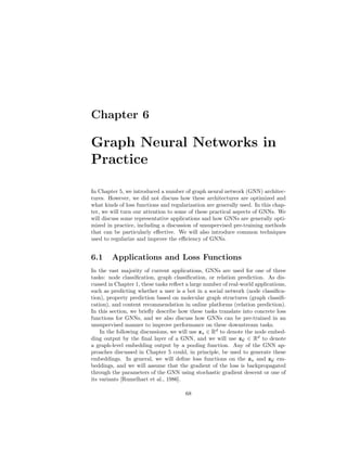
![Chapter 6
Graph Neural Networks in
Practice
In Chapter 5, we introduced a number of graph neural network (GNN) architec-
tures. However, we did not discuss how these architectures are optimized and
what kinds of loss functions and regularization are generally used. In this chap-
ter, we will turn our attention to some of these practical aspects of GNNs. We
will discuss some representative applications and how GNNs are generally opti-
mized in practice, including a discussion of unsupervised pre-training methods
that can be particularly effective. We will also introduce common techniques
used to regularize and improve the efficiency of GNNs.
6.1 Applications and Loss Functions
In the vast majority of current applications, GNNs are used for one of three
tasks: node classification, graph classification, or relation prediction. As dis-
cussed in Chapter 1, these tasks reflect a large number of real-world applications,
such as predicting whether a user is a bot in a social network (node classifica-
tion), property prediction based on molecular graph structures (graph classifi-
cation), and content recommendation in online platforms (relation prediction).
In this section, we briefly describe how these tasks translate into concrete loss
functions for GNNs, and we also discuss how GNNs can be pre-trained in an
unsupervised manner to improve performance on these downstream tasks.
In the following discussions, we will use zu ∈ Rd
to denote the node embed-
ding output by the final layer of a GNN, and we will use zG ∈ Rd
to denote
a graph-level embedding output by a pooling function. Any of the GNN ap-
proaches discussed in Chapter 5 could, in principle, be used to generate these
embeddings. In general, we will define loss functions on the zu and zG em-
beddings, and we will assume that the gradient of the loss is backpropagated
through the parameters of the GNN using stochastic gradient descent or one of
its variants [Rumelhart et al., 1986].
68](https://image.slidesharecdn.com/grlbook-210914153141/85/Grl-book-77-320.jpg)
![6.1. APPLICATIONS AND LOSS FUNCTIONS 69
6.1.1 GNNs for Node Classification
Node classification is one of the most popular benchmark tasks for GNNs. For
instance, during the years 2017 to 2019—when GNN methods were beginning
to gain prominence across machine learning—research on GNNs was dominated
by the Cora, Citeseer, and Pubmed citation network benchmarks, which were
popularized by Kipf and Welling [2016a]. These baselines involved classifying
the category or topic of scientific papers based on their position within a citation
network, with language-based node features (e.g., word vectors) and only a very
small number of positive examples given per each class (usually less than 10%
of the nodes).
The standard way to apply GNNs to such a node classification task is to train
GNNs in a fully-supervised manner, where we define the loss using a softmax
classification function and negative log-likelihood loss:
L =
X
u∈Vtrain
− log(softmax(zu, yu)). (6.1)
Here, we assume that yu ∈ Zc
is a one-hot vector indicating the class of training
node u ∈ Vtrain; for example, in the citation network setting, yu would indicate
the topic of paper u. We use softmax(zu, yu) to denote the predicted probability
that the node belongs to the class yu, computed via the softmax function:
softmax(zu, yu) =
c
X
i=1
yu[i]
ez
u wi
Pc
j=1 ez
u wj
, (6.2)
where wi ∈ Rd
, i = 1, ..., c are trainable parameters. There are other variations
of supervised node losses, but training GNNs in a supervised manner based on
the loss in Equation (6.1) is one of the most common optimization strategies for
GNNs.
Supervised, semi-supervised, transductive, and inductive Note
that—as discussed in Chapter 1—the node classification setting is often
referred to both as supervised and semi-supervised. One important factor
when applying these terms is whether and how different nodes are used
during training the GNN. Generally, we can distinguish between three types
of nodes:
1. There is the set of training nodes, Vtrain. These nodes are included
in the GNN message passing operations, and they are also used to
compute the loss, e.g., via Equation (6.1).
2. In addition to the training nodes, we can also have transductive test
nodes, Vtrans. These nodes are unlabeled and not used in the loss
computation, but these nodes—and their incident edges—are still
involved in the GNN message passing operations. In other words,
the GNN will generate hidden representations h
(k)
u for the nodes in
u ∈ Vtrans during the GNN message passing operations. However, the](https://image.slidesharecdn.com/grlbook-210914153141/85/Grl-book-78-320.jpg)
![70 CHAPTER 6. GRAPH NEURAL NETWORKS IN PRACTICE
final layer embeddings zu for these nodes will not be used in the loss
function computation.
3. Finally, we will also have inductive test nodes, Vind. These nodes are
not used in either the loss computation or the GNN message passing
operations during training, meaning that these nodes—and all of their
edges—are completely unobserved while the GNN is trained.
The term semi-supervised is applicable in cases where the GNN is tested
on transductive test nodes, since in this case the GNN observes the test
nodes (but not their labels) during training. The term inductive node
classification is used to distinguish the setting where the test nodes—and
all their incident edges—are completely unobserved during training. An
example of inductive node classification would be training a GNN on one
subgraph of a citation network and then testing it on a completely disjoint
subgraph.
6.1.2 GNNs for Graph Classification
Similar to node classification, applications on graph-level classification are pop-
ular as benchmark tasks. Historically, kernel methods were popular for graph
classification, and—as a result—some of the most popular early benchmarks
for graph classification were adapted from the kernel literature, such as tasks
involving the classification of enzyme properties based on graph-based repre-
sentations [Morris et al., 2019]. In these tasks, a softmax classification loss—
analogous to Equation (6.1)—is often used, with the key difference that the
loss is computed with graph-level embeddings zGi
over a set of labeled training
graphs T = {G1, ..., Gn}. In recent years, GNNs have also witnessed success
in regression tasks involving graph data—especially tasks involving the predic-
tion of molecular properties (e.g., solubility) from graph-based representations
of molecules. In these instances, it is standard to employ a squared-error loss
of the following form:
L =
X
Gi∈T
kMLP(zGi
) − yGi
k2
2, (6.3)
where MLP is a densely connected neural network with a univariate output and
yGi ∈ R is the target value for training graph Gi.
6.1.3 GNNs for Relation Prediction
While classification tasks are by far the most popular application of GNNs,
GNNs are also used in in relation prediction tasks, such as recommender systems
[Ying et al., 2018a] and knowledge graph completion [Schlichtkrull et al., 2017].
In these applications, the standard practice is to employ the pairwise node
embedding loss functions introduced in Chapters 3 and 4. In principle, GNNs](https://image.slidesharecdn.com/grlbook-210914153141/85/Grl-book-79-320.jpg)
![6.1. APPLICATIONS AND LOSS FUNCTIONS 71
can be combined with any of the pairwise loss functions discussed in those
chapters, with the output of the GNNs replacing the shallow embeddings.
6.1.4 Pre-training GNNs
Pre-training techniques have become standard practice in deep learning [Good-
fellow et al., 2016]. In the case of GNNs, one might imagine that pre-training
a GNN using one of the neighborhood reconstruction losses from Chapter 3
could be a useful strategy to improve performance on a downstream classifica-
tion task. For example, one could pre-train a GNN to reconstruct missing edges
in the graph before fine-tuning on a node classification loss.
Interestingly, however, this approach has achieved little success in the con-
text of GNNs. In fact, Veličković et al. [2019] even find that a randomly ini-
tialized GNN is equally strong compared to one pre-trained on a neighborhood
reconstruction loss. One hypothesis to explain this finding is the fact that the
GNN message passing already effectively encodes neighborhood information.
Neighboring nodes in the graph will tend to have similar embeddings in a GNN
due to the structure of message passing, so enforcing a neighborhood recon-
struction loss can simply be redundant.
Despite this negative result regarding pre-training with neighborhood re-
construction losses, there have been positive results using other pre-training
strategies. For example, Veličković et al. [2019] propose Deep Graph Infomax
(DGI), which involves maximizing the mutual information between node em-
beddings zu and graph embeddings zG. Formally, this approach optimizes the
following loss:
L = −
X
u∈Vtrain
EG log(D(zu, zG)) + γEG̃ log(1 − D(z̃u, zG)). (6.4)
Here, zu denotes the embedding of node u generated from the GNN based on
graph G, while z̃u denotes an embedding of node u generated based on a cor-
rupted version of graph G, denoted G̃. We use D to denote a discriminator
function, which is a neural network trained to predict whether the node em-
bedding came from the real graph G or the corrupted version G̃. Usually, the
graph is corrupted by modifying either the node features, adjacency matrix, or
both in some stochastic manner (e.g., shuffling entries of the feature matrix).
The intuition behind this loss is that the GNN model must learn to generate
node embeddings that can distinguish between the real graph and its corrupted
counterpart. It can be shown that this optimization is closely connected to
maximizing the mutual information between the node embeddings zu and the
graph-level embedding zG.
The loss function used in DGI (Equation 6.4) is just one example of a broader
class of unsupervised objectives that have witnessed success in the context of
GNNs [Hu et al., 2019, Sun et al., 2020]. These unsupervised training strategies
generally involve training GNNs to maximize the mutual information between
different levels of representations or to distinguish between real and corrupted](https://image.slidesharecdn.com/grlbook-210914153141/85/Grl-book-80-320.jpg)
![72 CHAPTER 6. GRAPH NEURAL NETWORKS IN PRACTICE
pairs of embeddings. Conceptually, these pre-training approaches—which are
also sometimes used as auxiliary losses during supervised training—bear sim-
ilarities to the “content masking” pre-training approaches that have ushered
in a new state of the art in natural language processing [Devlin et al., 2018].
Nonetheless, the extension and improvement of GNN pre-training approaches
is an open and active area of research.
6.2 Efficiency Concerns and Node Sampling
In Chapter 5, we mainly discussed GNNs from the perspective of node-level
message passing equations. However, directly implementing a GNN based on
these equations can be computationally inefficient. For example, if multiple
nodes share neighbors, we might end up doing redundant computation if we
implement the message passing operations independently for all nodes in the
graph. In this section, we discuss some strategies that can be used implement
GNNs in an efficient manner.
6.2.1 Graph-level Implementations
In terms of minimizing the number of mathematical operations needed to run
message passing, the most effective strategy is to use graph-level implemen-
tations of the GNN equations. We discussed these graph-level equations in
Section 5.1.3 of the previous chapter, and the key idea is to implement the mes-
sage passing operations based on sparse matrix multiplications. For example,
the graph-level equation for a basic GNN is given by
H(k)
= σ
AH(k−1)
W
(k)
neigh + H(k−1)
W
(k)
self
, (6.5)
where H(t)
is a matrix containing the layer-k embeddings of all the nodes in
the graph. The benefit of using these equations is that there are no redundant
computations—i.e., we compute the embedding h
(k)
u for each node u exactly
once when running the model. However, the limitation of this approach is that
it requires operating on the entire graph and all node features simultaneously,
which may not be feasible due to memory limitations. In addition, using the
graph-level equations essentially limits one to full-batch (as opposed to mini-
batched) gradient descent.
6.2.2 Subsampling and Mini-Batching
In order to limit the memory footprint of a GNN and facilitate mini-batch
training, one can work with a subset of nodes during message passing. Math-
ematically, we can think of this as running the node-level GNN equations for
a subset of the nodes in the graph in each batch. Redundant computations
can be avoided through careful engineering to ensure that we only compute the](https://image.slidesharecdn.com/grlbook-210914153141/85/Grl-book-81-320.jpg)
![6.3. PARAMETER SHARING AND REGULARIZATION 73
embedding h
(k)
u for each node u in the batch at most once when running the
model.
The challenge, however, is that we cannot simply run message passing on
a subset of the nodes in a graph without losing information. Every time we
remove a node, we also delete its edges (i.e., we modify the adjacency matrix).
There is no guarantee that selecting a random subset of nodes will even lead to
a connected graph, and selecting a random subset of nodes for each mini-batch
can have a severely detrimental impact on model performance.
Hamilton et al. [2017b] propose one strategy to overcome this issue by sub-
sampling node neighborhoods. The basic idea is to first select a set of target
nodes for a batch and then to recursively sample the neighbors of these nodes
in order to ensure that the connectivity of the graph is maintained. In order to
avoid the possibility of sampling too many nodes for a batch, Hamilton et al.
[2017b] propose to subsample the neighbors of each node, using a fixed sample
size to improve the efficiency of batched tensor operations. Additional subsam-
pling ideas have been proposed in follow-up work [Chen et al., 2018], and these
approaches are crucial in making GNNs scalable to massive real-world graphs
[Ying et al., 2018a].
6.3 Parameter Sharing and Regularization
Regularization is a key component of any machine learning model. In the con-
text of GNNs, many of the standard regularization approaches are known to
work well, including L2 regularization, dropout [Srivastava et al., 2014], and
layer normalization [Ba et al., 2016]. However, there are also regularization
strategies that are somewhat specific to the GNN setting.
Parameter Sharing Across Layers
One strategy that is often employed in GNNs with many layers of message
passing is parameter sharing. The core idea is to use the same parameters in
all the AGGREGATE and UPDATE functions in the GNN. Generally, this approach
is most effective in GNNs with more than six layers, and it is often used in
conjunction with gated update functions (see Chapter 5) [Li et al., 2015, Selsam
et al., 2019].
Edge Dropout
Another GNN-specific strategy is known as edge dropout. In this regularization
strategy, we randomly remove (or mask) edges in the adjacency matrix during
training, with the intuition that this will make the GNN less prone to over-
fitting and more robust to noise in the adjacency matrix. This approach has
been particularly successful in the application of GNNs to knowledge graphs
[Schlichtkrull et al., 2017, Teru et al., 2020], and it was an essential technique
used in the original graph attention network (GAT) work [Veličković et al.,
2018]. Note also that the neighborhood subsampling approaches discussed in](https://image.slidesharecdn.com/grlbook-210914153141/85/Grl-book-82-320.jpg)
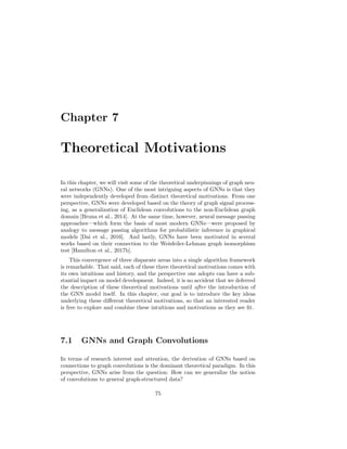
![Chapter 7
Theoretical Motivations
In this chapter, we will visit some of the theoretical underpinnings of graph neu-
ral networks (GNNs). One of the most intriguing aspects of GNNs is that they
were independently developed from distinct theoretical motivations. From one
perspective, GNNs were developed based on the theory of graph signal process-
ing, as a generalization of Euclidean convolutions to the non-Euclidean graph
domain [Bruna et al., 2014]. At the same time, however, neural message passing
approaches—which form the basis of most modern GNNs—were proposed by
analogy to message passing algorithms for probabilistic inference in graphical
models [Dai et al., 2016]. And lastly, GNNs have been motivated in several
works based on their connection to the Weisfeiler-Lehman graph isomorphism
test [Hamilton et al., 2017b].
This convergence of three disparate areas into a single algorithm framework
is remarkable. That said, each of these three theoretical motivations comes with
its own intuitions and history, and the perspective one adopts can have a sub-
stantial impact on model development. Indeed, it is no accident that we deferred
the description of these theoretical motivations until after the introduction of
the GNN model itself. In this chapter, our goal is to introduce the key ideas
underlying these different theoretical motivations, so that an interested reader
is free to explore and combine these intuitions and motivations as they see fit.
7.1 GNNs and Graph Convolutions
In terms of research interest and attention, the derivation of GNNs based on
connections to graph convolutions is the dominant theoretical paradigm. In this
perspective, GNNs arise from the question: How can we generalize the notion
of convolutions to general graph-structured data?
75](https://image.slidesharecdn.com/grlbook-210914153141/85/Grl-book-84-320.jpg)
![7.1. GNNS AND GRAPH CONVOLUTIONS 77
and its Fourier transform are real-valued, we can interpret the sequence
[s0, s1, ..., sN−1] as the coefficients of a Fourier series. In this view, sk tells
us the amplitude of the complex sinusoidal component e− i2π
N k
, which has
frequency 2πk
N (in radians). Often we will discuss high-frequency components
that have a large k and vary quickly as well as low-frequency components
that have k N and vary more slowly. This notion of low and high
frequency components will also have an analog in the graph domain, where
we will consider signals propagating between nodes in the graph.
In terms of signal processing, we can view the discrete convolution f ?h as a
filtering operation of the series (f(x1), f(x2), ..., f(xN )) by a filter h. Generally,
we view the series as corresponding to the values of the signal throughout time,
and the convolution operator applies some filter (e.g., a band-pass filter) to
modulate this time-varying signal.
One critical property of convolutions, which we will rely on below, is the fact
that they are translation (or shift) equivariant:
f(t + a) ? g(t) = f(t) ? g(t + a) = (f ? g)(t + a). (7.8)
This property means that translating a signal and then convolving it by a filter
is equivalent to convolving the signal and then translating the result. Note that
as a corollary convolutions are also equivariant to the difference operation:
∆f(t) ? g(t) = f(t) ? ∆g(t) = ∆(f ? g)(t), (7.9)
where
∆f(t) = f(t + 1) − f(t) (7.10)
is the Laplace (i.e., difference) operator on discrete univariate signals.
These notions of filtering and translation equivariance are central to digital
signal processing (DSP) and also underlie the intuition of convolutional neu-
ral networks (CNNs), which utilize a discrete convolution on two-dimensional
data. We will not attempt to cover even a small fraction of the fields of digital
signal processing, Fourier analysis, and harmonic analysis here, and we point
the reader to various textbooks on these subjects [Grafakos, 2004, Katznelson,
2004, Oppenheim et al., 1999, Rabiner and Gold, 1975].
7.1.2 From Time Signals to Graph Signals
In the previous section, we (briefly) introduced the notions of filtering and con-
volutions with respect to discrete time-varying signals. We now discuss how we
can connect discrete time-varying signals with signals on a graph. Suppose we
have a discrete time-varying signal f(t0), f(t2), ..., f(tN−1). One way of viewing
this signal is as corresponding to a chain (or cycle) graph (Figure 7.1), where
each point in time t is represented as a node and each function value f(t) rep-
resents the signal value at that time/node. Taking this view, it is convenient to
represent the signal as a vector f ∈ RN
, with each dimension corresponding to](https://image.slidesharecdn.com/grlbook-210914153141/85/Grl-book-86-320.jpg)
![78 CHAPTER 7. THEORETICAL MOTIVATIONS
0
…
1 N-2 N-1
Figure 7.1: Representation of a (cyclic) time-series as a chain graph.
a different node in the chain graph. In other words, we have that f[t] = f(t)
(as a slight abuse of notation). The edges in the graph thus represent how the
signal propagates; i.e., the signal propagates forward in time.2
One interesting aspect of viewing a time-varying signal as a chain graph is
that we can represent operations, such as time-shifts, using the adjacency and
Laplacian matrices of the graph. In particular, the adjacency matrix for this
chain graph corresponds to the circulant matrix Ac with
Ac[i, j] =
(
1 if j = (i + 1)mod N
0 otherwise,
(7.11)
and the (unnormalized) Laplacian Lc for this graph can be defined as
Lc = I − Ac. (7.12)
We can then represent time shifts as multiplications by the adjacency matrix,
(Acf)[t] = f[(t + 1)mod N ], (7.13)
and the difference operation by multiplication by the Laplacian,
(Lcf)[t] = f[t] − f[(t + 1)mod N ]. (7.14)
In this way, we can see that there is a close connection between the adjacency
and Laplacian matrices of a graph, and the notions of shifts and differences
for a signal. Multiplying a signal by the adjacency matrix propagates signals
from node to node, and multiplication by the Laplacian computes the difference
between a signal at each node and its immediate neighbors.
Given this graph-based view of transforming signals through matrix multi-
plication, we can similarly represent convolution by a filter h as matrix multi-
plication on the vector f:
(f ? h)(t) =
N−1
X
τ=0
f(τ)h(τ − t) (7.15)
= Qhf, (7.16)
2Note that we add a connection between the last and first nodes in the chain as a boundary
condition to keep the domain finite.](https://image.slidesharecdn.com/grlbook-210914153141/85/Grl-book-87-320.jpg)
![7.1. GNNS AND GRAPH CONVOLUTIONS 79
where Qh ∈ RN×N
is a matrix representation of the convolution operation by
filter function h and f = [f(t0), f(t2), ..., f(tN−1)]
is a vector representation
of the function f. Thus, in this view, we consider convolutions that can be
represented as a matrix transformation of the signal at each node in the graph.3
Of course, to have the equality between Equation (7.15) and Equation (7.16),
the matrix Qh must have some specific properties. In particular, we require
that multiplication by this matrix satisfies translation equivariance, which cor-
responds to commutativity with the circulant adjacency matrix Ac, i.e., we
require that
AcQh = QhAc. (7.17)
The equivariance to the difference operator is similarly defined as
LcQh = QhLc. (7.18)
It can be shown that these requirements are satisfied for a real matrix Qh if
Qh = pN (Ac) =
N−1
X
i=0
αiAi
c, (7.19)
i.e., if Qh is a polynomial function of the adjacency matrix Ac. In digital signal
processing terms, this is equivalent to the idea of representing general filters as
polynomial functions of the shift operator [Ortega et al., 2018].4
Generalizing to general graphs
We have now seen how shifts and convolutions on time-varying discrete signals
can be represented based on the adjacency matrix and Laplacian matrix of a
chain graph. Given this view, we can easily generalize these notions to more
general graphs.
In particular, we saw that a time-varying discrete signal corresponds to a
chain graph and that the notion of translation/difference equivariance corre-
sponds to a commutativity property with adjacency/Laplacian of this chain
graph. Thus, we can generalize these notions beyond the chain graph by con-
sidering arbitrary adjacency matrices and Laplacians. While the signal simply
propagates forward in time in a chain graph, in an arbitrary graph we might have
multiple nodes propagating signals to each other, depending on the structure of
the adjacency matrix. Based on this idea, we can define convolutional filters on
general graphs as matrices Qh that commute with the adjacency matrix or the
Laplacian.
More precisely, for an arbitrary graph with adjacency matrix A, we can
represent convolutional filters as matrices of the following form:
Qh = α0I + α1A + α2A2
+ ... + αN AN
. (7.20)
3This assumes a real-valued filter h.
4Note, however, that there are certain convolutional filters (e.g., complex-valued filters)
that cannot be represented in this way.](https://image.slidesharecdn.com/grlbook-210914153141/85/Grl-book-88-320.jpg)
![80 CHAPTER 7. THEORETICAL MOTIVATIONS
Intuitively, this gives us a spatial construction of a convolutional filter on graphs.
In particular, if we multiply a node feature vector x ∈ R|V |
by such a convolution
matrix Qh, then we get
Qhx = α0Ix + α1Ax + α2A2
x + ... + αN AN
x, (7.21)
which means that the convolved signal Qhx[u] at each node u ∈ V will corre-
spond to some mixture of the information in the node’s N-hop neighborhood,
with the α0, ..., αN terms controlling the strength of the information coming
from different hops.
We can easily generalize this notion of a graph convolution to higher dimen-
sional node features. If we have a matrix of node features X ∈ R|V|×m
then we
can similarly apply the convolutional filter as
QhX = α0IX + α1AX + α2A2
X + ... + αN AN
X. (7.22)
From a signal processing perspective, we can view the different dimensions of
the node features as different “channels”.
Graph convolutions and message passing GNNs
Equation (7.22) also reveals the connection between the message passing GNN
model we introduced in Chapter 5 and graph convolutions. For example, in the
basic GNN approach (see Equation 6.5) each layer of message passing essentially
corresponds to an application of the simple convolutional filter
Qh = I + A (7.23)
combined with some learnable weight matrices and a non-linearity. In general,
each layer of message passing GNN architecture aggregates information from
a node’s local neighborhood and combines this information with the node’s
current representation (see Equation 5.4). We can view these message passing
layers as a generalization of the simple linear filter in Equation (7.23), where we
use more complex non-linear functions. Moreover, by stacking multiple message
passing layers, GNNs are able to implicitly operate on higher order polynomials
of the adjacency matrix.
The adjacency matrix, Laplacian, or a normalized variant? In
Equation (7.22) we defined a convolution matrix Qh for arbitrary graphs
as a polynomial of the adjacency matrix. Defining Qh in this way guar-
antees that our filter commutes with the adjacency matrix, satisfying a
generalized notion of translation equivariance. However, in general com-
mutativity with the adjacency matrix (i.e., translation equivariance) does
not necessarily imply commutativity with the Laplacian L = D−A (or any
of its normalized variants). In this special case of the chain graph, we were
able to define filter matrices Qh that simultaneously commute with both
A and L, but for more general graphs we have a choice to make in terms](https://image.slidesharecdn.com/grlbook-210914153141/85/Grl-book-89-320.jpg)
![7.1. GNNS AND GRAPH CONVOLUTIONS 81
of whether we define convolutions based on the adjacency matrix or some
version of the Laplacian. Generally, there is no “right” decision in this case,
and there can be empirical trade-offs depending on the choice that is made.
Understanding the theoretical underpinnings of these trade-offs is an open
area of research [Ortega et al., 2018].
In practice researchers often use the symmetric normalized Laplacian
Lsym = D− 1
2 LD− 1
2 or the symmetric normalized adjacency matrix Asym =
D− 1
2 AD− 1
2 to define convolutional filters. There are two reasons why these
symmetric normalized matrices are desirable. First, both these matrices
have bounded spectrums, which gives them desirable numerical stability
properties. In addition—and perhaps more importantly—these two ma-
trices are simultaneously diagonalizable, which means that they share the
same eigenvectors. In fact, one can easily verify that there is a simple
relationship between their eigendecompositions, since
Lsym = I − Asym
⇒
Lsym = UΛU
Asym = U(I − Λ)U
, (7.24)
where U is the shared set of eigenvectors and Λ is the diagonal matrix
containing the Laplacian eigenvalues. This means that defining filters based
on one of these matrices implies commutativity with the other, which is a
very convenient and desirable property.
7.1.3 Spectral Graph Convolutions
We have seen how to generalize the notion of a signal and a convolution to the
graph domain. We did so by analogy to some important properties of discrete
convolutions (e.g., translation equivariance), and this discussion led us to the
idea of representing graph convolutions as polynomials of the adjacency matrix
(or the Laplacian). However, one key property of convolutions that we ignored
in the previous subsection is the relationship between convolutions and the
Fourier transform. In this section, we will thus consider the notion of a spectral
convolution on graphs, where we construct graph convolutions via an extension
of the Fourier transform to graphs. We will see that this spectral perspective
recovers many of the same results we previously discussed, while also revealing
some more general notions of a graph convolution.
The Fourier transform and the Laplace operator
To motivate the generalization of the Fourier transform to graphs, we rely on
the connection between the Fourier transform and the Laplace (i.e., difference)
operator. We previously saw a definition of the Laplace operator ∆ in the case
of a simple discrete time-varying signal (Equation 7.10) but this operator can](https://image.slidesharecdn.com/grlbook-210914153141/85/Grl-book-90-320.jpg)
![82 CHAPTER 7. THEORETICAL MOTIVATIONS
be generalized to apply to arbitrary smooth functions f : Rd
→ R as
∆f(x) = ∇2
f(x) (7.25)
=
n
X
i=1
∂2
f
∂x2
. (7.26)
This operator computes the divergence ∇ of the gradient ∇f(x). Intuitively, the
Laplace operator tells us the average difference between the function value at a
point and function values in the neighboring regions surrounding this point.
In the discrete time setting, the Laplace operator simply corresponds to the
difference operator (i.e., the difference between consecutive time points). In
the setting of general discrete graphs, this notion corresponds to the Laplacian,
since by definition
(Lx)[i] =
X
j∈V
A[i, j](x[i] − x[j]), (7.27)
which measures the difference between the value of some signal x[i] at a node
i and the signal values of all of its neighbors. In this way, we can view the
Laplacian matrix as a discrete analog of the Laplace operator, since it allows us
to quantify the difference between the value at a node and the values at that
node’s neighbors.
Now, an extremely important property of the Laplace operator is that its
eigenfunctions correspond to the complex exponentials. That is,
− ∆(e2πist
) = −
∂2
(e2πist
)
∂t2
= (2πs)2
e2πist
, (7.28)
so the eigenfunctions of ∆ are the same complex exponentials that make up
the modes of the frequency domain in the Fourier transform (i.e., the sinu-
soidal plane waves), with the corresponding eigenvalue indicating the frequency.
In fact, one can even verify that the eigenvectors u1, ..., un of the circulant
Laplacian Lc ∈ Rn×n
for the chain graph are uj = 1
√
n
[1, ωj, ω2
j , ..., ωn
j ] where
ωj = e
2πj
n .
The graph Fourier transform
The connection between the eigenfunctions of the Laplace operator and the
Fourier transform allows us to generalize the Fourier transform to arbitrary
graphs. In particular, we can generalize the notion of a Fourier transform by
considering the eigendecomposition of the general graph Laplacian:
L = UΛU
, (7.29)
where we define the eigenvectors U to be the graph Fourier modes, as a graph-
based notion of Fourier modes. The matrix Λ is assumed to have the correspond-
ing eigenvalues along the diagonal, and these eigenvalues provide a graph-based
notion of different frequency values. In other words, since the eigenfunctions of](https://image.slidesharecdn.com/grlbook-210914153141/85/Grl-book-91-320.jpg)
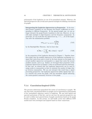
2
(7.38)
by the properties of the Laplacian discussed in Chapter 1. Together these
facts imply that the smallest eigenvector of the Laplacian corresponds to a
signal that varies from node to node by the least amount on the graph, the
second smallest eigenvector corresponds to a signal that varies the second
smallest amount, and so on. Indeed, we leveraged these properties of the
Laplacian eigenvectors in Chapter 1 when we performed spectral clustering.
In that case, we showed that the Laplacian eigenvectors can be used to
assign nodes to communities so that we minimize the number of edges that
go between communities. We can now interpret this result from a signal
processing perspective: the Laplacian eigenvectors define signals that vary
in a smooth way across the graph, with the smoothest signals indicating
the coarse-grained community structure of the graph.
7.1.4 Convolution-Inspired GNNs
The previous subsections generalized the notion of convolutions to graphs. We
saw that basic convolutional filters on graphs can be represented as polynomials
of the (normalized) adjacency matrix or Laplacian. We saw both spatial and
spectral motivations of this fact, and we saw how the spectral perspective can
be used to define more general forms of graph convolutions based on the graph
Fourier transform. In this section, we will briefly review how different GNN
models have been developed and inspired based on these connections.](https://image.slidesharecdn.com/grlbook-210914153141/85/Grl-book-93-320.jpg)
![7.1. GNNS AND GRAPH CONVOLUTIONS 85
Purely convolutional approaches
Some of the earliest work on GNNs can be directly mapped to the graph convo-
lution definitions of the previous subsections. The key idea in these approaches
is that they use either Equation (7.34) or Equation (7.35) to define a convo-
lutional layer, and a full model is defined by stacking and combining multiple
convolutional layers with non-linearities. For example, in early work Bruna
et al. [2014] experimented with the non-parametric spectral filter (Equation
7.34) as well as a parametric spectral filter (Equation 7.35), where they defined
the polynomial pN (Λ) via a cubic spline approach. Following on this work,
Defferrard et al. [2016] defined convolutions based on Equation 7.35 and defined
pN (L) using Chebyshev polynomials. This approach benefits from the fact that
Chebyshev polynomials have an efficient recursive formulation and have various
properties that make them suitable for polynomial approximation [Mason and
Handscomb, 2002]. In a related approach, Liao et al. [2019b] learn polynomials
of the Laplacian based on the Lanczos algorithm.
There are also approaches that go beyond real-valued polynomials of the
Laplacian (or the adjacency matrix). For example, Levie et al. [2018] consider
Cayley polynomials of the Laplacian and Bianchi et al. [2019] consider ARMA
filters. Both of these approaches employ more general parametric rational com-
plex functions of the Laplacian (or the adjacency matrix).
Graph convolutional networks and connections to message passing
In their seminal work, Kipf and Welling [2016a] built off the notion of graph
convolutions to define one of the most popular GNN architectures, commonly
known as the graph convolutional network (GCN). The key insight of the GCN
approach is that we can build powerful models by stacking very simple graph
convolutional layers. A basic GCN layer is defined in Kipf and Welling [2016a]
as
H(k)
= σ
ÃH(k−1)
W(k)
, (7.39)
where à = (D+I)− 1
2 (I+A)(D+I)− 1
2 is a normalized variant of the adjacency
matrix (with self-loops) and W(k)
is a learnable parameter matrix. This model
was initially motivated as a combination of a simple graph convolution (based
on the polynomial I + A), with a learnable weight matrix, and a non-linearity.
As discussed in Chapter 5 we can also interpret the GCN model as a vari-
ation of the basic GNN message passing approach. In general, if we consider
combining a simple graph convolution defined via the polynomial I + A with
non-linearities and trainable weight matrices we recover the basic GNN:
H(k)
= σ
AH(k−1)
W
(k)
neigh + H(k−1)
W
(k)
self
. (7.40)
In other words, a simple graph convolution based on I + A is equivalent to
aggregating information from neighbors and combining that with information](https://image.slidesharecdn.com/grlbook-210914153141/85/Grl-book-94-320.jpg)
![86 CHAPTER 7. THEORETICAL MOTIVATIONS
from the node itself. Thus we can view the notion of message passing as cor-
responding to a simple form of graph convolutions combined with additional
trainable weights and non-linearities.
Over-smoothing as a low-pass convolutional filter In Chapter 5 we
introduced the problem of over-smoothing in GNNs. The intuitive idea
in over-smoothing is that after too many rounds of message passing, the
embeddings for all nodes begin to look identical and are relatively unin-
formative. Based on the connection between message-passing GNNs and
graph convolutions, we can now understand over-smoothing from the per-
spective of graph signal processing.
The key intuition is that stacking multiple rounds of message passing in
a basic GNN is analogous to applying a low-pass convolutional filter, which
produces a smoothed version of the input signal on the graph. In particular,
suppose we simplify a basic GNN (Equation 7.40) to the following update
equation:
H(k)
= AsymH(k−1)
W(k)
. (7.41)
Compared to the basic GNN in Equation (7.40), we have simplified the
model by removing the non-linearity and removing addition of the “self”
embeddings at each message-passing step. For mathematical simplicity
and numerical stability, we will also assume that we are using the sym-
metric normalized adjacency matrix Asym = D− 1
2 AD− 1
2 rather than the
unnormalized adjacency matrix. This model is similar to the simple GCN
approach proposed in Kipf and Welling [2016a] and essentially amounts to
taking the average over the neighbor embeddings at each round of message
passing.
Now, it is easy to see that after K rounds of message passing based on
Equation (7.41), we will end up with a representation that depends on the
Kth power of the adjacency matrix:
H(K)
= AK
symXW, (7.42)
where W is some linear operator and X is the matrix of input node features.
To understand the connection between over-smoothing and convolutional
filters, we just need to recognize that the multiplication AK
symX of the input
node features by a high power of the adjacency matrix can be interpreted
as convolutional filter based on the lowest-frequency signals of the graph
Laplacian.
For example, suppose we use a large enough value of K such that we
have reached the a fixed point of the following recurrence:
AsymH(K)
= H(K)
. (7.43)
One can verify that this fixed point is attainable when using the normalized
adjacency matrix, since the dominant eigenvalue of Asym is equal to one.](https://image.slidesharecdn.com/grlbook-210914153141/85/Grl-book-95-320.jpg)
![7.1. GNNS AND GRAPH CONVOLUTIONS 87
We can see that at this fixed point, all the node features will have converged
to be completely defined by the dominant eigenvector of Asym, and more
generally, higher powers of Asym will emphasize the largest eigenvalues
of this matrix. Moreover, we know that the largest eigenvalues of Asym
correspond to the smallest eigenvalues of its counterpart, the symmetric
normalized Laplacian Lsym (e.g., see Equation 7.24). Together, these facts
imply that multiplying a signal by high powers of Asym corresponds to a
convolutional filter based on the lowest eigenvalues (or frequencies) of Lsym,
i.e., it produces a low-pass filter!
Thus, we can see from this simplified model that stacking many rounds
of message passing leads to convolutional filters that are low-pass, and—in
the worst case—these filters simply converge all the node representations
to constant values within connected components on the graph (i.e., the
“zero-frequency” of the Laplacian).
Of course, in practice we use more complicated forms of message pass-
ing, and this issue is partially alleviated by including each node’s previous
embedding in the message-passing update step. Nonetheless, it is instruc-
tive to understand how stacking “deeper” convolutions on graphs in a naive
way can actually lead to simpler, rather than more complex, convolutional
filters.
GNNs without message passing
Inspired by connections to graph convolutions, several recent works have also
proposed to simplify GNNs by removing the iterative message passing process.
In these approaches, the models are generally defined as
Z = MLPθ (f(A)MLPφ(X)) , (7.44)
where f : RV|×|V|
→ RV|×|V|
is some deterministic function of the adjacency ma-
trix A, MLP denotes a dense neural network, X ∈ R|V|×m
is the matrix of input
node features, and Z ∈ R|V|×d
is the matrix of learned node representations.
For example, in Wu et al. [2019], they define
f(A) = Ãk
, (7.45)
where à = (D + I)− 1
2 (A + I)(D + I)− 1
2 is the symmetric normalized adjacency
matrix (with self-loops added). In a closely related work Klicpera et al. [2019]
defines f by analogy to the personalized PageRank algorithm as5
f(A) = α(I − (1 − α)Ã)−1
(7.46)
= α
∞
X
k=0
I − αÃ
k
. (7.47)
5Note that the equality between Equations (7.46) and (7.47) requires that the dominant
eigenvalue of (I − αA) is bounded above by 1. In practice, Klicpera et al. [2019] use power
iteration to approximate the inversion in Equation (7.46).](https://image.slidesharecdn.com/grlbook-210914153141/85/Grl-book-96-320.jpg)
![88 CHAPTER 7. THEORETICAL MOTIVATIONS
The intuition behind these approaches is that we often do not need to interleave
trainable neural networks with graph convolution layers. Instead, we can simply
use neural networks to learn feature transformations at the beginning and end
of the model and apply a deterministic convolution layer to leverage the graph
structure. These simple models are able to outperform more heavily parameter-
ized message passing models (e.g., GATs or GraphSAGE) on many classification
benchmarks.
There is also increasing evidence that using the symmetric normalized ad-
jacency matrix with self-loops leads to effective graph convolutions, especially
in this simplified setting without message passing. Both Wu et al. [2019] and
Klicpera et al. [2019] found that convolutions based on à achieved the best em-
pirical performance. Wu et al. [2019] also provide theoretical support for these
results. They prove that adding self-loops shrinks the spectrum of corresponding
graph Laplacian by reducing the magnitude of the dominant eigenvalue. Intu-
itively, adding self-loops decreases the influence of far-away nodes and makes
the filtered signal more dependent on local neighborhoods on the graph.
7.2 GNNs and Probabilistic Graphical Models
GNNs are well-understood and well-motivated as extensions of convolutions to
graph-structured data. However, there are alternative theoretical motivations
for the GNN framework that can provide interesting and novel perspectives.
One prominent example is the motivation of GNNs based on connections to
variational inference in probabilistic graphical models (PGMs).
In this probabilistic perspective, we view the embeddings zu, ∀u ∈ V for
each node as latent variables that we are attempting to infer. We assume that
we observe the graph structure (i.e., the adjacency matrix, A) and the input
node features, X, and our goal is to infer the underlying latent variables (i.e.,
the embeddings zv) that can explain this observed data. The message passing
operation that underlies GNNs can then be viewed as a neural network analogue
of certain message passing algorithms that are commonly used for variational
inference to infer distributions over latent variables. This connection was first
noted by Dai et al. [2016], and much of the proceeding discussions is based
closely on their work.
Note that the presentation in this section assumes a substantial background
in PGMs, and we recommend Wainwright and Jordan [2008] as a good resource
for the interested reader. However, we hope and expect that even a reader
without any knowledge of PGMS can glean useful insights from the following
discussions.
7.2.1 Hilbert Space Embeddings of Distributions
To understand the connection between GNNs and probabilistic inference, we
first (briefly) introduce the notion of embedding distributions in Hilbert spaces
[Smola et al., 2007]. Let p(x) denote a probability density function defined](https://image.slidesharecdn.com/grlbook-210914153141/85/Grl-book-97-320.jpg)
![7.2. GNNS AND PROBABILISTIC GRAPHICAL MODELS 89
over the random variable x ∈ Rm
. Given an arbitrary (and possibly infinite
dimensional) feature map φ : Rm
→ R, we can represent the density p(x)
based on its expected value under this feature map:
µx =
Z
Rm
φ(x)p(x)dx. (7.48)
The key idea with Hilbert space embeddings of distributions is that Equation
(7.48) will be injective, as long as a suitable feature map φ is used. This means
that µx can serve as a sufficient statistic for p(x), and any computations we
want to perform on p(x) can be equivalently represented as functions of the
embedding µx. A well-known example of a feature map that would guarantee
this injective property is the feature map induced by the Gaussian radial basis
function (RBF) kernel [Smola et al., 2007].
The study of Hilbert space embeddings of distributions is a rich area of
statistics. In the context of the connection to GNNs, however, the key takeaway
is simply that we can represent distributions p(x) as embeddings µx in some
feature space. We will use this notion to motivate the GNN message passing
algorithm as a way of learning embeddings that represent the distribution over
node latents p(zv).
7.2.2 Graphs as Graphical Models
Taking a probabilistic view of graph data, we can assume that the graph struc-
ture we are given defines the dependencies between the different nodes. Of
course, we usually interpret graph data in this way. Nodes that are connected
in a graph are generally assumed to be related in some way. However, in the
probabilistic setting, we view this notion of dependence between nodes in a
formal, probabilistic way.
To be precise, we say that a graph G = (V, E) defines a Markov random field:
p({xv}, {zv}) ∝
Y
v∈V
Φ(xv, zv)
Y
(u,v)∈E
Ψ(zu, zv), (7.49)
where Φ and Ψ are non-negative potential functions, and where we use {xv} as
a shorthand for the set {xv, ∀v ∈ V}. Equation (7.49) says that the distribution
p({xv}, {zv}) over node features and node embeddings factorizes according to
the graph structure. Intuitively, Φ(xv, zv) indicates the likelihood of a node
feature vector xv given its latent node embedding zv, while Ψ controls the de-
pendency between connected nodes. We thus assume that node features are
determined by their latent embeddings, and we assume that the latent embed-
dings for connected nodes are dependent on each other (e.g., connected nodes
might have similar embeddings).
In the standard probabilistic modeling setting, Φ and Ψ are usually defined
as parametric functions based on domain knowledge, and, most often, these
functions are assumed to come from the exponential family to ensure tractability
[Wainwright and Jordan, 2008]. In our presentation, however, we are agnostic to](https://image.slidesharecdn.com/grlbook-210914153141/85/Grl-book-98-320.jpg)
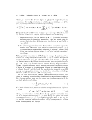
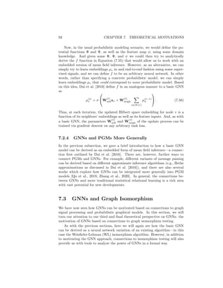
![92 CHAPTER 7. THEORETICAL MOTIVATIONS
Now, in the usual probabilistic modeling scenario, we would define the po-
tential functions Φ and Ψ, as well as the feature map φ, using some domain
knowledge. And given some Φ, Ψ, and ψ we could then try to analytically
derive the f function in Equation (7.55) that would allow us to work with an
embedded version of mean field inference. However, as an alternative, we can
simply try to learn embeddings µv in and end-to-end fashion using some super-
vised signals, and we can define f to be an arbitrary neural network. In other
words, rather than specifying a concrete probabilistic model, we can simply
learn embeddings µv that could correspond to some probabilistic model. Based
on this idea, Dai et al. [2016] define f in an analogous manner to a basic GNN
as
µ(t)
v = σ
W
(t)
selfxv + W
(t)
neigh
X
u∈N (v)
µ(t−1)
u
. (7.56)
Thus, at each iteration, the updated Hilbert space embedding for node v is a
function of its neighbors’ embeddings as well as its feature inputs. And, as with
a basic GNN, the parameters W
(t)
self and W
(t)
neigh of the update process can be
trained via gradient descent on any arbitrary task loss.
7.2.4 GNNs and PGMs More Generally
In the previous subsection, we gave a brief introduction to how a basic GNN
model can be derived as an embedded form of mean field inference—a connec-
tion first outlined by Dai et al. [2016]. There are, however, further ways to
connect PGMs and GNNs. For example, different variants of message passing
can be derived based on different approximate inference algorithms (e.g., Bethe
approximations as discussed in Dai et al. [2016]), and there are also several
works which explore how GNNs can be integrated more generally into PGM
models [Qu et al., 2019, Zhang et al., 2020]. In general, the connections be-
tween GNNs and more traditional statistical relational learning is a rich area
with vast potential for new developments.
7.3 GNNs and Graph Isomorphism
We have now seen how GNNs can be motivated based on connections to graph
signal processing and probabilistic graphical models. In this section, we will
turn our attention to our third and final theoretical perspective on GNNs: the
motivation of GNNs based on connections to graph isomorphism testing.
As with the previous sections, here we will again see how the basic GNN
can be derived as a neural network variation of an existing algorithm—in this
case the Weisfieler-Lehman (WL) isomorphism algorithm. However, in addition
to motivating the GNN approach, connections to isomorphism testing will also
provide us with tools to analyze the power of GNNs in a formal way.](https://image.slidesharecdn.com/grlbook-210914153141/85/Grl-book-101-320.jpg)
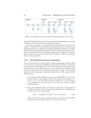
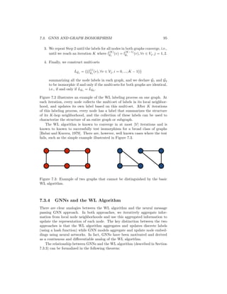
![7.3. GNNS AND GRAPH ISOMORPHISM 95
3. We repeat Step 2 until the labels for all nodes in both graphs converge, i.e.,
until we reach an iteration K where l
(K)
Gj
(v) = l
(K−1)
Gi
(v), ∀v ∈ Vj, j = 1, 2.
4. Finally, we construct multi-sets
LGj
= {{l
(i)
Gj
(v), ∀v ∈ Vj, i = 0, ..., K − 1}}
summarizing all the node labels in each graph, and we declare G1 and G2
to be isomorphic if and only if the multi-sets for both graphs are identical,
i.e., if and only if LG1 = LG2 .
Figure 7.2 illustrates an example of the WL labeling process on one graph. At
each iteration, every node collects the multi-set of labels in its local neighbor-
hood, and updates its own label based on this multi-set. After K iterations
of this labeling process, every node has a label that summarizes the structure
of its K-hop neighborhood, and the collection of these labels can be used to
characterize the structure of an entire graph or subgraph.
The WL algorithm is known to converge in at most |V| iterations and is
known to known to successfully test isomorphism for a broad class of graphs
[Babai and Kucera, 1979]. There are, however, well known cases where the test
fails, such as the simple example illustrated in Figure 7.3.
Figure 7.3: Example of two graphs that cannot be distinguished by the basic
WL algorithm.
7.3.4 GNNs and the WL Algorithm
There are clear analogies between the WL algorithm and the neural message
passing GNN approach. In both approaches, we iteratively aggregate infor-
mation from local node neighborhoods and use this aggregated information to
update the representation of each node. The key distinction between the two
approaches is that the WL algorithm aggregates and updates discrete labels
(using a hash function) while GNN models aggregate and update node embed-
dings using neural networks. In fact, GNNs have been motivated and derived
as a continuous and differentiable analog of the WL algorithm.
The relationship between GNNs and the WL algorithm (described in Section
7.3.3) can be formalized in the following theorem:](https://image.slidesharecdn.com/grlbook-210914153141/85/Grl-book-104-320.jpg)
![96 CHAPTER 7. THEORETICAL MOTIVATIONS
Theorem 4 ([Morris et al., 2019, Xu et al., 2019]). Define a message-passing
GNN (MP-GNN) to be any GNN that consists of K message-passing layers of
the following form:
h(k+1)
u = UPDATE
(k)
h(k)
u , AGGREGATE
(k)
({h(k)
v , ∀v ∈ N(u)})
, (7.61)
where AGGREGATE is a differentiable permutation invariant function and UPDATE
is a differentiable function. Further, suppose that we have only discrete feature
inputs at the initial layer, i.e., h
(0)
u = xu ∈ Zd
, ∀u ∈ V. Then we have that
h
(K)
u 6= h
(K)
v only if the nodes u and v have different labels after K iterations
of the WL algorithm.
In intuitive terms, Theorem 7.3.4 states that GNNs are no more powerful than
the WL algorithm when we have discrete information as node features. If the WL
algorithm assigns the same label to two nodes, then any message-passing GNN
will also assign the same embedding to these two nodes. This result on node
labeling also extends to isomorphism testing. If the WL test cannot distinguish
between two graphs, then a MP-GNN is also incapable of distinguishing between
these two graphs. We can also show a more positive result in the other direction:
Theorem 5 ([Morris et al., 2019, Xu et al., 2019]). There exists a MP-GNN
such that h
(K)
u = h
(K)
v if and only if the two nodes u and v have the same label
after K iterations of the WL algorithm.
This theorem states that there exist message-passing GNNs that are as powerful
as the WL test.
Which MP-GNNs are most powerful? The two theorems above state
that message-passing GNNs are at most as powerful as the WL algorithm
and that there exist message-passing GNNs that are as powerful as the WL
algorithm. So which GNNs actually obtain this theoretical upper bound?
Interestingly, the basic GNN that we introduced at the beginning of Chap-
ter 5 is sufficient to satisfy this theory. In particular, if we define the
message passing updates as follows:
h(k)
u = σ
W
(k)
selfh(k−1)
u + W
(k)
neigh
X
v∈N (u)
h(k−1)
v + b(k)
, (7.62)
then this GNN is sufficient to match the power of the WL algorithm [Morris
et al., 2019].
However, most of the other GNN models discussed in Chapter 5 are
not as powerful as the WL algorithm. Formally, to be as powerful as the
WL algorithm, the AGGREGATE and UPDATE functions need to be injective
[Xu et al., 2019]. This means that the AGGREGATE and UPDATE operators
need to be map every unique input to a unique output value, which is not
the case for many of the models we discussed. For example, AGGREGATE
functions that use a (weighted) average of the neighbor embeddings are not](https://image.slidesharecdn.com/grlbook-210914153141/85/Grl-book-105-320.jpg)
![7.3. GNNS AND GRAPH ISOMORPHISM 97
injective; if all the neighbors have the same embedding then a (weighted)
average will not be able to distinguish between input sets of different sizes.
Xu et al. [2019] provide a detailed discussion of the relative power of
various GNN architectures. They also define a “minimal” GNN model,
which has few parameters but is still as powerful as the WL algorithm.
They term this model the Graph Isomorphism Network (GIN), and it is
defined by the following update:
h(k)
u = MLP(k)
(1 + (k)
)h(k−1)
u +
X
v∈N (u)
h(k−1)
v
, (7.63)
where (k)
is a trainable parameter.
7.3.5 Beyond the WL Algorithm
The previous subsection highlighted an important negative result regarding
message-passing GNNs (MP-GNNs): these models are no more powerful than
the WL algorithm. However, despite this negative result, investigating how we
can make GNNs that are provably more powerful than the WL algorithm is an
active area of research.
Relational pooling
One way to motivate provably more powerful GNNs is by considering the failure
cases of the WL algorithm. For example, we can see in Figure 7.3 that the WL
algorithm—and thus all MP-GNNs—cannot distinguish between a connected
6-cycle and a set of two triangles. From the perspective of message passing,
this limitation stems from the fact that AGGREGATE and UPDATE operations are
unable to detect when two nodes share a neighbor. In the example in Figure
7.3, each node can infer from the message passing operations that they have
two degree-2 neighbors, but this information is not sufficient to detect whether
a node’s neighbors are connected to one another. This limitation is not simply
a corner case illustrated in Figure 7.3. Message passing approaches generally
fail to identify closed triangles in a graph, which is a critical limitation.
To address this limitation, Murphy et al. [2019] consider augmenting MP-
GNNs with unique node ID features. If we use MP-GNN(A, X) to denote an
arbitrary MP-GNN on input adjacency matrix A and node features X, then
adding node IDs is equivalent to modifying the MP-GNN to the following:
MP-GNN(A, X ⊕ I), (7.64)
where I is the d × d-dimensional identity matrix and ⊕ denotes column-wise
matrix concatenation. In other words, we simply add a unique, one-hot indicator
feature for each node. In the case of Figure 7.3, adding unique node IDs would](https://image.slidesharecdn.com/grlbook-210914153141/85/Grl-book-106-320.jpg)
![98 CHAPTER 7. THEORETICAL MOTIVATIONS
allow a MP-GNN to identify when two nodes share a neighbor, which would
make the two graphs distinguishable.
Unfortunately, however, this idea of adding node IDs does not solve the
problem. In fact, by adding unique node IDs we have actually introduced a
new and equally problematic issue: the MP-GNN is no longer permutation
equivariant. For a standard MP-GNN we have that
P(MP-GNN(A, X)) = MP-GNN(PAP
, PX), (7.65)
where P ∈ P is an arbitrary permutation matrix. This means that standard
MP-GNNs are permutation equivariant. If we permute the adjacency matrix
and node features, then the resulting node embeddings are simply permuted
in an equivalent way. However, MP-GNNs with node IDs are not permutation
invariant since in general
P(MP-GNN(A, X ⊕ I)) 6= MP-GNN(PAP
, (PX) ⊕ I). (7.66)
The key issue is that assigning a unique ID to each node fixes a particular node
ordering for the graph, which breaks the permutation equivariance.
To alleviate this issue, Murphy et al. [2019] propose the Relational Pooling
(RP) approach, which involves marginalizing over all possible node permuta-
tions. Given any MP-GNN the RP extension of this GNN is given by
RP-GNN(A, X) =
X
P∈P
MP-GNN(PAP
, (PX) ⊕ I). (7.67)
Summing over all possible permutation matrices P ∈ P recovers the permuta-
tion invariance, and we retain the extra representational power of adding unique
node IDs. In fact, Murphy et al. [2019] prove that the RP extension of a MP-
GNN can distinguish graphs that are indistinguishable by the WL algorithm.
The limitation of the RP approach is in its computational complexity. Naively
evaluating Equation (7.67) has a time complexity of O(|V|!), which is infeasible
in practice. Despite this limitation, however, Murphy et al. [2019] show that
the RP approach can achieve strong results using various approximations to
decrease the computation cost (e.g., sampling a subset of permutations).
The k-WL test and k-GNNs
The Relational Pooling (RP) approach discussed above can produce GNN mod-
els that are provably more powerful than the WL algorithm. However, the RP
approach has two key limitations:
1. The full algorithm is computationally intractable.
2. We know that RP-GNNs are more powerful than the WL test, but we
have no way to characterize how much more powerful they are.
To address these limitations, several approaches have considered improving
GNNs by adapting generalizations of the WL algorithm.](https://image.slidesharecdn.com/grlbook-210914153141/85/Grl-book-107-320.jpg)
![7.3. GNNS AND GRAPH ISOMORPHISM 99
The WL algorithm we introduced in Section 7.3.3 is in fact just the simplest
of what is known as the family of k-WL algorithms. In fact, the WL algorithm
we introduced previously is often referred to as the 1-WL algorithm, and it
can be generalized to the k-WL algorithm for k 1. The key idea behind the
k-WL algorithms is that we label subgraphs of size k rather than individual
nodes. The k-WL algorithm generates representation of a graph G through the
following steps:
1. Let s = (u1, u2, ..., uk) ∈ Vk
be a tuple defining a subgraph of size k, where
u1 6= u2 6= ... 6= uk. Define the initial label l
(0)
G (s) for each subgraph by
the isomorphism class of this subgraph (i.e., two subgraphs get the same
label if and only if they are isomorphic).
2. Next, we iteratively assign a new label to each subgraph by hashing the
multi-set of the current labels within this subgraph’s neighborhood:
l
(i)
G (s) = HASH({{l
(i−1)
G (s0
), ∀s0
∈ Nj(s), j = 1, ..., k}}, l
(i−1)
G (s)),
where the jth subgraph neighborhood is defined as
Nj(s) = {{(u1, ..., uj−1, v, uj+1, ..., uk), ∀v ∈ V}}. (7.68)
3. We repeat Step 2 until the labels for all subgraphs converge, i.e., until we
reach an iteration K where l
(K)
G (s) = l
(K−1)
G (s) for every k-tuple of nodes
s ∈ Vk
.
4. Finally, we construct a multi-set
LG = {{l
(i)
G (v), ∀s ∈ Vk
, i = 0, ..., K − 1}}
summarizing all the subgraph labels in the graph.
As with the 1-WL algorithm, the summary LG multi-set generated by the k-WL
algorithm can be used to test graph isomorphism by comparing the multi-sets
for two graphs. There are also graph kernel methods based on the k-WL test
[Morris et al., 2019], which are analogous to the WL-kernel introduced that was
in Chapter 1.
An important fact about the k-WL algorithm is that it introduces a hierarchy
of representational capacity. For any k ≥ 2 we have that the (k + 1)-WL test is
strictly more powerful than the k-WL test.6
Thus, a natural question to ask is
whether we can design GNNs that are as powerful as the k-WL test for k 2,
and, of course, a natural design principle would be to design GNNs by analogy
to the k-WL algorithm.
Morris et al. [2019] attempt exactly this: they develop a k-GNN approach
that is a differentiable and continuous analog of the k-WL algorithm. k-GNNs
6However, note that running the k-WL requires solving graph isomorphism for graphs
of size k, since Step 1 in the k-WL algorithm requires labeling graphs according to their
isomorphism type. Thus, running the k-WL for k 3 is generally computationally intractable.](https://image.slidesharecdn.com/grlbook-210914153141/85/Grl-book-108-320.jpg)
![100 CHAPTER 7. THEORETICAL MOTIVATIONS
learn embeddings associated with subgraphs—rather than nodes—and the mes-
sage passing occurs according to subgraph neighborhoods (e.g., as defined in
Equation 7.68). Morris et al. [2019] prove that k-GNNs can be as expressive as
the k-WL algorithm. However, there are also serious computational concerns for
both the k-WL test and k-GNNs, as the time complexity of the message passing
explodes combinatorially as k increases. These computational concerns necessi-
tate various approximations to make k-GNNs tractable in practice [Morris et al.,
2019].
Invariant and equivariant k-order GNNs
Another line of work that is motivated by the idea of building GNNs that are
as powerful as the k-WL test are the invariant and equivariant GNNs proposed
by Maron et al. [2019]. A crucial aspect of message-passing GNNs (MP-GNNs;
as defined in Theorem 7.3.4) is that they are equivariant to node permutations,
meaning that
P(MP-GNN(A, X)) = MP-GNN(PAP
, PX). (7.69)
for any permutation matrix P ∈ P. This equality says that that permuting the
input to an MP-GNN simply results in the matrix of output node embeddings
being permuted in an analogous way.
In addition to this notion of equivariance, we can also define a similar notion
of permutation invariance for MP-GNNs at the graph level. In particular, MP-
GNNs can be extended with a POOL : R|V|×d
→ R function (see Chapter 5),
which maps the matrix of learned node embeddings Z ∈ R|V|×d
to an embedding
zG ∈ Rd
of the entire graph. In this graph-level setting we have that MP-GNNs
are permutation invariant, i.e.
POOL MP-GNN(PAP
, PX)
= POOL (MP-GNN(A, X)) , (7.70)
meaning that the pooled graph-level embedding does not change when different
node orderings are used.
Based on this idea of invariance and equivariance, Maron et al. [2019] propose
a general form of GNN-like models based on permutation equivariant/invariant
tensor operations. Suppose we have an order-(k + 1) tensor X ∈ R|V|k
×d
, where
we assume that the first k channels/modes of this tensor are indexed by the
nodes of the graph. We use the notation P ? X to denote the operation where
we permute the first k channels of this tensor according the node permutation
matrix P. We can then define an linear equivariant layer as a linear operator
(i.e., a tensor) L : R|V|k1 ×d1
→ R|V|k2 ×d2
:
L × (P ? X) = P ? (L × X), ∀P ∈ P, (7.71)
where we use × to denote a generalized tensor product. Invariant linear opera-
tors can be similarly defined as tensors L that satisfy the following equality:
L × (P ? X) = L × X, ∀P ∈ P. (7.72)](https://image.slidesharecdn.com/grlbook-210914153141/85/Grl-book-109-320.jpg)
![7.3. GNNS AND GRAPH ISOMORPHISM 101
Note that both equivariant and invariant linear operators can be represented
as tensors, but they have different structure. In particular, an equivariant oper-
ator L : R|V|k
×d1
→ R|V|k
×d2
corresponds to a tensor L ∈ R|V|2k
×d1×d2
, which
has 2k channels indexed by nodes (i.e., twice as many node channels as the in-
put). On the other hand, an invariant operator L : R|V|k
×d1
→ Rd2
corresponds
to a tensor L ∈ R|V|k
×d1×d2
, which has k channels indexed by nodes (i.e., the
same number as the input). Interestingly, taking this tensor view of the linear
operators, the equivariant (Equation 7.71) and invariant (Equation 7.72) prop-
erties for can be combined into a single requirement that the L tensor is a fixed
point under node permutations:
P ? L = L, ∀P ∈ P. (7.73)
In other words, for a given input X ∈ R|V |k
×d
, both equivariant and invariant
linear operators on this input will correspond to tensors that satisfy the fixed
point in Equation (7.73), but the number of channels in the tensor will differ
depending on whether it is an equivariant or invariant operator.
Maron et al. [2019] show that tensors satisfying the the fixed point in Equa-
tion (7.73) can be constructed as a linear combination of a set of fixed basis
elements. In particular, any order-l tensor L that satisfies Equation (7.73) can
be written as
L = β1B1 + β2 + ... + βb(l)Bb(l), (7.74)
where Bi are a set of fixed basis tensors, βi ∈ R are real-valued weights, and b(l)
is the lth Bell number. The construction and derivation of these basis tensors
is mathematically involved and is closely related to the theory of Bell numbers
from combinatorics. However, a key fact and challenge is that the number of
basis tensors needed grows with lth Bell number, which is an exponentially
increasing series.
Using these linear equivariant and invariant layers, Maron et al. [2019] de-
fine their invariant k-order GNN model based on the following composition of
functions:
MLP ◦ L0 ◦ σ ◦ L1 ◦ σL2 · · · σ ◦ Lm × X. (7.75)
In this composition, we apply m equivariant linear layers L1, ..., Lm, where
Li : L : R|V|ki ×d1
→ R|V|ki+1 ×d2
with maxi ki = k and k1 = 2. Between each
of these linear equivariant layers an element-wise non-linearity, denoted by σ,
is applied. The penultimate function in the composition, is an invariant linear
layer, L0, which is followed by a multi-layer perceptron (MLP) as the final
function in the composition. The input to the k-order invariant GNN is the
tensor X ∈ R|V|2
×d
, where the first two channels correspond to the adjacency
matrix and the remaining channels encode the initial node features/labels.
This approach is called k-order because the equivariant linear layers involve
tensors that have up to k different channels. Most importantly, however, Maron
et al. [2019] prove that k-order models following Equation 7.75 are equally pow-
erful as the k-WL algorithm. As with the k-GNNs discussed in the previous
section, however, constructing k-order invariant models for k 3 is generally
computationally intractable.](https://image.slidesharecdn.com/grlbook-210914153141/85/Grl-book-110-320.jpg)
![Chapter 8
Traditional Graph
Generation Approaches
The previous parts of this book introduced a wide variety of methods for learning
representations of graphs. In this final part of the book, we will discuss a distinct
but closely related task: the problem of graph generation.
The goal of graph generation is to build models that can generate realistic
graph structures. In some ways, we can view this graph generation problem as
the mirror image of the graph embedding problem. Instead of assuming that
we are given a graph structure G = (V, E) as input to our model, in graph
generation we want the output of our model to be a graph G. Of course, simply
generating an arbitrary graph is not necessarily that challenging. For instance,
it is trivial to generate a fully connected graph or a graph with no edges. The key
challenge in graph generation, however, is generating graphs that have certain
desirable properties. As we will see in the following chapters, the way in which
we define “desirable properties”—and how we perform graph generation—varies
drastically between different approaches.
In this chapter, we begin with a discussion of traditional approaches to graph
generation. These tradiational approaches pre-date most research on graph
representation learning—and even machine learning research in general. The
methods we will discuss in this chapter thus provide the backdrop to motivate
the deep learning-based approaches that we will introduce in Chapter 9.
8.1 Overview of Traditional Approaches
Traditional approaches to graph generation generally involve specifying some
kind of generative process, which defines how the edges in a graph are created.
In most cases we can frame this generative process as a way of specifying the
probability or likelihood P(A[u, v] = 1) of an edge existing between two nodes
u and v. The challenge is crafting some sort of generative process that is both
tractable and also able to generate graphs with non-trivial properties or char-
103](https://image.slidesharecdn.com/grlbook-210914153141/85/Grl-book-112-320.jpg)
![104CHAPTER 8. TRADITIONAL GRAPH GENERATION APPROACHES
acteristics. Tractability is essential because we want to be able to sample or
analyze the graphs that are generated. However, we also want these graphs to
have some properties that make them good models for the kinds of graphs we
see in the real world.
The three approaches we review in this subsection represent a small but
representative subset of the traditional graph generation approaches that exist
in the literature. For a more thorough survey and discussion, we recommend
Newman [2018] as a useful resource.
8.2 Erdös-Rényi Model
Perhaps the simplest and most well-known generative model of graphs is the
Erdös-Rényi (ER) model [Erdös and Rényi, 1960]. In this model we define the
likelihood of an edge occurring between any pair of nodes as
P(A[u, v] = 1) = r, ∀u, v ∈ V, u 6= v, (8.1)
where r ∈ [0, 1] is parameter controlling the density of the graph. In other
words, the ER model simply assumes that the probability of an edge occurring
between any pairs of nodes is equal to r.
The ER model is attractive due to its simplicity. To generate a random
ER graph, we simply choose (or sample) how many nodes we want, set the
density parameter r, and then use Equation (8.1) to generate the adjacency
matrix. Since the edge probabilities are all independent, the time complexity
to generate a graph is O(|V|2
), i.e., linear in the size of the adjacency matrix.
The downside of the ER model, however, is that it does not generate very
realistic graphs. In particular, the only property that we can control in the ER
model is the density of the graph, since the parameter r is equal (in expectation)
to the average degree in the graph. Other graph properties—such as the degree
distribution, existence of community structures, node clustering coefficients, and
the occurrence of structural motifs—are not captured by the ER model. It is
well known that graphs generated by the ER model fail to reflect the distribution
of these more complex graph properties, which are known to be important in
the structure and function of real-world graphs.
8.3 Stochastic Block Models
Many traditional graph generation approaches seek to improve the ER model
by better capturing additional properties of real-world graphs, which the ER
model ignores. One prominent example is the class of stochastic block models
(SBMs), which seek to generate graphs with community structure.
In a basic SBM model, we specify a number γ of different blocks: C1, ..., Cγ.
Every node u ∈ V then has a probability pi of belonging to block i, i.e. pi =
P(u ∈ Ci), ∀u ∈ V, i = 1, ..., γ where
Pγ
i=1 pi = 1. Edge probabilities are then
specified by a block-to-block probability matrix C ∈ [0, 1]γ×γ
, where C[i, j]](https://image.slidesharecdn.com/grlbook-210914153141/85/Grl-book-113-320.jpg)
![8.4. PREFERENTIAL ATTACHMENT 105
gives the probability of an edge occuring between a node in block Ci and a node
in block Cj. The generative process for the basic SBM model is as follows:
1. For every node u ∈ V, we assign u to a block Ci by sampling from the
categorical distribution defined by (pi, ..., pγ).
2. For every pair of nodes u ∈ Ci and v ∈ Cj we sample an edge according
to
P(A[u, v] = 1) = C[i, j]. (8.2)
The key innovation in the SBM is that we can control the edge probabilities
within and between different blocks, and this allows us to generate graphs that
exhibit community structure. For example, a common SBM practice is to set a
constant value α on the diagonal of the C matrix—i.e., C[i, i] = α, i = 1, ..., γ—
and a separate constant β α on the off-diagonal entries—i.e., C[i, j] = β, i, j =
1, ..γ, i 6= j. In this setting, nodes have a probability α of having an edge with
another node that assigned to the same community and a smaller probability
β α of having en edge with another node that is assigned to a different
community.
The SBM model described above represents only the most basic variation of
the general SBM framework. There are many variations of the SBM framework,
including approaches for bipartite graphs, graphs with node features, as well
as approaches to infer SBM parameters from data [Newman, 2018]. The key
insight that is shared across all these approaches, however, is the idea of crafting
a generative graph model that can capture the notion of communities in a graph.
8.4 Preferential Attachment
The SBM framework described in the previous section can generate graphs with
community structures. However, like the simple ER model, the SBM approach
is limited in that it fails to capture the structural characteristics of individual
nodes that are present in most real-world graphs.
For instance, in an SBM model, all nodes within a community have the same
degree distribution. This means that the structure of individual communities is
relatively homogeneous in that all the nodes have similar structural properties
(e.g., similar degrees and clustering coefficients). Unfortunately, however, this
homogeneity is quite unrealistic in the real world. In real-world graphs we often
see much more heterogeneous and varied degree distributions, for example, with
many low-degree nodes and a small number of high-degree “hub” nodes.
The third generative model we will introduce—termed the preferential at-
tachment (PA) model–attempts to capture this characteristic property of real-
world degree distributions [Albert and Barabási, 2002]. The PA model is built
around the assumption that many real-world graphs exhibit power law degree
distributions, meaning that the probability of a node u having degree du is
roughly given by the following equation:
P(du = k) ∝ k−α
, (8.3)](https://image.slidesharecdn.com/grlbook-210914153141/85/Grl-book-114-320.jpg)
![106CHAPTER 8. TRADITIONAL GRAPH GENERATION APPROACHES
where α 1 is a parameter. Power law distributions—and other related
distributions—have the property that they are heavy tailed. Formally, being
heavy tailed means that a probability distribution goes to zero for extreme
values slower than an exponential distribution. This means that heavy-tailed
distributions assign non-trivial probability mass to events that are essentially
“impossible” under a standard exponential distribution. In the case of degree
distributions, this heavy tailed nature essentially means that there is a non-zero
chance of encountering a small number of very high-degree nodes. Intuitively,
power law degree distributions capture the fact that real-world graphs have a
large number of nodes with small degrees but also have a small number of nodes
with extremely large degrees.1
The PA model generates graphs that exhibit power-law degree distributions
using a simple generative process:
1. First, we initialize a fully connected graph with m0 nodes.
2. Next, we iteratively add n−m0 nodes to this graph. For each new node u
that we add at iteration t, we connect it to m m0 existing nodes in the
graph, and we choose its m neighbors by sampling without replacement
according to the following probability distribution:
P(A[u, v]) =
d
(t)
v
P
v0∈V(t) d
(t)
v0
, (8.4)
where d
(t)
v denotes the degree of node v at iteration t and V(t)
denotes the
set of nodes that have been added to the graph up to iteration t.
The key idea is that the PA model connects new nodes to existing nodes with
a probability that is proportional to the existing nodes’ degrees. This means
that high degree nodes will tend to accumulate more and more neighbors in a
rich get richer phenomenon as the graph grows. One can show that the PA
model described above generates connected graphs that have power law degree
distributions with α = 3 [Albert and Barabási, 2002].
An important aspect of the PA model—which distinguishes it from the ER
and SBM models—is that the generation process is autoregressive. Instead
of specifying the edge probabilities for the entire graph in one step, the PA
model relies on an iterative approach, where the edge probabilities at step t
depend on the edges that were added at step t − 1. We will see that this notion
of autoregressive generation will reoccur within the context of deep learning
approaches to graph generation in Chapter 8.
1There is a great deal of controversy regarding the prevalence of actual power law distri-
butions in real-world data. There is compelling evidence that many supposedly power-law
distributions are in fact better modeled by distributions like the log-normal. Clauset et al.
[2009] contains a useful discussion and empirical analysis of this issue.](https://image.slidesharecdn.com/grlbook-210914153141/85/Grl-book-115-320.jpg)
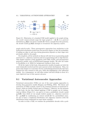
![9.1. VARIATIONAL AUTOENCODER APPROACHES 109
Figure 9.1: Illustration of a standard VAE model applied to the graph setting.
An encoder neural network maps the input graph G = (A, X) to a posterior
distribution qφ(Z|G) over latent variables Z. Given a sample from this posterior,
the decoder model pθ(A|Z) attempts to reconstruct the adjacency matrix.
graph node-by-node). These autoregressive approaches bear similarities to the
preferential attachment model from the previous chapter in that the probability
of adding an edge at each step during generation depends on what edges were
previously added to the graph.
For simplicity, all the methods we discuss will only focus on generating graph
structures (i.e., adjacency matrices) and not on generating node or edge features.
This chapter assumes a basic familiarity with VAEs, GANs, and autoregressive
generative models, such as LSTM-based language models. We refer the reader
to Goodfellow et al. [2016] for background reading in these areas.
Of all the topics in this book, deep generative models of graphs are both the
most technically involved and the most nascent in their development. Thus, our
goal in this chapter is to introduce the key methodological frameworks that have
inspired the early research in this area, while also highlighting a few influential
models. As a consequence, we will often eschew low-level details in favor of a
more high-level tour of this nascent sub-area.
9.1 Variational Autoencoder Approaches
Variational autoencoders (VAEs) are one of the most popular approaches to
develop deep generative models [Kingma and Welling, 2013]. The theory and
motivation of VAEs is deeply rooted in the statistical domain of variational in-
ference, which we briefly touched upon in Chapter 7. However, for the purposes
of this book, the key idea behind applying a VAE to graphs can be summa-
rized as follows (Figure 9.1): our goal is to train a probabilistic decoder model
pθ(A|Z), from which we can sample realistic graphs (i.e., adjacency matrices)
 ∼ pθ(A|Z) by conditioning on a latent variable Z. In a probabilistic sense,
we aim to learn a conditional distribution over adjacency matrices (with the
distribution being conditioned on some latent variable).
In order to train a VAE, we combine the probabilistic decoder with a prob-](https://image.slidesharecdn.com/grlbook-210914153141/85/Grl-book-118-320.jpg)
![110 CHAPTER 9. DEEP GENERATIVE MODELS
abilistic encoder model qθ(Z|G). This encoder model maps an input graph G to
a posterior distribution over the latent variable Z. The idea is that we jointly
train the encoder and decoder so that the decoder is able to reconstruct training
graphs given a latent variable Z ∼ qθ(Z|G) sampled from the encoder. Then,
after training, we can discard the encoder and generate new graphs by sam-
pling latent variables Z ∼ p(Z) from some (unconditional) prior distribution
and feeding these sampled latents to the decoder.
In more formal and mathematical detail, to build a VAE for graphs we must
specify the following key components:
1. A probabilistic encoder model qφ. In the case of graphs, the probabilistic
encoder model takes a graph G as input. From this input, qφ then defines
a distribution qφ(Z|G) over latent representations. Generally, in VAEs the
reparameterization trick with Gaussian random variables is used to design
a probabilistic qφ function. That is, we specify the latent conditional dis-
tribution as Z ∼ N(µφ(G), σ(φ(G)), where µφ and σφ are neural networks
that generate the mean and variance parameters for a normal distribution,
from which we sample latent embeddings Z.
2. A probabilistic decoder model pθ. The decoder takes a latent representation
Z as input and uses this input to specify a conditional distribution over
graphs. In this chapter, we will assume that pθ defines a conditional
distribution over the entries of the adjacency matrix, i.e., we can compute
pθ(A[u, v] = 1|Z).
3. A prior distribution p(Z) over the latent space. In this chapter we will
adopt the standard Gaussian prior Z ∼ N(0, 1), which is commonly used
for VAEs.
Given these components and a set of training graphs {G1, .., Gn}, we can
train a VAE model by minimizing the evidence likelihood lower bound (ELBO):
L =
X
Gi∈{G1,...,Gn}
Eqθ(Z|Gi)[pθ(Gi|Z)] − KL(qθ(Z|Gi)kp(Z)). (9.1)
The basic idea is that we seek to maximize the reconstruction ability of our
decoder—i.e., the likelihood term Eqθ(Z|Gi)[pθ(Gi|Z)]—while minimizing the KL-
divergence between our posterior latent distribution qθ(Z|Gi) and the prior p(Z).
The motivation behind the ELBO loss function is rooted in the theory of
variational inference [Wainwright and Jordan, 2008]. However, the key intuition
is that we want to generate a distribution over latent representations so that
the following two (conflicting) goals are satisfied:
1. The sampled latent representations encode enough information to allow
our decoder to reconstruct the input.
2. The latent distribution is as close as possible to the prior.](https://image.slidesharecdn.com/grlbook-210914153141/85/Grl-book-119-320.jpg)
![9.1. VARIATIONAL AUTOENCODER APPROACHES 111
The first goal ensures that we learn to decode meaningful graphs from the
encoded latent representations, when we have training graphs as input. The
second goal acts as a regularizer and ensures that we can decode meaningful
graphs even when we sample latent representations from the prior p(Z). This
second goal is critically important if we want to generate new graphs after
training: we can generate new graphs by sampling from the prior and feeding
these latent embeddings to the decoder, and this process will only work if this
second goal is satisfied.
In the following sections, we will describe two different ways in which the
VAE idea can be instantiated for graphs. The approaches differ in how they
define the encoder, decoder, and the latent representations. However, they share
the overall idea of adapting the VAE model to graphs.
9.1.1 Node-level Latents
The first approach we will examine builds closely upon the idea of encoding and
decoding graphs based on node embeddings, which we introduced in Chapter
3. The key idea in this approach is that that the encoder generates latent
representations for each node in the graph. The decoder then takes pairs of
embeddings as input and uses these embeddings to predict the likelihood of an
edge occurring between the two nodes. This idea was first proposed by Kipf
and Welling [2016b] and termed the Variational Graph Autoencoder (VGAE).
Encoder model
The encoder model in this setup can be based on any of the GNN architectures
we discussed in Chapter 5. In particular, given an adjacency matrix A and node
features X as input, we use two separate GNNs to generate mean and variance
parameters, respectively, conditioned on this input:
µZ = GNNµ(A, X) log σZ = GNNσ(A, X). (9.2)
Here, µZ is a |V| × d-dimensional matrix, which specifies a mean embedding
value for each node in the input graph. The log σZ ∈ R|V |×d
matrix similarly
specifies the log-variance for the latent embedding of each node.1
Given the encoded µZ and log σZ parameters, we can sample a set of latent
node embeddings by computing
Z = ◦ exp (log(σZ)) + µZ, (9.3)
where ∼ N(0, 1) is a |V| × d dimensional matrix with independently sampled
unit normal entries.
1Parameterizing the log-variance is often more stable than directly parameterizing the
variance.](https://image.slidesharecdn.com/grlbook-210914153141/85/Grl-book-120-320.jpg)
![112 CHAPTER 9. DEEP GENERATIVE MODELS
The decoder model
Given a matrix of sampled node embeddings Z ∈ R|V |×d
, the goal of the decoder
model is to predict the likelihood of all the edges in the graph. Formally, the
decoder must specify pθ(A|Z)—the posterior probability of the adjacency ma-
trix given the node embeddings. Again, here, many of the techniques we have
already discussed in this book can be employed, such as the various edge de-
coders introduced in Chapter 3. In the original VGAE paper, Kipf and Welling
[2016b] employ a simple dot-product decoder defined as follows:
pθ(A[u, v] = 1|zu, zv) = σ(z
u zv), (9.4)
where σ is used to denote the sigmoid function. Note, however, that a variety
of edge decoders could feasibly be employed, as long as these decoders generate
valid probability values.
To compute the reconstruction loss in Equation (9.1) using this approach,
we simply assume independence between edges and define the posterior pθ(G|Z)
over the full graph as follows:
pθ(G|Z) =
Y
(u,v)∈V2
pθ(A[u, v] = 1|zu, zv), (9.5)
which corresponds to a binary cross-entropy loss over the edge probabilities.
To generate discrete graphs after training, we can sample edges based on the
posterior Bernoulli distributions in Equation (9.4).
Limitations
The basic VGAE model sketched in the previous sections defines a valid gen-
erative model for graphs. After training this model to reconstruct a set of
training graphs, we could sample node embeddings Z from a standard normal
distribution and use our decoder to generate a graph. However, the generative
capacity of this basic approach is extremely limited, especially when a simple
dot-product decoder is used. The main issue is that the decoder has no param-
eters, so the model is not able to generate non-trivial graph structures without
a training graph as input. Indeed, in their initial work on the subject, Kipf and
Welling [2016b] proposed the VGAE model as an approach to generate node
embeddings, but they did not intend it as a generative model to sample new
graphs.
Some papers have proposed to address the limitations of VGAE as a gener-
ative model by making the decoder more powerful. For example, Grover et al.
[2019] propose to augment the decoder with an “iterative” GNN-based decoder.
Nonetheless, the simple node-level VAE approach has not emerged as a suc-
cessful and useful approach for graph generation. It has achieved strong results
on reconstruction tasks and as an autoencoder framework, but as a generative
model, this simple approach is severely limited.](https://image.slidesharecdn.com/grlbook-210914153141/85/Grl-book-121-320.jpg)
![9.1. VARIATIONAL AUTOENCODER APPROACHES 113
9.1.2 Graph-level Latents
As an alternative to the node-level VGAE approach described in the previous
section, one can also define variational autoencoders based on graph-level latent
representations. In this approach, we again use the ELBO loss (Equation 9.1) to
train a VAE model. However, we modify the encoder and decoder functions to
work with graph-level latent representations zG. The graph-level VAE described
in this section was first proposed by Simonovsky and Komodakis [2018], under
the name GraphVAE.
Encoder model
The encoder model in a graph-level VAE approach can be an arbitrary GNN
model augmented with a pooling layer. In particular, we will let GNN : Z|V|×|V|
×
R|V |×m
→ R||V |×d
denote any k-layer GNN, which outputs a matrix of node
embeddings, and we will use POOL : R||V |×d
→ Rd
to denote a pooling function
that maps a matrix of node embeddings Z ∈ R|V |×d
to a graph-level embedding
vector zG ∈ Rd
(as described in Chapter 5). Using this notation, we can define
the encoder for a graph-level VAE by the following equations:
µzG
= POOLµ (GNNµ(A, X)) log σzG
= POOLσ (GNNσ(A, X)) , (9.6)
where again we use two separate GNNs to parameterize the mean and variance of
a posterior normal distribution over latent variables. Note the critical difference
between this graph-level encoder and the node-level encoder from the previous
section: here, we are generating a mean µzG
∈ Rd
and variance parameter
log σzG
∈ Rd
for a single graph-level embedding zG ∼ N(µzG
, σzG
), whereas in
the previous section we defined posterior distributions for each individual node.
Decoder model
The goal of the decoder model in a graph-level VAE is to define pθ(G|zG),
the posterior distribution of a particular graph structure given the graph-level
latent embedding. The original GraphVAE model proposed to address this
challenge by combining a basic multi-layer perceptron (MLP) with a Bernoulli
distributional assumption [Simonovsky and Komodakis, 2018]. In this approach,
we use an MLP to map the latent vector zG to a matrix à ∈ [0, 1]|V|×|V|
of edge
probabilities:
à = σ (MLP(zG)) , (9.7)
where the sigmoid function σ is used to guarantee entries in [0, 1]. In principle,
we can then define the posterior distribution in an analogous way as the node-
level case:
pθ(G|zG) =
Y
(u,v)∈V
Ã[u, v]A[u, v] + (1 − Ã[u, v])(1 − A[u, v]), (9.8)
where A denotes the true adjacency matrix of graph G and à is our predicted
matrix of edge probabilities. In other words, we simply assume independent](https://image.slidesharecdn.com/grlbook-210914153141/85/Grl-book-122-320.jpg)
![114 CHAPTER 9. DEEP GENERATIVE MODELS
Bernoulli distributions for each edge, and the overall log-likelihood objective
is equivalent to set of independent binary cross-entropy loss function on each
edge. However, there are two key challenges in implementing Equation (9.8) in
practice:
1. First, if we are using an MLP as a decoder, then we need to assume
a fixed number of nodes. Generally, this problem is addressed by
assuming a maximum number of nodes and using a masking approach. In
particular, we can assume a maximum number of nodes nmax, which limits
the output dimension of the decoder MLP to matrices of size nmax ×nmax.
To decode a graph with |V| nmax nodes during training, we simply mask
(i.e., ignore) all entries in à with row or column indices greater than |V|.
To generate graphs of varying sizes after the model is trained, we can
specify a distribution p(n) over graph sizes with support {2, ..., nmax} and
sample from this distribution to determine the size of the generated graphs.
A simple strategy to specify p(n) is to use the empirical distribution of
graph sizes in the training data.
2. The second key challenge in applying Equation (9.8) in practice is that we
do not know the correct ordering of the rows and columns in Ã
when we are computing the reconstruction loss. The matrix à is
simply generated by an MLP, and when we want to use à to compute the
likelihood of a training graph, we need to implicitly assume some ordering
over the nodes (i.e., the rows and columns of Ã). Formally, the loss in
Equation (9.8) requires that we specify a node ordering π ∈ Π to order
the rows and columns in Ã.
This is important because if we simply ignore this issue, then the decoder
can overfit to the arbitrary node orderings used during training. There are
two popular strategies to address this issue. The first approach—proposed
by Simonovsky and Komodakis [2018]—is to apply a graph matching
heuristic to try to find the node ordering of à for each training graph
that gives the highest likelihood, which modifies the loss to
pθ(G|zG) = max
π∈Π
Y
(u,v)∈V
Ãπ
[u, v]A[u, v]+(1−Ãπ
[u, v])(1−A[u, v]), (9.9)
where we use Ãπ
to denote the predicted adjacency matrix under a specific
node ordering π. Unfortunately, however, computing the maximum in
Equation (9.9)—even using heuristic approximations—is computationally
expensive, and models based on graph matching are unable to scale to
graphs with more than hundreds of nodes. More recently, authors have
tended to use heuristic node orderings. For example, we can order nodes
based on a depth-first or breadth-first search starting from the highest-
degree node. In this approach, we simply specify a particular ordering
function π and compute the loss with this ordering:
pθ(G|zG) ≈
Y
(u,v)∈V
Ãπ
[u, v]A[u, v] + (1 − Ãπ
[u, v])(1 − A[u, v]),](https://image.slidesharecdn.com/grlbook-210914153141/85/Grl-book-123-320.jpg)
![9.2. ADVERSARIAL APPROACHES 115
or we consider a small set of heuristic orderings π1, ..., πn and average over
these orderings:
pθ(G|zG) ≈
X
πi∈{π1,...,πn}
Y
(u,v)∈V
Ãπi
[u, v]A[u, v]+(1−Ãπi
[u, v])(1−A[u, v]).
These heuristic orderings do not solve the graph matching problem, but
they seem to work well in practice. Liao et al. [2019a] provides a detailed
discussion and comparison of these heuristic ordering approaches, as well
as an interpretation of this strategy as a variational approximation.
Limitations
As with the node-level VAE approach, the basic graph-level framework has se-
rious limitations. Most prominently, using graph-level latent representations
introduces the issue of specifying node orderings, as discussed above. This
issue—together with the use of MLP decoders—currently limits the application
of the basic graph-level VAE to small graphs with hundreds of nodes or less.
However, the graph-level VAE framework can be combined with more effective
decoders—including some of the autoregressive methods we discuss in Section
9.3—which can lead to stronger models. We will mention one prominent exam-
ple of such as approach in Section 9.5, when we highlight the specific task of
generating molecule graph structures.
9.2 Adversarial Approaches
Variational autoencoders (VAEs) are a popular framework for deep generative
models—not just for graphs, but for images, text, and a wide-variety of data
domains. VAEs have a well-defined probabilistic motivation, and there are many
works that leverage and analyze the structure of the latent spaces learned by
VAE models. However, VAEs are also known to suffer from serious limitations—
such as the tendency for VAEs to produce blurry outputs in the image domain.
Many recent state-of-the-art generative models leverage alternative generative
frameworks, with generative adversarial networks (GANs) being one of the most
popular [Goodfellow et al., 2014].
The basic idea behind a general GAN-based generative models is as follows.
First, we define a trainable generator network gθ : Rd
→ X. This generator
network is trained to generate realistic (but fake) data samples x̃ ∈ X by taking
a random seed z ∈ Rd
as input (e.g., a sample from a normal distribution).
At the same time, we define a discriminator network dφ : X → [0, 1]. The
goal of the discriminator is to distinguish between real data samples x ∈ X
and samples generated by the generator x̃ ∈ X. Here, we will assume that
discriminator outputs the probability that a given input is fake.
To train a GAN, both the generator and discriminator are optimized jointly
in an adversarial game:
min
θ
max
φ
Ex∼pdata(x)[log(1 − dφ(x))] + Ez∼pseed(z)[log(dφ(gθ(z))], (9.10)](https://image.slidesharecdn.com/grlbook-210914153141/85/Grl-book-124-320.jpg)
![116 CHAPTER 9. DEEP GENERATIVE MODELS
where pdata(x) denotes the empirical distribution of real data samples (e.g.,
a uniform sample over a training set) and pseed(z) denotes the random seed
distribution (e.g., a standard multivariate normal distribution). Equation (9.10)
represents a minimax optimization problem. The generator is attempting to
minimize the discriminatory power of the discriminator, while the discriminator
is attempting to maximize its ability to detect fake samples. The optimization of
the GAN minimax objective—as well as more recent variations—is challenging,
but there is a wealth of literature emerging on this subject [Brock et al., 2018,
Heusel et al., 2017, Mescheder et al., 2018].
A basic GAN approach to graph generation
In the context of graph generation, a GAN-based approach was first employed
in concurrent work by Bojchevski et al. [2018] and De Cao and Kipf [2018]. The
basic approach proposed by De Cao and Kipf [2018]—which we focus on here—is
similar to the graph-level VAE discussed in the previous section. For instance,
for the generator, we can employ a simple multi-layer perceptron (MLP) to
generate a matrix of edge probabilities given a seed vector z:
à = σ (MLP(z)) , (9.11)
Given this matrix of edge probabilities, we can then generate a discrete adja-
cency matrix  ∈ Z|V|×|V|
by sampling independent Bernoulli variables for each
edge, with probabilities given by the entries of Ã; i.e., Â[u, v] ∼ Bernoulli(Ã[u, v]).
For the discriminator, we can employ any GNN-based graph classification model.
The generator model and the discriminator model can then be trained according
to Equation (9.10) using standard tools for GAN optimization.
Benefits and limitations of the GAN approach
As with the VAE approaches, the GAN framework for graph generation can be
extended in various ways. More powerful generator models can be employed—
for instance, leveraging the autoregressive techniques discussed in the next
section—and one can even incorporate node features into the generator and
discriminator models [De Cao and Kipf, 2018].
One important benefit of the GAN-based framework is that it removes the
complication of specifying a node ordering in the loss computation. As long as
the discriminator model is permutation invariant—which is the case for almost
every GNN—then the GAN approach does not require any node ordering to
be specified. The ordering of the adjacency matrix generated by the generator
is immaterial if the discriminator is permutation invariant. However, despite
this important benefit, GAN-based approaches to graph generation have so far
received less attention and success than their variational counterparts. This is
likely due to the difficulties involved in the minimax optimization that GAN-
based approaches require, and investigating the limits of GAN-based graph gen-
eration is currently an open problem.](https://image.slidesharecdn.com/grlbook-210914153141/85/Grl-book-125-320.jpg)
![9.3. AUTOREGRESSIVE METHODS 117
9.3 Autoregressive Methods
The previous two sections detailed how the ideas of variational autoencoding
(VAEs) and generative adversarial networks (GANs) can be applied to graph
generation. However, both the basic GAN and VAE-based approaches that we
discussed used simple multi-layer perceptrons (MLPs) to generate adjacency
matrices. In this section, we will introduce more sophisticated autoregressive
methods that can decode graph structures from latent representations. The
methods that we introduce in this section can be combined with the GAN and
VAE frameworks that we introduced previously, but they can also be trained as
standalone generative models.
9.3.1 Modeling Edge Dependencies
The simple generative models discussed in the previous sections assumed that
edges were generated independently. From a probabilistic perspective, we de-
fined the likelihood of a graph given a latent representation z by decomposing
the overall likelihood into a set of independent edge likelihoods as follows:
P(G|z) =
Y
(u,v)∈V2
P(A[u, v]|z). (9.12)
Assuming independence between edges is convenient, as it simplifies the likeli-
hood model and allows for efficient computations. However, it is a strong and
limiting assumption, since real-world graphs exhibit many complex dependen-
cies between edges. For example, the tendency for real-world graphs to have high
clustering coefficients is difficult to capture in an edge-independent model. To
alleviate this issue—while still maintaining tractability—autoregressive model
relax the assumption of edge independence.
Instead, in the autoregressive approach, we assume that edges are generated
sequentially and that the likelihood of each edge can be conditioned on the edges
that have been previously generated. To make this idea precise, we will use L
to denote the lower-triangular portion of the adjacency matrix A. Assuming we
are working with simple graphs, A and L contain exactly the same information,
but it will be convenient to work with L in the following equations. We will then
use the notation L[v1, :] to denote the row of L corresponding to node v1, and we
will assume that the rows of L are indexed by nodes v1, ..., v|V|. Note that due to
the lower-triangular nature of L, we will have that L[vi, vj] = 0, ∀j i, meaning
that we only need to be concerned with generating the first i entries for any
row L[vi, :]; the rest can simply be padded with zeros. Given this notation, the
autoregressive approach amounts to the following decomposition of the overall
graph likelihood:
P(G|z) =
|V|
Y
i=1
P(L[vi, :]|L[v1, :], ..., L[vi−1, :], z). (9.13)
In other words, when we generate row L[vi, :], we condition on all the previous
generated rows L[vj, :] with j i.](https://image.slidesharecdn.com/grlbook-210914153141/85/Grl-book-126-320.jpg)
![118 CHAPTER 9. DEEP GENERATIVE MODELS
9.3.2 Recurrent Models for Graph Generation
We will now discuss two concrete instantiations of the autoregressive generation
idea. These two approaches build upon ideas first proposed in Li et al. [2018]
and are generally indicative of the strategies that one could employ for this
task. In the first model we will review—called GraphRNN [You et al., 2018]—we
model autoregressive dependencies using a recurrent neural network (RNN). In
the second approach—called graph recurrent attention network (GRAN) [Liao
et al., 2019a]—we generate graphs by using a GNN to condition on the adjacency
matrix that has been generated so far.
GraphRNN
The first model to employ this autoregressive generation approach was GraphRNN
[You et al., 2018]. The basic idea in the GraphRNN approach is to use a hier-
archical RNN to model the edge dependencies in Equation (9.13).
The first RNN in the hierarchical model—termed the graph-level RNN—is
used to model the state of the graph that has been generated so far. Formally,
the graph-level RNN maintains a hidden state hi, which is updated after gen-
erating each row of the adjacency matrix L[vi, :]:
hi+1 = RNNgraph(hi, L[vi, L]), (9.14)
where we use RNNgraph to denote a generic RNN state update with hi cor-
responding to the hidden state and L[vi, L] to the observation.2
In You et al.
[2018]’s original formulation, a fixed initial hidden state h0 = 0 is used to initial-
ize the graph-level RNN, but in principle this initial hidden state could also be
learned by a graph encoder model or sampled from a latent space in a VAE-style
approach.
The second RNN—termed the node-level RNN or RNNnode—generates the
entries of L[vi, :] in an autoregressive manner. RNNnode takes the graph-level
hidden state hi as an initial input and then sequentially generates the binary
values of L[vi, ; ], assuming a conditional Bernoulli distribution for each entry.
The overall GraphRNN approach is called hierarchical because the node-level
RNN is initialized at each time-step with the current hidden state of the graph-
level RNN.
Both the graph-level RNNgraph and the node-level RNNnode can be opti-
mized to maximize the likelihood the training graphs (Equation 9.13) using the
teaching forcing strategy [Williams and Zipser, 1989], meaning that the ground
truth values of L are always used to update the RNNs during training. To
control the size of the generated graphs, the RNNs are also trained to output
end-of-sequence tokens, which are used to specify the end of the generation pro-
cess. Note that—as with the graph-level VAE approaches discussed in Section
9.1—computing the likelihood in Equation (9.13) requires that we assume a
particular ordering over the generated nodes.
2You et al. [2018] use GRU-style RNNs but in principle LSTMs or other RNN architecture
could be employed.](https://image.slidesharecdn.com/grlbook-210914153141/85/Grl-book-127-320.jpg)
![9.3. AUTOREGRESSIVE METHODS 119
Figure 9.2: Illustration of the GRAN generation approach [Liao et al., 2019a].
After training to maximize the likelihood of the training graphs (Equation
9.13), the GraphRNN model can be used to generate graphs at test time by
simply running the hierarchical RNN starting from the fixed, initial hidden
state h0. Since the edge-level RNN involves a stochastic sampling process to
generate the discrete edges, the GraphRNN model is able to generate diverse
samples of graphs even when a fixed initial embedding is used. However—
as mentioned above—the GraphRNN model could, in principle, be used as a
decoder or generator within a VAE or GAN framework, respectively.
Graph Recurrent Attention Networks (GRAN)
The key benefit of the GraphRNN approach—discussed above—is that it mod-
els dependencies between edges. Using an autoregressive modeling assumption
(Equation 9.13), GraphRNN can condition the generation of edges at generation
step i based on the state of the graph that has already been generated during
generation steps 1, ...i − 1. Conditioning in this way makes it much easier to
generate complex motifs and regular graph structures, such as grids. For ex-
ample, in Figure 9.3, we can see that GraphRNN is more capable of generating
grid-like structures, compared to the basic graph-level VAE (Section 9.1). How-
ever, the GraphRNN approach still has serious limitations. As we can see in
Figure 9.3, the GraphRNN model still generates unrealistic artifacts (e.g., long
chains) when trained on samples of grids. Moreover, GraphRNN can be difficult
to train and scale to large graphs due to the need to backpropagate through
many steps of RNN recurrence.
To address some of the limitations of the GraphRNN approach, Liao et al.
[2019a] proposed the GRAN model. GRAN—which stands for graph recurrent
attention networks—maintains the autoregressive decomposition of the gener-
ation process. However, instead of using RNNs to model the autoregressive
generation process, GRAN uses GNNs. The key idea in GRAN is that we
can model the conditional distribution of each row of the adjacency matrix by
running a GNN on the graph that has been generated so far (Figure 9.2):
P(L[vi, :]|L[v1, :], ..., L[vi−1, :], z) ≈ GNN(L[v1 : vi−1, :], X̃). (9.15)](https://image.slidesharecdn.com/grlbook-210914153141/85/Grl-book-128-320.jpg)
![120 CHAPTER 9. DEEP GENERATIVE MODELS
Here, we use L[v1 : vi−1, :] to denote the lower-triangular adjacency matrix of the
graph that has been generated up to generation step i. The GNN in Equation
(9.15) can be instantiated in many ways, but the crucial requirement is that
it generates a vector of edge probabilities L[vi, :], from which we can sample
discrete edge realizations during generation. For example, Liao et al. [2019a]
use a variation of the graph attention network (GAT) model (see Chapter 5) to
define this GNN. Finally, since there are no node attributes associated with the
generated nodes, the input feature matrix X̃ to the GNN can simply contain
randomly sampled vectors (which are useful to distinguish between nodes).
The GRAN model can be trained in an analogous manner as GraphRNN
by maximizing the likelihood of training graphs (Equation 9.13) using teacher
forcing. Like the GraphRNN model, we must also specify an ordering over nodes
to compute the likelihood on training graphs, and Liao et al. [2019a] provides a
detailed discussion on this challenge. Lastly, like the GraphRNN model, we can
use GRAN as a generative model after training simply by running the stochastic
generation process (e.g., from a fixed initial state), but this model could also be
integrated into VAE or GAN-based frameworks.
The key benefit of the GRAN model—compared to GraphRNN—is that it
does not need to maintain a long and complex history in a graph-level RNN.
Instead, the GRAN model explicitly conditions on the already generated graph
using a GNN at each generation step. Liao et al. [2019a] also provide a de-
tailed discussion on how the GRAN model can be optimized to facilitate the
generation of large graphs with hundreds of thousands of nodes. For example,
one key performance improvement is the idea that multiple nodes can be added
simultaneously in a single block, rather than adding nodes one at a time. This
idea is illustrated in Figure 9.2.
9.4 Evaluating Graph Generation
The previous three sections introduced a series of increasingly sophisticated
graph generation approaches, based on VAEs, GANs, and autoregressive mod-
els. As we introduced these approaches, we hinted at the superiority of some
approaches over others. We also provided some examples of generated graphs
in Figure 9.3, which hint at the varying capabilities of the different approaches.
However, how do we actually quantitatively compare these different models?
How can we say that one graph generation approach is better than another?
Evaluating generative models is a challenging task, as there is no natural notion
of accuracy or error. For example, we could compare reconstruction losses or
model likelihoods on held out graphs, but this is complicated by the lack of a
uniform likelihood definition across different generation approaches.
In the case of general graph generation, the current practice is to analyze
different statistics of the generated graphs, and to compare the distribution of
statistics for the generated graphs to a test set [Liao et al., 2019a]. Formally,
assume we have set of graph statistics S = (s1, s2, ..., sn), where each of these
statistics si,G : R → [0, 1] is assumed to define a univariate distribution over R](https://image.slidesharecdn.com/grlbook-210914153141/85/Grl-book-129-320.jpg)
![9.5. MOLECULE GENERATION 121
Figure 9.3: Examples of graphs generated by a basic graph-level VAE (Section
9.1), as well as the GraphRNN and GRAN models. Each row corresponds to
a different dataset. The first column shows an example of a real graph from
the dataset, while the other columns are randomly selected samples of graphs
generated by the corresponding model [Liao et al., 2019a].
for a given graph G. For example, for a given graph G, we can compute the degree
distribution, the distribution of clustering coefficients, and the distribution of
different motifs or graphlets. Given a particular statistic si—computed on both
a test graph si,Gtest and a generated graph si,Ggen —we can compute the distance
between the statistic’s distribution on the test graph and generated graph using
a distributional measure, such as the total variation distance:
d(si,Gtest
, si,Ggen
) = sup
x∈R
|si,Gtest
(x) − si,Ggen
(x)|. (9.16)
To get measure of performance, we can compute the average pairwise distribu-
tional distance between a set of generated graphs and graphs in a test set.
Existing works have used this strategy with graph statistics such as degree
distributions, graphlet counts, and spectral features, with distributional dis-
tances computed using variants of the total variation score and the first Wasser-
stein distance [Liao et al., 2019b, You et al., 2018].
9.5 Molecule Generation
All the graph generation approaches we introduced so far are useful for gen-
eral graph generation. The previous sections did not assume a particular data
domain, and our goal was simply to generate realistic graph structures (i.e.,](https://image.slidesharecdn.com/grlbook-210914153141/85/Grl-book-130-320.jpg)
![122 CHAPTER 9. DEEP GENERATIVE MODELS
adjacency matrices) based on a given training set of graphs. It is worth not-
ing, however, that many works within the general area of graph generation are
focused specifically on the task of molecule generation.
The goal of molecule generation is to generate molecular graph structures
that are both valid (e.g., chemically stable) and ideally have some desirable
properties (e.g., medicinal properties or solubility). Unlike the general graph
generation problem, research on molecule generation can benefit substantially
from domain-specific knowledge for both model design and evaluation strategies.
For example, Jin et al. [2018] propose an advanced variant of the graph-level
VAE approach (Section 9.1) that leverages knowledge about known molecular
motifs. Given the strong dependence on domain-specific knowledge and the
unique challenges of molecule generation compared to general graphs, we will
not review these approaches in detail here. Nonetheless, it is important to
highlight this domain as one of the fastest growing subareas of graph generation.](https://image.slidesharecdn.com/grlbook-210914153141/85/Grl-book-131-320.jpg)
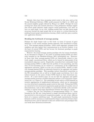
![124 Conclusion
Already, there have been promising initial works in this area, such as the
Neural Relational Inference (NRI) model proposed by Kipf et al. [2018] and
the nearest-neighbor graphs inferred by Wang et al. [2019]. Perhaps the most
exciting fact about this research direction is that preliminary findings suggest
that latent graph inference might improve model performance even when we
have an input graph. In my view, building models that can infer latent graph
structures beyond the input graph that we are given is a critical direction for
pushing forward graph representation learning, which could also open countless
new application domains.
Breaking the bottleneck of message passing
Perhaps the single largest topic in this book—in terms of amount of space
dedicated—is the neural message passing approach, first introduced in Chap-
ter 5. This message passing formalism—where nodes aggregate messages from
neighbors and then update their representations in an iterative fashion—is at
the heart of current GNNs and has become the dominant paradigm in graph
representation learning.
However, the neural message passing paradigm also has serious drawbacks.
As we discussed in Chapter 7, the power of message-passing GNNs are inher-
ently bounded by the Weisfeiler-Lehman (WL) isomorphism test. Moreover,
we know that these message-passing GNNs are theoretically related to rela-
tively simple convolutional filters, which can be formed by polynomials of the
(normalized) adjacency matrix. Empirically, researchers have continually found
message-passing GNNs to suffer from the problem of over-smoothing, and this
issue of over-smoothing can be viewed as a consequence of the neighborhood
aggregation operation, which is at the core of current GNNs. Indeed, at their
core message-passing GNNs are inherently limited by the aggregate and update
message-passing paradigm. This paradigm induces theoretical connections to
the WL isomorphism test as well as to simple graph convolutions, but it also
induces bounds on the power of these GNNs based on these theoretical con-
structs. At a more intuitive level, we can see that the aggregate and update
message-passing structure of GNNs inherently induces a tree-structured compu-
tation (see, e.g., Figure 5.1). The embedding of each node in a GNN depends on
iterative aggregations of neighborhood information, which can be represented
as a tree-structured computation graph rooted at that node. Noting that GNNs
are restricted to tree-structured computation graph provides yet another view of
their limitations, such as their inability to consistently identify cycles and their
inability to capture long-range dependencies between the nodes in a graph.
I believe that the core limitations of message-passing GNNs—i.e., being
bounded by the WL test, being limited to simple convolutional filters, and be-
ing restricted to tree-structured computation graphs—are all, in fact, different
facets of a common underlying cause. To push graph representation learning
forward, it will be necessary to understand the deeper connections between these
theoretical views, and we will need to find new architectures and paradigms that
can break these theoretical bottlenecks.](https://image.slidesharecdn.com/grlbook-210914153141/85/Grl-book-133-320.jpg)