MatConvNet is a MATLAB toolbox that implements convolutional neural networks for computer vision tasks. It provides functions for common CNN layers like convolution, pooling, and normalization. These can be combined to easily prototype new CNN architectures. MatConvNet supports efficient GPU computation, allowing it to train complex models on large datasets. It aims to be a simple and flexible environment for computer vision researchers to experiment with CNNs within the MATLAB platform.


![Chapter 1
Introduction to MatConvNet
MatConvNet is a MATLAB toolbox implementing Convolutional Neural Networks (CNN)
for computer vision applications. Since the breakthrough work of [8], CNNs have had a
major impact in computer vision, and image understanding in particular, essentially replacing
traditional image representations such as the ones implemented in our own VLFeat [13] open
source library.
While most CNNs are obtained by composing simple linear and non-linear filtering op-
erations such as convolution and rectification, their implementation is far from trivial. The
reason is that CNNs need to be learned from vast amounts of data, often millions of images,
requiring very efficient implementations. As most CNN libraries, MatConvNet achieves
this by using a variety of optimizations and, chiefly, by supporting computations on GPUs.
Numerous other machine learning, deep learning, and CNN open source libraries exist.
To cite some of the most popular ones: CudaConvNet,1
Torch,2
Theano,3
and Caffe4
. Many
of these libraries are well supported, with dozens of active contributors and large user bases.
Therefore, why creating yet another library?
The key motivation for developing MatConvNet was to provide an environment par-
ticularly friendly and efficient for researchers to use in their investigations.5
MatConvNet
achieves this by its deep integration in the MATLAB environment, which is one of the most
popular development environments in computer vision research as well as in many other areas.
In particular, MatConvNet exposes as simple MATLAB commands CNN building blocks
such as convolution, normalisation and pooling (chapter 4); these can then be combined and
extended with ease to create CNN architectures. While many of such blocks use optimised
CPU and GPU implementations written in C++ and CUDA (section section 1.4), MATLAB
native support for GPU computation means that it is often possible to write new blocks
in MATLAB directly while maintaining computational efficiency. Compared to writing new
CNN components using lower level languages, this is an important simplification that can
significantly accelerate testing new ideas. Using MATLAB also provides a bridge towards
1
https://code.google.com/p/cuda-convnet/
2
http://cilvr.nyu.edu/doku.php?id=code:start
3
http://deeplearning.net/software/theano/
4
http://caffe.berkeleyvision.org
5
While from a user perspective MatConvNet currently relies on MATLAB, the library is being devel-
oped with a clean separation between MATLAB code and the C++ and CUDA core; therefore, in the future
the library may be extended to allow processing convolutional networks independently of MATLAB.
1](https://image.slidesharecdn.com/matconvnet-manual-231016102442-4505fd2a/85/matconvnet-manual-pdf-5-320.jpg)
![2 CHAPTER 1. INTRODUCTION TO MATCONVNET
other areas; for instance, MatConvNet was recently used by the University of Arizona in
planetary science, as summarised in this NVIDIA blogpost.6
MatConvNet can learn large CNN models such AlexNet [8] and the very deep networks
of [11] from millions of images. Pre-trained versions of several of these powerful models can
be downloaded from the MatConvNet home page7
. While powerful, MatConvNet re-
mains simple to use and install. The implementation is fully self-contained, requiring only
MATLAB and a compatible C++ compiler (using the GPU code requires the freely-available
CUDA DevKit and a suitable NVIDIA GPU). As demonstrated in fig. 1.1 and section 1.1,
it is possible to download, compile, and install MatConvNet using three MATLAB com-
mands. Several fully-functional examples demonstrating how small and large networks can
be learned are included. Importantly, several standard pre-trained network can be immedi-
ately downloaded and used in applications. A manual with a complete technical description
of the toolbox is maintained along with the toolbox.8
These features make MatConvNet
useful in an educational context too.9
MatConvNet is open-source released under a BSD-like license. It can be downloaded
from http://www.vlfeat.org/matconvnet as well as from GitHub.10
.
1.1 Getting started
MatConvNet is simple to install and use. fig. 1.1 provides a complete example that clas-
sifies an image using a latest-generation deep convolutional neural network. The example
includes downloading MatConvNet, compiling the package, downloading a pre-trained CNN
model, and evaluating the latter on one of MATLAB’s stock images.
The key command in this example is vl_simplenn, a wrapper that takes as input the
CNN net and the pre-processed image im_ and produces as output a structure res of results.
This particular wrapper can be used to model networks that have a simple structure, namely
a chain of operations. Examining the code of vl_simplenn (edit vl_simplenn in MatCon-
vNet) we note that the wrapper transforms the data sequentially, applying a number of
MATLAB functions as specified by the network configuration. These function, discussed in
detail in chapter 4, are called “building blocks” and constitute the backbone of MatCon-
vNet.
While most blocks implement simple operations, what makes them non trivial is their
efficiency (section 1.4) as well as support for backpropagation (section 2.3) to allow learning
CNNs. Next, we demonstrate how to use one of such building blocks directly. For the sake of
the example, consider convolving an image with a bank of linear filters. Start by reading an
image in MATLAB, say using im = single(imread('peppers.png')), obtaining a H × W × D
array im, where D = 3 is the number of colour channels in the image. Then create a bank
of K = 16 random filters of size 3 × 3 using f = randn(3,3,3,16,'single'). Finally, convolve the
6
http://devblogs.nvidia.com/parallelforall/deep-learning-image-understanding-planetary-scien
7
http://www.vlfeat.org/matconvnet/
8
http://www.vlfeat.org/matconvnet/matconvnet-manual.pdf
9
An example laboratory experience based on MatConvNet can be downloaded from http://www.
robots.ox.ac.uk/~vgg/practicals/cnn/index.html.
10
http://www.github.com/matconvnet](https://image.slidesharecdn.com/matconvnet-manual-231016102442-4505fd2a/85/matconvnet-manual-pdf-6-320.jpg)
![1.1. GETTING STARTED 3
% install and compile MatConvNet (run once)
untar(['http://www.vlfeat.org/matconvnet/download/' ...
'matconvnet−1.0−beta25.tar.gz']) ;
cd matconvnet−1.0−beta25
run matlab/vl_compilenn
% download a pre−trained CNN from the web (run once)
urlwrite(...
'http://www.vlfeat.org/matconvnet/models/imagenet−vgg−f.mat', ...
'imagenet−vgg−f.mat') ;
% setup MatConvNet
run matlab/vl_setupnn
% load the pre−trained CNN
net = load('imagenet−vgg−f.mat') ;
% load and preprocess an image
im = imread('peppers.png') ;
im_ = imresize(single(im), net.meta.normalization.imageSize(1:2)) ;
im_ = im_ − net.meta.normalization.averageImage ;
% run the CNN
res = vl_simplenn(net, im_) ;
% show the classification result
scores = squeeze(gather(res(end).x)) ;
[bestScore, best] = max(scores) ;
figure(1) ; clf ; imagesc(im) ;
bell pepper (946), score 0.704
title(sprintf('%s (%d), score %.3f',...
net.classes.description{best}, best, bestScore)) ;
Figure 1.1: A complete example including download, installing, compiling and running Mat-
ConvNet to classify one of MATLAB stock images using a large CNN pre-trained on
ImageNet.](https://image.slidesharecdn.com/matconvnet-manual-231016102442-4505fd2a/85/matconvnet-manual-pdf-7-320.jpg)
![4 CHAPTER 1. INTRODUCTION TO MATCONVNET
image with the filters by using the command y = vl_nnconv(x,f,[]). This results in an array
y with K channels, one for each of the K filters in the bank.
While users are encouraged to make use of the blocks directly to create new architectures,
MATLAB provides wrappers such as vl_simplenn for standard CNN architectures such as
AlexNet [8] or Network-in-Network [9]. Furthermore, the library provides numerous examples
(in the examples/ subdirectory), including code to learn a variety of models on the MNIST,
CIFAR, and ImageNet datasets. All these examples use the examples/cnn_train training
code, which is an implementation of stochastic gradient descent (section 3.3). While this
training code is perfectly serviceable and quite flexible, it remains in the examples/ subdirec-
tory as it is somewhat problem-specific. Users are welcome to implement their optimisers.
1.2 MatConvNet at a glance
MatConvNet has a simple design philosophy. Rather than wrapping CNNs around complex
layers of software, it exposes simple functions to compute CNN building blocks, such as linear
convolution and ReLU operators, directly as MATLAB commands. These building blocks are
easy to combine into complete CNNs and can be used to implement sophisticated learning
algorithms. While several real-world examples of small and large CNN architectures and
training routines are provided, it is always possible to go back to the basics and build your
own, using the efficiency of MATLAB in prototyping. Often no C coding is required at all
to try new architectures. As such, MatConvNet is an ideal playground for research in
computer vision and CNNs.
MatConvNet contains the following elements:
ˆ CNN computational blocks. A set of optimized routines computing fundamental
building blocks of a CNN. For example, a convolution block is implemented by
y=vl_nnconv(x,f,b) where x is an image, f a filter bank, and b a vector of biases (sec-
tion 4.1). The derivatives are computed as [dzdx,dzdf,dzdb] = vl_nnconv(x,f,b,dzdy)
where dzdy is the derivative of the CNN output w.r.t y (section 4.1). chapter 4 de-
scribes all the blocks in detail.
ˆ CNN wrappers. MatConvNet provides a simple wrapper, suitably invoked by
vl_simplenn, that implements a CNN with a linear topology (a chain of blocks). It also
provides a much more flexible wrapper supporting networks with arbitrary topologies,
encapsulated in the dagnn.DagNN MATLAB class.
ˆ Example applications. MatConvNet provides several examples of learning CNNs with
stochastic gradient descent and CPU or GPU, on MNIST, CIFAR10, and ImageNet
data.
ˆ Pre-trained models. MatConvNet provides several state-of-the-art pre-trained CNN
models that can be used off-the-shelf, either to classify images or to produce image
encodings in the spirit of Caffe or DeCAF.](https://image.slidesharecdn.com/matconvnet-manual-231016102442-4505fd2a/85/matconvnet-manual-pdf-8-320.jpg)
![1.3. DOCUMENTATION AND EXAMPLES 5
epoch
0 10 20 30 40 50 60
0.2
0.3
0.4
0.5
0.6
0.7
0.8
0.9
dropout top-1 val
dropout top-5 val
bnorm top-1 val
bnorm top-5 val
Figure 1.2: Training AlexNet on ImageNet ILSVRC: dropout vs batch normalisation.
1.3 Documentation and examples
There are three main sources of information about MatConvNet. First, the website con-
tains descriptions of all the functions and several examples and tutorials.11
Second, there
is a PDF manual containing a great deal of technical details about the toolbox, including
detailed mathematical descriptions of the building blocks. Third, MatConvNet ships with
several examples (section 1.1).
Most examples are fully self-contained. For example, in order to run the MNIST example,
it suffices to point MATLAB to the MatConvNet root directory and type addpath ←-
examples followed by cnn_mnist. Due to the problem size, the ImageNet ILSVRC example
requires some more preparation, including downloading and preprocessing the images (using
the bundled script utils/preprocess−imagenet.sh). Several advanced examples are included
as well. For example, fig. 1.2 illustrates the top-1 and top-5 validation errors as a model
similar to AlexNet [8] is trained using either standard dropout regularisation or the recent
batch normalisation technique of [4]. The latter is shown to converge in about one third of
the epochs (passes through the training data) required by the former.
The MatConvNet website contains also numerous pre-trained models, i.e. large CNNs
trained on ImageNet ILSVRC that can be downloaded and used as a starting point for many
other problems [1]. These include: AlexNet [8], VGG-S, VGG-M, VGG-S [1], and VGG-VD-
16, and VGG-VD-19 [12]. The example code of fig. 1.1 shows how one such model can be
used in a few lines of MATLAB code.
11
See also http://www.robots.ox.ac.uk/~vgg/practicals/cnn/index.html.](https://image.slidesharecdn.com/matconvnet-manual-231016102442-4505fd2a/85/matconvnet-manual-pdf-9-320.jpg)
![6 CHAPTER 1. INTRODUCTION TO MATCONVNET
model batch sz. CPU GPU CuDNN
AlexNet 256 22.1 192.4 264.1
VGG-F 256 21.4 211.4 289.7
VGG-M 128 7.8 116.5 136.6
VGG-S 128 7.4 96.2 110.1
VGG-VD-16 24 1.7 18.4 20.0
VGG-VD-19 24 1.5 15.7 16.5
Table 1.1: ImageNet training speed (images/s).
1.4 Speed
Efficiency is very important for working with CNNs. MatConvNet supports using NVIDIA
GPUs as it includes CUDA implementations of all algorithms (or relies on MATLAB CUDA
support).
To use the GPU (provided that suitable hardware is available and the toolbox has been
compiled with GPU support), one simply converts the arguments to gpuArrays in MATLAB,
as in y = vl_nnconv(gpuArray(x), gpuArray(w), []). In this manner, switching between CPU
and GPU is fully transparent. Note that MatConvNet can also make use of the NVIDIA
CuDNN library with significant speed and space benefits.
Next we evaluate the performance of MatConvNet when training large architectures
on the ImageNet ILSVRC 2012 challenge data [2]. The test machine is a Dell server with
two Intel Xeon CPU E5-2667 v2 clocked at 3.30 GHz (each CPU has eight cores), 256 GB
of RAM, and four NVIDIA Titan Black GPUs (only one of which is used unless otherwise
noted). Experiments use MatConvNet beta12, CuDNN v2, and MATLAB R2015a. The
data is preprocessed to avoid rescaling images on the fly in MATLAB and stored in a RAM
disk for faster access. The code uses the vl_imreadjpeg command to read large batches of
JPEG images from disk in a number of separate threads. The driver examples/cnn_imagenet.m
is used in all experiments.
We train the models discussed in section 1.3 on ImageNet ILSVRC. table 1.1 reports
the training speed as number of images per second processed by stochastic gradient descent.
AlexNet trains at about 264 images/s with CuDNN, which is about 40% faster than the
vanilla GPU implementation (using CuBLAS) and more than 10 times faster than using the
CPUs. Furthermore, we note that, despite MATLAB overhead, the implementation speed is
comparable to Caffe (they report 253 images/s with CuDNN and a Titan – a slightly slower
GPU than the Titan Black used here). Note also that, as the model grows in size, the size of
a SGD batch must be decreased (to fit in the GPU memory), increasing the overhead impact
somewhat.
table 1.2 reports the speed on VGG-VD-16, a very large model, using multiple GPUs. In
this case, the batch size is set to 264 images. These are further divided in sub-batches of 22
images each to fit in the GPU memory; the latter are then distributed among one to four
GPUs on the same machine. While there is a substantial communication overhead, training
speed increases from 20 images/s to 45. Addressing this overhead is one of the medium term
goals of the library.](https://image.slidesharecdn.com/matconvnet-manual-231016102442-4505fd2a/85/matconvnet-manual-pdf-10-320.jpg)
![1.5. ACKNOWLEDGMENTS 7
num GPUs 1 2 3 4
VGG-VD-16 speed 20.0 22.20 38.18 44.8
Table 1.2: Multiple GPU speed (images/s).
1.5 Acknowledgments
MatConvNet is a community project, and as such acknowledgements go to all contributors.
We kindly thank NVIDIA supporting this project by providing us with top-of-the-line GPUs
and MathWorks for ongoing discussion on how to improve the library.
The implementation of several CNN computations in this library are inspired by the Caffe
library [6] (however, Caffe is not a dependency). Several of the example networks have been
trained by Karen Simonyan as part of [1] and [12].](https://image.slidesharecdn.com/matconvnet-manual-231016102442-4505fd2a/85/matconvnet-manual-pdf-11-320.jpg)


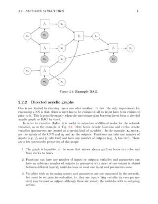
![12 CHAPTER 2. NEURAL NETWORK COMPUTATIONS
4. Since the graph is acyclic, the CNN can be evaluated by sorting the functions and
computing them one after another (in the example, evaluating the functions in the
order f1, f2, f3, f4, f5 would work).
2.3 Computing derivatives with backpropagation
Learning a NN requires computing the derivative of the loss with respect to the network
parameters. Derivatives are computed using an algorithm called backpropagation, which is
a memory-efficient implementation of the chain rule for derivatives. First, we discuss the
derivatives of a single layer, and then of a whole network.
2.3.1 Derivatives of tensor functions
In a CNN, a layer is a function y = f(x) where both input x ∈ RH×W×C
and output
y ∈ RH0×W0×C0
are tensors. The derivative of the function f contains the derivative of
each output component yi0j0k0 with respect to each input component xijk, for a total of
H0
×W0
×C0
×H ×W ×C elements naturally arranged in a 6D tensor. Instead of expressing
derivatives as tensors, it is often useful to switch to a matrix notation by stacking the input
and output tensors into vectors. This is done by the vec operator, which visits each element
of a tensor in lexicographical order and produces a vector:
vec x =
x111
x211
.
.
.
xH11
x121
.
.
.
xHWC
.
By stacking both input and output, each layer f can be seen reinterpreted as vector function
vec f, whose derivative is the conventional Jacobian matrix:
d vec f
d(vec x)>
=
∂y111
∂x111
∂y111
∂x211
. . . ∂y111
∂xH11
∂y111
∂x121
. . . ∂y111
∂xHW C
∂y211
∂x111
∂y211
∂x211
. . . ∂y211
∂xH11
∂y211
∂x121
. . . ∂y211
∂xHW C
.
.
.
.
.
. . . .
.
.
.
.
.
. . . .
.
.
.
∂yH011
∂x111
∂yH011
∂x211
. . .
∂yH011
∂xH11
∂yH011
∂x121
. . .
∂yH011
∂xHW C
∂y121
∂x111
∂y121
∂x211
. . . ∂y121
∂xH11
∂y121
∂x121
. . . ∂y121
∂xHW C
.
.
.
.
.
. . . .
.
.
.
.
.
. . . .
.
.
.
∂yH0W 0C0
∂x111
∂yH0W 0C0
∂x211
. . .
∂yH0W 0C0
∂xH11
∂yH0W 0C0
∂x121
. . .
∂yH0W 0C0
∂xHW C
.
This notation for the derivatives of tensor functions is taken from [7] and is used throughout
this document.](https://image.slidesharecdn.com/matconvnet-manual-231016102442-4505fd2a/85/matconvnet-manual-pdf-16-320.jpg)
![2.3. COMPUTING DERIVATIVES WITH BACKPROPAGATION 13
While it is easy to express the derivatives of tensor functions as matrices, these matrices
are in general extremely large. Even for moderate data sizes (e.g. H = H0
= W = W0
=
32 and C = C0
= 128), there are H0
W0
C0
HWC ≈ 17 × 109
elements in the Jacobian.
Storing that requires 68 GB of space in single precision. The purpose of the backpropagation
algorithm is to compute the derivatives required for learning without incurring this huge
memory cost.
2.3.2 Derivatives of function compositions
In order to understand backpropagation, consider first a simple CNN terminating in a loss
function fL = `y:
x0 f1 f2
... fL
w1 w2 wL
xl ∈ R
x1 x2 xL−1
The goal is to compute the gradient of the loss value xL (output) with respect to each network
parameter wl:
df
d(vec wl)>
=
d
d(vec wl)>
[fL(·; wL) ◦ ... ◦ f2(·; w2) ◦ f1(x0; w1)] .
By applying the chain rule and by using the matrix notation introduced above, the derivative
can be written as
df
d(vec wl)>
=
d vec fL(xL−1; wL)
d(vec xL−1)>
× · · · ×
d vec fl+1(xl; wl+1)
d(vec xl)>
×
d vec fl(xl−1; wl)
d(vec w>
l )
(2.1)
where the derivatives are computed at the working point determined by the input x0 and the
current value of the parameters.
Note that, since the network output xl is a scalar quantity, the target derivative
df/d(vec wl)>
has the same number of elements of the parameter vector wl, which is moder-
ate. However, the intermediate Jacobian factors have, as seen above, an unmanageable size.
In order to avoid computing these factor explicitly, we can proceed as follows.
Start by multiplying the output of the last layer by a tensor pL = 1 (note that this tensor
is a scalar just like the variable xL):
pL ×
df
d(vec wl)>
= pL ×
d vec fL(xL−1; wL)
d(vec xL−1)>
| {z }
(vec pL−1)>
× · · · ×
d vec fl+1(xl; wl+1)
d(vec xl)>
×
d vec fl(xl−1; wl)
d(vec w>
l )
= (vec pL−1)>
× · · · ×
d vec fl+1(xl; wl+1)
d(vec xl)>
×
d vec fl(xl−1; wl)
d(vec w>
l )
In the second line the last two factors to the left have been multiplied obtaining a new
tensor pL−1 that has the same size as the variable xL−1. The factor pL−1 can therefore be](https://image.slidesharecdn.com/matconvnet-manual-231016102442-4505fd2a/85/matconvnet-manual-pdf-17-320.jpg)
![14 CHAPTER 2. NEURAL NETWORK COMPUTATIONS
explicitly stored. The construction is then repeated by multiplying pairs of factors from left
to right, obtaining a sequence of tensors pL−2, . . . , pl until the desired derivative is obtained.
Note that, in doing so, no large tensor is ever stored in memory. This process is known as
backpropagation.
In general, tensor pl is obtained from pl+1 as the product:
(vec pl)>
= (vec pl+1)>
×
d vec fl+1(xl; wl+1)
d(vec xl)>
.
The key to implement backpropagation is to be able to compute these products without
explicitly computing and storing in memory the second factor, which is a large Jacobian
matrix. Since computing the derivative is a linear operation, this product can be interpreted
as the derivative of the layer projected along direction pl+1:
pl =
dhpl+1, f(xl; wl)i
dxl
. (2.2)
Here h·, ·i denotes the inner product between tensors, which results in a scalar quantity.
Hence the derivative (2.2) needs not to use the vec notation, and yields a tensor pl that has
the same size as xl as expected.
In order to implement backpropagation, a CNN toolbox provides implementations of each
layer f that provide:
ˆ A forward mode, computing the output y = f(x; w) of the layer given its input x
and parameters w.
ˆ A backward mode, computing the projected derivatives
dhp, f(x; w)i
dx
and
dhp, f(x; w)i
dw
,
given, in addition to the input x and parameters w, a tensor p that the same size as y.
This is best illustrated with an example. Consider a layer f such as the convolution operator
implemented by the MatConvNet vl_nnconv command. In the “forward” mode, one calls
the function as y = vl_nnconv(x,w,[]) to apply the filters w to the input x and obtain the
output y. In the “backward mode”, one calls [dx, dw] = vl_nnconv(x,w,[],p). As explained
above, dx, dw, and p have the same size as x, w, and y, respectively. The computation of large
Jacobian is encapsulated in the function call and never carried out explicitly.
2.3.3 Backpropagation networks
In this section, we provide a schematic interpretation of backpropagation and show how it
can be implemented by “reversing” the NN computational graph.
The projected derivative of eq. (2.2) can be seen as the derivative of the following mini-
network:](https://image.slidesharecdn.com/matconvnet-manual-231016102442-4505fd2a/85/matconvnet-manual-pdf-18-320.jpg)


![22 CHAPTER 3. WRAPPERS AND PRE-TRAINED MODELS
DagNN is implemented by the dagnn.DagNN class (under the dagnn namespace).
3.2 Pre-trained models
vl_simplenn is easy to use with pre-trained models (see the homepage to download some).
For example, the following code downloads a model pre-trained on the ImageNet data and
applies it to one of MATLAB stock images:
% setup MatConvNet in MATLAB
run matlab/vl_setupnn
% download a pre−trained CNN from the web
urlwrite(...
'http://www.vlfeat.org/matconvnet/models/imagenet−vgg−f.mat', ...
'imagenet−vgg−f.mat') ;
net = load('imagenet−vgg−f.mat') ;
% obtain and preprocess an image
im = imread('peppers.png') ;
im_ = single(im) ; % note: 255 range
im_ = imresize(im_, net.meta.normalization.imageSize(1:2)) ;
im_ = im_ − net.meta.normalization.averageImage ;
Note that the image should be preprocessed before running the network. While preprocessing
specifics depend on the model, the pre-trained model contains a net.meta.normalization
field that describes the type of preprocessing that is expected. Note in particular that this
network takes images of a fixed size as input and requires removing the mean; also, image
intensities are normalized in the range [0,255].
The next step is running the CNN. This will return a res structure with the output of
the network layers:
% run the CNN
res = vl_simplenn(net, im_) ;
The output of the last layer can be used to classify the image. The class names are
contained in the net structure for convenience:
% show the classification result
scores = squeeze(gather(res(end).x)) ;
[bestScore, best] = max(scores) ;
figure(1) ; clf ; imagesc(im) ;
title(sprintf('%s (%d), score %.3f',...
net.meta.classes.description{best}, best, bestScore)) ;
Note that several extensions are possible. First, images can be cropped rather than
rescaled. Second, multiple crops can be fed to the network and results averaged, usually for
improved results. Third, the output of the network can be used as generic features for image
encoding.](https://image.slidesharecdn.com/matconvnet-manual-231016102442-4505fd2a/85/matconvnet-manual-pdf-26-320.jpg)

![24 CHAPTER 3. WRAPPERS AND PRE-TRAINED MODELS
2. Next, the crop size Hc × Wc is determined, starting from the crop anisotropy a =
(Wo/Ho)/(Wc/Hc), i.e. the relative change of aspect ratio from the crop to the output:
(Hc, Wc) ∝ (Ho/a, aWo). One option is to choose a = (W/H)/(Wo/Ho) such that the
crop has the same aspect raio of the input image, which allows to squash a rectangular
input into a square output. Another option is to sample it as a ∼ U([a−, a+]) where
a−, a+ are, respectively, the minimum and maximum anisotropy.
3. The relative crop scale is determined by sampling a parameter ρ ∼ U([ρ−, ρ+]) where
ρ−, ρ+ are, respectively, the minimum and maximum relative crop sizes. The absolute
maximum size is determined by the size of the input image. Overall, the shape of the
crop is given by:
(Hc, Wc) = ρ(Ho/a, aWo) min{aH/Ho, W/(aWo)}.
4. Given the crop size (Hc, Wc), the crop is extracted relative to the input image either in
the middle (center crop) or randomly shifted.
5. Finally, it is also possible to flip a crop left-to-right with a 50% probability.
In the simples case, vl_imreadjpeg extract an image as is, without any processing. A a
standard center crop of 128 pixels can be obtained by setting Ho = Wo = 128, (resize
option), a− = a+ = 1 (CropAnisotropy option), and ρ− = ρ+ = 1 (CropSize option). In the
input image, this crop is isotropically stretched to fill either its width or height. If the input
image is rectangular, such a crop can either slide horizontally or vertically (CropLocation),
but not both. Setting ρ− = ρ+ = 0.9 makes the crop slightly smaller, allowing it to shift in
both directions. Setting ρ− = 0.9 and ρ+ = 1.0 allows picking differently-sized crops each
time. Setting a− = 0.9 and a+ = 1.2 allows the crops to be slightly elongated or widened.
Color post-processing. vl_imreadjpeg supports some basic colour postrpocessing. It
allows to subtract from all the pixels a constant shift µ ∈ R3
( µ can also be a Ho × Wo
image for fixed-sized crops). It also allows to add a random shift vector (sample independently
for each image in a batch), and to also perturb randomly the saturation and contrast of the
image. These transformations are discussed in detail next.
The brightness shift is a constant offset b added to all pixels in the image, similarly to the
vector µ, which is however subtracted and constant for all images in the batch. The shift is
randomly sampled from a Gaussian distribution with standard deviation B. Here, B ∈ R3×3
is the square root of the covariance matrix of the Gaussian, such that:
b ← Bω, ω ∼ N(0, I).
If x(u, v) ∈ R3
is an RGB triplet at location (u, v) in the image, average color subtraction
and brightness shift results in the transformation:
x(u, v) ← x(u, v) + b − µ.
After this shift is applied, the image contrast is changed as follow:
x(u, v) ← γx(u, v) + (1 − γ) avg
uv
[x(u, v)], γ ∼ U([1 − C, 1 + C])](https://image.slidesharecdn.com/matconvnet-manual-231016102442-4505fd2a/85/matconvnet-manual-pdf-28-320.jpg)
![3.5. READING IMAGES 25
where the coefficient γ is uniformly sampled in the interval [1 − C, 1 + C] where is C is the
contrast deviation coefficient. Note that, since γ can be larger than one, contrast can also
be increased.
The last transformation changes the saturation of the image. This is controlled by the
saturation deviation coefficient S:
x(u, v) ← σx(u, v) +
1 − σ
3
11>
x(u, v), σ ∼ U([1 − S, 1 + S])
Overall, pixels are transformed as follows:
x(u, v) ←
σI +
1 − σ
3
11
γx(u, v) + (1 − γ) avg
uv
[x(u, v)] + Bω − µ
.
For grayscale images, changing the saturation does not do anything (unless ones applies first
a colored shift, which effectively transforms a grayscale image into a color one).](https://image.slidesharecdn.com/matconvnet-manual-231016102442-4505fd2a/85/matconvnet-manual-pdf-29-320.jpg)

![Chapter 4
Computational blocks
This chapters describes the individual computational blocks supported by MatConvNet.
The interface of a CNN computational block block is designed after the discussion in
chapter 2. The block is implemented as a MATLAB function y = vl_nnblock(x,w) that
takes as input MATLAB arrays x and w representing the input data and parameters and
returns an array y as output. In general, x and y are 4D real arrays packing N maps or
images, as discussed above, whereas w may have an arbitrary shape.
The function implementing each block is capable of working in the backward direction
as well, in order to compute derivatives. This is done by passing a third optional argument
dzdy representing the derivative of the output of the network with respect to y; in this case,
the function returns the derivatives [dzdx,dzdw] = vl_nnblock(x,w,dzdy) with respect to
the input data and parameters. The arrays dzdx, dzdy and dzdw have the same dimensions
of x, y and w respectively (see section 2.3).
Different functions may use a slightly different syntax, as needed: many functions can
take additional optional arguments, specified as property-value pairs; some do not have
parameters w (e.g. a rectified linear unit); others can take multiple inputs and parameters, in
which case there may be more than one x, w, dzdx, dzdy or dzdw. See the rest of the chapter
and MATLAB inline help for details on the syntax.1
The rest of the chapter describes the blocks implemented in MatConvNet, with a
particular focus on their analytical definition. Refer instead to MATLAB inline help for
further details on the syntax.
4.1 Convolution
The convolutional block is implemented by the function vl_nnconv. y=vl_nnconv(x,f,b) com-
putes the convolution of the input map x with a bank of K multi-dimensional filters f and
biases b. Here
x ∈ RH×W×D
, f ∈ RH0×W0×D×D00
, y ∈ RH00×W00×D00
.
1
Other parts of the library will wrap these functions into objects with a perfectly uniform interface;
however, the low-level functions aim at providing a straightforward and obvious interface even if this means
differing slightly from block to block.
27](https://image.slidesharecdn.com/matconvnet-manual-231016102442-4505fd2a/85/matconvnet-manual-pdf-31-320.jpg)
![28 CHAPTER 4. COMPUTATIONAL BLOCKS
P- = 2 P+ = 3
1 2 3 4
1 2 3 4
1 2 3 4
1 2 3 4
1 2
1 2 3 4
1 2 3 4
1 2 3 4
x
y
Figure 4.1: Convolution. The figure illustrates the process of filtering a 1D signal x by a
filter f to obtain a signal y. The filter has H0
= 4 elements and is applied with a stride of
Sh = 2 samples. The purple areas represented padding P− = 2 and P+ = 3 which is zero-
filled. Filters are applied in a sliding-window manner across the input signal. The samples of
x involved in the calculation of a sample of y are shown with arrow. Note that the rightmost
sample of x is never processed by any filter application due to the sampling step. While in
this case the sample is in the padded region, this can happen also without padding.
The process of convolving a signal is illustrated in fig. 4.1 for a 1D slice. Formally, the output
is given by
yi00j00d00 = bd00 +
H0
X
i0=1
W0
X
j0=1
D
X
d0=1
fi0j0d × xi00+i0−1,j00+j0−1,d0,d00 .
The call vl_nnconv(x,f,[]) does not use the biases. Note that the function works with arbi-
trarily sized inputs and filters (as opposed to, for example, square images). See section 6.1
for technical details.
Padding and stride. vl_nnconv allows to specify top-bottom-left-right paddings
(P−
h , P+
h , P−
w , P+
w ) of the input array and subsampling strides (Sh, Sw) of the output array:
yi00j00d00 = bd00 +
H0
X
i0=1
W0
X
j0=1
D
X
d0=1
fi0j0d × xSh(i00−1)+i0−P−
h ,Sw(j00−1)+j0−P−
w ,d0,d00 .
In this expression, the array x is implicitly extended with zeros as needed.
Output size. vl_nnconv computes only the “valid” part of the convolution; i.e. it requires
each application of a filter to be fully contained in the input support. The size of the output
is computed in section 5.2 and is given by:
H00
= 1 +
H − H0
+ P−
h + P+
h
Sh
.](https://image.slidesharecdn.com/matconvnet-manual-231016102442-4505fd2a/85/matconvnet-manual-pdf-32-320.jpg)
![4.2. CONVOLUTION TRANSPOSE (DECONVOLUTION) 29
Note that the padded input must be at least as large as the filters: H + P−
h + P+
h ≥ H0
,
otherwise an error is thrown.
Receptive field size and geometric transformations. Very often it is useful to geo-
metrically relate the indexes of the various array to the input data (usually images) in terms
of coordinate transformations and size of the receptive field (i.e. of the image region that
affects an output). This is derived in section 5.2.
Fully connected layers. In other libraries, fully connected blocks or layers are linear
functions where each output dimension depends on all the input dimensions. MatConvNet
does not distinguish between fully connected layers and convolutional blocks. Instead, the
former is a special case of the latter obtained when the output map y has dimensions W00
=
H00
= 1. Internally, vl_nnconv handles this case more efficiently when possible.
Filter groups. For additional flexibility, vl_nnconv allows to group channels of the input
array x and apply different subsets of filters to each group. To use this feature, specify
as input a bank of D00
filters f ∈ RH0×W0×D0×D00
such that D0
divides the number of input
dimensions D. These are treated as g = D/D0
filter groups; the first group is applied to
dimensions d = 1, . . . , D0
of the input x; the second group to dimensions d = D0
+ 1, . . . , 2D0
and so on. Note that the output is still an array y ∈ RH00×W00×D00
.
An application of grouping is implementing the Krizhevsky and Hinton network [8] which
uses two such streams. Another application is sum pooling; in the latter case, one can specify
D groups of D0
= 1 dimensional filters identical filters of value 1 (however, this is considerably
slower than calling the dedicated pooling function as given in section 4.3).
Dilation. vl_nnconv allows kernels to be spatially dilated on the fly by inserting zeros
between elements. For instance, a dilation factor d = 2 causes the 1D kernel [f1, f2] to be
implicitly transformed in the kernel [f1, 0, 0, f2]. Thus, with dilation factors dh, dw, a filter of
size (Hf , Wf ) is equivalent to a filter of size:
H0
= dh(Hf − 1) + 1, W0
= dw(Wf − 1) + 1.
With dilation, the convolution becomes:
yi00j00d00 = bd00 +
Hf
X
i0=1
Wf
X
j0=1
D
X
d0=1
fi0j0d × xSh(i00−1)+dh(i0−1)−P−
h +1,Sw(j00−1)+dw(j0−1)−P−
w +1,d0,d00 .
4.2 Convolution transpose (deconvolution)
The convolution transpose block (sometimes referred to as “deconvolution”) is the transpose
of the convolution block described in section 4.1. In MatConvNet, convolution transpose
is implemented by the function vl_nnconvt.
In order to understand convolution transpose, let:
x ∈ RH×W×D
, f ∈ RH0×W0×D×D00
, y ∈ RH00×W00×D00
,](https://image.slidesharecdn.com/matconvnet-manual-231016102442-4505fd2a/85/matconvnet-manual-pdf-33-320.jpg)
![30 CHAPTER 4. COMPUTATIONAL BLOCKS
C- = 2 C+ = 3
1 2 3 4
1 2 3 4
1 2 3 4
1 2 4
2 3 4
1 2 3 4
1 2 3 4
y
x
1 2 3 4
Figure 4.2: Convolution transpose. The figure illustrates the process of filtering a 1D
signal x by a filter f to obtain a signal y. The filter is applied as a sliding-window, forming
a pattern which is the transpose of the one of fig. 4.1. The filter has H0
= 4 samples in
total, although each filter application uses two of them (blue squares) in a circulant manner.
The purple areas represent crops with C− = 2 and C+ = 3 which are discarded. The arrows
exemplify which samples of x are involved in the calculation of a particular sample of y. Note
that, differently from the forward convolution fig. 4.1, there is no need to add padding to
the input array; instead, the convolution transpose filters can be seen as being applied with
maximum input padding (more would result in zero output values), and the latter can be
reduced by cropping the output instead.
be the input tensor, filters, and output tensors. Imagine operating in the reverse direction
by using the filter bank f to convolve the output y to obtain the input x, using the defini-
tions given in section 4.1 for the convolution operator; since convolution is linear, it can be
expressed as a matrix M such that vec x = M vec y; convolution transpose computes instead
vec y = M
vec x. This process is illustrated for a 1D slice in fig. 4.2.
There are two important applications of convolution transpose. The first one is the so
called deconvolutional networks [14] and other networks such as convolutional decoders that
use the transpose of a convolution. The second one is implementing data interpolation.
In fact, as the convolution block supports input padding and output downsampling, the
convolution transpose block supports input upsampling and output cropping.
Convolution transpose can be expressed in closed form in the following rather unwieldy
expression (derived in section 6.2):
yi00j00d00 =
D
X
d0=1
q(H0,Sh)
X
i0=0
q(W0,Sw)
X
j0=0
f1+Shi0+m(i00+P−
h ,Sh), 1+Swj0+m(j00+P−
w ,Sw), d00,d0 ×
x1−i0+q(i00+P−
h ,Sh), 1−j0+q(j00+P−
w ,Sw), d0 (4.1)
where
m(k, S) = (k − 1) mod S, q(k, n) =
k − 1
S
,](https://image.slidesharecdn.com/matconvnet-manual-231016102442-4505fd2a/85/matconvnet-manual-pdf-34-320.jpg)

![32 CHAPTER 4. COMPUTATIONAL BLOCKS
4.4 Activation functions
MatConvNet supports the following activation functions:
ˆ ReLU. vl_nnrelu computes the Rectified Linear Unit (ReLU):
yijd = max{0, xijd}.
ˆ Sigmoid. vl_nnsigmoid computes the sigmoid:
yijd = σ(xijd) =
1
1 + e−xijd
.
See section 6.4 for implementation details.
4.5 Spatial bilinear resampling
vl_nnbilinearsampler uses bilinear interpolation to spatially warp the image according to
an input transformation grid. This operator works with an input image x, a grid g, and an
output image y as follows:
x ∈ RH×W×C
, g ∈ [−1, 1]2×H0×W0
, y ∈ RH0×W0×C
.
The same transformation is applied to all the features channels in the input, as follows:
yi00j00c =
H
X
i=1
W
X
j=1
xijc max{0, 1 − |αvg1i00j00 + βv − i|} max{0, 1 − |αug2i00j00 + βu − j|}, (4.2)
where, for each feature channel c, the output yi00j00c at the location (i00
, j00
), is a weighted sum
of the input values xijc in the neighborhood of location (g1i00j00 , g2i00j00 ). The weights, as given
in (4.2), correspond to performing bilinear interpolation. Furthermore, the grid coordinates
are expressed not in pixels, but relative to a reference frame that extends from −1 to 1 for
all spatial dimensions of the input image; this is given by choosing the coefficients as:
αv =
H − 1
2
, βv = −
H + 1
2
, αu =
W − 1
2
, βu = −
W + 1
2
.
See section 6.5 for implementation details.
4.6 Region of interest pooling
The region of interest (ROI) pooling block applies max or average pooling to specified sub-
windows of a tensor. A region is a rectangular region R = (u−, v−, u+, v+). The region itself
is partitioned into (H0
, W0
) tiles along the vertical and horizontal directions. The edges of
the tiles have coordinates
vi0 = v− + (v+ − v− + 1)(i0
− 1), i0
= 1, . . . , H0
,
uj0 = u− + (u+ − u− + 1)(j0
− 1), j0
= 1, . . . , W0
.](https://image.slidesharecdn.com/matconvnet-manual-231016102442-4505fd2a/85/matconvnet-manual-pdf-36-320.jpg)
![4.7. NORMALIZATION 33
Following the implementation of [3], the H0
× W0
pooling tiles are given by
Ωi0j0 = {bvi0 c + 1, . . . , dvi0+1e} × {bui0 c + 1, . . . , dui0+1e}.
Then the input and output tensors are as follows:
x ∈ RH×W×C
, y ∈ RH0×W0×C
,
where
yi0j0c = max
(i,j)∈Ωi0j0
xijc.
Alternatively, max can be replaced by the averaging operator.
The extent of each region is defined by four coordinates as specified above; however,
differently from tensor indexes, these use (0, 0) as the coordinate of the top-left pixel. In
fact, if there is a single tile (H0
= W0
= 1), then the region (0, 0, H − 1, W − 1) covers the
whole input image:
Ω11 = {1, . . . , W} × {1, . . . , H}.
In more details, the input of the block is a sequence of K regions. Each region pools one
of the T images in the batch stored in x ∈ RH×W×C×T
. Regions are therefore specified as a
tensor R ∈ R5×K
, where the first coordinate is the index of the pooled image in the batch.
The output is a y ∈ RH0×W0×C×K
tensor.
For compatibility with [3], furthermore, the region coordinates are rounded to the nearest
integer before the definitions above are used. Note also that, due to the discretization details,
1) tiles always contain at least one pixel, 2) there can be a pixel of overlap between them
and 3) the discretization has a slight bias towards left-top pixels.
4.7 Normalization
4.7.1 Local response normalization (LRN)
vl_nnnormalize implements the Local Response Normalization (LRN) operator. This oper-
ator is applied independently at each spatial location and to groups of feature channels as
follows:
yijk = xijk
κ + α
X
t∈G(k)
x2
ijt
−β
,
where, for each output channel k, G(k) ⊂ {1, 2, . . . , D} is a corresponding subset of input
channels. Note that input x and output y have the same dimensions. Note also that the
operator is applied uniformly at all spatial locations.
See section 6.6.1 for implementation details.
4.7.2 Batch normalization
vl_nnbnorm implements batch normalization [5]. Batch normalization is somewhat different
from other neural network blocks in that it performs computation across images/feature](https://image.slidesharecdn.com/matconvnet-manual-231016102442-4505fd2a/85/matconvnet-manual-pdf-37-320.jpg)
![4.8. CATEGORICAL LOSSES 35
4.8 Categorical losses
The purpose of a categorical loss function `(x, c) is to compare a prediction x to a ground
truth class label c. As in the rest of MatConvNet, the loss is treated as a convolutional
operator, in the sense that the loss is evaluated independently at each spatial location. How-
ever, the contribution of different samples are summed together (possibly after weighting)
and the output of the loss is a scalar. Section 4.8.1 losses useful for multi-class classification
and the section 4.8.2 losses useful for binary attribute prediction. Further technical details
are in section 6.7. vl_nnloss implements the following all of these.
4.8.1 Classification losses
Classification losses decompose additively as follows:
`(x, c) =
X
ijn
wij1n`(xij:n, cij:n). (4.3)
Here x ∈ RH×W×C×N
and c ∈ {1, . . . , C}H×W×1×N
, such that the slice xij:n represent a vector
of C class scores and and cij1n is the ground truth class label. The `instanceWeights` option
can be used to specify the tensor w of weights, which are otherwise set to all ones; w has
the same dimension as c.
Unless otherwise noted, we drop the other indices and denote by x and c the slice xij:n
and the scalar cij1n. vl_nnloss automatically skips all samples such that c = 0, which can
be used as an “ignore” label.
Classification error. The classification error is zero if class c is assigned the largest score
and zero otherwise:
`(x, c) = 1
c 6= argmax
k
xc
. (4.4)
Ties are broken randomly.
Top-K classification error. The top-K classification error is zero if class c is within the
top K ranked scores:
`(x, c) = 1 [|{k : xk ≥ xc}| ≤ K] . (4.5)
The classification error is the same as the top-1 classification error.
Log loss or negative posterior log-probability. In this case, x is interpreted as a vector
of posterior probabilities p(k) = xk, k = 1, . . . , C over the C classes. The loss is the negative
log-probability of the ground truth class:
`(x, c) = − log xc. (4.6)
Note that this makes the implicit assumption x ≥ 0,
P
k xk = 1. Note also that, unless
xc 0, the loss is undefined. For these reasons, x is usually the output of a block such as](https://image.slidesharecdn.com/matconvnet-manual-231016102442-4505fd2a/85/matconvnet-manual-pdf-39-320.jpg)

![4.8. CATEGORICAL LOSSES 37
Here x ∈ RH×W×C×N
and c ∈ {−1, +1}H×W×C×N
, such that the scalar xijkn represent
a confidence that attribute k is on and cij1n is the ground truth attribute label. The
`instanceWeights` option can be used to specify the tensor w of weights, which are oth-
erwise set to all ones; w has the same dimension as c.
Unless otherwise noted, we drop the other indices and denote by x and c the scalars xijkn
and cijkn. As before, samples with c = 0 are skipped.
Binary error. This loss is zero only if the sign of x − τ agrees with the ground truth label
c:
`(x, c|τ) = 1[sign(x − τ) 6= c]. (4.11)
Here τ is a configurable threshold, often set to zero.
Binary log-loss. This is the same as the multi-class log-loss but for binary attributes.
Namely, this time xk ∈ [0, 1] is interpreted as the probability that attribute k is on:
`(x, c) =
(
− log x, c = +1,
− log(1 − x), c = −1,
(4.12)
= − log
c
x −
1
2
+
1
2
. (4.13)
Similarly to the multi-class log loss, the assumption x ∈ [0, 1] must be enforced by the block
computing x.
Binary logistic loss. This is the same as the multi-class logistic loss, but this time x/2
represents the confidence that the attribute is on and −x/2 that it is off. This is obtained
by using the logistic function σ(x)
`(x, c) = − log σ(cx) = − log
1
1 + e−cx
= − log
e
cx
2
e
cx
2 + e−cx
2
. (4.14)
Binary hinge loss. This is the same as the structured multi-class hinge loss but for binary
attributes:
`(x, c) = max{0, 1 − cx}. (4.15)
There is a relationship between the hinge loss and the structured multi-class hinge loss which
is analogous to the relationship between binary logistic loss and multi-class logistic loss.
Namely, the hinge loss can be rewritten as:
`(x, c) = max
0, 1 −
cx
2
+ max
k6=c
kx
2
Hence the hinge loss is the same as the structure multi-class hinge loss for C = 2 classes,
where x/2 is the score associated to class c = 1 and −x/2 the score associated to class c = −1.](https://image.slidesharecdn.com/matconvnet-manual-231016102442-4505fd2a/85/matconvnet-manual-pdf-41-320.jpg)


![40 CHAPTER 5. GEOMETRY
5.2 Simple filters
We now compute the receptive field geometry (αh, αv, βh, βv, ∆h, ∆v) for the most common
operators, namely filters. We consider in particular simple filters that are characterised by
an integer size, stride, and padding.
It suffices to reason in 1D. Let H0
be the vertical filter dimension, Sh the subsampling
stride, and P−
h and P+
h the amount of zero padding applied to the top and the bottom of the
input x. Here the value yi00 depends on the samples:
xi : i ∈ [1, H0
] + Sh(i00
− 1) − P−
h =
−
H0
− 1
2
,
H0
− 1
2
+ Sh(i00
− 1) − P−
h +
H0
+ 1
2
.
Hence
αh = Sh, βh =
H0
+ 1
2
− P−
h , ∆h = H0
.
A similar relation holds for the horizontal direction.
Note that many blocks (e.g. max pooling, LNR, ReLU, most loss functions etc.) have a
filter-like receptive field geometry. For example, ReLU can be considered a 1 × 1 filter, such
that H0
= Sh = 1 and P−
h = P+
h = 0. Note that in this case αh = 1, βh = 1 and ∆h = 1.
In addition to computing the receptive field geometry, we are often interested in determin-
ing the sizes of the arrays x and y throughout the architecture. In the case of filters, and once
more reasoning for a 1D slice, we notice that y00
i can be obtained for i00
= 1, 2, . . . , H00
where
H00
is the largest value of i00
before the receptive fields falls outside x (including padding). If
H is the height of the input array x, we get the condition
H0
+ Sh(H00
− 1) − P−
h ≤ H + P+
h .
Hence
H00
=
H − H0
+ P−
h + P+
h
Sh
+ 1. (5.3)
5.2.1 Pooling in Caffe
MatConvNet treats pooling operators like filters, using the rules above. In the library Caffe,
this is done slightly differently, creating some incompatibilities. In their case, the pooling
window is allowed to shift enough such that the last application always includes the last pixel
of the input. If the stride is greater than one, this means that the last application of the
pooling window can be partially outside the input boundaries even if padding is “officially”
zero.
More formally, if H0
is the pool size and H the size of the signal, the last application of
the pooling window has index i00
= H00
such that
Sh(i00
− 1) + H0
i00=H00 ≥ H ⇔ H00
=
H − H0
Sh
+ 1.
If there is padding, the same logic applies after padding the input image, such that the output
has height:
H00
=
H − H0
+ P−
h + P+
h
Sh
+ 1.](https://image.slidesharecdn.com/matconvnet-manual-231016102442-4505fd2a/85/matconvnet-manual-pdf-44-320.jpg)


![Chapter 6
Implementation details
This chapter contains calculations and details.
6.1 Convolution
It is often convenient to express the convolution operation in matrix form. To this end, let
φ(x) be the im2row operator, extracting all W0
× H0
patches from the map x and storing
them as rows of a (H00
W00
) × (H0
W0
D) matrix. Formally, this operator is given by:
[φ(x)]pq =
(i,j,d)=t(p,q)
xijd
where the correspondence between indexes (i, j, d) and (p, q) is given by the map (i, j, d) =
t(p, q) where:
i = i00
+ i0
− 1, j = j00
+ j0
− 1, p = i00
+ H00
(j00
− 1), q = i0
+ H0
(j0
− 1) + H0
W0
(d − 1).
In practice, this map is slightly modified to account for the padding, stride, and dilation
factors. It is also useful to define the “transposed” operator row2im:
[φ∗
(M)]ijd =
X
(p,q)∈t−1(i,j,d)
Mpq.
Note that φ and φ∗
are linear operators. Both can be expressed by a matrix H ∈
R(H00W00H0W0D)×(HWD)
such that
vec(φ(x)) = H vec(x), vec(φ∗
(M)) = H
vec(M).
Hence we obtain the following expression for the vectorized output (see [7]):
vec y = vec (φ(x)F) =
(
(I ⊗ φ(x)) vec F, or, equivalently,
(F
⊗ I) vec φ(x),
where F ∈ R(H0W0D)×K
is the matrix obtained by reshaping the array f and I is an identity
matrix of suitable dimensions. This allows obtaining the following formulas for the deriva-
tives:
dz
d(vec F)
=
dz
d(vec y)
(I ⊗ φ(x)) = vec
φ(x) dz
dY
45](https://image.slidesharecdn.com/matconvnet-manual-231016102442-4505fd2a/85/matconvnet-manual-pdf-49-320.jpg)
![46 CHAPTER 6. IMPLEMENTATION DETAILS
where Y ∈ R(H00W00)×K
is the matrix obtained by reshaping the array y. Likewise:
dz
d(vec x)
=
dz
d(vec y)
(F
⊗ I)
d vec φ(x)
d(vec x)
= vec
dz
dY
F
H
In summary, after reshaping these terms we obtain the formulas:
vec y = vec (φ(x)F) ,
dz
dF
= φ(x) dz
dY
,
dz
dX
= φ∗
dz
dY
F
where X ∈ R(HW)×D
is the matrix obtained by reshaping x. Notably, these expressions are
used to implement the convolutional operator; while this may seem inefficient, it is instead
a fast approach when the number of filters is large and it allows leveraging fast BLAS and
GPU BLAS implementations.
6.2 Convolution transpose
In order to understand the definition of convolution transpose, let y to be obtained from x
by the convolution operator as defined in section 4.1 (including padding and downsampling).
Since this is a linear operation, it can be rewritten as vec y = M vec x for a suitable matrix M;
convolution transpose computes instead vec x = M
vec y. While this is simple to describe
in term of matrices, what happens in term of indexes is tricky. In order to derive a formula
for the convolution transpose, start from standard convolution (for a 1D signal):
yi00 =
H0
X
i0=1
fi0 xS(i00−1)+i0−P−
h
, 1 ≤ i00
≤ 1 +
H − H0
+ P−
h + P+
h
S
,
where S is the downsampling factor, P−
h and P+
h the padding, H the length of the input
signal x and H0
the length of the filter f. Due to padding, the index of the input data x
may exceed the range [1, H]; we implicitly assume that the signal is zero padded outside this
range.
In order to derive an expression of the convolution transpose, we make use of the identity
vec y
(M vec x) = (vec y
M) vec x = vec x
(M
vec y). Expanding this in formulas:
b
X
i00=1
yi00
W0
X
i0=1
fi0 xS(i00−1)+i0−P−
h
=
+∞
X
i00=−∞
+∞
X
i0=−∞
yi00 fi0 xS(i00−1)+i0−P−
h
=
+∞
X
i00=−∞
+∞
X
k=−∞
yi00 fk−S(i00−1)+P−
h
xk
=
+∞
X
i00=−∞
+∞
X
k=−∞
yi00 f
(k−1+P−
h ) mod S+S
1−i00+
k−1+P −
h
S
+1
xk
=
+∞
X
k=−∞
xk
+∞
X
q=−∞
y
k−1+P −
h
S
+2−q
f(k−1+P−
h ) mod S+S(q−1)+1.](https://image.slidesharecdn.com/matconvnet-manual-231016102442-4505fd2a/85/matconvnet-manual-pdf-50-320.jpg)
![6.3. SPATIAL POOLING 47
Summation ranges have been extended to infinity by assuming that all signals are zero padded
as needed. In order to recover such ranges, note that k ∈ [1, H] (since this is the range of
elements of x involved in the original convolution). Furthermore, q ≥ 1 is the minimum value
of q for which the filter f is non zero; likewise, q ≤ b(H0
− 1)/Sc + 1 is a fairly tight upper
bound on the maximum value (although, depending on k, there could be an element less).
Hence
xk =
1+b H0−1
S
c
X
q=1
y
k−1+P −
h
S
+2−q
f(k−1+P−
h ) mod S+S(q−1)+1, k = 1, . . . , H. (6.1)
Note that the summation extrema in (6.1) can be refined slightly to account for the finite
size of y and w:
max
1,
k − 1 + P−
h
S
+ 2 − H00
≤ q
≤ 1 + min
H0
− 1 − (k − 1 + P−
h ) mod S
S
,
k − 1 + P−
h
S
.
The size H00
of the output of convolution transpose is obtained in section 5.3.
6.3 Spatial pooling
Since max pooling simply selects for each output element an input element, the relation
can be expressed in matrix form as vec y = S(x) vec x for a suitable selector matrix S(x) ∈
{0, 1}(H00W00D)×(HWD)
. The derivatives can be written as: dz
d(vec x) = dz
d(vec y) S(x), for all but a
null set of points, where the operator is not differentiable (this usually does not pose problems
in optimization by stochastic gradient). For average pooling, similar relations exists with two
differences: S does not depend on the input x and it is not binary, in order to account for
the normalization factors. In summary, we have the expressions:
vec y = S(x) vec x,
dz
d vec x
= S(x) dz
d vec y
. (6.2)
6.4 Activation functions
6.4.1 ReLU
The ReLU operator can be expressed in matrix notation as
vec y = diag s vec x,
dz
d vec x
= diag s
dz
d vec y
where s = [vec x 0] ∈ {0, 1}HWD
is an indicator vector.](https://image.slidesharecdn.com/matconvnet-manual-231016102442-4505fd2a/85/matconvnet-manual-pdf-51-320.jpg)


![6.7. CATEGORICAL LOSSES 51
where X, Y ∈ RHW×D
are the matrices obtained by reshaping the arrays x and y. Note that
the numerical implementation of this expression is straightforward once the output Y has
been computed with the caveats above.
6.7 Categorical losses
This section obtains the projected derivatives of the categorical losses in section 4.8. Recall
that all losses give a scalar output, so the projection tensor p is trivial (a scalar).
6.7.1 Classification losses
Top-K classification error. The derivative is zero a.e.
Log-loss. The projected derivative is:
∂p`(x, c)
∂xk
= −p
∂ log(xc)
∂xk
= −pxcδk=c.
Softmax log-loss. The projected derivative is given by:
∂p`(x, c)
∂xk
= −p
∂
∂xk
xc − log
C
X
t=1
ext
!
= −p δk=c −
exc
PC
t=1 ext
!
.
In brackets, we can recognize the output of the loss itself:
y = `(x, c) =
exc
PC
t=1 ext
.
Hence the loss derivatives rewrites:
∂p`(x, c)
∂xk
= −p (δk=c − y) .
Multi-class hinge loss. The projected derivative is:
∂p`(x, c)
∂xk
= −p 1[xc 1] δk=c.
Structured multi-class hinge loss. The projected derivative is:
∂p`(x, c)
∂xk
= −p 1[xc 1 + max
t6=c
xt] (δk=c − δk=t∗ ), t∗
= argmax
t=1,2,...,C
xt.
6.7.2 Attribute losses
Binary error. The derivative of the binary error is 0 a.e.](https://image.slidesharecdn.com/matconvnet-manual-231016102442-4505fd2a/85/matconvnet-manual-pdf-55-320.jpg)
![52 CHAPTER 6. IMPLEMENTATION DETAILS
Binary log-loss. The projected derivative is:
∂p`(x, c)
∂x
= −p
c
c x − 1
2
+ 1
2
.
Binary logistic loss. The projected derivative is:
∂p`(x, c)
∂x
= −p
∂
∂x
log
1
1 + e−cx
= −p
ce−cx
1 + e−cx
= −p
c
ecx + 1
= −pc σ(−cx).
Binary hinge loss. The projected derivative is
∂p`(x, c)
∂x
= −pc 1[cx 1].
6.8 Comparisons
6.8.1 p-distance
The derivative of the operator without root is given by:
dz
dxijd
=
dz
dyij
p|xijd − x̄ijd|p−1
sign(xijd − x̄ijd).
The derivative of the operator with root is given by:
dz
dxijd
=
dz
dyij
1
p
X
d0
|xijd0 − x̄ijd0 |p
!1
p
−1
p|xijd − x̄ijd|p−1
sign(xijd − x̄ijd)
=
dz
dyij
|xijd − x̄ijd|p−1
sign(xijd − x̄ijd)
yp−1
ij
,
dz
dx̄ijd
= −
dz
dxijd
.
The formulas simplify a little for p = 1, 2 which are therefore implemented as special cases.
6.9 Other implementation details
6.9.1 Normal sampler
The function vl::randn() uses the Ziggurah method [10] to sample from a Normally-
distributed random variable. Let f(x) = 1
√
2π
exp −1
2
x2
the standard Normal distribution.
The sampler encloses f(x) in a simple shape made of K − 1 horizontal rectangles and a base
composed of a rectangle tapering off in an exponential distribution. These are defined by
points x1 x2 x3 · · · xK = 0 such that (for the right half of f(x)) the layers of the
Ziggurat are given by
∀k = 1, . . . , K − 1 : Rk = [f(xk), f(xk+1)] × [0, xk].](https://image.slidesharecdn.com/matconvnet-manual-231016102442-4505fd2a/85/matconvnet-manual-pdf-56-320.jpg)
![6.9. OTHER IMPLEMENTATION DETAILS 53
and such that its basis is given by
R0 = ([0, f(x1)] × [0, x1]) ∪ {(x, y) : x ≥ x1, y ≤ f(x1) exp(−x1(x − x1))}
Note that, since the last point xK = 0, (half of) the distribution is enclosed by the Ziggurat,
i.e. ∀x ≥ 0 : (x, f(x)) ∈ ∪K
k=0Rk.
The first point x1 in the sequence determines the area of the Ziggurat base:
A = |R0| = f(x1)x1 + f(x1)/x1.
The other points are defined recursively such that the area is the same for all rectangles:
A = |Rk| = (f(xk+1) − f(xk))xk ⇒ xk+1 = f−1
(A/xk + f(xk)).
There are two degrees of freedom: the number of subdivisions K and the point x1. Given
K, the goal is to choose x1 such that the K-th points xK = 0 lands on zero, enclosing
tightly f(x). The required value of x1 is easily found using bisection and, for K = 256, is
x1 = 3.655420419026953. Given x1, A and all other points in the sequence can be derived
easily using the formulas above.
The Ziggurath can be used to quickly sample from the Normal distribution. In order to
do so, one first samples a point (x, y) uniformly at random from the Ziggurat ∪K
k=0Rk and
then rejects pairs (x, y) that do not belong to the graph of f(x), i.e. y f(x). Specifically:
1. Sample a point (x, y) uniformly from the Ziggurat. To do so, sample uniformly at
random an index k ∈ {0, 1, . . . , K − 1} and two scalars u, v in the interval [0, 1). Then,
for k ≥ 1, set x = uxk and y = vf(xk+1) + (1 − v)f(xk) (for k = 0 see below). Since all
regions Rk have the same area and (x, y) are then drawn uniformly form the selected
rectangle, this samples a point (x, y) from the Ziggurat uniformly at random.
2. If y ≤ f(x), accept x as a sample; otherwise, sample again. Note that, when x ≤ xk+1,
the test y ≤ f(xk+1) f(x) is always successful, and the variable y and test can be
skipped in the step above.
Next, we complete the procedure for k = 0, when R0 is not just a rectangle but rather the
union of a rectangle and an exponential distribution. To sample from R0 uniformly, we either
choose the rectangle or the exponential distribution with a probability proportional to their
area. Reusing the notation (and corresponding code) above, we can express this as sampling
x = ux0 and accepting the latter as a sample from the rectangle component if ux0 ≤ x1; here
the pseudo-point x0 is defined such that x1/x0 = f(x1)x1/A, i.e. x0 = A/f(x1). If the test
fails, we sample instead from the exponential distribution x ∼ x1 exp(−x1(x − x1)), x ≥ x1.
To do so, let z = x1 exp(−x1(x − x1)); then x = x1 − (1/x1) ln z/x1 and dx = | − (x1/z)|dz,
where z ∈ (0, x1]. Since x1 exp(−x1(x − x1))dx = (1/x1)dz is uniform, we can implement
this by sampling u uniformly in (0, 1] and setting x = x1 − (1/x1) ln u. Finally, recall that
the goal is to sample from the Normal distribution, not the exponential, so the latter sample
must be refined by rejection sampling. As before, this requires sampling a pair (x, y) under
the exponential distribution graph. Given x sampled from the exponential distribution, we
sample the corresponding y uniformly at random in the interval [0, f(x1) exp(−x1(x − x1))],](https://image.slidesharecdn.com/matconvnet-manual-231016102442-4505fd2a/85/matconvnet-manual-pdf-57-320.jpg)
![54 CHAPTER 6. IMPLEMENTATION DETAILS
and write the latter as y = vf(x1) exp(−x1(x − x1)), where v is uniform in [0, 1]. The
latter is then accepted provided that y is below the Normal distribution graph f(x), i.e.
vf(x1) exp(−x1(x − x1)) ≤ f(x). A short calculation yields the test:
−2 ln v ≥ x2
1 + x2
− 2x1x = (x1 − x)2
= ((1/x1) ln u)2
.
6.9.2 Euclid’s algorithm
Euclid’s algorithm finds the greatest common divisor (GCD) of two non-negative integers a
and b. Recall that the GCD is the largest integer that divides both a and b:
gcd(a, b) = max{d ∈ N : d|a ∧ d|b}.
Lemma 1 (Euclid’s algorithm). Let a, b ∈ N and let q ∈ Z such that a − qb ≥ 0. Then
gcd(a, b) = gcd(a − qb, b).
Proof. Let d be a divisor of both a and b. Then d divides a − qb as well because:
a − qb
d
=
a
d
|{z}
∈Z
−q
b
d
|{z}
∈Z
⇒
a − qb
d
∈ Z.
Hence gcd(a, b) ≤ gcd(q − qb, b). In the same way, we can show that, if d divides a − qb as
well as b, then it must divide a too, hence gcd(a − qb, b) ≤ gcd(a, b).
Euclid’s algorithm starts with a b ≥ 1 and sets q to the quotient of the integer division
a/b. Due to the lemma above, the GCD of a and b is the same as the GCD of the remainder
r = a − qb = (a mod b) and b:
gcd(a, b) = gcd(a, a mod b).
Since the remainder (a mod b) b is strictly smaller than b, now GCD is called with smaller
arguments. The recursion terminates when a zero reminder is generated, because
gcd(a, 0) = a.
We can modify the algorithms to also find two integers u, v, the Bézout’s coefficients, such
that:
au + bv = gcd(a, b).
To do so, we replace a = b(a/b) + r as above:
ru + bv0
= gcd(a, b) = gcd(r, b), v0
=
a
b
u + v.
The recursion terminates when r = 0, in which case
bv0
= gcd(0, b) = b ⇒ v0
= b.](https://image.slidesharecdn.com/matconvnet-manual-231016102442-4505fd2a/85/matconvnet-manual-pdf-58-320.jpg)
![Bibliography
[1] K. Chatfield, K. Simonyan, A. Vedaldi, and A. Zisserman. Return of the devil in the
details: Delving deep into convolutional nets. In Proc. BMVC, 2014.
[2] J. Deng, W. Dong, R. Socher, L.-J. Li, K. Li, and L. Fei-Fei. ImageNet: A Large-Scale
Hierarchical Image Database. In Proc. CVPR, 2009.
[3] R. Girshick. Fast R-CNN. In arXiv, number arXiv:1504.08083, 2015.
[4] S. Ioffe and C. Szegedy. Batch normalization: Accelerating deep network training by
reducing internal covariate shift. CoRR, 2015.
[5] S. Ioffe and C. Szegedy. Batch Normalization: Accelerating Deep Network Training by
Reducing Internal Covariate Shift. ArXiv e-prints, 2015.
[6] Yangqing Jia. Caffe: An open source convolutional architecture for fast feature embed-
ding. http://caffe.berkeleyvision.org/, 2013.
[7] D. B. Kinghorn. Integrals and derivatives for correlated gaussian fuctions using matrix
differential calculus. International Journal of Quantum Chemestry, 57:141–155, 1996.
[8] A. Krizhevsky, I. Sutskever, and G. E. Hinton. Imagenet classification with deep convo-
lutional neural networks. In Proc. NIPS, 2012.
[9] Min Lin, Qiang Chen, and Shuicheng Yan. Network in network. CoRR, abs/1312.4400,
2013.
[10] G. Marsaglia and W. W. Tsang. The ziggurat method for generating random variables.
Journal of statistical software, 5(8):1–7, 2000.
[11] K. Simonyan, A. Vedaldi, and A. Zisserman. Deep inside convolutional networks: Visu-
alising image classification models and saliency maps. In Proc. ICLR, 2014.
[12] K. Simonyan and A. Zisserman. Very deep convolutional networks for large-scale image
recognition. 2015.
[13] A. Vedaldi and B. Fulkerson. VLFeat – An open and portable library of computer vision
algorithms. In Proc. ACM Int. Conf. on Multimedia, 2010.
[14] M. D. Zeiler and R. Fergus. Visualizing and understanding convolutional networks. In
Proc. ECCV, 2014.
55](https://image.slidesharecdn.com/matconvnet-manual-231016102442-4505fd2a/85/matconvnet-manual-pdf-59-320.jpg)


![Deep learning in python ommunic [CNN].pptx](https://cdn.slidesharecdn.com/ss_thumbnails/deeplearninginpythoncnn-251207084743-a5c807e1-thumbnail.jpg?width=640&height=640&fit=bounds)


![[DSC Europe 25] Nikola Vasiljevic - Player segmentation by combat playstyles ...](https://cdn.slidesharecdn.com/ss_thumbnails/mnvbf0yvrwaqsipzrrv3-2-nikola-vasiljevic-player-segmentation-by-playstyles-in-action-shooter-games-260114111931-b4d766cd-thumbnail.jpg?width=640&height=640&fit=bounds)


![[DSC Europe 25] Mijat Kustudic - Building Financial Intelligence with AI Agen...](https://cdn.slidesharecdn.com/ss_thumbnails/38y2lb5lse6wstegtvas-3-mijat-kustudic-building-financial-intelligence-with-ai-agents-260114111931-1a4783ce-thumbnail.jpg?width=640&height=640&fit=bounds)


![[DSC Europe 25] Ivica Milaric - The Future of Gaming and AI Tools.pptx](https://cdn.slidesharecdn.com/ss_thumbnails/tijgzsmgse2kj2y5pzzp-5-ivica-milaric-the-future-of-gaming-x-ai-tools-260114111931-87c2b3ac-thumbnail.jpg?width=640&height=640&fit=bounds)


![[DSC Europe 25] Danilo Djukanovic - From Vibes to KPIs: Turning Culture Into ...](https://cdn.slidesharecdn.com/ss_thumbnails/inqestws5wf0cik2glgv-3-danilo-djukanovic-from-vibes-to-kpis-presentation-260114111931-dacff81f-thumbnail.jpg?width=640&height=640&fit=bounds)


![[DSC Europe 25] Dragan Jerosimovic - The Anatomy of a Narrative Simulation.pdf](https://cdn.slidesharecdn.com/ss_thumbnails/vzputuprdqr6zwbrwdcw-1-dragan-jerosimovic-the-anatomy-of-a-narrative-simulation-260114111931-9d04fba2-thumbnail.jpg?width=640&height=640&fit=bounds)
