Download to read offline


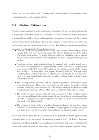
![T =
t0 t−1 .. t2−n t1−n
t1 t0 t−1 .. t2−n
: : : : :
tn−2 .. t1 t0 t−1
tn−1 tn−2 .. t1 t0
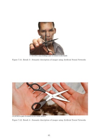
where negative indices were used for convenience of notation.
Now define the operation T = toeplitz(t) as converting a vector t = [t1−n, ...t−1, t0, t1, ..tn−1]
(of length 2∗n−1) to the form shown above, with the negative indices of t corresponding
to the first row of T and the positive indices to the first column, with t0 as the corner
element.
Consider a kxky × kxky matrix T of the form
T =
T0 T−1 .. T1−ky
T1 T0 T−1 :
: : : T−1
Tky−1 .. T1 T0
where each block Tj is a kx × kx Toeplitz matrix. This matrix is called block Toeplitz
with Toeplitz blocks (BTTB). Finally, two-dimensional convolution can be converted to
an equivalent matrix multiplication form:
t ∗ f = mat(Tvec(f))
where T is the kxky × kxky BTTB matrix of the form shown above with Tj =
toeplitz(t.,j). Here t.,j denotes the jth column of the (2kx − 1) × (2ky − 1) matrix
t.
The blur operator is denoted by H. Depending on the image source, the assumption
of blur can be omitted in certain cases. The results obtained for the blur model are as
shown below. Blur has been treated as a Gaussian signal in this case.
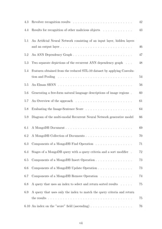
Downsampling
The two-dimensional down-sampling operator discards some elements of a matrix while
leaving others unchanged. In the case of downsampling-by-rows operator, Dx(rx), the
12](https://image.slidesharecdn.com/593f2364-fd42-428c-b3d4-41a7c75ec749-161005015707/85/Final-Report-Major-Project-MAP-23-320.jpg)


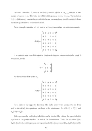
![are then sorted and stored and the most dominant eigen vectors are extracted. Based on
the dimensionality we give,the number of eigen faces is decided.
Training of Eigen Faces
A database of all training and testing images is created. We give the number of training
samples and all those images are then projected over our eigen faces, where the difference
between the image and the centred image is calculated. The new image T is transformed
into its eigenface components (projected into ’face space’) by a simple operation,
wk = µkT
(T − ψ) k = 1, 2....M
The weights obtained above form a vector ΩT
= [w1, w2, w3, ...wM ] that describes the
contribution of each eigen face in representing the input face image. The vector may
then be used in a standard pattern recognition algorithm to find out which of a number
of predefined face class, if any, best describes the face.
Face Recognition Process
The above process is applied to the test image and all the images in the training set. The
test image and the training images are projected over the eigen faces. The differentials
on the various axes for the projected test images over the projected training images is
found out, and based on these results, the Euclidean distance is calculated. Based on the
various Euclidean results calculated, we find the least of them all and the corresponding
class of the training images is given. The recognition index is then divided by total
number of trained images to give the recognized ”class” of the image.
3.3.4 Significance of PCA approach
In PCA approach, we are reducing the dimensionality of face images and are enhanc-
ing the speed for face recognition. We can choose only M’ Eigenvectors with highest
Eigenvalues. Since, the lower Eigenvalues does not provide much information about face
variations in corresponding Eigenvector direction, such small Eigenvalues can be neglected
to further reduce the dimension of face space. This does not affect the success rate much
and is acceptable depending on the application of face recognition. The approach using
Eigen-faces and PCA is quite robust in the treatment of face images with varied facial
expressions as well as directions. It is also quite efficient and simple in the training and
34](https://image.slidesharecdn.com/593f2364-fd42-428c-b3d4-41a7c75ec749-161005015707/85/Final-Report-Major-Project-MAP-45-320.jpg)


![achieved by dividing the image into small connected regions, called cells, and for each cell
compiling a histogram of gradient directions or edge orientations for the pixels within the
cell. The combination of these histograms then represents the descriptor. For improved
accuracy, the local histograms can be contrast-normalized by calculating a measure of
the intensity across a larger region of the image, called a block, and then using this value
to normalize all cells within the block. This normalization results in better invariance to
changes in illumination or shadowing.
The HOG descriptor maintains a few key advantages over other descriptor methods.
Since the HOG descriptor operates on localized cells, the method upholds invariance to
geometric and photometric transformations, except for object orientation. Such changes
would only appear in larger spatial regions. Moreover, as Dalal and Triggs discovered,
coarse spatial sampling, fine orientation sampling, and strong local photometric normal-
ization permits the individual body movement of pedestrians to be ignored so long as
they maintain a roughly upright position. The HOG descriptor is thus particularly suited
for human detection in images.
4.3 Algorithmic Implementation
4.3.1 Gradient Computation
The first step of calculation in many feature detectors in image pre-processing is to ensure
normalized color and gamma values. As Dalal and Triggs point out, however, this step
can be omitted in HOG descriptor computation, as the ensuing descriptor normalization
essentially achieves the same result. Image pre-processing thus provides little impact on
performance. Instead, the first step of calculation is the computation of the gradient
values. The most common method is to simply apply the 1-D centered, point discrete
derivative mask in one or both of the horizontal and vertical directions. Specifically, this
method requires filtering the color or intensity data of the image with the following filter
kernels:
[−1, 0, 1] and [−1, 0, 1]T
Dalal and Triggs tested other, more complex masks, such as 3 × 3 Sobel masks (Sobel
operator) or diagonal masks, but these masks generally exhibited poorer performance in
human image detection experiments. They also experimented with Gaussian smoothing
before applying the derivative mask, but similarly found that omission of any smoothing
38](https://image.slidesharecdn.com/593f2364-fd42-428c-b3d4-41a7c75ec749-161005015707/85/Final-Report-Major-Project-MAP-49-320.jpg)


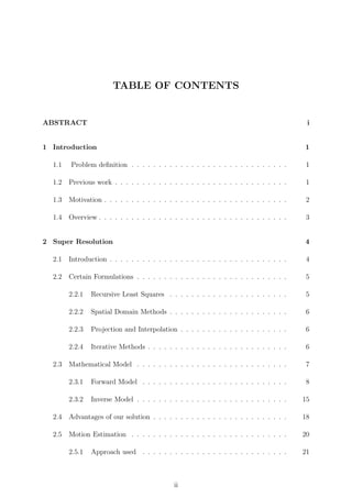
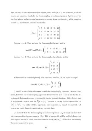
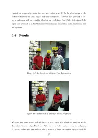
![Figure 5.3: Two separate depictions of the recurrent ANN dependency graph
random variable X. This view is most commonly encountered in the context of graphical
models.
The two views are largely equivalent. In either case, for this particular network archi-
tecture, the components of individual layers are independent of each other (e.g. the
components of g are independent of each other given their input h). This naturally
enables a degree of parallelism in the implementation.
Networks such as the previous one are commonly called feedforward, because their graph
is a directed acyclic graph. Networks with cycles are commonly called recurrent. Such
networks are commonly depicted in the manner shown at the top of the figure, where f
is shown as being dependent upon itself. However, an implied temporal dependence is
not shown.
Learning
What has attracted the most interest in neural networks is the possibility of learning.
Given a specific task to solve, and a class of functions F, learning means using a set of
observations to find f∗
in F which solves the task in some optimal sense. This entails defining a cost function
C : F → R such that, for the optimal solution f∗
, C(f∗
) ≤ C(f) ∀ f ∈ F i.e., no solution
has a cost less than the cost of the optimal solution.
The cost function C is an important concept in learning as it is a measure of how far
away a particular solution is from an optimal solution to the problem to be solved.
Learning algorithms search through the solution space to find a function that has the
smallest possible cost. For applications where the solution is dependent on some data,
the cost must necessarily be a function of the observations, otherwise we would not be
modelling anything related to the data. It is frequently defined as a statistic to which
only approximations can be made. As a simple example, consider the problem of finding
the model f, which minimizes C = E [(f(x) − y)2
], for data pairs (x, y) drawn from some
distribution D. In practical situations we would only have N samples from D and thus,
48](https://image.slidesharecdn.com/593f2364-fd42-428c-b3d4-41a7c75ec749-161005015707/85/Final-Report-Major-Project-MAP-59-320.jpg)


![(1 + e−x
)−1
. The advantage of ReLU compared to tanh units is that with it, the neural
network trains several times faster.
Pooling Layer
In order to reduce variance, pooling layers compute the maximum or average value of a
particular feature over a region of the image. This will ensure that the same result will
be obtained, even when image features have small translations. This is an important
operation for object classification and detection.
Dropout Layer
Since a fully connected layer occupies most of the parameters, over-fitting can happen
easily. The dropout method is introduced to prevent over-fitting. Dropout also signifi-
cantly improves the speed of training. This makes model combination practical, even for
deep neural nets. Dropout is performed randomly. In the input layer, the probability
of dropping a neuron is between 0.5 and 1, while in the hidden layers, a probability of
0.5 is used. The neurons that are dropped out, will not contribute to the forward pass
and back propagation. This is equivalent to decreasing the number of neurons. This will
create neural networks with different architectures, but all of those networks will share
the same weights.
The biggest contribution of the dropout method is that, although it effectively generates
2n
neural nets, with different architectures (n =number of ”droppable” neurons), and
as such, allows for model combination, at test time, only a single network needs to be
tested. This is accomplished by performing the test with the un-thinned network, while
multiplying the output weights of each neuron with the probability of that neuron being
retained (i.e. not dropped out).
Loss Layer
It can use different loss functions for different tasks. Softmax loss is used for predicting
a single class of K mutually exclusive classes. Sigmoid cross-entropy loss is used for
predicting K independent probability values in [0,1]. Euclidean loss is used for regressing
to real-valued lables [-inf,inf]
52](https://image.slidesharecdn.com/593f2364-fd42-428c-b3d4-41a7c75ec749-161005015707/85/Final-Report-Major-Project-MAP-63-320.jpg)


![representations so that semantically similar concepts across the two modalities occupy
nearby regions of the space.
The idea and the mathematics behind the model are currently being looked into and a
preliminary analysis of the same has been presented below:
Representing Images
Following prior work, we observe that sentence descriptions make frequent references to
objects and their attributes. Thus, we follow the method of Girshick et al. to detect
objects in every image with a Region Convolutional Neural Network (RCNN). The CNN
is pre-trained on ImageNet and fine tuned on the 200 classes of the ImageNet Detection
Challenge. To establish fair comparisons to Karpathy et al., we use the top 19 detected
locations and the whole image and compute the representations based on the pixels Ib
inside each bounding box as follows:
v = Wm[CNNθc (Ib)] + bm
where CNN(Ib) transforms the pixels inside the bounding box Ib into 4096-dimensional
activations of the fully connected layer immediately before the classifier. The CNN pa-
rameters θc contain approximately 60 million parameters and the architecture closely
follows the network of Krizhevsky et al. The matrix Wm has dimensions h × 4096, where
h is the size of the multi-modal embedding space (h currently ranges from 1000-1600
in our experiments). Every image is thus represented as a set of h-dimensional vectors
vi|i = 1...20
Representing Sentences
To establish the inter-modal relationships, we would like to represent the words in the
sentence in the same h-dimensional embedding space that the image regions occupy. The
simplest approach might be to project every individual word directly into this embedding.
However, this approach does not consider any ordering and word context information in
the sentence. An extension to this idea is to use word bi-grams, or dependency tree
relations as previously proposed. However, this still imposes an arbitrary maximum size
of the context window and requires the use of Dependency Tree Parsers that might be
trained on unrelated text corpora.
To address these concerns, we look towards using a bidirectional recurrent neural network
(BRNN) to compute the word representations. In our setting, the BRNN takes a sequence
of N words (encoded in a 1-of-k representation) and transforms each one into an h-
dimensional vector. However, the representation of each word is enriched by a variably-
62](https://image.slidesharecdn.com/593f2364-fd42-428c-b3d4-41a7c75ec749-161005015707/85/Final-Report-Major-Project-MAP-73-320.jpg)

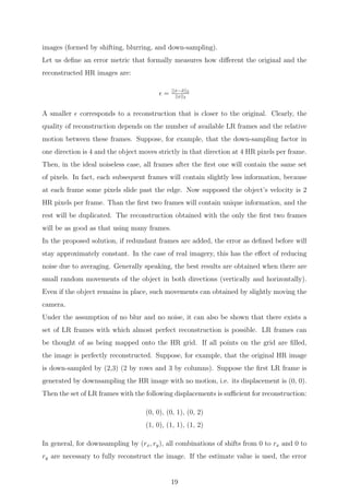
![Figure 5.8: Evaluating the Image-Sentence Score
confident support in the image. In Karpathy et al., they interpreted the dot product vT
i st
between an image fragment i and a sentence fragment t as a measure of similarity and
used these to define the score between image k and sentence l as:
Skl = Σt∈gl
Σi∈gk
max(0, vT
i st)
Here, gk is the set of image fragments in image k and gl is the set of sentence fragments
in sentence l. The indices k, l range over the images and sentences in the training set.
Together with their additional Multiple Instance Learning objective, this score carries the
interpretation that a sentence fragment aligns to a subset of the image regions whenever
the dot product is positive. We found that the following reformulation simplifies the
model and alleviates the need for additional objectives and their hyper-parameters:
Skl = Σt∈gl
maxi∈gk
vT
i st
Here, every word st aligns to the single best image region. As we show in the experiments,
this simplified model also leads to improvements in the final ranking performance. As-
suming that k = l denotes a corresponding image and sentence pair, the final max-margin,
structured loss remains:
C(θ) = Σk[Σlmax(0, Skl − Skk + 1) + Σlmax(0, Slk − Skk + 1)]
This objective encourages aligned image-sentences pairs to have a higher score than mis-
aligned pairs, by a margin.
Decoding text segment alignments to images
64](https://image.slidesharecdn.com/593f2364-fd42-428c-b3d4-41a7c75ec749-161005015707/85/Final-Report-Major-Project-MAP-75-320.jpg)
![Consider an image from the training set and its corresponding sentence. We can interpret
the quantity vT
i st as the un-normalized log probability of the tth
word describing any of the
bounding boxes in the image. However, since we are ultimately interested in generating
snippets of text instead of single words, we would like to align extended, contiguous
sequences of words to a single bounding box. Note that the nave solution that assigns
each word independently to the highest-scoring region is insufficient because it leads to
words getting scattered inconsistently to different regions.
To address this issue, we treat the true alignments as latent variables in a Markov Random
Field (MRF) where the binary interactions between neighbouring words encourage an
alignment to the same region. Concretely, given a sentence with N words and an image
with M bounding boxes, we introduce the latent alignment variables aj ∈ 1...M for
j = 1...N and formulate an MRF in a chain structure along the sentence as follows:
E(a) = Σj=1...N ψU
j (aj) + Σj=1..N−1ψB
j (aj, aj+1)
ψU
j (aj = t) = vT
i st
ψB
j (aj, aj+1) = βπ[aj = aj+1]
Here, β is a hyperparameter that controls the affinity towards longer word phrases. This
parameter allows us to interpolate between single-word alignments (β = 0) and aligning
the entire sentence to a single, maximally scoring region when β is large. We minimize
the energy to find the best alignments a using dynamic programming. The output of this
process is a set of image regions annotated with segments of text.
Idea of a Multi-Modal RNN for generating descriptions
In this section, we assume an input set of images and their textual descriptions. These
could be full images and their sentence descriptions, or regions and text snippets as dis-
cussed in previous sections. The key challenge is in the design of a model that can predict
a variable-sized sequence of outputs. In previously developed language models based on
Recurrent Neural Networks (RNNs), this is achieved by defining a probability distribu-
tion of the next word in a sequence, given the current word and context from previous
time steps. We explore a simple but effective extension that additionally conditions the
generative process on the content of an input image. More formally, the RNN takes the
image pixels I and a sequence of input vectors (x1, ..., xT ). It then computes a sequence
65](https://image.slidesharecdn.com/593f2364-fd42-428c-b3d4-41a7c75ec749-161005015707/85/Final-Report-Major-Project-MAP-76-320.jpg)
![Figure 5.9: Diagram of the multi-modal Recurrent Neural Network generative model
of hidden states (h1, ..., ht) and a sequence of outputs (y1, ..., yt) by iterating the following
recurrence relation for t = 1toT:
bv = Whi[CNNθc (I)]
ht = f(Whxxt + Whhht1 + bh + bv)
yt = softmax(Wohht + bo)
In the equations above, Whi, Whx, Whh, Woh and bh, bo are a set of learnable weights
and biases. The output vector yt has the size of the word dictionary and one additional
dimension for a special END token that terminates the generative process. Note that we
provide the image context vector bv to the RNN at every iteration so that it does not
have to remember the image content while generating words.
RNN Training
The RNN is trained to combine a word (xt), the previous context (ht1) and the image
information (bv) to predict the next word (yt). Concretely, the training proceeds as follows
(refer the above figure): We set h0 = 0, x1 to a special START vector, and the desired
label y1 as the first word in the sequence. In particular, we use the word embedding for
the as the START vector x1. Analogously, we set x2 to the word vector of the first word
and expect the network to predict the second word, etc. Finally, on the last step when
xT represents the last word, the target label is set to a special END token. The cost
function is to maximize the log probability assigned to the target labels.
RNN Testing
The RNN predicts a sentence as follows: We compute the representation of the image bv,
set h0 = 0, x1 to the embedding of the word the, and compute the distribution over the
first word y1. We sample from the distribution (or pick the argmax), set its embedding
vector as x2, and repeat this process until the END token is generated.
66](https://image.slidesharecdn.com/593f2364-fd42-428c-b3d4-41a7c75ec749-161005015707/85/Final-Report-Major-Project-MAP-77-320.jpg)


![REFERENCES
[1] http://news.bbc.co.uk/2/hi/science/nature/1953770.stm
[2] http://www.wired.com/2008/02/predicting-terr/
[3] TGPM: Terrorist Group Prediction Model for Counter Terrorism, Abhishek Sachan
and Devshri Roy, Computer Science Maulana Azad National Institute of Technology
Bhopal, India
[4] Super Resolution Techniques by Martin Vetterli and group at LCAV, EPFL
[5] MAROB (Minorities at Risk Organizational Behaviour) Database for Verification
[6] Computational Analysis of Terrorist Groups: Lashkar-e-Taiba, V.S. Subrahmanian,
Aaron Mannes, Amy Sliva, Jana Shakarian, John Dickerson, University of Maryland
[7] Terrorist Organization Behavior Prediction Algorithm Based on Context Subspace,
Anrong Xue, Wei Wang, and Mingcai Zhang, School of Computer Science and
Telecommunication Engineering, Jiangsu University
[8] IMDB - Person of Interest, CBS Network
[9] IMDB - Source Code, Summit Entertainment
[10] A Spatial Clustering Method With Edge Weighting for Image Segmentation, Nan
Li, Hong Huo ; Yu-ming Zhao ; Xi Chen ; Tao Fang, Dept. of Automation, Shanghai
Jiao Tong Univ., Shanghai, China
[11] Machine Learning in Multi-frame Image Super-resolution, Lyndsey C Pickup,
Robotics Research Group, Department of Engineering Science, University of Oxford
[12] Super-resolution in image sequences, Andrey Krokhin, Department of Electrical and
Computer Engineering, Northeastern University, Boston, Massachusetts
[13] Efficient Activity Detection with Max-Subgraph Search, Chao-Yeh Chen and Kristen
Grauman, University of Texas at Austin
93](https://image.slidesharecdn.com/593f2364-fd42-428c-b3d4-41a7c75ec749-161005015707/85/Final-Report-Major-Project-MAP-104-320.jpg)
![[14] Detecting Unusual Activity in Video, Hua Zhong, Carnegie Mellon University, Jianbo
Shi Mirk Visontai, University of Pennsylvania
[15] Online Detection of Unusual Events in Videos via Dynamic Sparse Coding, Bin Zhao,
Carnegie Mellon University, Li Fei-Fei, Stanford University, Eric P. Xing, Carnegie
Mellon University
[16] Human Activity Clustering for Online Anomaly Detection, Xudong Zhu, Zhijing Liu,
Juehui Zhang, University of Xidian, Xi’an, China
[17] Human Activity Detection and Recognition for Video Surveillance, Wei Niu, Jiao
Long, Dan Han, and Yuan-Fang Wang, Department of Computer Science, University
of California
[18] Group Event Detection for Video Surveillance, Weiyao Lin, Ming-Ting Sun, Radha
Poovendran, University of Washington, Seattle, USA, Zhengyou Zhang, Microsoft
Coop., Redmond, USA
[19] A Constrained Probabilistic Petri Net Framework for Human Activity Detection
in Video, Massimiliano Albanese, Rama Chellappa, Vincenzo Moscato, Antonio Pi-
cariello, V. S. Subrahmanian, Pavan Turaga, Octavian Udrea
[20] Activity Understanding and Unusual Event Detection in Surveillance Videos Chen
Change Loy, Queen Mary University of London
[21] Unsupervised learning approach for abnormal event detection in surveillance video
by revealing infrequent patterns, Tushar Sandhan and Jin Young Choi, Seoul Na-
tional University,Tushar Srivastava and Amit Sethi, Indian Institute of Technology,
Guwahati
[22] Co-clustering documents and words using Bipartite Spectral Graph Partitioning,
Inderjit S. Dhillon, Department of Computer Sciences, University of Texas, Austin
[23] Knowledge Discovery By Spatial Clustering Based on Self-Organizing Feature Map
and a Composite Distance Measure, Limin Jiao, Yaolin Liu, School of Resource and
Environment Science, Wuhan University
[24] Deep Visual-Semantic Alignments for Generating Image Descriptions by Andrej
Karpathy and Li Fei-Fei, Department of Computer Science, Stanford University
94](https://image.slidesharecdn.com/593f2364-fd42-428c-b3d4-41a7c75ec749-161005015707/85/Final-Report-Major-Project-MAP-105-320.jpg)

This document summarizes a student project on predicting malicious activity using real-time video surveillance. The project applies techniques like super-resolution, face and object recognition using HOG features, and neural networks to enhance video quality, identify objects and faces, and semantically describe scenes to detect unusual activity. Algorithms were implemented in MATLAB and results were stored in a MongoDB database. Key techniques included super-resolution, PCA-based face recognition, HOG-based object detection, and neural networks like CNNs and RNNs for image captioning. The project aims to help detect criminal activity and track convicted individuals in public spaces.