Estimating the pointof visual focus on the screen
to make avatars show visual focus in virtual meeting situations.
By
Per Nystedt
Master’s thesis in Computer Science (20 credits)
2.
Abstract
This master’s thesisinvestigates the possibility of estimating the user’s point
of visual focus on the screen to make an avatar show the user’s visual focus.
The user in this case is a person who participates in a virtual environment
meeting.
Two systems have been implemented, both use low-resolution video images,
which make them non-intrusive. Both systems run in real-time. The first
system is based on a traditional eye gaze tracking technique. A light source
generates a specular highlight in the eye. The second system is based on
artificial neural networks. Both systems allow the user to pan and tilt his/her
head.
The mean error estimating the position of visual focus was 1.7° for the first
system and 3.06° (best result 1.36°) for the second system.
Bestämning av visuellt fokus på skärmen
För att styra en avatars uppmärksamhet i virtuella mötessituationer.
Sammanfattning
Detta examensarbete undersöker möjligheten att bestämma den punkt på
skärmen på vilken användaren tittar för att styra en avatars visuella fokus.
Användaren i detta fall är en person som medverkar i ett virtuellt möte.
Två system har implementerats, båda använder sig av lågupplösande
videobilder, vilket gör att de inte är i kontakt med användaren. Båda
systemen fungerar i realtid. Det första systemet är baserat på en traditionell
“eye gaze tracking”-teknik. En ljuskälla skapar en reflex i ögat. Det andra
systemet är baserat på artificiella neuronnät. Båda systemen fungerar även
om användaren vrider på huvudet.
Medelfelet vid bestämning av position för visuellt fokus är 1.7° i det första
systemet och 3.06° (bästa resultat 1.36°) i det andra systemet.
1
3.
Preface
This master’s thesiswas performed at Telia Research AB, Farsta, Sweden.
Acknowledgements
I would like to thank my tutor Thomas Uhlin (Ph.D) at Telia Research AB
for good and interesting ideas concerning both the implementation and the
structure of this report. I also would like to thank Jörgen Björkner for all
those late hours helping me with sockets (connecting the application with
virtual meeting application) and interesting discussions concerning the
implementation. I especially want to thank Martin Jonsson, my roommate,
for being such a nice fellow with lots of good ideas and time to discuss his
work and mine. Last of all I would like to thank all others that have been
around.
My tutor at KTH has been Stefan Carlsson whom I also would like to thank.
2
4.
1 INTRODUCTION.................................................................................................................. 5
1.1PROBLEM DEFINITION ...................................................................................................... 6
1.2 RELATED WORK............................................................................................................... 7
1.3 HOW TO READ THIS REPORT ............................................................................................. 8
2 BASICS ................................................................................................................................. 10
2.1 THE ARCHITECTURE OF THE EYE .................................................................................... 10
2.2 DEFINITIONS .................................................................................................................. 11
2.3 CHROMATIC COLORS...................................................................................................... 11
2.4 ARTIFICIAL NEURAL NETWORKS .................................................................................... 12
3 SYSTEM OVERVIEW........................................................................................................ 15
3.1 EXTRACTING FACIAL DETAILS (MAIN STEP #1).............................................................. 16
3.1.1 Adapting the skin-color definition............................................................................ 17
3.1.2 Detecting and tracking the face ............................................................................... 18
3.1.3 Detecting and tracking the eyes and nostrils ........................................................... 19
3.2 PROCESSING EXTRACTED DATA TO FIND POINT OF VISUAL FOCUS (MAIN STEP # 2) ....... 20
3.2.1 Using the position of the corneal reflection and the limbus..................................... 20
3.2.2 Using an artificial neural network........................................................................... 21
3.3 HARDWARE ................................................................................................................... 22
3.4 SYSTEM PREPARATION................................................................................................... 22
3.4.1 Using the positions of the corneal reflection and the limbus................................... 23
3.4.2 Using an artificial neural network........................................................................... 23
4 DETECTING AND TRACKING THE FACE .................................................................. 25
4.1 ADAPTING THE SKIN-COLOR DEFINITION........................................................................ 25
4.1.1 Facial details not known .......................................................................................... 25
4.1.2 Facial details known ................................................................................................ 27
4.2 SEARCH AREAS FOR THE FACE ....................................................................................... 28
4.2.1 Detecting the face..................................................................................................... 28
4.2.2 Tracking the face...................................................................................................... 28
4.3 SEARCHING PROCEDURE FOR THE FACE ......................................................................... 29
4.4 TESTING THE GEOMETRY OF THE FACE........................................................................... 30
5 DETECTING AND TRACKING THE EYES AND NOSTRILS.................................... 31
5.1 EYES AND NOSTRILS FEATURES...................................................................................... 31
5.2 SEARCH AREAS FOR THE FACIAL DETAILS ...................................................................... 31
5.2.1 Detecting the facial details....................................................................................... 32
5.2.2 Tracking the facial details........................................................................................ 35
5.3 SEARCHING PROCEDURE FOR THE FACIAL DETAILS ........................................................ 37
5.4 TESTING THE FACIAL DETAILS........................................................................................ 38
5.5 IMPROVING THE POSITION OF THE EYES.......................................................................... 39
6 PROCESSING EXTRACTED DATA TO FIND POINT OF VISUAL FOCUS............ 41
6.1 USING THE POSITIONS OF THE CORNEAL REFLECTION AND THE LIMBUS ......................... 41
6.1.1 Finding the specular highlight................................................................................. 42
6.1.2 Preprocessing the eye images .................................................................................. 43
6.1.3 Estimating the point of visual focus ......................................................................... 47
6.2 USING AN ARTIFICIAL NEURAL NETWORK ...................................................................... 49
6.2.1 Preprocessing the eye images .................................................................................. 50
6.2.2 Estimating the point of visual focus ......................................................................... 51
7 ANN ARCHITECTURE DESCRIPTION......................................................................... 53
3
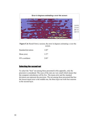
5.
7.1 FIRST NEURALNET.........................................................................................................53
7.2 SECOND NEURAL NET.....................................................................................................54
8 IMPLEMENTATION JUSTIFICATION..........................................................................56
8.1 CHOICE OF EYE GAZE TRACKING TECHNIQUE ................................................................56
8.1.1 System requirements.................................................................................................56
8.1.2 Selecting the techniques ...........................................................................................58
8.2 DETECTING AND TRACKING THE FACE............................................................................59
8.2.1 Adapting the skin-color definition............................................................................59
8.2.2 Search areas.............................................................................................................60
8.2.3 Search procedure .....................................................................................................63
8.3 DETECTING AND TRACKING THE EYES AND NOSTRILS ....................................................63
8.3.1 Eyes and nostrils features ........................................................................................64
8.3.2 Search areas.............................................................................................................65
8.3.3 Search procedure .....................................................................................................65
8.3.4 Testing the facial details ..........................................................................................66
8.3.5 Improving the position of the eyes............................................................................66
8.4 USING THE POSITIONS OF THE CORNEAL REFLECTION AND THE LIMBUS .........................66
8.4.1 Preprocessing the eye images ..................................................................................67
8.4.2 Estimating the point of visual focus .........................................................................68
8.5 USING AN ARTIFICIAL NEURAL NETWORK ......................................................................69
8.5.1 Preprocessing the eye images ..................................................................................70
8.6 ANN IMPLEMENTATION.................................................................................................70
8.6.1 Discussion ................................................................................................................70
8.6.2 Architecture..............................................................................................................72
9 TRAINING/CALIBRATING THE SYSTEMS.................................................................74
9.1 CORNEAL REFLECTION BASED SYSTEM ..........................................................................74
9.2 ANN BASED SYSTEM .....................................................................................................74
10 RESULTS..............................................................................................................................76
10.1 CORNEAL REFLECTION BASED SYSTEM ..........................................................................76
10.2 ANN BASED SYSTEM .....................................................................................................77
11 CONCLUSION.....................................................................................................................79
11.1 CORNEAL REFLECTION BASED SYSTEM ..........................................................................79
11.2 ANN BASED SYSTEM .....................................................................................................80
12 FUTURE IMPROVEMENTS .............................................................................................82
12.1 EXTRACTING FACIAL DETAILS........................................................................................82
12.2 PROCESSING EXTRACTED DATA TO FIND POINT OF VISUAL FOCUS ..................................82
12.2.1 Corneal reflection based system..........................................................................82
12.2.2 ANN based system ...............................................................................................83
REFERENCES...............................................................................................................................84
APPENDIX A - EYE GAZE TRACKING TECHNIQUES .....................................................86
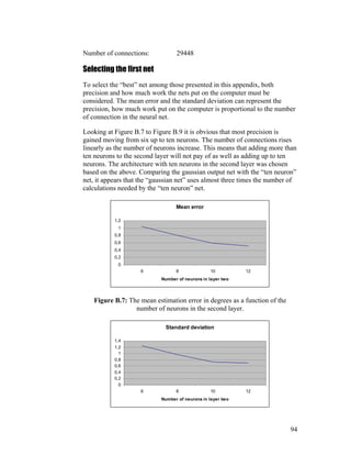
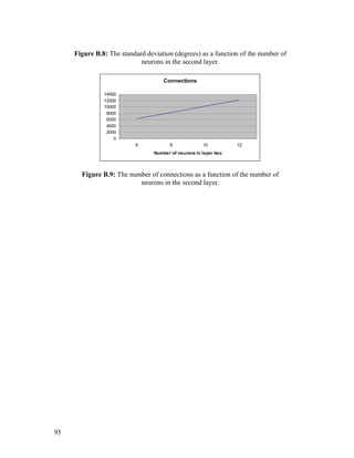
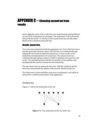
APPENDIX B – CHOOSING FIRST NET FROM RESULTS................................................90
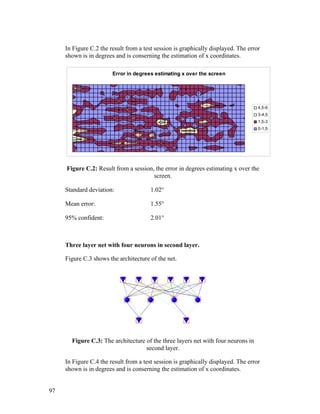
APPENDIX C – CHOOSING SECOND NET FROM RESULTS ..........................................96
4
6.
1 Introduction
We useto think of our eyes mainly as input-organs, organs that observe the
surroundings. This is also their most important role, but in fact they also
operate as output-organs. The output they are producing is the direction in
which we are looking, thus indicating what is being focused upon. As Argyle
writes in “Bodily communication” [1], “Gaze, or looking, is of central
importance in social behavior”.
In collaborative virtual meeting-places the participants are being represented
by graphical objects, so called avatars. Figure 1.1 shows three views of the
same virtual meeting situation, three avatars sitting around a desk. One
problem with the avatars of today is that they don’t conduct facial
expressions nor show the other participants where the person who is
represented has his/her focus. It’s easy to understand that problems
concerning who addresses whom easily occur in a multi participant meeting.
To solve the problem with who is addressing whom, the avatar should face
the same object/avatar as his/her owner (the participant represented by the
avatar) focuses upon at the screen. Making the avatar pan or tilt its head is
easy, it is acquiring the information to make it act correctly that is the main
problem.
Figure 1.1 shows three snapshots from a virtual meeting situation where the
problem with visual focus has been solved by using the system described in
this report. The avatar sitting unaccompanied addresses the avatar sitting to
the left of “him” by just looking at his avatar on the screen, left avatar, upper
left image.
5
7.
Figure 1.1: Threeviews from a virtual meeting situation. The system in this report
makes the avatars able to show visual focus.
Figure 1.2 shows the views of the persons sitting at the same side of the table
in Figure 1.1.
Figure 1.2: The views of the persons (avatars) sitting at the same side of the table
in Figure 1.1.
This master’s thesis investigates the possibility of making an avatar show
visual focus. The focus of the avatar is to be controlled by finding the point
on which the user focuses upon at the screen. The user in this case is a person
who participates in a virtual environment meeting.
1.1 Problem definition
The object of my work was to:
• estimate where a virtual environment meetings application user has his/her
point of visual focus on the screen, do this with a video camera and a computer
• estimate the accuracy with which the visual focus tracking should be done
facing user face mobility
• implement a real-time system and integrate it with existing virtual environment
meetings application.
6
8.
1.2 Related work
Inthis section some related work that has been studied will be presented.
In the paper [2] by Roel Vertegaal et al. they discuss why, in designing
mediated systems, focus should first be placed on non-verbal cues, which are
less redundantly coded in speech than those normally conveyed by video.
This paper is related to [3].
Roel Vertgaal et al. [3] have developed a system where a commercial eye
gaze tracker was used for bringing the point of visual focus into the virtual
environment. The goal was mainly to organize different aspects of awareness
into an analytic framework and to bring those aspects of awareness into a
virtual meeting room.
To find appropriate eye gaze tracking techniques a large number of articles
were studied among them “Eye Controlled Media: Present and future State”
[4] by Arne John Glenstrup and Theo Engell-Nielsen where most techniques
are mentioned. The report [4] has an information psychology based approach.
When the appropriate techniques were found, my task was divided into two
parts, finding the facial details and processing the extracted data to find point
of visual focus. Articles studied to implement the facial detail extraction part.
Gaze Tracking for Multimodal Human-Computer Interaction [5] by Rainer
Stiefelhagen uses color information to find the face and intensities to find the
details.
Jie Yang and Alex Waibel uses a stochastical model (skin-color) for tracking
faces described in [6].
Kin Chong Yow and Roberto Cipolla describe in [7] how faces can be
located through finding facial features. The method uses a family of Gaussian
derivative filters to search and extract the features.
S.Gong et al. describe in [8] how faces can be found through fitting an ellipse
to temporal changes. A Kalman filter is applied to model the dynamics of the
ellipse parameters.
James L. Crowley and Francois Berard describe in [9] how faces can be
detected “from blinking” and from color information.
Saad Ahmed Sirohey shows in [10] that faces can be detected by fitting an
ellipse to the image edge map.
In [11] Jörgen Björkner has implemented a number of methods to detect the
face. The facial details are found using either gray levels or eye blinks.
7
9.
Martin Hunke andAlex Waibel combine color information with movement
and an artificial neural network to detect faces in [12].
Carlos Morimoto et al. uses the “bright eye effect” known from taking
pictures using a flash to locate eyes and faces. This is described in [13].
Articles studied to implement the data processing part:
Shumeet Baluja and Dean Pomerleau show in [14] that the point of visual
focus can be estimated non-intrusively by an artificial neural network. The
same thing is done by Rainer Stiefelhagen, Jie Yand and Alex Waibel in [15]
and Alex Christian Varchim, Robert Rae and Helge Ritter in [16].
1.3 How to read this report
The aim of this section is to make the report easier to read and to make the
reader read only the parts interesting for him/her.
The report is divided into five main parts
1. Basics (Chapter 2)
2. System overview (Chapter 3)
3. Details about the implementation (Chapter 4 - 7, 9)
4. Implementation justifications (Chapter 8)
5. Results, conclusions and future improvements (Chapter 10 - 12)
Part 1, Basics consists of useful fundamental information within the
concerned area. This is a part that should be briefly read if not well known to
the reader.
Part 2, System overview shows the overall relationship among all the
elements described in this report, useful to read and understand before going
any further. Readers who are interested in image processing parts only can
skip this part.
Part 3, details about the implementation describes the implementation in a
way that the system components can be re-created by the reader. It is not
necessary to read this part to understand the concept of the system.
Part 4, implementation justifications informs about why the system is built
the way it’s built and why the different selections of methods and algorithms
8
10.
were made. Thispart can be read simultaneously with Part 2 or Part 3 or
skipped.
Part 5, results, conclusions and further research consists of the outcome of
the work done. Results are to be read by reader who wants to compare
different methods or results from others. Conclusions and further research
consists of the experience gained from this work, maybe useful for reader
who wants to develop own systems.
9
11.
2 Basics
In thischapter some basics that are useful to know reading this report are
presented.
2.1 The architecture of the eye
In Figure 2.1 some of the most important parts of the eye are shown.
Pupil: The opening in the center of iris.
Sclera: The white hard tissue.
Iris: The area that gives the eye its color.
Lens: The transparent structure behind the pupil.
Cornea: The outermost layer, protecting the eye.
Limbus: The visual border, connecting the iris and the sclera.
Retina: The area inside the eyeball that is sensitive to light.
Limbus
Pupil
Cornea
Retina
Lens
Optical nerve
Sclera
Iris
Figure 2.1: The most important parts of the eye.
10
12.
2.2 Definitions
In thissection some definitions are stated, these are useful be familiar with
when reading this report.
Point of visual focus: The point on which the subject’s eyes are turned
toward (not necessarily making attention to).
Avatar: [17]”A graphical icon that represents a real person in a cyberspace
system”. [18] ”In the Hindu religion, an avatar is an incarnation of a deity;
hence, an embodiment or manifestation of an idea or greater reality.”
Virtual environment: A computer generated location with non-real spatial
presence.
Detecting: Finding an object without knowing its past concerning size and
location.
Tracking: The opposite of detecting, finding an object knowing something
about where it was before.
2.3 Chromatic colors
Chromatic colors are used in this work for detecting and tracking the face.
It has been recognized that although skin-color appears to vary over a wide
range, the difference is not so much in color as in brightness. The color
distribution of the skin-color is therefore clustered in a small area of the
chromatic color space.
If R,G and B are the red, green and blue color components of an image
segment, chromatic colors will be defined by the normalization shown in
Definition 2.1.
BGR
B
b
BGR
G
g
BGR
R
r
++
=
++
=
++
=
Definition 2.1: The definition of chromatic colors.
Since r + g + b = 1, b is redundant.
11
13.
Figure 2.2 showsthe transformation between the RGB and the chromatic
color space.
B=1
B
R
G
B
G
R
(R,G,B)
(r,g)
RGB-color space Chromatic-color space
Figure 2.2: RGB to chromatic color transformation.
2.4 Artificial neural networks
There is no generally accepted definition of an artificial neural network
(ANN). But the general opinion seams to be that an ANN is a network of
many simple processors (“units”), each having a small amount of local
memory. Communication channels (“connections”) which carry data connect
the units. The units operate only on their local data and on the inputs they
receive via the connections.
Most ANNs must be trained to work satisfying. This is accomplished using a
“training” rule and a set of training data. The training data are examples
along with the “right answer”. The training procedure adjusts the weights of
the connections on the basis of the training data. Some sort of general
representation of the features in the training data is stored within the ANN,
which means that data never exposed to the ANN can be successfully
processed. The most usual training “rule” is back-propagation, which is done
in two steps. First the inputs are sent forward through the network to produce
an output. Then the difference between the actual and desired outputs
produces error signals that are sent “backwards” through the network to
modify the weights.
The ANN architecture determines how the processing units are connected.
The most commonly used architecture is feed-forward which means that for
every exposure of new input data to the ANN the processing units never
participate more than once in the process. In feed-forward architectures,
processing units are organized into different layers, input layer, one or more
hidden layers and an output layer. Figure 2.3 shows a feed-forward three
layer ANN with a bias input.
12
14.
Unit 1 Unit2 Bias
Unit 3 Unit 4
Unit 5
Input 1 Input 2
Input layer
Hidden layer
Output layer
Figure 2.3: An example of a feed-forward three layer net with bias input.
The processing units are called neurons. Neurons consist of different
elements:
1. Connections, which include a bias input.
2. State function (normally summation function)
3. Function (nonlinear)
4. Output
The elements can be seen in Figure 2.4.
1. Connections
4. Output
2. State function
3. Function
Figure 2.4: The elements of a neuron.
Input connections have an input value that is either received from the
previous neuron or in the case of the input layer from the outside. A weight is
a real number that represents the amount of the neuron output value that
reaches the connected neuron input.
13
15.
The most commonstate function is a summation function. The output of the
state function becomes the input for the transfer function.
The transfer function is a nonlinear mathematical function used to convert
data to a specific scale. There are two basic types of transfer functions:
continuous and discrete. Commonly used continuous functions used are
ramp, sigmoid, arc tangent and hyperbolic tangent.
14
16.
3 System overview
Thesystem in this report estimates the user point of visual focus on the
screen. This chapter describes the process that takes place every time a new
frame is grabbed. Figure 3.1 shows the main process. The implementation
includes the boxes drawn with continuous lines, boxes drawn with dashed
lines imply existing applications. The appearance of the user is captured by a
video camera.
Extracting facial details
(Main step #1)
Processing extracted data
to estimate point of visual
focus on the screen
(Main step #2)
Fail
Virtual environment
meetings application
Result
Grab a new frame
Figure 3.1: The main process that takes place every new frame.
15
17.
3.1 Extracting facialdetails (Main step #1)
The first step in the main process shown in Figure 3.1, is to extract the facial
details, eyes and nostrils. This step consists of smaller processing units. In
Figure 3.2 these units are shown with the relation among them. The dashed
boxes indicate to what chapter and to what part of the implementation that
the units belong. The details about the processing units are found in Chapter
4 and Chapter 5, “Detecting and tracking the face” and “Detecting and
tracking the eyes and nostrils”, the motives and justifications in Section 8.2
and Section 8.3.
The eyes and nostrils are found either within the face region or around the
positions they were found at in the previous frame. The face region is found
through searching for a large skin-colored area. The eyes and nostrils are
found through searching for specific eye and nostril features.
16
18.
Is there any
information
aboutthe facial
details from the
previous
frame?
Check face
height and
width relation,
is it possible
it’s a face?
Are the
positions of the
eyes and
nostrils fulfilling
the geometrical
test?
Is there any
information
about the face
from the
previous
frame?
Face tracking:
Locate the new face
by using information
about location of the
previous face.
Detail tracking:
Search for eyes and
nostrils in areas
around previous
positions
Detail detection:
Search for eyes and
nostrils in areas
based on the face
size and position
Make a color
sample on the most
probable skin-
colored area
Face detection:
Locate the face by
finding the largest
skin-colored area.
Make color-
sample in known
face region
YES
NO
YES
YES
YES
NO
NO
NO
Enhance the positions
of the eyes
Construct a face
around the eyes and
nostrils
Fail
Adapting the skin-color
definition
Detecting and
tracking the eyes
and nostrils
Detecting and
tracking the face
Main step #1
Figure 3.2: Units within “Extracting facial details”.
3.1.1 Adapting the skin-color definition
The details about the processing units in “Adapting the skin-color definition”
are found in Section 4.1, “Adapting the skin-color definition ”, the motives
and justifications in Section 8.2.1, with the same name. In Figure 3.2, the
relationship between the processing units in “Adapting the skin-color
definition” and the rest of the units in “Extracting facial details” can be seen.
As can be seen in Figure 3.2, “Adapting the skin-color definition is a part of
“Detecting and tracking the face”.
17
19.
The skin-color definitionsconsists of a color vector C =(r,g) of chromatic
colors and a threshold difference V. Chromatic colors are explained in
Section 2.3. The adaption of the skin-color definition procedure adapts the
color vector C to the specific skin-color of the user by making a sample of
the skin.
If the location of the face is known, a color sample is made within the face. If
the location is not known, the most probable area based on default skin-color
will be sampled. In Figure 3.3 it can bee seen how the definition of skin-color
has changed as a sample of the skin has been taken.
r
g
r
g
Adapt skin-
color definition
Default skin-colors Adapted skin-colors
Figure 3.3: The new skin-color definition is shown to the right.
Figure 3.4 shows threshold images, white areas signify colors within the
skin-color definition. In the middle image the default skin-color definition is
used when thresholding the original image. In the image to the right the
adjusted skin-color definition is used. The left most image shows the original
image.
Figure 3.4: (left) Original image. (middle) Threshold with default skin-color
definition. (right) Threshold after adapting skin-color definition.
3.1.2 Detecting and tracking the face
The details about the processing units in “Detecting and tracking the face”
are found in Chapter 4, “Detecting and tracking the face ”, the motives and
justifications in Section 8.2, with the same name. In Figure 3.2, the
18
20.
relationship between theprocessing units in “Detecting and tracking the
face” and the rest of the processing units in “Extracting facial details” can be
seen.
The skin-color definition, see previous section is used for classifying the
pixels within the search area. They are either skin-colored or not, see Figure
3.5 to the right. The face is given by the rectangle circumfering an area with
a skin-color density above a certain threshold. Figure 3.5 shows the
circumfered area in both the original and the threshold image.
Figure 3.5: (left) Original image with detected face area marked. (right) Threshold
image, white indicates skin-color. The face area is marked by the rectangle.
The area searched for the face depends on whether the location of the face
successfully could be established in the previous frame. If the face was
located, an area slightly larger than the previously found face will be
searched; this is called tracking. If not, the entire image will be searched; this
is called detecting. See Figure 3.2 for overview and Section 4.2 for detailed
information about search areas.
A geometrical test is conducted to decide whether the found area is likely to
be a face or not. For example, a head that has a greater width than it has
height will generate fail, see Section 4.4 for detailed information.
3.1.3 Detecting and tracking the eyes and nostrils
The details about the processing units in “Detecting and tracking the eyes
and nostrils” are found in Chapter 5, the motives and justifications in Section
8.3. In Figure 3.2, the relationship between the processing units in “Detecting
and tracking the eyes and nostrils” and the rest of the processing units in
“Extracting facial details” can be seen.
The areas searched for the facial details depend on whether the locations
successfully could be established in the previous frame. If they were
successfully located, areas around previous positions are searched, this is
called tracking the facial details. If not, the search area for the first eye will
depend on the size and location of the face. Remaining search areas will
19
21.
depend both onthe size and location of the head and previously found details
in the present frame. This is called detecting the facial details
The eyes and nostrils are located individually within the corresponding
search area by looking for a specific feature, see Section 5.1 for detailed
information.
When the eyes and nostrils have been found the positions are put through a
geometrical test (anthropomorphic). In this way, configurations not possible
for humans fail, see Section 5.4 for detailed information.
To enhance the position of the eyes an algorithm that finds the center of the
pupil is applied, see Section 5.5 for detailed information.
3.2 Processing extracted data to find point of visual focus (Main step # 2)
This section is an overview of the second main step in Figure 3.1, to process
extracted data to estimate the point of visual focus. This step has been
implemented in two different ways. The overviews of the implementations
are found in the following sections. The details are described in Chapter 6
“Processing extracted data to find point of visual focus.” Motives and
justifications are found in Chapter 8.
3.2.1 Using the position of the corneal reflection and the limbus
The details about this implementation are found in Section 6.1, the motives
and justifications are found in Section 8.4.
The most important steps of the procedure can be seen in Figure 3.6. Both
eyes are used for the estimation. A light source generates a specular highlight
on the surface of the eye.
20
22.
Enlarge the area
aroundthe highlight
Estimate point of
visual focus from
the position of the
highlight relatively
the limbus
Find the positions of
the highlight and of
the limbus points on
both sides of it
Main step #2
Imp. 1
Figure 3.6: Most important steps using the corneal reflection technique.
The steps in Figure 3.6:
1. The area around the specular highlight is enlarged to increase the
resolution of the estimation output.
2. The limbus points on both sides of the highlight are detected searching
for the highest gradients. The highlight is found by searching for a bright
spot.
3. The point of visual focus is estimated from the relation between the
positions of the specular highlight and of the two limbus points. An
average is made from the estimation from both the eyes.
Calibrating the net is described in Section 9.1.
3.2.2 Using an artificial neural network
The details about this implementation are found in Section 6.2 , the motives
and justifications are found in Section 8.5.
The most important steps of the procedure can be seen in Figure 3.7.
21
23.
Resample the eyesto a
fix size.
Process color
information
Send eye images and
nose to eye vectors to
neural net
X Y
Main step #2
Imp. 2
Figure 3.7: Most important step using the ANN technique.
The steps in Figure 3.7:
1. The eye areas of interest are resized to a fix size to fit into the input layer
in neural net.
2. The eye images are made more uniform by image processing.
3. A neural network estimates the point of visual focus. The net input is the
preprocessed eye images and normalized nose to eye vectors.
A complete description of the ANN architecture can be found in Chapter 7,
in Chapter 8 the implementation is justified and training the net is described
in Section 9.2.
3.3 Hardware
The hardware used in the system:
• Sony EVI-D31 video camera
• 21230 Video Codec DSmediaVCR
• Pentium 166 MHz, 64Mb RAM, Windows NT
3.4 System preparation
This section describe what kinds of preparations that are needed to make the
two implementations work.
22
24.
3.4.1 Using thepositions of the corneal reflection and the limbus
When this implementation is used, the system depends on a specular
highlight in the eye. This highlight is generated from a light source that is
placed on top of the computer. Figure 3.8 shows the setup. The camera is
placed under the screen both to make the nostrils visible, which will improve
the reliability of the facial detail extraction, and to make sure that the
highlight will appear somewhere in the middle of the eye.
Light source
Screen
Camera
Figure 3.8: (setup) Camera below the screen, light source on top of the screen to
create a specular highlight in the eye.
To maximize the precision of the system, the system must be calibrated every
time a new user uses it. This takes no more than 20 seconds and the
procedure is described in Section 9.1.
3.4.2 Using an artificial neural network
The camera is placed under the screen both to make the nostrils visible,
which will improve the reliability of the facial detail extraction, and to get a
better angle catching the images of the eyes. Figure 3.9 shows the setup.
Screen
Camera
Figure 3.9: (setup) Camera below screen to get a better view of the face.
This system has been trained to work on different persons during the
development of the neural nets and should not need to be calibrated.
However, different lighting conditions may generate small offset errors.
Moving the camera will also generate offset errors. The distance between the
23
25.
screen and theuser generates scaling errors. Both these kinds of errors are
easy to eliminate if the user goes through a calibration procedure. The
calibration procedure is not implemented in the current state, but it could
look like the data collection procedure for the neural nets see Section 9.2.
The calibration procedure can be implemented in the meeting application as
well.
24
26.
4 Detecting andtracking the face
In Chapter 3 the system overview was described, in this chapter, the details
concerning the “Detecting and tracking the face” part will be described. See
Figure 3.2 for facial extraction overview. In Chapter 8 the approaches used
will be discussed and justified.
4.1 Adapting the skin-color definition
This procedure makes a chromatic color sample of the specific subject.
Depending on the current state, if the positions of the face details are known
or not, different methods are used. These are described in the following
sections. The methods used are discussed and justified in Section 8.2.1.
4.1.1 Facial details not known
The average chromatic colors over a segment of a row that has a default skin-
color density above a certain value will define the new skin-color mean
value.
To find the longest segment of a row that has a skin-color density above a
threshold, an integration procedure has been used. If c(x,y) is the chromatic
color-vector (r,g) in the image point (x,y) and the default skin-color Cd equals
(Rd,Gd) then I is defined:
2,22,31
)0],[),((0
)0],[),((2),,1(
])[),((1),,1(
),,(
===
≤±∉
>±∉−−
±∈+−
=
VCC
IVCyxc
IVCyxcCIyxI
VCyxcCIyxI
IyxI
d
d
d
Definition 4.1: Definition of the integration function, note that it is implicit.
Where V is the difference between default skin-color and actual pixel color
accepted to count the specific pixel as a skin-color pixel.
The function I is then used in a scanning procedure, scanning the image. To
make the algorithm a little faster the scanning steps Xscan and Yscan are set to
three and five respectively. The size of the image is Sw*Sh. The positions
(x,y)beginning and (x,y)end of the beginning and the end points of the longest
skin-colored row segment can be written as:
25
27.
endendbeginning
hscan
SXx
end
yxIyxIxx
SYyIyxIyx
wscan
∈∀=⇐⇐
∈∀⇐
=
0),,()max(
]::0[)],,([max),(
::0
(4.1-1)
Figure 4.1 showsthe procedure graphically over a segment of a row.
Figure 4.1: Integration procedure graphically.
The color sample Csample is simply an average made over this segment:
∑=−
=
end
beginning
x
xx
end
beginningend
sample yxc
xx
C ),(
1
(4.1-2)
The right image in Figure 4.2 shows a threshold image after the skin-color
adaptation procedure. In the middle threshold image the default skin-color
definition is used.
Figure 4.2: (left) original image. (middle) Threshold image, default skin-color
definition. (right) Threshold image, adapted skin-color definition.
26
28.
4.1.2 Facial detailsknown
When the facial details are known, the color sample Csample is calculated as
the average chromatic color vector (r,g) within a specified sample area,
Asample of the face, see Eq. (4.1-3). The sample area is a box defined by the
points P1,P2,P3 and P4, which are defined in Definition 4.2.
∑=
sampleA
sample yxc
P
C ),(
1
(4.1-3)
Where c(x,y) is the chromatic color-vector (r,g) in the image point (x,y), and
P is the number of pixels within the sample area.
),(4
),(3
)
5
4
,(2
)
5
4
,(1
)4,3,2,1(_
__
__
__
_
__
_
nostrillefteyeright
nostrillefteyeleft
nostrillefteyelowest
eyeright
nostrillefteyelowest
eyeleft
sample
yxP
yxP
yy
xP
yy
xP
PPPPAareasample
=
=
−⋅
=
−⋅
=
=
Definition 4.2: Sample area.
The sample area is shown in Figure 4.3, where d is the vertical distance
between the lowest eye and one of the nostrils. The width of the sample area
is simply the horizontal distance between the eyes.
Figure 4.3: Sample area, d is the vertical distance between the lowest eye and one
of the nostrils.
27
29.
In Figure 4.4the right image shows a threshold image of the left using the
color sample and a difference threshold.
Figure 4.4: (left) Original image, sample area marked. (right) Threshold image
after skin-color adaptation using the colors found in the sample area and a
difference threshold V.
4.2 Search areas for the face
In this section the area searched for the face will be defined. Depending on
the current state different areas will be searched for the face. Tracking is
done if information about the face from the previous frame exists and
detection is done if no such information is available. For an overview see
Figure 3.2. The selections made are discussed and justified in Section 8.2.2.
4.2.1 Detecting the face
Since no information about previous location and size of the face is available,
the entire image frame is searched.
4.2.2 Tracking the face
When tracking the face, the location and size of the face in the previous
frame are known. The face search area Asearch in the new frame depends on
this information. In Section 8.2.2 the size of the new search area is discussed.
No motion estimation is performed.
The search area for the face Asearch, is defined by the points P1,P2,P3 and P4,
see Definition 4.3.
28
Figure 4.6: (left)Original image, face area marked with a rectangle. (right)
Threshold image using the skin-color definition. Longest row and column segment
marked with arrows.
4.4 Testing the geometry of the face
The found face is put through a geometric test. The relations checked are:
)_%13(,45_
)_%23(,65_
__
widthimagewidthface
heightimageheightface
heightfacewidthface
≈>
≈>
<
Table 4.1: Geometric relation test for the face
30
32.
5 Detecting andtracking the eyes and nostrils
In Chapter 3 the system overview was described, in this chapter, the details
concerning the “Detecting and tracking the eyes and nostrils” part will be
described. See Figure 3.2 for facial detail extraction overview. In Chapter 8
the approaches used will be discussed and justified. To detect the eyes and
nostrils the location and size of the face must be known. Finding the face is
described in Chapter 4.
To find the facial details, eyes and nostrils, one has to know what to search
for and where and how to search for them. The following sections will
describe those things.
5.1 Eyes and nostrils features
The best definition of an eye-pixel found was the pixel with the least
difference in red green and blue value (RBG, not chromatic), in other words
the “grayest” one. The best definition of a nostril-pixel found was the pixel
that was darkest. See Figure 5.1. In the middle image the darkest pixels are
white and in the image to the right the “grayest” are white.
Figure 5.1: (left) Original image. (middle) Threshold image of the original image,
darkest regions white. (right) Threshold image of the original image, “grayest”
areas white.
5.2 Search areas for the facial details
Depending on the current state different areas will be searched for the eyes
and nostrils. Tracking is done if information about the details from the
previous frame exists and detection is done if no such information is
available. For an overview, see Figure 3.2. The selections made are discussed
and justified in Section 8.3.2.
31
33.
5.2.1 Detecting thefacial details
When detecting the facial details, the only information available is the
location and size of the face. The first search area will depend on these
values only. The first thing searched for is an eye. Remaining search areas
will depend both on the size and location of the head and previously found
details in the present frame.
In Figure 5.2 the whole sequence finding the facial details can be seen. White
indicates “active” and dark indicates “already done”.
Figure 5.2: (A) Active search area white, first eye found within active search area.
(B) Active search area white, second eye found within active search area. Dark
rectangle indicates search area for previously found eye. (C) Active search area
white, first nostril found within active search area. Dark rectangles indicate search
areas for previously found details. (D) Active search areas white, second nostril
found within active search areas. Dark rectangles indicate search areas for
previously found details.
The facial detail search starts with the search for one eye in the upper middle
part of the face region, marked by a white rectangle, Figure 5.2 (A). The
rectangle is defined by the points P1,P2,P3 and P4, see Definition 5.1 where
Wface and Hface are the width and the height of the face.
32
The points definingthe first search area for the second nostril are defined in
Definition 5.4. The second nostril search area is the first one horizontally
mirrored in the first found nostril. The search areas can be seen in Figure 5.2
D.
eyelefteyerighteyes
eyes
nostrilfound
eyes
nostrilfound
eyes
nostrilfound
eyes
nostrilfound
eyes
nostrilfound
eyes
nostrilfound
eyes
nostrilfound
eyes
nostrilfound
search
xxD
where
D
y
D
xP
D
y
D
xP
D
y
D
xP
D
y
D
xP
PPPPAareanostrilcondesareasearchD
__
__
__
__
__
)
6
,
3
(4
)
6
,
6
(3
)
6
,
3
(2
)
6
,
6
(1
)4,3,2,1(1#,:
−=
−+=
−+=
++=
++=
=
Definition 5.4: The points defining the first search area for the second nostril.
5.2.2 Tracking the facial details
When tracking the facial details, information about previous positions of the
details are used, face location and size are neglected.
As can be seen in Figure 5.4 the procedure is as follows: Both eyes and one
nostril is searched in areas around previous locations. The remaining nostril
is then located at one side or the other of the first one. White indicates
“active” and dark indicates “already done”.
Figure 5.4: (left) The eyes and one nostril are searched and found around previous
locations, white rectangles are active search areas, white crosses details found in
35
37.
active search areas.(right) Active search areas are white, second nostril searched
and found at one side or the other of the first found nostril. Dark rectangles indicate
search areas for previously found details.
The search areas for the two eyes and the first nostril are defined in
Definition 5.5.
eyelefteyerighteyes
eyes
locationold
eyes
locationold
eyes
locationold
eyes
locationold
eyes
locationold
eyes
locationold
eyes
locationold
eyes
locationold
search
xxD
where
D
y
D
xP
D
y
D
xP
D
y
D
xP
D
y
D
xP
PPPPAnostrilfirsttheandeyesareaSearch
__
__
__
__
__
)
4
,
3
(4
)
4
,
3
(3
)
4
,
3
(2
)
4
,
3
(1
)4,3,2,1(
−=
−+=
−−=
++=
+−=
=
Definition 5.5: The points defining the search areas for the eyes and the first
nostril.
The second nostril is searched at the sides of the first one. The first search
area is defined in Definition 5.6. The second nostril search area is the first
one horizontally mirrored in the first found nostril.
eyelefteyerighteyes
eyes
nostrilfound
eyes
nostrilfound
eyes
nostrilfound
eyes
nostrilfound
eyes
nostrilfound
eyes
nostrilfound
eyes
nostrilfound
eyes
nostrilfound
search
xxD
where
D
y
D
xP
D
y
D
xP
D
y
D
xP
D
y
D
xP
PPPPAareanostrilondareaSearch
__
__
__
__
__
)
6
,
3
(4
)
6
,
6
(3
)
6
,
3
(2
)
6
,
6
(1
)4,3,2,1(1#,sec
−=
−+=
−+=
++=
++=
=
Definition 5.6: The points defining the first search area for the second nostril.
36
38.
5.3 Searching procedurefor the facial details
In this section the algorithm used for finding the facial details will be
described. For an overview, see Figure 3.2. The procedure is discussed and
justified in Section 8.3.3. The details will be searched within the areas
defined in Section 5.2.
Each eye is located through finding the “grayest” pixel within the specific
search area. The “grayest” pixel in this case is the pixel with the least
difference in red, green and blue intensity, see Section5.1.
If c(x,y) is the color-vector (r,g,b) in the image point (x,y) and the search area
is Asearch, the position of the eye (x,y)eye is given by:
[[
]]
3
),(),(),(
),(
),(),(
,),(),(
,),(),(maxmin),(
),(
yxcyxcyxc
yxc
where
yxcyxc
yxcyxc
yxcyxcyx
bluegreenred
av
avblue
avgreen
avred
Ayx
eye
search
++
=
−
−
−⇐
∈
(5.3-1)
The nostrils are located through finding the best template match. The
template is shown to the right in Figure 5.5.
If c(x,y) is the color-vector (r,g,b) in the image point (x,y) and the search area
is Asearch, the position of the nostril (x,y)nostril is defined by:
±±+∆±∆±+⋅
⇐
∑∑=∆
∈
)3,3(),(3),(10
min),(
2,1
),(
yxcxyyxyxcyxc
yx
red
xy
redred
Ayx
nostril
search
(5.3-2)
Figure 5.5 shows the template both in the image (left side), and with the
weights (right side).
37
39.
Figure 5.5: (left)Templates placed in nostrils. (right) Template with the weights
shown.
5.4 Testing the facial details
In this section the geometrical facial detail test that is performed will be
described. The geometric facial detail test (anthropomorphic) is a set of
relations which all have to be fulfilled to generate “OK”. An “OK” means
that it is probable that the facial details found belongs to a face. For an
overview, see Figure 3.2. The test is discussed and justified in Section 8.3.4.
If the distances d1- d8 are defined as shown in Figure 5.6, the relations
checked are stated in Table 5.1
2
2
1
8.7
3
6
1
7.6
3
5
6
6.5
3
3
1
4.4
523.3
2
2
1
3.2
1
5
1
3.1
dd
dd
dd
dd
dd
dd
dd
relationsGeometric
⋅>
⋅<
⋅<
⋅<
⋅>
⋅<
>
Table 5.1: The geometric relations tested to check the facial details found.
38
40.
Figure 5.6: Thedistances d1 – d8 used in the geometric test (Table 5.1).
5.5 Improving the position of the eyes
In this section an algorithm used for improving the positions of the eyes will
be described. The algorithm demands that the eyes already have been found
in a broad sense. For an overview, see Figure 3.2. The algorithm is discussed
and justified in Section 8.3.5.
The algorithm uses the fact that the pupil is black, in other words, very dark.
To locate the center of the pupil a pyramid template is used. The search area
Asearch is defined in Definition 5.7 by the points P1,P2,P3 and P4.
12
),(4
),(3
),(2
),(1
)4,3,2,1(
__ eyelefteyeright
eyeeye
eyeeye
eyeeye
eyeeye
search
xx
d
where
dydxP
dydxP
dydxP
dydxP
PPPPAcenterpupilareaSearch
−
=
−+=
−−=
++=
+−=
=
Definition 5.7: The points defining the search area for the pupil center.
If c(x,y) is the color-vector (r,g,b) in the image point (x,y) and the search area
is Asearch, the position of the pupil (x,y)pupil is given by:
39
41.
[ ][ ]
±±⋅−−⇐∑
==
==
3',3'
0',0'
)','()]'4(),'4min[(min),(
yx
yx
blue
A
pupil yyxxcyxyx
search
(5.5-1)
Figure 5.7 shows the procedure graphically, the outer square is the search
area and the inner is the area corresponding to the pyramid.
Figure 5.7: Graphical illustration of searching procedure, the pyramid function
sweeps over the eye area to find the center of the pupil. Outer dark square is the
search area, the inner square corresponds to the pyramid function.
40
42.
6 Processing extracteddata to find point of
visual focus
This chapter describes how the data is processed to find the point of visual
focus. In Figure 3.1, “System overview” it is referred to as “Main step #2”.
Section 3.2 contains an overview of this chapter. In Chapter 8 the
components in this chapter will be discussed and justified. The positions of
the eyes and nostrils are considered to be known.
6.1 Using the positions of the corneal reflection and the limbus
This section describes the components used when using the positions of the
corneal reflection (specular highlight) and the limbus to find the point of
visual focus. See Section 3.2.1 for an overview and Section 8.4 for
justifications.
Figure 6.1 shows the steps gone through estimating the point of visual focus.
The dashed boxes divide the components into the three following sections.
41
43.
Finding the specular
highlight
Enlargingthe area
around the highlight
Histogram
equalization
Improving the
highlight position
and finding the
limbus on both
sides of highlight
Estimate point of
visual focus from
the position of the
highlight relatively
the limbus
Preprocessingtheeye
images
Estimatingthepoint
ofvisualfocus
Increasing contrast
Findingthe
specualr
highlight
Figure 6.1: A graphical overview of the process and of the content of this section.
Dashed boxes indicate sub sections. To the right the outcome of each step is shown.
6.1.1 Finding the specular highlight
The eyes are searched for the specular highlight. It’s located through
searching for a bright area surrounded by a dark one in the neighborhood of
the center of the pupil.
If c(x,y) is the color-vector (r,g,b) in the image point (x,y) and the search area
is Asearch, the position of the highlight (x,y)highlight is given by:
[ ])','(),(15max),(
3';3'
),(
∑ ±=±=
∈∀
−⋅=
yyxx
redred
Ayx
Highlight yxcyxcyx
search
(6.1-1)
The search Asearch, is defined in Definition 6.1.
42
44.
12
)(
),(
__ eyelefteyeright
eyesearch
xx
yxA
−
±=
Definition 6.1:Definition of the search area for the specular highlight.
6.1.2 Preprocessing the eye images
Preprocessing the images is performed to make the detail extraction needed
for the estimation easier and more accurate.
The preprocessing of the eye images is conducted in three steps, “enlarging
the image”, “equalizing the histogram” and “enhancing the contrast”.
Step #1 Enlarging the image
The area around the specular highlight is enlarged to three times the original.
Figure 6.2 shows in what way, and how much the surrounding pixels effect
the result. Every original pixel will produce nine new pixels, as in Figure 6.2
where e (dark area) produces nine new pixels (dark ones).
43
Figure 6.3: (upper)Original image, concerned area marked with a square. (left)
Concerned area enlarged three times by replacing every pixel in the original image
with nine identical ones. (right) Concerned area enlarged by the technique
described above.
Step # 2 Equalizing the histogram
The red color histogram is equalized in this case. Figure 6.4 shows an
example of an eye that has been through the operation. Equalizing the image
histogram is a standard procedure and can be found in most books about
digital image processing, example “Digital Image Processing” by Rafael C.
Gonzales and Richard E. Woods.
Figure 6.4: (left) Original image. (right) Result after equalizing the histogram (red
channel).
Step #3 Enhancing the contrast
The operation works on images with the intensity range from 0 to 255. The
operating intensity-level transformation function f can be seen in Figure 6.5.
45
47.
Each pixel hasits own intensity-value; this value is used as argument to the
transformation function. The outcome of the transformation function will
then replace the original intensity.
0
50
100
150
200
250
300
1 17 33 49 65 81 97 113 129 145 161 177 193 209 225 241
Figure 6.5: The transformation function used for the contrast enhancement.
If c(x,y) is the intensity in the image point (x,y), the intensity-function f is
defined in Definition 6.2.
<≤
−
−
<≤
=
)256
255
127(
126
255
255
255
)127
255
0(
126
255
)(
2
2
2
2
22
c
c
c
c
cf
Definition 6.2: The mathematical definition of the transformation function used for
enhancing the contrast.
The result after enlarging, histogram equalization and contrast enhancement
of the interesting parts of the eye images are shown in Figure 6.6.
Figure 6.6: The total result of the preprocessing process; enlarging, equalizing the
histogram and enhancing the contrast.
46
48.
6.1.3 Estimating thepoint of visual focus
To estimate the point of visual focus, the positions of the specular highlight
and two limbus points at the side of the highlight must be found. The
specular highlight is re-located within a small area around the previous
location. The highlight is found by matching a template.
If c(x,y) is the color-vector (r,g,b) in the image point (x,y) and the search area
is Asearch, the position of the highlight (x,y)highlight is given by:
[ ])',(
'
4
),'(
'
4
),(4
max),(
4,2'4,2'
),(
yxc
y
yxc
x
yxc
yx
red
yyyxxx
redred
Ayx
highlight
search
⋅+⋅+⋅
=
∑∑ ±±=±±=
∈∀
(6.1-2)
If the position of the first found highlight, Section 6.1.2, is (x,y)old_highlight, the
search area is defined by:
20
)(
3),(
__
_
eyelefteyeright
highlightoldsearch
xx
yxA
−
⋅±=
Definition 6.3: The definition of the search area for the re-location of the specular
highlight.
Figure 6.7 shows template on top of the highlight region.
Figure 6.7: The template used for re-locating the specular highlight placed on a
fragment of the eye.
47
49.
Having found thehighlight, searching the limbus is done by looking
sideways for the largest gradient.
If c(x,y) is the color-vector (r,g,b) in the image point (x,y) and the search
areas are Asearch1 and Asearch2, the positions of the limbus points (x,y)limbus are
given by:
[ ]
[ ]),2(),1(),2(),1(max
),(
),2(),1(),2(),1(max
),(
2
1
),(
_
),(
_
yxcyxcyxcyxc
yx
yxcyxcyxcyxc
yx
redredredred
Ayx
imbuslright
redredredred
Ayx
imbuslleft
search
search
−−−−+++=
+−+−−+−=
∈∀
∈∀
(6.1-3)
Where the search area Asearch1 is defined by:
3
6
)2,7(4
)2,(3
)2,7(2
)2,(1
)4,3,2,1(
__
1
⋅
−
=
−−=
−−=
+−=
+−=
=
eyelefteyeright
highlighthighlight
highlighthighlight
highlighthighlight
highlighthighlight
search
xx
d
where
yxP
ydxP
yxP
ydxP
PPPPAbusmlileftareaSearch
Definition 6.4: The point defining the search area for the left limbus point.
Search area Asearch2 is Asearch1 flipped horizontally around the specular
highlight.
In Figure 6.8 the positions of the specular highlight and the two limbus points
are marked with crosses.
Figure 6.8: Specular highlight and limbus points found, marked with crosses.
To find the actual point of visual focus the system must be calibrated, see
Section 9.1. If c and d are defined as shown in Figure 6.9 and Rx is the
horizontal resolution of the screen, the point of visual focus X is calculated
as:
48
50.
)(
'
'
)(
'
'
rightlooking
d
c
B
A
nCalibratio
leftlooking
d
c
B
A
nCalibratio
Rx
B
A
B
A
B
A
d
c
X
=⇒
=⇒
⋅
−
−
=
(6.1-4)
d
c
Figure 6.9: Thearrows define the distances c and d within the eye. The gray area is
the iris. The specular highlight is the small and white circle in the middle.
The point of visual focus is estimated from the mean value calculated from
both the eyes.
6.2 Using an artificial neural network
This section describes the components used when using an artificial neural
network to find the point of visual focus.
Figure 6.10 shows the steps gone through estimating the point of visual
focus. The dashed boxes divide the components into the three following
sections.
49
51.
Resample the eye
images
Equalizehistogram
Send eye images and
nose to eye vectors to
neural net
X Y
Enhance contrast
Preprocessingtheeyeimages
Estimatingthe
pointofvisual
focus
Figure 6.10: A graphical overview of the process and of the content of this section.
Dashed boxes indicate sub sections. To the right the outcome of each step is shown.
6.2.1 Preprocessing the eye images
The preprocessing of the eye images is conducted in three steps, resample,
equalize histogram and enhance contrast. The two later steps are identical to
the corresponding ones in Section 6.1.2, “equalize histogram” and “enhance
contrast”.
Step #1 Re-sampling the eye images
The images of the eyes are resized to the fixed size of 30 times 15 pixels.
A mesh, Wnew = 30 times Hnew = 15 cells is put over the original eye image.
The average intensity value inside each cell will produce the new re-sampled
image pixels.
If c(x,y) is the color-vector (r,g,b) in the image point (x,y) and the original
image has the size of (Wnew*Wscale) times (Hnew*Hscale) pixels, the new color-
vector cnew(x,y) corresponding to the concerned cell of the mesh is given by:
50
52.
))1mod(())1mod((
)','(
1
),(
)1('
)1('
'
'
scalescalescalescale
Hyy
Wxx
Hyy
Wxx
new
HHWWP
where
yxc
P
yxc
scale
scale
scale
scale
−⋅−=
= ∑
⋅+=
⋅+=
⋅=
⋅=
(6.2-1)
Where Pis the number of pixels within each cell.
Step #2 and #3 Equalizing histogram and enhancing contrast
Equalize histogram and enhance contrast is performed in exactly the same
way as described in Section 6.1.2. The areas processed are the resized eye
images.
Figure 6.11 shows two sample pairs of preprocessed eye images, each image
is 30 times 15 pixels.
Figure 6.11: Two sample pairs of preprocessed eye images.
6.2.2 Estimating the point of visual focus
A neural network performs the estimation of visual focus. The architecture of
the neural net is described in the following chapter. The inputs to the network
are preprocessed eye images, see previous section, and normalized vectors
Vn1 and Vn2 connecting the nose and the eyes, see Definition 6.5. The eye
images have the size 30x15 pixels.
If (xnose,ynose) is the midpoint of the two nostrils, the two vectors Vn1 and Vn2
are defined by:
51
7 ANN architecturedescription
This chapter describes the architecture of the neural net used in the second
implementation. In Section 6.2 a description of how to preprocess input data
is found. The ANN implementation is justified and discussed in Section 8.6.
Collecting training data is described in Section 9.2.
The selections of the nets are made in APPENDIX B and C.
The neural net can be divided into to two separate nets, first and second
neural net.
7.1 First neural net
The first neural net is shown in Figure 7.1. It has four layers counting the
input and the output layer. It’s fed with preprocessed eye images of both the
eyes, one image is 30x15 = 450 pixels which gives a total of 900 pixels. Each
pixel corresponds to one neuron in the input layer. The net is trained with a
“FastBackPropagation” algorithm, see Section 9.2 for additional information
about training the net.
Figure 7.1: The architecture of the first net.
The input layer transfers the pixel intensity linearly. Every neuron in the
input layer connects with each neuron in the second layer.
53
55.
The second layerconsists of ten neurons. The state function is summation
and the transfer function is a sigmoid. Each neuron in layer two connects
with every neuron in layer three.
The third layer is made out of 100 neurons of the same type as in layer two.
Seventy of the neurons are connected to the “X” output neuron and thirty to
the “Y” output neuron.
The fourth layer consists of two neurons, the output neurons. They are of the
same type as the ones in layers two and three.
7.2 Second neural net
Figure 7.2 shows the second net. The net has three layers counting the input
and the output layer. The first two of a total of six input neurons are fed with
the information received from the first net. The other four neurons are fed
with two normalized vectors connecting the nose and the eyes, see Section
6.2.2. The net is trained with a “BackPropagation” learning algorithm, see
Section 9.2 for additional information about training the net.
Figure 7.2: The architecture of the second net.
The connections are best seen in Figure 7.3 where the connections leading to
the “Y” output neuron are removed. The architecture of the removed
connections is similar to the one leading to the “X” output.
The neurons in the input layer transfer the input linearly.
The second layer consists of four neurons. The state function is summation
and the transfer function is a hyperbolic tangent. Two of the neurons connect
to the “X” output neuron and two to the “Y” output neuron.
54
56.
The third layerconsists of two neurons, the output neurons. They are of the
same type as the ones in layer two.
Figure 7.3: Second neural net, connections leading to the “Y” output neuron
disconnected to improve the visibility.
55
57.
8 Implementation justification
InChapter 4, 5, 6 and 7 the implementations has been described in detail, in
this chapter the choices of methods and techniques implemented will be
justified. Some discussions will also appear since they will be crucial to the
decisions made. A common factor among the choices is striving to reduce
computer calculations. This is important since this system never works alone
on the computer; the virtual environment meetings application should get the
most CPU time.
8.1 Choice of eye gaze tracking technique
This section contains information used for choosing the eye gaze tracking
techniques. Different eye gaze tracking techniques are presented briefly in
APPENDIX A. The requirements will also be set on basis of the application
in this section.
8.1.1 System requirements
To choose an eye gaze tracking technique demands knowledge about the
requirements of the system to be implemented. The requirements of this
system are summarized in Table 8.1 and will be justified in this section.
System requirements
User movement allowance: At least 15 cm in every direction
Intrusiveness: No physical intrusion what so ever
System horizontal precision: At most 3 cm* (2.5 degrees) average error
(95% confident)
System vertical precision: At most 6 cm* (4.9 degrees) average error
(95% confident)
Frame-rate: At least 10 frames per second
Surrounding hardware: Standard computer interaction tools plus video
camera
* (Subject sits 70 cm away from 21-inch screen)
Table 8.1: System requirements based on the application.
The requirements will now be justified one by one on the basis of the
application.
56
58.
User movement allowance:Due to the application, virtual environments
meetings, the user movement allowance is set relatively broad. Sitting on a
chair, 15 cm in every direction is more than enough not to feel tied up. No
user study has been used for setting the limit.
Intrusiveness: Attending a virtual meeting it is not probable that the
participants would like being forced to wear head-mounted equipment or
other disturbing equipment.
System horizontal and vertical precision: To understand the need of
precision, with which the point of visual focus should be estimated, the
application must be studied. Some of the main factors affecting the need of
precision in this specific application are how far apart the virtual meeting
participants will be positioned on the screen, the size of the screen and how
far from the screen the user is situated. If six avatars are situated according to
Figure 8.1and the screen used is a 21-inch screen the distance between them
will be 6.75cm. The largest error acceptable if the system should be able to
recognize which on of the avatars being focused at, is half this distance. If the
user sits at a distance of 70 cm from the screen this leads to a maximum
average error of approximately 2.5 degrees. In Figure 8.1 the areas belonging
to each avatar is marked by an ellipsoid. The height of one of the ellipsoids is
set to a reasonable value, in this case to 12cm which gives a vertical
maximum average error of approximately 4.9 degrees. The number of
participants chosen to calculate the requirements is set to six based on no
other reason than:
• If there were more participants they would have to sit farther away,
which means that they will appear smaller and that it would be difficult to
see exactly in which direction the other avatars are facing.
57
59.
Figure 8.1: Possibleavatar arrangement in a virtual meeting situation.
Another factor is in which way the avatar is controlled. Either the avatar
faces the estimated direction or else the avatar faces the most probable object
around this direction. If the avatar faces the estimated direction, the other
participants would experience tracking-noise as nodding and shaking the
head and incorporate this behavior into the avatar’s body language. On the
other hand this way of steering the avatar focus gives the participants greater
ability to communicate with their gaze behavior. Both methods have been
tried, but since no experience evaluation has been performed, it can only be
assumed that locking the face direction of the avatar at the object most
probable would demand the lowest requirements, the ones mentioned above.
Frame-rate: The required frame-rate is set to 10 frames per second to start
with, after a user experience evaluation this value might be changed. It is
hard to say in advance how the participants will react on the slack.
Surrounding hardware: The surrounding hardware requirements are set by
the problem definition, see Section 1.1.
8.1.2 Selecting the techniques
There are today several already functioning systems on the market for so
called “eye gaze tracking”. The main problems with these systems are that
they are either intrusive (is in contact with its user) or depending upon the
stillness of the user. The existing systems on the market do not meet the
requirements stated in the previous section. The existing eye gaze tracking
techniques are summarized and described in APPENDIX A. None of these
techniques meets with all of the requirements stated above.
58
60.
Research groups [15],[14] and [16] have shown that it is possible to
construct eye gaze tracking systems that meet with the requirements, they are
non-intrusive, but still allows the user to move. The precision in these
systems is not as good as for some of the ones on the market, but they still
seem to meet the requirements set for this system. These systems are based
on wide-angle video images and neural networks.
The requirements, problem definition and the experience of others lead to
solutions based on wide-angle video images. The first approach implemented
was chosen since it’s what’s considered being traditional eye gaze tracking,
this implementation however is non-intrusive since it uses video images,
which is not traditional. The artificial neural network approach was chosen
because the success among others.
8.2 Detecting and tracking the face
This section contains justifications concerning the choices of components
used for detecting and tracking the face, see Section 3.1 for an overview and
Chapter 4 for the implementation details.
There are a number of ways to detect faces in images. The task of this thesis
was not however to develop another face tracker. Going through existing
face-tracking techniques one discovers that many of them take a lot of CPU
power. The CPU power is limited since this system will run simultaneously
with the virtual environment meetings application. To keep the number of
computer calculations at an acceptable level, one should try to find face
features at the lowest possible level. The smallest piece of information that
can classify faces in images is probably the color of one single pixel. The
decision to use image color information to extract the face is based on the
fact mentioned above.
Using color information when tracking the face is often combined with
motion estimation. In this system this is not implemented, the user of the
system is a participant in a virtual meeting and is not thought of as being
moving around a lot.
In Section 1.2 articles are presented that were studied to choose a face
tracking technique.
8.2.1 Adapting the skin-color definition
The decision to use color information extracting the face leads to the need of
a skin-color representation. The representation used is based on chromatic
colors described in Section 2.3. Although the difference in human skin-color
is small in the chromatic color-space, it’s safer to look for the specific skin-
59
61.
color of theindividual rather than looking for default skin-color, especially
since lighting conditions will affect the appeared skin-color.
The skin-color definition is defined as a mean value vector Csample = (r,g),
and a maximum difference V. The mean value vector Csample is the only
parameter adapted to the individual’s skin-color, see Section 4.1.
In Figure 3.2 it can be seen that skin-color adaptation only is conducted if the
facial details are found or if no information about either previous face or
previous details exists. The reason for this is that the reliability of the face
tracker is not a 100% since objects in the surroundings could be skin-colored.
It would be devastating if the system looked its skin-color adaptation onto a
skin-colored object that is not a face by making samples of that specific
object over and over again. Finding the facial details before making the
sample makes the system more robust, then a color sample within a specific
face area can be made. The reason to make a color sample without
knowledge about the face is that the default skin-color values may not be
accurate enough to find the face even if it’s there. Making a color sample of
the object most likely to be a face, and then testing if it’s really is a face, will
see to that the skin-color definition never locks on an item that is not
categorized as a face.
8.2.2 Search areas
The search area used for searching the face depends on whether information
about a previously found face exists or not.
If the face not has been fond in the previous frame it’s impossible to know
where one might find it in the present frame, the only way of finding it, is to
look in the entire image frame.
If the face has successfully been located in the previous image frame, the
face should be found somewhere close to the previous position, this is called
tracking the face. Tracking will make the face extraction more reliable since
areas that might be skin-colored in the background not are being considered.
The amount of calculations needed to find the face is reduced since the area
search is smaller than the entire image.
To estimate the search area when tracking the face, one has to know how
much the face has moved from one frame to the next. This depends on four
factors, of which the velocity of the face and the frame rate are not known
but which can be set to constant max, min values.
60
62.
The four factorsare:
• The distance between the camera and the face (df)
• The camera angle (α)
• The velocity of the face (v)
• The frame-rate (f)
As shown bellow, the screen displacement can be expressed as the size of the
face in the image if the velocity of the face is set to constant (maximum)
value and the frame rate is set to a constant (minimum) value.
If the definitions shown in Figure 8.2 and stated in Definition 8.1are used,
)(_
)(
)(_
)1(_
s
mvelocityheadv
mntdisplacemed
mwidthheadw
s
rateframf
=
=
=
=
Definition 8.1: Letters in Eq. (8.2-1) and Figure 8.2.
α
w
v
d
S
df
Figure 8.2: See text for details.
the face displacement Dimage, in the image from one frame to another can be
exspressed as:
)2tan(2 α⋅⋅⋅
==
f
image
df
v
S
d
D (8.2-1)
61
63.
If the velocityof the face v is set to a maximum value vmax, and the frame rate
f is said to be constant, d = dmax will be constant since:
f
v
d = (8.2-2)
Since both dmax and the width of the head w is constant the face displacement
Dimage, can be written as:
S
w
k
S
d
D
constw
constd
image ⋅==⇒
=
= maxmax
.
.
(8.3-3)
Since the image (S) consists of a fix number of pixels, Dimage depends only on
the size of the head in pixels.
Figure 8.3 shows the result of making the face 50% wider and 50% of the
width taller. The frame-rate is 12 frames per second, which gives a maximum
allowed velocity of approximately 0,5m/s.
Figure 8.3: (left) Dark rectangle shows the position of the face area in the previous
frame, white rectangle shows the new search area based on that area. (right) The
new face found in the search area.
62
64.
8.2.3 Search procedure
Thereare several possible ways to find the face within the search area. The
most common way of finding large areas from categorized pixels is labeling
of connected components described by Rafael C. Gonzalez and Richard E.
Woods in [19]. This will however cast a lot of work on the computer and still
not guarantee that the entire face will be found since it is not sure that the
face can be found in one piece. Better is finding some sort of value of the
skin-color density.
The method used in this implementation is a very computer computational
cheap way of finding an area with a high a density of skin-colored pixels.
The method was developed to cast as little work as possible on the computer
but still to be working properly.
The skin-color density threshold is set by the constants C1 and C2 in
Definition 4.1. With the selections of C1 = 3 and C2 = 2, areas with a skin-
color density of 2/5 (skin-color pixels) per (pixel) and above will produce
skin-color segments. The decision to use the density threshold 2/5 was based
on studies of different threshold images such as the image in Figure 8.4.
Figure 8.4: An example of an image used for deciding the “density” threshold that
is used when detecting and tracking the face.
8.3 Detecting and tracking the eyes and nostrils
This section contains justifications concerning the choices of components
used for detecting and tracking the eyes and nostrils, see Section 3.1.3 for an
overview and Chapter 5 for the implementation details.
What to look for, and where to look when looking for the eyes and nostrils
are the main issues of this section
63
65.
When looking atpeople, it is not difficult for a human being to locate the
eyes. The first thing we do is locating the face, we do this by looking at the
upper most part of the person, why, because we know it’s there. In the same
fashion, we locate the eyes and nostrils by using what we know about them,
they are to be found somewhere in the middle of the face and they have given
features. The face has already successfully been found, Chapter 4,
consequently the eyes and nostrils should be found somewhere in the middle
of the face.
8.3.1 Eyes and nostrils features
At first an eye was found by locating the darkest pixel in the likely to be eye
area, this is the standard solution and it works since the pupil is black. This
was working, but sometimes the eyebrows were taken for the eyes. To
overcome this problem the pixel with the least difference in red, blue and
green value is used. As can be seen in Figure 8.5, those define eye-pixels
better, compare middle image with right image.
As seen in the middle of Figure 8.5 the nostrils are among the darkest regions
in middle of the face. One problem that occurred locating the nostrils looking
for dark pixels was that sometimes the mouth was found. The mouth that is
most often closed appears as an arc in the threshold image. A nostril however
has the shape of a tilted ellipse, see Section 8.3.3 for search procedure
justification.
Figure 8.5: (left) Original image. (middle) Threshold image of the original image,
darkest regions white. (right) Threshold image of the original image, “grayest”
areas white.
64
66.
In Table 8.2some eyes and nostrils features are listed. The ones used in this
system are marked with a star (*), the sections in which they are used in the
implementation are indicated.
Summarizing the eyes and nostrils features.
Eye features:
1. The pupil is black * (Section 5.5)
2. The sclera is white
3. Low difference in R,G,B values * (Section 5.3)
4. The iris and pupil are circular
5. An eye sometimes blinks
6. The surface of the eye reflects light * (Section 6.1.1)
7. The Retina reflects light
Nostril features:
1. Dark * (Section 5.3)
2. Has the shape of a tilted ellipse * (Section 5.3)
Table 8.2: Some eye and nostril features, the ones used in this system are marked
with stars (*).
8.3.2 Search areas
When detecting the facial details, the only information available is the
location and size of the face. The start search area is chosen to maximize the
probability of finding at least one eye in it. It is also chosen to minimize the
probability of finding any distracting items such as dark hair, the mouth or
the ears. The nostrils are not a big threat since they are not “gray”, see Figure
8.5. Ones one eye has been found the rest of the search areas will come
naturally.
When tracking the facial details no information about the face location and
size is used, the details are more precise and will better define the new search
areas. The size of the areas to search for the new details is chosen on the
basis of the theory in Section 8.2.2
8.3.3 Search procedure
Humans have a great ability to recognize visual patterns [20], computers
however are not very good at this since they can’t handle more than one
piece of information at the same time. The fastest way to find something with
a computer is therefore to find a specific feature at pixel level, distinguishing
the thing looked for and then look for pixels with this feature. Sometimes this
is however not enough, then the shape of the thing looked for can help.
65
67.
Concerning the eyesit was enough to look at pixel-level, which was good
since the largest search area concerns the eyes. The nostrils were somewhat
more difficult to locate just by looking at pixel-level, the mouth was
sometimes found instead. A closed mouth looks like a thin line or arc in a
threshold image, the threshold set for darkness, see Figure 8.5. To make this
problem less a problem, the shape of the nostrils is used. Both nostrils are
searched with the same template. This does not really make the process
worse but helps the positioning of the nostrils, see Figure 5.5.
8.3.4 Testing the facial details
The test of the geometric relations among the facial details is conducted to
increase the probability that the “thing” found really is a face. Since the
relations between the facial details not vary a lot among people, the same
relations can be used for different people. The relations tested are not based
on scientific work but on estimations from images of people.
8.3.5 Improving the position of the eyes
The positions of the eyes given by the “gray” pixel search do not mark the
exact center of the pupil. It’s important especially when it is up to the ANN
implementation to solve the focus estimation, that the positions of the eyes
are precise, if not, the images sent to the neural net would cover different
parts of the eye from time to time.
To improve those positions the fact that the pupil is darker than the iris is
used. The best way would be to match the pupil with a circular surface of the
same size as the pupil, the size if the pupil is however not known and it’s
known to change from time to time. To solve this problem a cone could be
multiplied with the corresponding area, the center position of the cone that
generates the lowest sum of the components would be the estimated pupil
position. In this implementation a pyramid has replaced the cone because a
pyramid function is very easy to generate. The color channel used is the blue
one, this will make the irises of blue eyes seem more intense which improves
the reliability of the positioning. No improvement estimating the position of
the pupil of brown eyes will however be gained.
The pyramid works satisfying so there really no need to load the computer
with extra work by using more sophisticated methods.
8.4 Using the positions of the corneal reflection and the limbus
This section contains justifications concerning the choices of components
used using the positions of the corneal reflection and the limbus to estimate
the point of visual focus, see Section 3.2.1 for an overview and Section 6.1
for the implementation details.
66
68.
As mentioned inSection 8.1 this method was chosen because it is based on
traditional eye gaze tracking. It is traditional in the sense that the same
information is used for the focus estimation as in traditional eye gaze
tracking systems. The information used is the position of a light source
generated specular highlight relatively the position of the rest of the eye
structure. Figure 8.6 shows how the specular highlight remains in the center
of the eye while the rest of the eye-structure moves, looking in different
directions.
Figure 8.6: Specular highlight position in the center is constant while rest of eye-
structure moves, looking in different directions.
8.4.1 Preprocessing the eye images
The idea of preprocessing the eye images is to make the positioning more
accurate and easier to conduct. The only color channel used is red, this will
make blood vessels disappear and make blue and green irises seem darker.
Figure 8.7 shows a typical original eye image. In this image, the iris is 15
pixels wide, this means that the best focus estimation resolution possible in
the range where the highlight stays in the iris area will be 1/15th
of this range.
Using both eyes it will be 1/30th
of the range.
Figure 8.7: Typical image of the eye, iris area approximately 15 pixels wide.
To enhance the focus estimation resolution the limbus and highlight positions
must be more accurate than the actual pixel positions. To find these positions
sub pixel classification is conducted. One way of doing this is enlarging the
concerned image area using information about the surrounding pixels. The
function used for enlarging the eye images in this system was developed to
reduce the computer calculations to a minimum.
67
69.
Different lighting conditionsmay affect the temperature of the images, to
normalize the color distribution the histograms of the enlarged eye images
are equalized. This will also enhance the contrast in the images.
To make the extraction of the positions easier, the enlarged equalized image
contrast is enhanced even more. This will reduce the amount of distracting
information and make the limbus positioning easier.
8.4.2 Estimating the point of visual focus
Since the cornea around the iris is very close to spherical and the eye itself
moves spherical around a center point it is possible to calculate the true
direction of gaze from the image positions of the specular highlight and the
limbus points, see Figure 8.8 and Eq. (8.4-1) (1). To do this the geometry of
the eye must be known, but it’s not, it could though be calculated if a
calibration were conducted. Implementing such an function and calibration
algorithm would be possible, but since the position noise is quite large it’s
not sure the results would be much better than using the function used in this
system based only on the relations within the projection see Figure 8.8, Eq.
(8.4-1) (2). Another problem is that the function estimating the gaze direction
based on the geometry of the eye is implicit.
If the definitions in Figure 8.8 are used, the point of visual focus can either
be estimated from the direction in which the eye is gazing or be
approximated linearly from the projection.
),(_int_.2
),),(',(__.1
2
1
BAfscreenonPo
BAddfdirectiongazeEye
≈
⇐= ββ
(8.4-1)
68
70.
Figure 8.8: Thefigure shows distances and angles within the eye.
To find the positions of the points needed to estimate the point of visual
focus, the most striking features are searched for each detail. The most
striking features of the highlight and the limbus points are that the highlight
is a bright spot surrounded by darkness and that the limbus points has high
horizontal gradients. These features are also the ones used in the
implementation, see Section 6.1.3.
8.5 Using an artificial neural network
This section contains justifications concerning the choices of components
used using an artificial neural network to estimate the point of visual focus,
see Section 3.2.2 for an overview and Section 6.2 for the implementation
details.
As mentioned in Section 8.1 this method was chosen because research groups
have shown that it is possible to estimate the point of visual focus from low-
resolution video images, hence allowing user movement without establishing
any physical contact with the user.
69
71.
8.5.1 Preprocessing theeye images
To make the ANN learning process as easy as possible, the images of the
eyes are processed in a way that makes different colored eyes look uniform.
The size in pixels of the interesting parts of the eyes will depend on the size
of the subject in the image, in other words how far from the camera the user
is situated and the zoom factor of the camera. Since the number of input
neurons is fix this means that if the same eye areas are to be sent to the
network, the images of the eyes must be resized to a fix size. Since the user
most often is situated relatively close to the screen and the therefor close to
the camera, the function resizing the eye images almost always will decrease
the size of the eye images to the fixed size. This means that there is no need
for an advanced resizing algorithm that can enlarge images.
Different lighting conditions may affect the temperature of the images, to
normalize the color distribution the, histograms of the eye images are
equalized. This will also enhance the contrast in the images. In the ANN
architecture used in this system, this step is very important since the network
not is used as a classifier, for more information, see Section 8.6.
The image contrast is enhanced even more to reduce the amount of
distracting information, which makes the images more uniform.
8.6 ANN implementation
This section justifies the architecture of the artificial neural network used in
the second implementation, see Figure 3.1 for an overview. In Chapter 7 a
description of the architecture can be found. How to achieve and how to
preprocess input data is found in Section 6.2. Collecting training data is
described in Section 9.2.
8.6.1 Discussion
Choosing the architecture is crucial for the result in many ways.
Theoretically three layers are sufficient for solving any problem that can be
solved using four and more layers. This does not mean that all problems
solvable by neural nets should be solved by a three layer net, some four (or
more) layer nets is much easier to train solving the same problem. Optical
character recognition is a problem often solved by neural nets containing
more than one hidden layer. Le Cun et al. [21] used a six-layer configuration
solving the optical character recognition problem.
A large number of architectures have been tried in this project including the
ones used by Rainer Stiefelhagen, Jie Yang and Alex Waible [15] and
Shumet Maluja and Dean Pomerleau [14]. The systems made by the persons
70
72.
mentioned above useda configuration that generates a gaussian output over a
number of output neurons. This configuration was also implemented, but
generated a number of connections and never worked as well as the ones
implemented by the two research groups. The first and corresponding net in
this system, seen in Figure 7.1 has 10312 connections counting the bias. The
nets used by Rainer Stiefelhagen, Jie Yang and Alex Waible [15] generate at
least 20140 connections even though only 400 input neurons were used. The
number of connections is proportional to the amount of computer work,
which means twice as much work for the computer using the nets used by
Rainer Stiefelhagen et al.
As mentioned earlier, the system implemented uses two neural nets. The first
one estimates the orientation of the eyeball in relation to the eye socket and
the second one is making the system invariant to head pans and tilts. A
disadvantage that comes with the architecture of the first net is that it’s
sensitive to “image temperature“, in other words the total sum of the
intensities in the image. This problem causes an offset error. Theoretically
this problem would disappear if the eye images histograms could be
equalized perfectly, this is however not the case since the color depth is
limited. This offset problem is due to the architecture, the net works as a
function approximater and not as a classifier. The nets used by the research
groups do not have this problem since they use their nets to classify the eye
images into eyes looking at different segments of the screen.
Another issue is how much information to put into the neural net and if
features should be added. Shumet Maluja and Dean Pomerleau [14] used a
light source to create a specular highlight in the eye and one image of the eye
that was 40x15 pixels. The light source introduced, adds information about
the relation to the surroundings as can be seen in Section 6.1.
The larger the eye images sent to the neural net are, the higher is the camera
resolution needed, unless the eyes are zoomed. But zooming the eyes will set
constraints on user movement. The camera image used in this system has a
resolution of 352x288, Figure 8.9 shows the size of an area with 30x15
pixels, this area is the interesting area to process with a neural net.
71
73.
Figure 8.9: Thesize of an area with 30x15 pixels.
Trying to enlarge the image to get more information from it is useless since
the information used to enlarge it would be gathered from the image itself.
This means that images not larger than 30x15 can be used if not restricting
the user movement by zooming. To maximize the information processed with
the neural net, both eyes are used.
8.6.2 Architecture
The system implemented consists of two neural nets, the first one is trained
to estimate the orientation of the eyes in the eye socket. This net will work
satisfying solving the entire problem with the estimation of point of visual
focus, as long as the user don’t pan or tilt with his/her head. To make the
system invariant to head pan and tilt, a second net is introduced. This net use
the information received from the first net together with two normalized
vectors connecting the nose and the eyes.
To find the most appropriate architecture of the first net, several nets were
tested. They were evaluated based on both spatial precision estimating the
point of visual focus and how much work they would put on the computer.
Tracking a square moving from one side of the screen to the other served as
the precision test. The estimated positions along with the actual positions of
the square were evaluated. The head was fixated during the tests. Some of the
results will be presented in APPENDIX B along with the corresponding
network architecture. Parts of the evaluation will also be found in this
appendix.
Since the requirements state that accuracy is more important in the horizontal
plane, the amount of neurons connecting to the “X” output is larger than to
the “Y” output, see Figure 7.1.
Several second nets were tested, but only in combination with the one chosen
first net. The combinations of the first net and the different second nets were
72
74.
evaluated based onspatial precision estimating the point of visual focus on
the screen. The same test procedure as when testing the first net was used,
this time however the person is allowed to change the orientation of his/her
head while following the square on the screen.
The architecture of the second net is specialized since the type of information
put in to the different neurons is of different kinds. Figure 7.2 shows the
second net. The first two input neurons is fed with the information received
from the first net, this is “high order” information. The other four input
neurons are fed with the coordinates of the two normalized vectors
connecting the nose and the eyes, this is “low order” information,
information that is used by the net to compensate for the head rotation. A net
that estimated the face pose was implemented to investigate if the vectors
could be used for pose estimation. It turned out that this was working
satisfying. The “high order” information is also sent directly to output
neurons since the task of the second net is merely to adjust the estimation
from the first net.
73
75.
9 Training/calibrating thesystems
This chapter will describe the process of training/calibrating the systems.
Both systems must be “trained” to operate properly, in the corneal reflection
system this is more or less calibration but in the ANN case, the artificial
neural networks must be learned how to react on different eye images and
head poses.
9.1 Corneal reflection based system
The user is asked to look at the left and the right side of the screen. The
relative distance, A/B and A’/B’ Figure 9.1, from the limbus to the specular
highlight in the iris is calculated over a number of frames, the average for
both looking left and looking right is then stored.
A
B B’
A’
Figure 9.1: During calibration an average of A/B and A’/B’ is made. The dark
region is the iris.
These relations are used in Eq. (6.1-4), to estimate the horizontal point of
visual focus.
9.2 ANN based system
Since the ANN system consists of two neural nets where the second net is
depending on the outcome of the first net, the nets must be trained separately.
To collect the training data for the first net, four different subjects were asked
to sit in front of the computer and to follow a small square. The square was
then moved horizontally and vertically over the screen. Since this net is
supposed to estimate the orientation of the eye in the eye socket, the heads of
the subjects were fixated using strings. Both the eye-images and the
corresponding square positions were stored during the eye-chase of the
square. Approximately 6500 samples were gathered from the subjects.
74
76.
Collecting the trainingdata for the second neural net was done as for the first
neural net, with the differences that only one subject was used and that this
subject were asked to pan and tilt his head while tracking the square. The
decision to use just one subject is based on the type of information put into
the neural net. Since two people never have the same face constitution, two
people with different head poses can generate the same nose to eyes vectors.
This would make the neural net “confused”. The result of using only one
subject will be that the system works satisfying on the subject, on people
with other face constitutions the system will produce an offset error. Offset
errors are easy to correct using a calibration procedure before using the real
application.
The first net was trained using a fast back propagation algorithm and the
second net was trained using a standard back propagation algorithm.
75
77.
10 Results
This chaptercontains the results from evaluating the systems described in
this report. Conclusions drawn from these results are presented in Chapter
11.
The testing procedure is as follows: The subject sits approximately 70 cm
away from the screen and is asked to visually follow a small square as it’s
moving all over the screen. In each session 714 estimations along with the
true positions of the square are recorded. The subject is allowed to change the
orientations of his/her head. The offset error is removed before calculating
the mean error in each session.
To se if the systems meet the requirements stated, a 95% confidence interval
has been calculated for the errors.
10.1 Corneal reflection based system
This system can only estimate the horizontal position of the visual focus. The
results gathered from four subjects are listed bellow. This system has not
been tested on persons with glasses since reflections will appear on the glass.
Subject # Mean error X 95% confident error X
S1 1.65° < 2.37°
S2 1.72° < 2.43°
S3 1.78° < 2.51°
S4 1.64° < 2.40°
Mean error all subjects 1.7°
Figure 10.1 shows results gathered from one session. The errors are almost
equally distributed except in the lower part of the screen where there are
more errors. This is probably due to the fact that the specular highlight is
generated from a light source placed on top of the computer, which means
that the eyelids may cover the area where the highlight should appear.
76
78.
Error in degreesestimating X over the screen
6-7,5
4,5-6
3-4,5
1,5-3
0-1,5
Figure 10.1: Results from one session graphically presented.
This system works at a frame rate of approximately 14 frames/second on a
Pentium 166 MHz computer.
10.2 ANN based system
This system can estimate both the horizontal and vertical position of the
visual focus. Results gathered from eight subjects are listed bellow. One of
the subjects had glasses, marked with (*).
Subject # Mean error (X; Y) 95% confident error (X; Y)
S1 (1.36°; 1.25°) < (1.99°; 1.78°)
S2 (4.04°; 4.70°) < (5.74°; 6.41°)
S3 (1.46°; 1.78°) < (2.03°; 2.63°)
S4 (1.58°; 1.27°) < (2.07°; 1.95°)
S5 (5.33°; 4.91°) < (8.83°; 7.61°) *
S6 (3.86°; 3.33°) < (5.02°; 4.48°)
S7 (1.98°; 3.13°) < (2.73°; 4.59°)
S8 (4.83°; 5.36°) < (7.50°; 7.98°)
Mean error X all subjects 3,06°
77
79.
Mean error Yall subjects 3,22°.
This system works at a frame rate of approximately 14 frames/second on a
Pentium 166 MHz computer.
78
80.
11 Conclusion
Two differentapproaches have been used, in the way they process the data
they are very different. Using the first implementation, (corneal reflection) is
a very straightforward method that uses very few computer calculations. The
precision in this implementation is limited but quite stable compared to the
precision in the second implementation that uses an artificial neural network.
The second implementation has a higher potential concerning the precision,
but is more user dependent.
Both implementations have been tried together with a virtual environment
meetings application. They both work, but no usability test has been
conducted to show if the system makes addressing of the other participants
easier.
Concerning the frame-rate (14 frames/second), it was discovered that the
limits were set by the speed of which the computer could grab images with a
video camera, not the systems described in this report.
To draw any conclusions the implemented systems must be compared to the
requirements that were stated in Section 8.1.1. Below they can be seen again.
System requirements
User movement allowance: At least 15 cm in every direction
Intrusiveness: No physical intrusion what so ever
System horizontal precision: At most 3 cm* (2,5 degrees) average error
(95% confident)
System vertical precision: At most 6 cm* (4,9 degrees) average error
(95% confident)
Frame-rate: At least 10 frames per second
Surrounding hardware: Standard computer interaction tools plus video
camera
* (Subject sits 70 cm away from 21-inch screen)
11.1 Corneal reflection based system
Looking at the system requirements, the corneal reflection based system fails
to fulfill the vertical precision requirements since this system does not
estimate vertical position of focus. All the other requirements are fulfilled.
79
81.
The advantage withthis system is that it works on everyone (without
glasses).
One disadvantage with this implementation is that the light source on top of
the screen can be somewhat distracting, another is that it’s quite sensitive to
lighting conditions. The lighting conditions must be controlled to make sure
that no other reflections appear in the eyes.
11.2 ANN based system
Looking at the system requirements, the ANN based system fails to fulfill
both the horizontal and vertical precision requirements for some users. All
the other requirements are fulfilled for every user tested.
Some main reasons why the system for some subjects failed to fulfill the
requirements concerning position of visual focus are listed below. The results
of the sessions with subjects S1-S8 can be found in Section 10.2
1. Subject S2, dark irises (System had difficulties finding the center of the
pupil which lead to different eye areas sent to neural network.)
2. Subject S6, squinting eyes (The information in the eye images not enough
for the neural network to make accurate estimations, see Figure 11.1.)
Figure 11.1: A squinting eye.
3. Subject S5, glasses (System sometimes lost track of the eyes due to
reflections in the glasses.)
4. Subject S7, unknown reason. Probably due to the number of ANN
training sets. Only four subjects were used collecting training data for the
ANN, which makes it sensitive to different eye types.
5. Subject, S8, facial detail constitution (The mouth was sometimes
mistaken for the nostrils.)
The advantage with this implementation is that it does not use a light source
and it can estimate both the vertical and horizontal position of visual focus.
Looking at the results from APPENDIX B, it is obvious that making the
system head orientation invariant by adding an extra ANN makes the system
less precise. The first net that solves the entire task, unless panning or tilting
the head has a mean error of 0.8° estimating the horizontal position on the
80
82.
screen at afixed height of the screen (user dependent).
81
83.
12 Future improvements
Becauseof the limited time, the systems are not ideal and could still use
some changes. This chapter contains some ideas that could make the systems
both more reliable and precise in the estimation.
12.1 Extracting facial details
Below some ideas to improve reliability and precision when extracting the
facial details are listed.
Using color templates and a dynamic background extraction could enhance
tracking [22].
If the head motion is estimated, the search areas could be reduced, hence
enhancing the reliability of tracking.
The skin-color adaptation could use a more detailed definition, color variance
could also be sampled.
The geometric relation check could use an individual three-dimensional
representation.
The pupil center positioning could be performed by an ANN fed with re-
scaled images (to a fix size) of the eyes. The ANN could even decide if the
eyes really are eyes, if the method finding the eyes is not reliable.
12.2 Processing extracted data to find point of visual focus
If extracting facial details works properly, this part often works acceptable.
To improve the systems there are however some things that can be done.
12.2.1 Corneal reflection based system
To avoid the uncomfortable light source, infrared light could be used. Then
the “bright-eye-effect” could be used as well. This makes the technique
almost similar to the one described in APPENDIX A (6). The difference
would be that low-resolution images are used instead of high-resolution
images. Using low-resolution images makes positioning of small details
harder; the pupil can still be positioned quite well using sub pixel
classification. To increase the accuracy of the reflection, many reflections
82
84.
could be generated;finding all these reflections would improve the position
of every one of them if the relative positions of the light sources were known.
The idea of using more than one light source were tested briefly.
Experiments with light sources in different colors were conducted. The
specular highlights generated from the different light sources were however
hard to recognize as different in color, probably due to the camera used in the
experiments. Using multiple white light sources would work, but the total
amount of light reaching the eyes would be very distracting.
The positioning of the limbus could be improved by approximating arcs. This
would cast some work on the CPU, but since this implementation uses very
few calculations maybe it wouldn’t matter.
12.2.2 ANN based system
To make this system more reliable and general (to make it work on
everyone), more subjects should be used collecting the training data for the
nets. This would make the ANN eye socket shape invariant. Different
lighting conditions during the sessions would also make the system better.
The preprocessing of the eye images could be improved, the idea is to make
the eyes uniform (make all eyes look the same). A better contrast function
could be used together with an edge enhancer. Still the shape of the eye will
remain, the influence of this factor can be reduced by data collection, see
above.
Another way of making the ANN invariant to eye socket shapes, could be to
subtract a template of the individual’s eye from the eye image processed. The
template should then be taken in advance as a part of the calibration.
As discussed in Section 8.6.1 the network architecture in this implementation
is sensitive to image temperature. To eliminate this problem the total sum of
the intensities could be sent along with the images of the eyes to the ANN.
Additional features could be added to the eye images by adding infrared light
sources. These light sources would be reflected at the cornea and hence add
information about the relation of the eye orientation relative the surrounding.
Another thing worth trying is using a gaussian output representation as done
in [14],[15] and [16], but instead of using a number of X and Y output
neurons, the screen should be segmented into a number of (x,y) positions.
83
85.
References
[1] Argyle.M 1988,“Bodily communication” 2 ed. ISBN 0-415-051142,
Routledge, page 153.
[2] Roel Vertegaal, Harro Vons and Robert Slagter, “The Gaze Groupware
System: Joint Attention in Mediated Communication and Collaboration”
(http://reddwarf.wmw.utwente.nl/pub/www/…tegaal/publications/GAZE/gaz
epaper.htm
[3] Roel Vertegaal, Boris Velichkovsky and Gerrit van der Veer, “Catching
the Eye: Management of Joint Attention in Cooperative Work” SIGCHI
Bulletin (29)4, 1997.
(http://reddwarf.wmw.utwente.nl/pub/persons/vertegaal/publications/s…/catc
h.htm)
[4] Thesis: Arne John Glenstrup and Theo Engell-Nielsen “Eye Controlled
Media: Present and future State” University of Copenhagen 1st
June 1995
[5] Diplomarbeit: Rainer Stiefelhagen “Gaze Tracking for Multimodal
Human-Computer Interaction” Institut für Logik, Komplexität und
Deduktionssysteme, Karlsruhe. September 12, 1996.
[6] Jie Yang and Alex Waibel “Tracking Human Faces in Real-Time” CMU-
CS-95-210. November 1995
[7] Technical report: Kin Choong Yow and Roberto Cipolla “Towards an
Automatic Human Face Localization System” Department of Engineering,
University of Cambridge.
[8] S.Gong, A.Psarrou, I.Katsoulis and P.Palavouziz “Tracking and
Recognition of Face Sequences” Department of Computer Science, Univerity
of London and School of Computer Science, University of Westminster
[9] James L. Crowley and Francois Berard, “Multi-Modal Tracking of Faces
for Video Communications” GRAVIR – IMAG, I.N.P. Grenoble.
[10] Thesis: Saad Ahmed Sirohey “HUMAN FACE SEGMENTATION
AND IDENTIFICATION”, CAR-TR-695, CS-TR-3176, DACA 76-92-C-
0009
[11] Thesis: Jörgen Björkner “Face detection and pose estimation” TRITA-
NA-E9760, KTH Stockholm.
84
86.
[12] Martin Hunkeand Alex Waibel, “Face Locating and tracking for
Human-Computer Interaction” School of Computer Science, Carnegie
Mellon University.
[13] Carlos Morimoto, Dave Koons, Arnon Amir and Myron Flickner. “Real-
Time Detection of Eyes And Faces” IBM Almaden Research Center.
[14] Shumeet Baluja and Dean Pomerleau “Non-Intrusive Gaze tracking
Using Artificial Neural Networks” CMU-CS-94-102 School of Computer
Science, Carnegie Mellon University.
[15] Rainer Stiefelhagen, Jie Yand and Alex Waibel “Tracking Eyes and
Monitoring Eye Gaze” Interactive Systems Laboratories, University of
Karlsruhe, Carnegie Mellon University.
[16] Alex Christian Varchim, Robert Rae and Helge Ritter section “Image
Based Recognition of Gaze Direction Using Adaptive Methods” in “Lecture
Notes in Artificial Intelligence 1371, Gesture and Sign Language in Human-
Computer Interaction” Ipke Wachsmuth and Martin Fröhlich, Springer
[17] Webopedia: http://webopedia.internet.com/TERM/a/avatar.html,
December 1998.
[18] http://whatis.com/avatar.htm, December 1998.
[19] Rafael C. Gonzalez and Richard E. Woods “Digital Image Processing”
ISBN 0-201-60078-1, page 173.
[20] Cognitive Psychology and its Implications, John R. Anderson, WH
Freeman company
[21] Y. Le Cun, B. Boser, J.S. Denker, D. Henderson, R.E. Howard, W.
Hubbard, and L. D. Jackel, “Handwritten Digit Recognition with a Back-
Propagation Network” AT&T Bell Laboratories, Holmdel, N.J. 07733.
[22] Simon A. Brock-Gunn, Geoff R. Dowling and Tim J. Ellis “Tracking
using colour information” Department of Computer Science, City University
London.
85
87.
APPENDIX A -Eye gaze tracking techniques
This appendix shortly presents known eye gaze tracking techniques.
1. Using the fact that the eye can be looked upon as an dipole
Electro-oculography (EOG) is the name for tracking the orientation of the
eyeball using electrodes. The EOG signals are created by the fact that the
front of the eyeball is positive relative to the rear of the eyeball. Therefor the
eye can be looked upon as a dipole. Putting sensors on the right and left of
the eyes, just next to each eye will pick up the change in orientation of the
dipole of each eye. In the same way, sensors placed above and below the
eyes will provide corresponding EOG information about up and down
movement of the eyeball. In combination, the two kinds of sensors allow
information about the overall orientation of the eyeball.
A disadvantage with this technique is that it is intrusive, the subject has to
wear electrodes.
2. Magnetic induction in copper coil placed in contact lens
The subject sits in a magnetic field and wears a contact lens, a small copper
coil is incorporated into the lens. The amount of current induced in the coil
due to the angle it makes with the field, gives the angle between the coil and
the field. Using a number of orthogonal fields will give the overall
orientation.
This method offers highly accurate positional and temporal information.
Disadvantages include the high cost of the system, the inflexibility of the
experimental set-up, and the discomfort to the subject due to its invasive
nature (allowing only around 30 minutes of recording time per session, and
with some subjects reporting eye infections).
3. Head mounted IR-sources/detectors
When using this method, small IR sources, together with detectors are
positioned close to the eye. The sources are situated so that they shine on
either side of the border; limbus tracking -sclera and iris; pupil tracking - iris
and pupil. When the eye moves to one side, the reflected light will wary
86
88.
depending on thearea reflection the infrared light, the iris reflects less light
than the sclera. The signals can be calibrated for eye-movement.
The advantage of the method is that it is relatively cheap, but set-up of the IR
sources and detectors can be a problem. The subject must be kept still
relatively IR sources and detectors wish implies mounting these on subjects’
head.
4. Sweeping light spot, Photo electric method
The Mackworth eye-tracker (Mackworth and Mackworth, 1958) and that
described by Rashbass (1960) are examples of a photoelectric technique. A
spot of light (generated by a source such as an oscilloscope) is imaged on the
limbus. The scattered light from the light spot is then detected by a nearby
photocell. The amount of reflected light varies as different parts of the eye
reflect the light. The amount of reflected light is used to shift the position of
the spot's source such that the limbus is continually tracked during eye-
movements. The position of the source gives the relative position of the gaze.
Though spatial accuracy is high, disadvantages include movements of the
head being interpreted as eye-movements, and the necessity for low ambient
illumination.
5. Purkinje image tracking
If light is projected into an eye, several reflections occur on the boundaries of
the lens and cornea, the so-called Purkinje images. The relative positions of
these reflections can be used for calculating the eye gaze direction. The
Purkinje-Image technique is generally more accurate than the other
techniques.
One of the disadvantages is that some of the reflections are very weak which
implies controlled lighting conditions.
6. Corneal and retina reflection relationship
If light is projected into the eye, the cornea will reflect some of that light; this
reflection is the first Purkinje image and is also called the glint. The position
of the glint relative the position of the pupil gives the orientation of the eye.
To make the pupil easier to locate the so-called bright-eye-effect is used,
known from pictures taken with a flash. An infrared light is positioned
between the camera and the subject, the light will then be reflected on the
retina and the sclera. An infrared sensitive camera can catch both the glint
and the reflection of the retina. The orientation of the eye relative the camera
87
89.
is calculated fromthe relative positions of the glint and of the reflection of
the retina.
The problems associated with this technique are primarily those of getting a
good view and of achieving high-resolution images of the eye. To achieve
high-resolution eye images implies that the camera used covers the eye area
only, this will set limits to how much the user is allowed to move.
7. Relation between cornea reflection and pupil/iris position
This is basically the same method as “6. Corneal and retina reflection
relationship”. The difference lies in how to find the pupil. In this case the
position of the iris can be used instead of the position of the pupil. A camera
captures the eye, the glint and the pupil or the iris are located from within the
image. The orientation of the eye relative the camera is calculated from these
positions.
The disadvantages are the same as for “6. Corneal and retina reflection
relationship” and of finding the exact position of the pupil or the iris which is
harder since they are not as visible as the bright-eye effect.
8. Ellipse matching
Since both the iris and the pupil is circular this method is applicable in both
cases. The basic idea is based on the fact that if a circle moving in a 3D
space, with a complete freedom of movement is orthographically projected
on a plane parallel to the image, the projection is an ellipse. When using this
technique a video camera is continuously delivering images of the eye to a
computer. The system approximates either the limbus or the border between
the pupil and the iris with an ellipse, hence the orientation of the eye.
The problems associated with this technique are primarily those of getting a
good view and of achieving high-resolution images of the eye. To achieve
high-resolution eye images implies that the camera used covers the eye area
only, this will set limits to how much the user is allowed to move.
9. Using Artificial Neural Network (ANN)
The benefit of using a neural network is that it uses a lot of information at the
same time. Feeding the ANN with images of the eyes, all the image
information is used in the eye gaze estimation. To find out more about this
technique read the entire report.
88
APPENDIX B –Choosing first net from
results
In this appendix some of the results that were used choosing among different
first ANN architectures are presented. The architecture will be presented
along with the results. A selection of the first neural net will take place based
on the evaluation among the nets.
Two tests were conducted to find the appropriate net. First a brief test, then a
test that generated statistical values. The brief test was conducted through
judging the nets based on experienced precision. A cross on the screen
marked the estimated position of visual focus. The subject was asked to keep
his head still. The second test was a statistical test where the subject was
asked to follow a quadrate moving from the left to the right side of the
screen. The head of the subject was fixated using strings. The estimated
position and the true position of the quadrate were recorded and then used to
evaluate the nets statistically.
Results four layer neural nets.
Since four layers are used, the number of combinations possible are huge.
The only architectures presented here are the ones with nine hundred input
neurons, one hundred neurons in the third layer and two output neurons. The
number of neurons in the second layer is changed. Other configurations
where the number of neurons in the other layers was changed were also
tested. The ones shown here are among the best ones. Both the statistical and
the brief tests indicated that somewhere around one hundred neurons in the
third layer would be appropriate.
The offset error is removed before mean error is calculated; it can easily be
removed by a calibration procedure in the application.
Six neurons in the second layer
Figure B.1 shows the results and the architecture of the net.
90
92.
-4
-3
-2
-1
0
1
2
3
1 12 2334 45 56 67 78 89 100 111 122 133 144 155 166 177
Figure B.1: (left) the estimation error in degrees along the x-axis of the
screen, (right) the architecture of the net.
Standard deviation: 1.24°
Offset-error: -0.35°
Mean error: 1.04°
95% confident: 2.44°
Number of connections: 6308
Eight neurons in the second layer
Figure B.2 shows the results and the architecture of the net.
-2,5
-2
-1,5
-1
-0,5
0
0,5
1
1,5
2
1 12 23 34 45 56 67 78 89 100 111 122 133 144 155 166 177
Figure B.2: (left) the estimation error in degrees along the x-axis of the
screen, (right) the architecture of the net.
Standard deviation: 0.97°
Offset-error: -0.87°
Mean error: 0.80°
95% confident: 1.90°
Number of connections: 8310
91
93.
Ten neurons inthe second layer
Figure B.3 shows the results and the architecture of the net.
-2,5
-2
-1,5
-1
-0,5
0
0,5
1
1,5
2
1 12 23 34 45 56 67 78 89 100 111 122 133 144 155 166 177
Figure B.3: (left) the estimation error in degrees along the x-axis of the
screen, (right) the architecture of the net.
Standard deviation: 0.74°
Offset-error: 0.11°
Mean error: 0.59°
95% confident: 1.44°
Number of connections: 10312
Twelve neurons in the second layer
Figure B.4 shows the results and the architecture of the net.
-2
-1,5
-1
-0,5
0
0,5
1
1,5
2
2,5
3
1 12 23 34 45 56 67 78 89 100 111 122 133 144 155 166 177
Figure B.4: (left) the estimation error in degrees along the x-axis of the
screen, (right) the architecture of the net.
Standard deviation: 0.70°
Offset-error: -0.94°
92
94.
Mean error: 0.52°
95%confident: 1.38°
Number of connections: 12314
Three layer net with gaussian output representation
These nets did not pass the brief tests. To find out what the problems with
these nets were, the output was recorded. Figure B.5 shows that the output
distribution from the net, in this case for y coordinates, not has a shape of a
gaussian distribution. This is assumed to be the main error factor.
0
0,01
0,02
0,03
0,04
0,05
0,06
0,07
0,08
1 3 5 7 9 11 13 15 17 19 21 23 25 27 29 31
Figure B.5: Recorded output sample from a net using gaussian output
representation.
The architecture of the net is shown in Figure B.6.
Figure B.6: The architecture of a net using gaussian output representation.
Even if no statistics were gathered, the number of connection is interesting
since it is proportional to the number of calculations needed by the computer.
93
95.
Number of connections:29448
Selecting the first net
To select the “best” net among those presented in this appendix, both
precision and how much work the nets put on the computer must be
considered. The mean error and the standard deviation can represent the
precision, how much work put on the computer is proportional to the number
of connection in the neural net.
Looking at Figure B.7 to Figure B.9 it is obvious that most precision is
gained moving from six up to ten neurons. The number of connections rises
linearly as the number of neurons increase. This means that adding more than
ten neurons to the second layer will not pay of as well as adding up to ten
neurons. The architecture with ten neurons in the second layer was chosen
based on the above. Comparing the gaussian output net with the “ten neuron”
net, it appears that the “gaussian net” uses almost three times the number of
calculations needed by the “ten neuron” net.
Mean error
0
0,2
0,4
0,6
0,8
1
1,2
6 8 10 12
Number of neurons in layer two
Figure B.7: The mean estimation error in degrees as a function of the
number of neurons in the second layer.
Standard deviation
0
0,2
0,4
0,6
0,8
1
1,2
1,4
6 8 10 12
Number of neurons in layer two
94
96.
Figure B.8: Thestandard deviation (degrees) as a function of the number of
neurons in the second layer.
Connections
0
2000
4000
6000
8000
10000
12000
14000
6 8 10 12
Number of neurons in layer two
Figure B.9: The number of connections as a function of the number of
neurons in the second layer.
95
97.
APPENDIX C –Choosing second net from
results
In this appendix some of the results that were used choosing among different
second ANN architectures are presented. The architecture will be presented
along with the results. A selection of the second neural net will take place
based on the evaluation among the nets.
Results, neural nets.
Two tests were conducted to find the appropriate net. First a brief test, then a
test that generated statistical values. The brief test was conducted through
judging the nets based on experienced precision. A cross on the screen
marked the estimated position of visual focus. The statistical test was
conducted through asking a subject to follow a quadrate moving all over the
screen. The estimated position and the true position of the quadrate were
recorded and then used to evaluate the nets statistically.
The nets shown here are among the best ones. Both the statistical and the
brief tests indicated that the number of the neurons should be kept low.
The offset error is removed before mean error is calculated, it can easily be
removed by a calibration procedure in the application.
Two layer net.
Figure C.1 shows the architecture of the net.
Figure C.1: The architecture of the two layers net.
96
98.
In Figure C.2the result from a test session is graphically displayed. The error
shown is in degrees and is conserning the estimation of x coordinates.
Error in degrees estimating x over the screen
4,5-6
3-4,5
1,5-3
0-1,5
Figure C.2: Result from a session, the error in degrees estimating x over the
screen.
Standard deviation: 1.02°
Mean error: 1.55°
95% confident: 2.01°
Three layer net with four neurons in second layer.
Figure C.3 shows the architecture of the net.
Figure C.3: The architecture of the three layers net with four neurons in
second layer.
In Figure C.4 the result from a test session is graphically displayed. The error
shown is in degrees and is conserning the estimation of x coordinates.
97
99.
Error in degreesestimating x over the screen
3-4,5
1,5-3
0-1,5
Figure C4: Result from a session, the error in degrees estimating x over the
screen.
Standard deviation: 1.02°
Mean error: 1.36°
95% confident: 1.99°
Three layer net with four neurons in second layer.
Figure C.5 shows the architecture of the net.
Figure C.5: The architecture of the two three layer net with four neurons in
second layer.
In Figure C.6 the result from a test session is graphically displayed. The error
shown is in degrees and is conserning the estimation of x coordinates.
98
100.
Error in degreesestimating x over the screen
4,5-6
3-4,5
1,5-3
0-1,5
Figure C.6: Result from a session, the error in degrees estimating x over the
screen.
Standard deviation: 1.05°
Mean error: 1.57°
95% confident: 2.05°
Selecting the second net
To select the “best” net among those presented in this appendix, only the
precision is considered. The sizes of the nets are very small which means that
the computer calculations will be few. The mean error and the standard
deviation can represent the precision. The net among those presented that has
the lowest mean error is the middle one, the three layer net with four neurons
in the second layer.
99

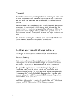


![1 Introduction
We use to think of our eyes mainly as input-organs, organs that observe the
surroundings. This is also their most important role, but in fact they also
operate as output-organs. The output they are producing is the direction in
which we are looking, thus indicating what is being focused upon. As Argyle
writes in “Bodily communication” [1], “Gaze, or looking, is of central
importance in social behavior”.
In collaborative virtual meeting-places the participants are being represented
by graphical objects, so called avatars. Figure 1.1 shows three views of the
same virtual meeting situation, three avatars sitting around a desk. One
problem with the avatars of today is that they don’t conduct facial
expressions nor show the other participants where the person who is
represented has his/her focus. It’s easy to understand that problems
concerning who addresses whom easily occur in a multi participant meeting.
To solve the problem with who is addressing whom, the avatar should face
the same object/avatar as his/her owner (the participant represented by the
avatar) focuses upon at the screen. Making the avatar pan or tilt its head is
easy, it is acquiring the information to make it act correctly that is the main
problem.
Figure 1.1 shows three snapshots from a virtual meeting situation where the
problem with visual focus has been solved by using the system described in
this report. The avatar sitting unaccompanied addresses the avatar sitting to
the left of “him” by just looking at his avatar on the screen, left avatar, upper
left image.
5](https://image.slidesharecdn.com/eb80fcef-5cc3-4ad7-bda5-cdd2a1167df0-161108214922/85/exjobb-Telia-6-320.jpg)
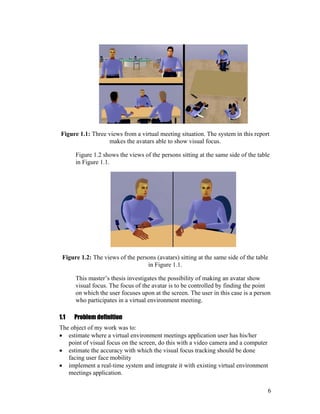
![1.2 Related work
In this section some related work that has been studied will be presented.
In the paper [2] by Roel Vertegaal et al. they discuss why, in designing
mediated systems, focus should first be placed on non-verbal cues, which are
less redundantly coded in speech than those normally conveyed by video.
This paper is related to [3].
Roel Vertgaal et al. [3] have developed a system where a commercial eye
gaze tracker was used for bringing the point of visual focus into the virtual
environment. The goal was mainly to organize different aspects of awareness
into an analytic framework and to bring those aspects of awareness into a
virtual meeting room.
To find appropriate eye gaze tracking techniques a large number of articles
were studied among them “Eye Controlled Media: Present and future State”
[4] by Arne John Glenstrup and Theo Engell-Nielsen where most techniques
are mentioned. The report [4] has an information psychology based approach.
When the appropriate techniques were found, my task was divided into two
parts, finding the facial details and processing the extracted data to find point
of visual focus. Articles studied to implement the facial detail extraction part.
Gaze Tracking for Multimodal Human-Computer Interaction [5] by Rainer
Stiefelhagen uses color information to find the face and intensities to find the
details.
Jie Yang and Alex Waibel uses a stochastical model (skin-color) for tracking
faces described in [6].
Kin Chong Yow and Roberto Cipolla describe in [7] how faces can be
located through finding facial features. The method uses a family of Gaussian
derivative filters to search and extract the features.
S.Gong et al. describe in [8] how faces can be found through fitting an ellipse
to temporal changes. A Kalman filter is applied to model the dynamics of the
ellipse parameters.
James L. Crowley and Francois Berard describe in [9] how faces can be
detected “from blinking” and from color information.
Saad Ahmed Sirohey shows in [10] that faces can be detected by fitting an
ellipse to the image edge map.
In [11] Jörgen Björkner has implemented a number of methods to detect the
face. The facial details are found using either gray levels or eye blinks.
7](https://image.slidesharecdn.com/eb80fcef-5cc3-4ad7-bda5-cdd2a1167df0-161108214922/85/exjobb-Telia-8-320.jpg)
![Martin Hunke and Alex Waibel combine color information with movement
and an artificial neural network to detect faces in [12].
Carlos Morimoto et al. uses the “bright eye effect” known from taking
pictures using a flash to locate eyes and faces. This is described in [13].
Articles studied to implement the data processing part:
Shumeet Baluja and Dean Pomerleau show in [14] that the point of visual
focus can be estimated non-intrusively by an artificial neural network. The
same thing is done by Rainer Stiefelhagen, Jie Yand and Alex Waibel in [15]
and Alex Christian Varchim, Robert Rae and Helge Ritter in [16].
1.3 How to read this report
The aim of this section is to make the report easier to read and to make the
reader read only the parts interesting for him/her.
The report is divided into five main parts
1. Basics (Chapter 2)
2. System overview (Chapter 3)
3. Details about the implementation (Chapter 4 - 7, 9)
4. Implementation justifications (Chapter 8)
5. Results, conclusions and future improvements (Chapter 10 - 12)
Part 1, Basics consists of useful fundamental information within the
concerned area. This is a part that should be briefly read if not well known to
the reader.
Part 2, System overview shows the overall relationship among all the
elements described in this report, useful to read and understand before going
any further. Readers who are interested in image processing parts only can
skip this part.
Part 3, details about the implementation describes the implementation in a
way that the system components can be re-created by the reader. It is not
necessary to read this part to understand the concept of the system.
Part 4, implementation justifications informs about why the system is built
the way it’s built and why the different selections of methods and algorithms
8](https://image.slidesharecdn.com/eb80fcef-5cc3-4ad7-bda5-cdd2a1167df0-161108214922/85/exjobb-Telia-9-320.jpg)


![2.2 Definitions
In this section some definitions are stated, these are useful be familiar with
when reading this report.
Point of visual focus: The point on which the subject’s eyes are turned
toward (not necessarily making attention to).
Avatar: [17]”A graphical icon that represents a real person in a cyberspace
system”. [18] ”In the Hindu religion, an avatar is an incarnation of a deity;
hence, an embodiment or manifestation of an idea or greater reality.”
Virtual environment: A computer generated location with non-real spatial
presence.
Detecting: Finding an object without knowing its past concerning size and
location.
Tracking: The opposite of detecting, finding an object knowing something
about where it was before.
2.3 Chromatic colors
Chromatic colors are used in this work for detecting and tracking the face.
It has been recognized that although skin-color appears to vary over a wide
range, the difference is not so much in color as in brightness. The color
distribution of the skin-color is therefore clustered in a small area of the
chromatic color space.
If R,G and B are the red, green and blue color components of an image
segment, chromatic colors will be defined by the normalization shown in
Definition 2.1.
BGR
B
b
BGR
G
g
BGR
R
r
++
=
++
=
++
=
Definition 2.1: The definition of chromatic colors.
Since r + g + b = 1, b is redundant.
11](https://image.slidesharecdn.com/eb80fcef-5cc3-4ad7-bda5-cdd2a1167df0-161108214922/85/exjobb-Telia-12-320.jpg)
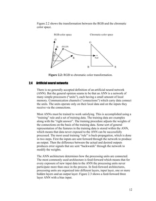


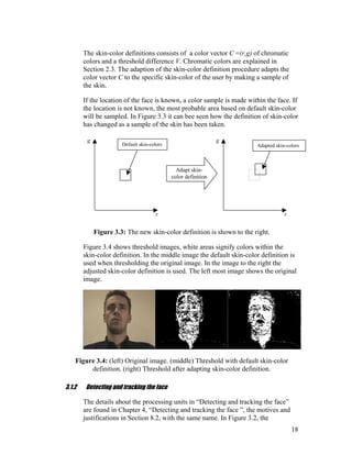


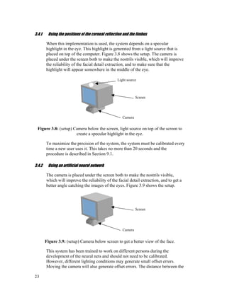

![4 Detecting and tracking the face
In Chapter 3 the system overview was described, in this chapter, the details
concerning the “Detecting and tracking the face” part will be described. See
Figure 3.2 for facial extraction overview. In Chapter 8 the approaches used
will be discussed and justified.
4.1 Adapting the skin-color definition
This procedure makes a chromatic color sample of the specific subject.
Depending on the current state, if the positions of the face details are known
or not, different methods are used. These are described in the following
sections. The methods used are discussed and justified in Section 8.2.1.
4.1.1 Facial details not known
The average chromatic colors over a segment of a row that has a default skin-
color density above a certain value will define the new skin-color mean
value.
To find the longest segment of a row that has a skin-color density above a
threshold, an integration procedure has been used. If c(x,y) is the chromatic
color-vector (r,g) in the image point (x,y) and the default skin-color Cd equals
(Rd,Gd) then I is defined:
2,22,31
)0],[),((0
)0],[),((2),,1(
])[),((1),,1(
),,(
===
≤±∉
>±∉−−
±∈+−
=
VCC
IVCyxc
IVCyxcCIyxI
VCyxcCIyxI
IyxI
d
d
d
Definition 4.1: Definition of the integration function, note that it is implicit.
Where V is the difference between default skin-color and actual pixel color
accepted to count the specific pixel as a skin-color pixel.
The function I is then used in a scanning procedure, scanning the image. To
make the algorithm a little faster the scanning steps Xscan and Yscan are set to
three and five respectively. The size of the image is Sw*Sh. The positions
(x,y)beginning and (x,y)end of the beginning and the end points of the longest
skin-colored row segment can be written as:
25](https://image.slidesharecdn.com/eb80fcef-5cc3-4ad7-bda5-cdd2a1167df0-161108214922/85/exjobb-Telia-26-320.jpg)
![endendbeginning
hscan
SXx
end
yxIyxIxx
SYyIyxIyx
wscan
∈∀=⇐⇐
∈∀⇐
=
0),,()max(
]::0[)],,([max),(
::0
(4.1-1)
Figure 4.1 shows the procedure graphically over a segment of a row.
Figure 4.1: Integration procedure graphically.
The color sample Csample is simply an average made over this segment:
∑=−
=
end
beginning
x
xx
end
beginningend
sample yxc
xx
C ),(
1
(4.1-2)
The right image in Figure 4.2 shows a threshold image after the skin-color
adaptation procedure. In the middle threshold image the default skin-color
definition is used.
Figure 4.2: (left) original image. (middle) Threshold image, default skin-color
definition. (right) Threshold image, adapted skin-color definition.
26](https://image.slidesharecdn.com/eb80fcef-5cc3-4ad7-bda5-cdd2a1167df0-161108214922/85/exjobb-Telia-27-320.jpg)
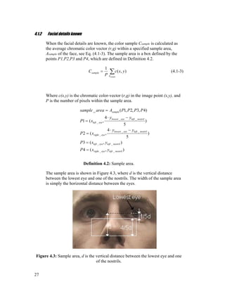
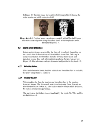
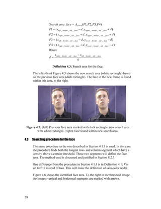


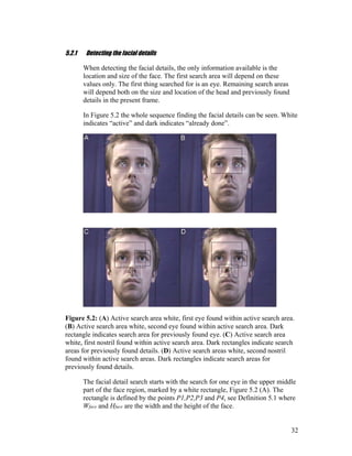


![5.3 Searching procedure for the facial details
In this section the algorithm used for finding the facial details will be
described. For an overview, see Figure 3.2. The procedure is discussed and
justified in Section 8.3.3. The details will be searched within the areas
defined in Section 5.2.
Each eye is located through finding the “grayest” pixel within the specific
search area. The “grayest” pixel in this case is the pixel with the least
difference in red, green and blue intensity, see Section5.1.
If c(x,y) is the color-vector (r,g,b) in the image point (x,y) and the search area
is Asearch, the position of the eye (x,y)eye is given by:
[[
]]
3
),(),(),(
),(
),(),(
,),(),(
,),(),(maxmin),(
),(
yxcyxcyxc
yxc
where
yxcyxc
yxcyxc
yxcyxcyx
bluegreenred
av
avblue
avgreen
avred
Ayx
eye
search
++
=
−
−
−⇐
∈
(5.3-1)
The nostrils are located through finding the best template match. The
template is shown to the right in Figure 5.5.
If c(x,y) is the color-vector (r,g,b) in the image point (x,y) and the search area
is Asearch, the position of the nostril (x,y)nostril is defined by:
±±+∆±∆±+⋅
⇐
∑∑=∆
∈
)3,3(),(3),(10
min),(
2,1
),(
yxcxyyxyxcyxc
yx
red
xy
redred
Ayx
nostril
search
(5.3-2)
Figure 5.5 shows the template both in the image (left side), and with the
weights (right side).
37](https://image.slidesharecdn.com/eb80fcef-5cc3-4ad7-bda5-cdd2a1167df0-161108214922/85/exjobb-Telia-38-320.jpg)


![[ ][ ]
±±⋅−−⇐ ∑
==
==
3',3'
0',0'
)','()]'4(),'4min[(min),(
yx
yx
blue
A
pupil yyxxcyxyx
search
(5.5-1)
Figure 5.7 shows the procedure graphically, the outer square is the search
area and the inner is the area corresponding to the pyramid.
Figure 5.7: Graphical illustration of searching procedure, the pyramid function
sweeps over the eye area to find the center of the pupil. Outer dark square is the
search area, the inner square corresponds to the pyramid function.
40](https://image.slidesharecdn.com/eb80fcef-5cc3-4ad7-bda5-cdd2a1167df0-161108214922/85/exjobb-Telia-41-320.jpg)

![Finding the specular
highlight
Enlarging the area
around the highlight
Histogram
equalization
Improving the
highlight position
and finding the
limbus on both
sides of highlight
Estimate point of
visual focus from
the position of the
highlight relatively
the limbus
Preprocessingtheeye
images
Estimatingthepoint
ofvisualfocus
Increasing contrast
Findingthe
specualr
highlight
Figure 6.1: A graphical overview of the process and of the content of this section.
Dashed boxes indicate sub sections. To the right the outcome of each step is shown.
6.1.1 Finding the specular highlight
The eyes are searched for the specular highlight. It’s located through
searching for a bright area surrounded by a dark one in the neighborhood of
the center of the pupil.
If c(x,y) is the color-vector (r,g,b) in the image point (x,y) and the search area
is Asearch, the position of the highlight (x,y)highlight is given by:
[ ])','(),(15max),(
3';3'
),(
∑ ±=±=
∈∀
−⋅=
yyxx
redred
Ayx
Highlight yxcyxcyx
search
(6.1-1)
The search Asearch, is defined in Definition 6.1.
42](https://image.slidesharecdn.com/eb80fcef-5cc3-4ad7-bda5-cdd2a1167df0-161108214922/85/exjobb-Telia-43-320.jpg)


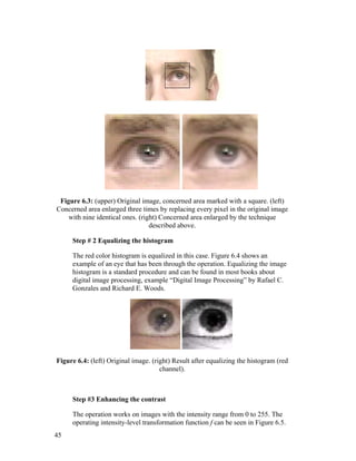

![6.1.3 Estimating the point of visual focus
To estimate the point of visual focus, the positions of the specular highlight
and two limbus points at the side of the highlight must be found. The
specular highlight is re-located within a small area around the previous
location. The highlight is found by matching a template.
If c(x,y) is the color-vector (r,g,b) in the image point (x,y) and the search area
is Asearch, the position of the highlight (x,y)highlight is given by:
[ ])',(
'
4
),'(
'
4
),(4
max),(
4,2'4,2'
),(
yxc
y
yxc
x
yxc
yx
red
yyyxxx
redred
Ayx
highlight
search
⋅+⋅+⋅
=
∑∑ ±±=±±=
∈∀
(6.1-2)
If the position of the first found highlight, Section 6.1.2, is (x,y)old_highlight, the
search area is defined by:
20
)(
3),(
__
_
eyelefteyeright
highlightoldsearch
xx
yxA
−
⋅±=
Definition 6.3: The definition of the search area for the re-location of the specular
highlight.
Figure 6.7 shows template on top of the highlight region.
Figure 6.7: The template used for re-locating the specular highlight placed on a
fragment of the eye.
47](https://image.slidesharecdn.com/eb80fcef-5cc3-4ad7-bda5-cdd2a1167df0-161108214922/85/exjobb-Telia-48-320.jpg)
![Having found the highlight, searching the limbus is done by looking
sideways for the largest gradient.
If c(x,y) is the color-vector (r,g,b) in the image point (x,y) and the search
areas are Asearch1 and Asearch2, the positions of the limbus points (x,y)limbus are
given by:
[ ]
[ ]),2(),1(),2(),1(max
),(
),2(),1(),2(),1(max
),(
2
1
),(
_
),(
_
yxcyxcyxcyxc
yx
yxcyxcyxcyxc
yx
redredredred
Ayx
imbuslright
redredredred
Ayx
imbuslleft
search
search
−−−−+++=
+−+−−+−=
∈∀
∈∀
(6.1-3)
Where the search area Asearch1 is defined by:
3
6
)2,7(4
)2,(3
)2,7(2
)2,(1
)4,3,2,1(
__
1
⋅
−
=
−−=
−−=
+−=
+−=
=
eyelefteyeright
highlighthighlight
highlighthighlight
highlighthighlight
highlighthighlight
search
xx
d
where
yxP
ydxP
yxP
ydxP
PPPPAbusmlileftareaSearch
Definition 6.4: The point defining the search area for the left limbus point.
Search area Asearch2 is Asearch1 flipped horizontally around the specular
highlight.
In Figure 6.8 the positions of the specular highlight and the two limbus points
are marked with crosses.
Figure 6.8: Specular highlight and limbus points found, marked with crosses.
To find the actual point of visual focus the system must be calibrated, see
Section 9.1. If c and d are defined as shown in Figure 6.9 and Rx is the
horizontal resolution of the screen, the point of visual focus X is calculated
as:
48](https://image.slidesharecdn.com/eb80fcef-5cc3-4ad7-bda5-cdd2a1167df0-161108214922/85/exjobb-Telia-49-320.jpg)
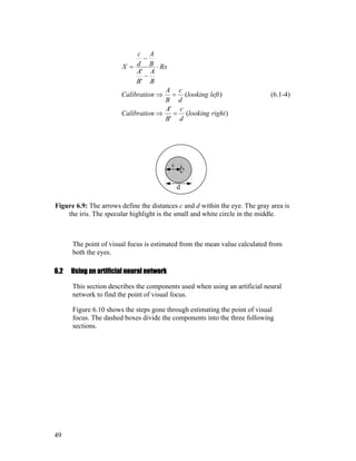
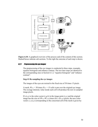

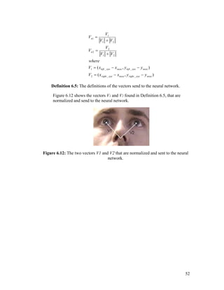

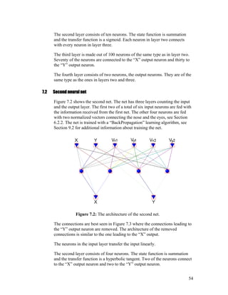


![Research groups [15], [14] and [16] have shown that it is possible to
construct eye gaze tracking systems that meet with the requirements, they are
non-intrusive, but still allows the user to move. The precision in these
systems is not as good as for some of the ones on the market, but they still
seem to meet the requirements set for this system. These systems are based
on wide-angle video images and neural networks.
The requirements, problem definition and the experience of others lead to
solutions based on wide-angle video images. The first approach implemented
was chosen since it’s what’s considered being traditional eye gaze tracking,
this implementation however is non-intrusive since it uses video images,
which is not traditional. The artificial neural network approach was chosen
because the success among others.
8.2 Detecting and tracking the face
This section contains justifications concerning the choices of components
used for detecting and tracking the face, see Section 3.1 for an overview and
Chapter 4 for the implementation details.
There are a number of ways to detect faces in images. The task of this thesis
was not however to develop another face tracker. Going through existing
face-tracking techniques one discovers that many of them take a lot of CPU
power. The CPU power is limited since this system will run simultaneously
with the virtual environment meetings application. To keep the number of
computer calculations at an acceptable level, one should try to find face
features at the lowest possible level. The smallest piece of information that
can classify faces in images is probably the color of one single pixel. The
decision to use image color information to extract the face is based on the
fact mentioned above.
Using color information when tracking the face is often combined with
motion estimation. In this system this is not implemented, the user of the
system is a participant in a virtual meeting and is not thought of as being
moving around a lot.
In Section 1.2 articles are presented that were studied to choose a face
tracking technique.
8.2.1 Adapting the skin-color definition
The decision to use color information extracting the face leads to the need of
a skin-color representation. The representation used is based on chromatic
colors described in Section 2.3. Although the difference in human skin-color
is small in the chromatic color-space, it’s safer to look for the specific skin-
59](https://image.slidesharecdn.com/eb80fcef-5cc3-4ad7-bda5-cdd2a1167df0-161108214922/85/exjobb-Telia-60-320.jpg)


![8.2.3 Search procedure
There are several possible ways to find the face within the search area. The
most common way of finding large areas from categorized pixels is labeling
of connected components described by Rafael C. Gonzalez and Richard E.
Woods in [19]. This will however cast a lot of work on the computer and still
not guarantee that the entire face will be found since it is not sure that the
face can be found in one piece. Better is finding some sort of value of the
skin-color density.
The method used in this implementation is a very computer computational
cheap way of finding an area with a high a density of skin-colored pixels.
The method was developed to cast as little work as possible on the computer
but still to be working properly.
The skin-color density threshold is set by the constants C1 and C2 in
Definition 4.1. With the selections of C1 = 3 and C2 = 2, areas with a skin-
color density of 2/5 (skin-color pixels) per (pixel) and above will produce
skin-color segments. The decision to use the density threshold 2/5 was based
on studies of different threshold images such as the image in Figure 8.4.
Figure 8.4: An example of an image used for deciding the “density” threshold that
is used when detecting and tracking the face.
8.3 Detecting and tracking the eyes and nostrils
This section contains justifications concerning the choices of components
used for detecting and tracking the eyes and nostrils, see Section 3.1.3 for an
overview and Chapter 5 for the implementation details.
What to look for, and where to look when looking for the eyes and nostrils
are the main issues of this section
63](https://image.slidesharecdn.com/eb80fcef-5cc3-4ad7-bda5-cdd2a1167df0-161108214922/85/exjobb-Telia-64-320.jpg)
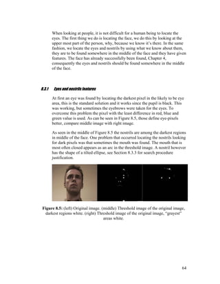
![In Table 8.2 some eyes and nostrils features are listed. The ones used in this
system are marked with a star (*), the sections in which they are used in the
implementation are indicated.
Summarizing the eyes and nostrils features.
Eye features:
1. The pupil is black * (Section 5.5)
2. The sclera is white
3. Low difference in R,G,B values * (Section 5.3)
4. The iris and pupil are circular
5. An eye sometimes blinks
6. The surface of the eye reflects light * (Section 6.1.1)
7. The Retina reflects light
Nostril features:
1. Dark * (Section 5.3)
2. Has the shape of a tilted ellipse * (Section 5.3)
Table 8.2: Some eye and nostril features, the ones used in this system are marked
with stars (*).
8.3.2 Search areas
When detecting the facial details, the only information available is the
location and size of the face. The start search area is chosen to maximize the
probability of finding at least one eye in it. It is also chosen to minimize the
probability of finding any distracting items such as dark hair, the mouth or
the ears. The nostrils are not a big threat since they are not “gray”, see Figure
8.5. Ones one eye has been found the rest of the search areas will come
naturally.
When tracking the facial details no information about the face location and
size is used, the details are more precise and will better define the new search
areas. The size of the areas to search for the new details is chosen on the
basis of the theory in Section 8.2.2
8.3.3 Search procedure
Humans have a great ability to recognize visual patterns [20], computers
however are not very good at this since they can’t handle more than one
piece of information at the same time. The fastest way to find something with
a computer is therefore to find a specific feature at pixel level, distinguishing
the thing looked for and then look for pixels with this feature. Sometimes this
is however not enough, then the shape of the thing looked for can help.
65](https://image.slidesharecdn.com/eb80fcef-5cc3-4ad7-bda5-cdd2a1167df0-161108214922/85/exjobb-Telia-66-320.jpg)


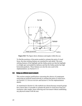
![8.5.1 Preprocessing the eye images
To make the ANN learning process as easy as possible, the images of the
eyes are processed in a way that makes different colored eyes look uniform.
The size in pixels of the interesting parts of the eyes will depend on the size
of the subject in the image, in other words how far from the camera the user
is situated and the zoom factor of the camera. Since the number of input
neurons is fix this means that if the same eye areas are to be sent to the
network, the images of the eyes must be resized to a fix size. Since the user
most often is situated relatively close to the screen and the therefor close to
the camera, the function resizing the eye images almost always will decrease
the size of the eye images to the fixed size. This means that there is no need
for an advanced resizing algorithm that can enlarge images.
Different lighting conditions may affect the temperature of the images, to
normalize the color distribution the, histograms of the eye images are
equalized. This will also enhance the contrast in the images. In the ANN
architecture used in this system, this step is very important since the network
not is used as a classifier, for more information, see Section 8.6.
The image contrast is enhanced even more to reduce the amount of
distracting information, which makes the images more uniform.
8.6 ANN implementation
This section justifies the architecture of the artificial neural network used in
the second implementation, see Figure 3.1 for an overview. In Chapter 7 a
description of the architecture can be found. How to achieve and how to
preprocess input data is found in Section 6.2. Collecting training data is
described in Section 9.2.
8.6.1 Discussion
Choosing the architecture is crucial for the result in many ways.
Theoretically three layers are sufficient for solving any problem that can be
solved using four and more layers. This does not mean that all problems
solvable by neural nets should be solved by a three layer net, some four (or
more) layer nets is much easier to train solving the same problem. Optical
character recognition is a problem often solved by neural nets containing
more than one hidden layer. Le Cun et al. [21] used a six-layer configuration
solving the optical character recognition problem.
A large number of architectures have been tried in this project including the
ones used by Rainer Stiefelhagen, Jie Yang and Alex Waible [15] and
Shumet Maluja and Dean Pomerleau [14]. The systems made by the persons
70](https://image.slidesharecdn.com/eb80fcef-5cc3-4ad7-bda5-cdd2a1167df0-161108214922/85/exjobb-Telia-71-320.jpg)
![mentioned above used a configuration that generates a gaussian output over a
number of output neurons. This configuration was also implemented, but
generated a number of connections and never worked as well as the ones
implemented by the two research groups. The first and corresponding net in
this system, seen in Figure 7.1 has 10312 connections counting the bias. The
nets used by Rainer Stiefelhagen, Jie Yang and Alex Waible [15] generate at
least 20140 connections even though only 400 input neurons were used. The
number of connections is proportional to the amount of computer work,
which means twice as much work for the computer using the nets used by
Rainer Stiefelhagen et al.
As mentioned earlier, the system implemented uses two neural nets. The first
one estimates the orientation of the eyeball in relation to the eye socket and
the second one is making the system invariant to head pans and tilts. A
disadvantage that comes with the architecture of the first net is that it’s
sensitive to “image temperature“, in other words the total sum of the
intensities in the image. This problem causes an offset error. Theoretically
this problem would disappear if the eye images histograms could be
equalized perfectly, this is however not the case since the color depth is
limited. This offset problem is due to the architecture, the net works as a
function approximater and not as a classifier. The nets used by the research
groups do not have this problem since they use their nets to classify the eye
images into eyes looking at different segments of the screen.
Another issue is how much information to put into the neural net and if
features should be added. Shumet Maluja and Dean Pomerleau [14] used a
light source to create a specular highlight in the eye and one image of the eye
that was 40x15 pixels. The light source introduced, adds information about
the relation to the surroundings as can be seen in Section 6.1.
The larger the eye images sent to the neural net are, the higher is the camera
resolution needed, unless the eyes are zoomed. But zooming the eyes will set
constraints on user movement. The camera image used in this system has a
resolution of 352x288, Figure 8.9 shows the size of an area with 30x15
pixels, this area is the interesting area to process with a neural net.
71](https://image.slidesharecdn.com/eb80fcef-5cc3-4ad7-bda5-cdd2a1167df0-161108214922/85/exjobb-Telia-72-320.jpg)


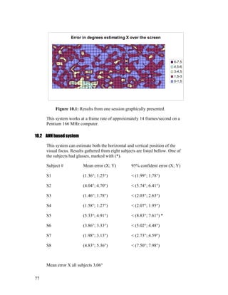


![12 Future improvements
Because of the limited time, the systems are not ideal and could still use
some changes. This chapter contains some ideas that could make the systems
both more reliable and precise in the estimation.
12.1 Extracting facial details
Below some ideas to improve reliability and precision when extracting the
facial details are listed.
Using color templates and a dynamic background extraction could enhance
tracking [22].
If the head motion is estimated, the search areas could be reduced, hence
enhancing the reliability of tracking.
The skin-color adaptation could use a more detailed definition, color variance
could also be sampled.
The geometric relation check could use an individual three-dimensional
representation.
The pupil center positioning could be performed by an ANN fed with re-
scaled images (to a fix size) of the eyes. The ANN could even decide if the
eyes really are eyes, if the method finding the eyes is not reliable.
12.2 Processing extracted data to find point of visual focus
If extracting facial details works properly, this part often works acceptable.
To improve the systems there are however some things that can be done.
12.2.1 Corneal reflection based system
To avoid the uncomfortable light source, infrared light could be used. Then
the “bright-eye-effect” could be used as well. This makes the technique
almost similar to the one described in APPENDIX A (6). The difference
would be that low-resolution images are used instead of high-resolution
images. Using low-resolution images makes positioning of small details
harder; the pupil can still be positioned quite well using sub pixel
classification. To increase the accuracy of the reflection, many reflections
82](https://image.slidesharecdn.com/eb80fcef-5cc3-4ad7-bda5-cdd2a1167df0-161108214922/85/exjobb-Telia-83-320.jpg)
![could be generated; finding all these reflections would improve the position
of every one of them if the relative positions of the light sources were known.
The idea of using more than one light source were tested briefly.
Experiments with light sources in different colors were conducted. The
specular highlights generated from the different light sources were however
hard to recognize as different in color, probably due to the camera used in the
experiments. Using multiple white light sources would work, but the total
amount of light reaching the eyes would be very distracting.
The positioning of the limbus could be improved by approximating arcs. This
would cast some work on the CPU, but since this implementation uses very
few calculations maybe it wouldn’t matter.
12.2.2 ANN based system
To make this system more reliable and general (to make it work on
everyone), more subjects should be used collecting the training data for the
nets. This would make the ANN eye socket shape invariant. Different
lighting conditions during the sessions would also make the system better.
The preprocessing of the eye images could be improved, the idea is to make
the eyes uniform (make all eyes look the same). A better contrast function
could be used together with an edge enhancer. Still the shape of the eye will
remain, the influence of this factor can be reduced by data collection, see
above.
Another way of making the ANN invariant to eye socket shapes, could be to
subtract a template of the individual’s eye from the eye image processed. The
template should then be taken in advance as a part of the calibration.
As discussed in Section 8.6.1 the network architecture in this implementation
is sensitive to image temperature. To eliminate this problem the total sum of
the intensities could be sent along with the images of the eyes to the ANN.
Additional features could be added to the eye images by adding infrared light
sources. These light sources would be reflected at the cornea and hence add
information about the relation of the eye orientation relative the surrounding.
Another thing worth trying is using a gaussian output representation as done
in [14],[15] and [16], but instead of using a number of X and Y output
neurons, the screen should be segmented into a number of (x,y) positions.
83](https://image.slidesharecdn.com/eb80fcef-5cc3-4ad7-bda5-cdd2a1167df0-161108214922/85/exjobb-Telia-84-320.jpg)
![References
[1] Argyle.M 1988, “Bodily communication” 2 ed. ISBN 0-415-051142,
Routledge, page 153.
[2] Roel Vertegaal, Harro Vons and Robert Slagter, “The Gaze Groupware
System: Joint Attention in Mediated Communication and Collaboration”
(http://reddwarf.wmw.utwente.nl/pub/www/…tegaal/publications/GAZE/gaz
epaper.htm
[3] Roel Vertegaal, Boris Velichkovsky and Gerrit van der Veer, “Catching
the Eye: Management of Joint Attention in Cooperative Work” SIGCHI
Bulletin (29)4, 1997.
(http://reddwarf.wmw.utwente.nl/pub/persons/vertegaal/publications/s…/catc
h.htm)
[4] Thesis: Arne John Glenstrup and Theo Engell-Nielsen “Eye Controlled
Media: Present and future State” University of Copenhagen 1st
June 1995
[5] Diplomarbeit: Rainer Stiefelhagen “Gaze Tracking for Multimodal
Human-Computer Interaction” Institut für Logik, Komplexität und
Deduktionssysteme, Karlsruhe. September 12, 1996.
[6] Jie Yang and Alex Waibel “Tracking Human Faces in Real-Time” CMU-
CS-95-210. November 1995
[7] Technical report: Kin Choong Yow and Roberto Cipolla “Towards an
Automatic Human Face Localization System” Department of Engineering,
University of Cambridge.
[8] S.Gong, A.Psarrou, I.Katsoulis and P.Palavouziz “Tracking and
Recognition of Face Sequences” Department of Computer Science, Univerity
of London and School of Computer Science, University of Westminster
[9] James L. Crowley and Francois Berard, “Multi-Modal Tracking of Faces
for Video Communications” GRAVIR – IMAG, I.N.P. Grenoble.
[10] Thesis: Saad Ahmed Sirohey “HUMAN FACE SEGMENTATION
AND IDENTIFICATION”, CAR-TR-695, CS-TR-3176, DACA 76-92-C-
0009
[11] Thesis: Jörgen Björkner “Face detection and pose estimation” TRITA-
NA-E9760, KTH Stockholm.
84](https://image.slidesharecdn.com/eb80fcef-5cc3-4ad7-bda5-cdd2a1167df0-161108214922/85/exjobb-Telia-85-320.jpg)
![[12] Martin Hunke and Alex Waibel, “Face Locating and tracking for
Human-Computer Interaction” School of Computer Science, Carnegie
Mellon University.
[13] Carlos Morimoto, Dave Koons, Arnon Amir and Myron Flickner. “Real-
Time Detection of Eyes And Faces” IBM Almaden Research Center.
[14] Shumeet Baluja and Dean Pomerleau “Non-Intrusive Gaze tracking
Using Artificial Neural Networks” CMU-CS-94-102 School of Computer
Science, Carnegie Mellon University.
[15] Rainer Stiefelhagen, Jie Yand and Alex Waibel “Tracking Eyes and
Monitoring Eye Gaze” Interactive Systems Laboratories, University of
Karlsruhe, Carnegie Mellon University.
[16] Alex Christian Varchim, Robert Rae and Helge Ritter section “Image
Based Recognition of Gaze Direction Using Adaptive Methods” in “Lecture
Notes in Artificial Intelligence 1371, Gesture and Sign Language in Human-
Computer Interaction” Ipke Wachsmuth and Martin Fröhlich, Springer
[17] Webopedia: http://webopedia.internet.com/TERM/a/avatar.html,
December 1998.
[18] http://whatis.com/avatar.htm, December 1998.
[19] Rafael C. Gonzalez and Richard E. Woods “Digital Image Processing”
ISBN 0-201-60078-1, page 173.
[20] Cognitive Psychology and its Implications, John R. Anderson, WH
Freeman company
[21] Y. Le Cun, B. Boser, J.S. Denker, D. Henderson, R.E. Howard, W.
Hubbard, and L. D. Jackel, “Handwritten Digit Recognition with a Back-
Propagation Network” AT&T Bell Laboratories, Holmdel, N.J. 07733.
[22] Simon A. Brock-Gunn, Geoff R. Dowling and Tim J. Ellis “Tracking
using colour information” Department of Computer Science, City University
London.
85](https://image.slidesharecdn.com/eb80fcef-5cc3-4ad7-bda5-cdd2a1167df0-161108214922/85/exjobb-Telia-86-320.jpg)