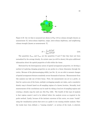
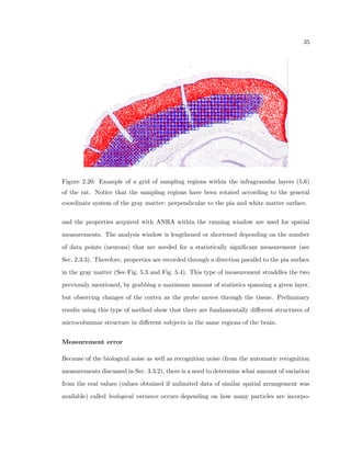
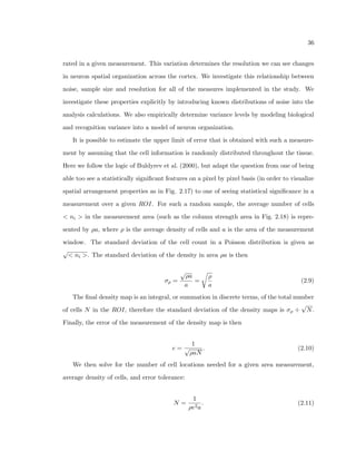
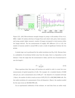
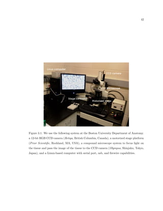
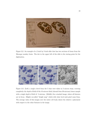
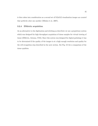
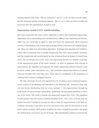
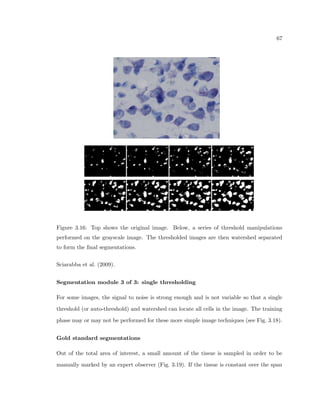
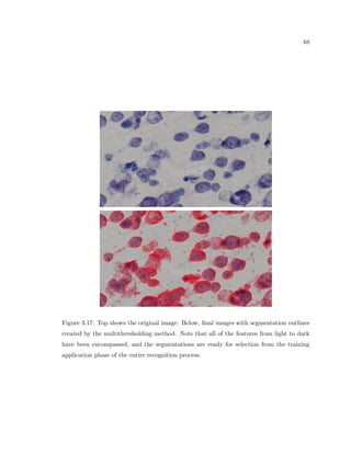
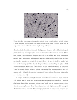
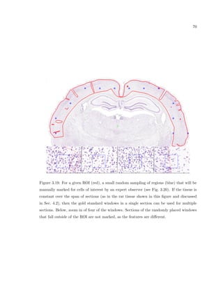
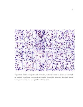
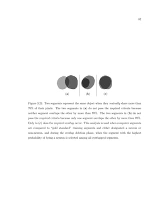
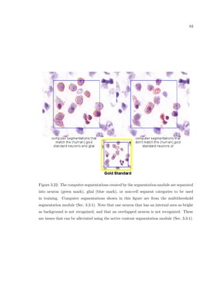
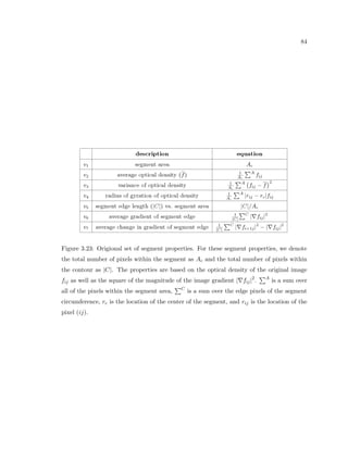
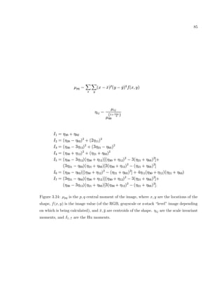
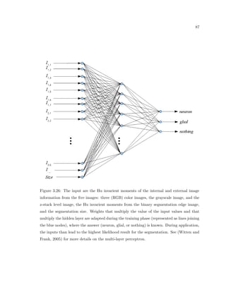
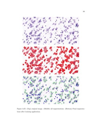
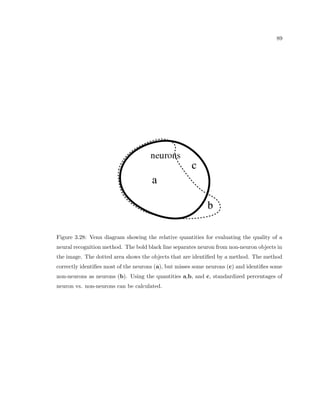
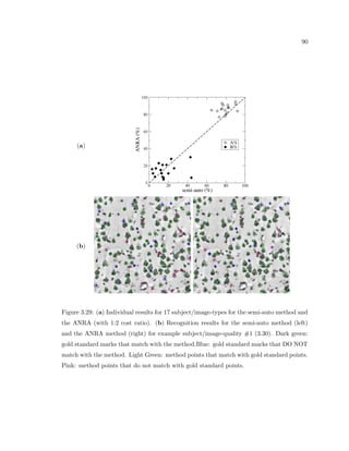
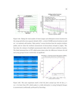
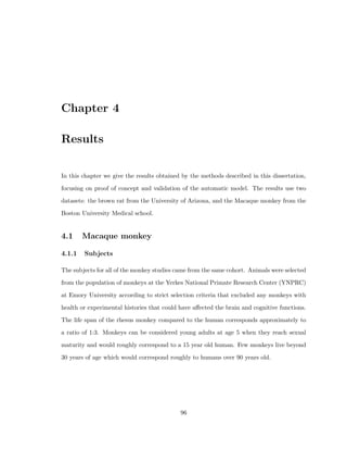
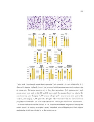
Download to read offline


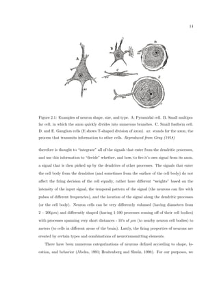
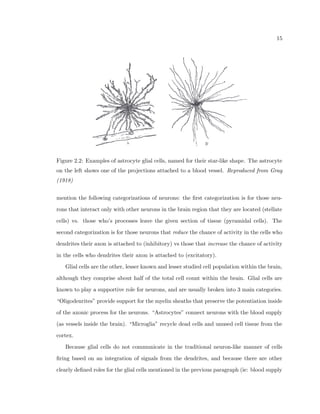
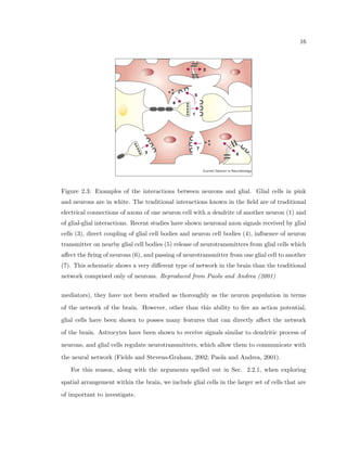
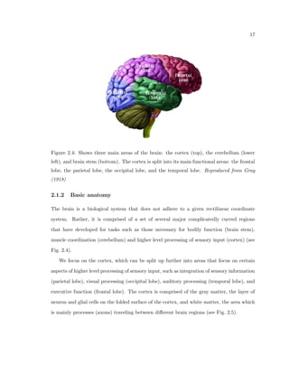


This dissertation examines methods for measuring the spatial arrangement of neurons and glial cells in the mammalian cortex. The document begins with an introduction discussing the importance of studying brain cell arrangement and the need for quantitative tools. It then provides a literature review on brain anatomy, spatial arrangement mechanisms, and existing measurement theories. The experimental method section describes a three-part process: 1) digitizing tissue samples at high resolution, 2) developing algorithms to recognize cells in the digitized images, and 3) analyzing the data using metrics like cell counts, density maps, and cross-correlations. Results are presented on tissue samples from the macaque monkey and rat brain, focusing on specific cortical areas. Future studies are proposed to integrate the data, analyze


