Download to read offline


![to extract the foreground. Often these methods take little use of temporal re-
dundancy, and are slow because of the large amount of computations needed.
The second approach is dierent, often using pixel by pixel computations and
only a few computations per pixel. In general the latter methods are fast
and may be implemented in real-time applications. The drawback of these
methods is that they are, due to the lack of complexity in the algorithms,
sensitive to noise and often need a static environment to be able to function.
1.2 Related work
There are a few simple algorithms for tracking, for example: detection of
discontinuities using Laplacian and Gaussian lters, often implemented with
a simple kernel [1]; thresholding; and motion detection with reference image.
These algorithms are simple, but sensitive to noise, and hard to generalize. A
set of more advanced algorithms involves iterations and/or transformations,
such as the Hough transform, region based segmentation and morphological
segmentation. These algorithms are generally more stable concerning noise,
although as pictures and/or frames grows larger, these algorithms get slow [1].
Other algorithms make use of pattern recognition, such as neural net-
works, maximum-likelihood and support vector machines [2]. First the image
has to be translated into something that the pattern recognition algorithms
understand. The image is processed to a so-called feature vector. The ma-
jority of pattern recognition algorithms require a set of training data to form
the decision boundary. The training is often slow, however thereafter the
algorithm is fast. The problem is that extracting the feature vector might
2](https://image.slidesharecdn.com/sonaproject-111012233839-phpapp02/85/Sona-project-8-320.jpg)
![be a demanding task for the computer.
There is a number of interesting approaches to object tracking. In the
study by Kyrki et al [3] they use both model-based features such as a wire
frame combined with model-free features such as points of interest on a calcu-
lated surface. In the study by Doulamis et al [4] they use an implementation
of neural networks to track objects in a video stream. The neural network
is adaptive and changes over time as the object translates. In the study by
Comaniciu et al [5] a kernel-based solution is used for identifying an object.
In a study, Amer [6] uses voting based features and motion to detect objects,
which are tuned for real time processing. In the PhD thesis by Kragi¢ [7], a
multiple cue algorithm is presented, using features that are fast to compute
and relying on the assumption that not everyone fails at the same time. In
the study by Cavallaro et al [8] a hybrid algorithm is presented using infor-
mation about both objects and regions. In the study by Gastaud et al [9]
they track objects using active contours.
Kragi¢ [7] uses multiple cues for better tracking. Instead of using multiple
cues of fast algorithms, the approach in the present thesis takes the advantage
of the fast and also the advanced algorithms in order to achieve a system that
outperforms the simple algorithms, and operates faster than the advanced
ones.
3](https://image.slidesharecdn.com/sonaproject-111012233839-phpapp02/85/Sona-project-9-320.jpg)


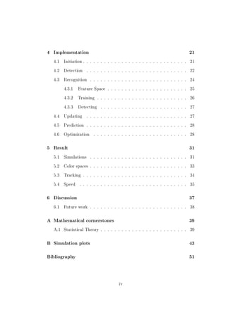
![Chapter 3
Method
3.1 Adaptive lters
An adaptive lter is a lter that changes over time depending on the signal.
For a resumé of the statistical theory used, see appendix A.1. Assume that
you have two non-stationary signals with zero mean and known stochastic
functions, hence covariance and cross-covariance
ryy (n, m) = E[y(n)y(n + m)]
rxy (n, m) = E[x(n)y(n + m)].
The problem of estimating x(n) given past y(n) may be written as
N −1
x(n) =
ˆ θ(k)y(n − k) = Y T (n)θ,
k=0
9](https://image.slidesharecdn.com/sonaproject-111012233839-phpapp02/85/Sona-project-15-320.jpg)
![where Y (n) = [y(n), ..., y(n − N + 1)] and θ = [θ(0), ...θ(N − 1)]T . The MSE
is then given by
MSE(n, θ) = E[(x(n) − x(n))2 ].
ˆ
The optimal θ may be received by the orthogonality condition which states
that Y T (n)θ is the linear MMSE of x(n) if the estimation error is orthogonal
to the observations Y (n)
E[(x(n) − Y T (n)θ)Y (n)] = 0. (3.1)
If we dene the the covariance matrices
ΣY x (n) = E[rxy (n, n), ..., rxy (n, n − N + 1)]
ΣY Y (n) = E[Y (n)Y T (n)]
ryy (0) ryy (1) . . . ryy (N − 1)
ryy (1) ryy (0) . . . ryy (N − 2)
= .
. .. .
. . .
. .
ryy (N − 1) ryy (N − 2) . . . ryy (0)
Insert this in 3.1 and we get
ΣY x (n) − ΣY Y (n)θ = 0,
from this we get θopt
θopt (n) = Σ−1 (n)ΣY x (n)
YY
10](https://image.slidesharecdn.com/sonaproject-111012233839-phpapp02/85/Sona-project-16-320.jpg)
![the gradient then is
∂
M SE(n, θ) = −2(x(n) − Y T (n)θ)Y (n) (3.5)
∂θ
if we insert 3.5 into 3.2 we get
ˆ ˆ
θ(n) = θ(n − 1) + µY (n) x(n) − Y T (n)θ(n − 1) (3.6)
The theory for this section was collected from Hjalmarsson et al [10], also
suppling more information about adaptive lters.
3.2 Motion detection
Motion detection is often built into a larger system and is tweaked to t
the other algorithms. One of the commonly used algorithms is to take a
threshold on a dierence image
1 |img(x, y, t) − img(x, y, t − 1)| T
if
d(x, y) = .
0
else
Where T is a threshold variable. Even better is to use a reference image
ref(x, y, t) = α · ref(x, y, t − 1) + (1 − α) · img(x, y, t) (3.7)
12](https://image.slidesharecdn.com/sonaproject-111012233839-phpapp02/85/Sona-project-18-320.jpg)
![and then use this reference image to take the threshold
1 |img(x, y, t) − ref(x, y, t)| T
if
d(x, y) = (3.8)
0
else
The rate of which the reference image is updated over time is controled by
α [1]. This is a fast algorithm but sensitive to noise.
Irani et al [11] has developed a method for robust tracking of motion.
In the study they use multiple scales and translations to detect and track
motions. Though this is a robust technique it puts a heavy load on the
hardware, especially at the resolutions used in the present thesis.
3.3 Pattern recognition
When you use Pattern recognition algorithms, you can seldom supply raw
data, such as a video or audio stream into the algorithms. The algorithms
will need some sort of feature(s). These features span a domain called the
feature space. The choice of feature space is essential and in some cases
even more critical than the choice of pattern recognition algorithm. This is
because you want to keep the dimensionality as low as possible, since the
higher dimensionality the more training data is needed and the algorithms
put heavier load on the computer, but if the dimensionality is too low the
ability to separate patterns is reduced. If all statistics are known in advance,
it is possible to analytically decide an optimal decision surface. However
in reality this never happens. Instead, a training set that is supposed to
represent the distribution of the signal/pattern is used to tune the chosen al-
13](https://image.slidesharecdn.com/sonaproject-111012233839-phpapp02/85/Sona-project-19-320.jpg)
![gorithm. There is a number of dierent algorithms with dierent approaches
in how to use the training set and the dierent a prioris.
3.3.1 Parametric algorithms
Parametric algorithms use the training set to train distributions chosen ear-
lier. When the distributions of the dierent patterns are trained the deci-
sion boundary can be calculated using for example maximum likelihood or
Bayesian parameter estimation. These algorithms generally have good con-
vergence and performance if they are tuned right. However quite a lot of
tuning is needed to adapt these algorithms for dierent problems. Another
problem is the curse of dimensionality, which appears when the feature space
increases in dimensionality [2]. To cope with this problem it is possible to
use Principal component analysis (PCA). PCA uses eigenvectors to decrease
the dimensionality of the feature space [2]. The strength of parametric algo-
rithms is that knowledge about the distributions can be taken into account
making better use of the training data available.
3.3.2 Nonparametric algorithms
In the previous section we discussed the idea behind algorithms that uses
training data to estimate pre-decided distributions. Unfortunately the knowl-
edge about the distribution of the patterns is rarely available. Nonparametric
algorithms do not assume any special distribution, instead they rely on the
training data to be accurately representative of the patterns.
One of the most known nonparametric algorithms is kn nearest neighbors.
14](https://image.slidesharecdn.com/sonaproject-111012233839-phpapp02/85/Sona-project-20-320.jpg)
![The algorithm uses the training data to calculate the kn nearest neighbors
to the point in the feature space corresponding to the pattern that is to be
classied. The pattern that the majority of the kn neighbors belongs to is
assumed to be the pattern connected with that point. The strength of this
algorithm is the fact that with sucient training data it is able to represent
complex distributions. The drawback is that it puts a heavy load on the
computer and the complexity increases with the dimensionality and number
of training data.
3.3.3 Linear discriminant
In the previous sections two techniques with dierent approaches on how to
use the training set given have been discussed.
This third algorithm is more or less in between the two previous algo-
rithms. We do not dene a specic distribution in advance and we do not
keep all the training data as base for calculations during run time. The
training data is used directly to train the classier which is a set of linear
discriminant functions
g(x) = wt x + w0
where x is the point in the feature space that is supposed to be classied, w
is the weight vector and w0 is the bias [1]. Depending on what problem to
solve, a number of discriminant functions can be trained and used in recog-
nition problems. For instance if the classier is supposed to be a binary, one
discriminant function is sucient. If there are many patterns that are sup-
posed to be classied, the discriminant functions can be designed in multiple
15](https://image.slidesharecdn.com/sonaproject-111012233839-phpapp02/85/Sona-project-21-320.jpg)
![data is mapped into the higher dimension the new data is processed in the
same manner as regular linear SVM. The techniques for choosing dimen-
sions and making general kernels is a eld of research out of scope for this
thesis. [12]
The linear SVM is similar to the binary linear discriminant. The main
dierence from linear discriminant function is that during training the SVM
algorithm works towards maximizing the distance from the training data
and the hyper plane, called margin maximization. This often results in a
hyper plane that produces good results also when only small training sets
are available.
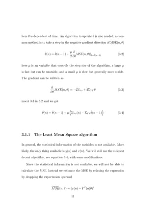
The training of the SVM is a minimization process of a cost function
N
1
||w||2 + C (1 − (yi f (xi ))+ ) (3.9)
2 i=1
where C is a tuning parameter that controls the relation between training
errors and margin maximization [13]. The ()+ function is plotted in gure
3.1. If yi f (xi ) is larger than 1, there is no penalty, but if yi f (xi ) is less than
1 there is a linear penalty scaled with the tuning parameter C.
The SVM algorithm has been widely used in pattern recognition mainly
for its good generalization [1417].
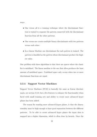
3.3.5 ψ -learning
ψ -learning is a variant of the SVM algorithm modied in order to generally
produce better results when faced with sparse non-linear separable training
sets [18]. The mathematical dierence lies within the cost function which,
17](https://image.slidesharecdn.com/sonaproject-111012233839-phpapp02/85/Sona-project-23-320.jpg)
![Figure 3.2: The ψ function used in the cost function, equation 3.10, for
ψ -learning training.
with quadratic programming as is the case with SVM [18].
19](https://image.slidesharecdn.com/sonaproject-111012233839-phpapp02/85/Sona-project-25-320.jpg)

![(a) Original (b) Scale = 15
(c) Scale = 30 (d) Scale = 45
Figure 4.2: Image at dierent scales.
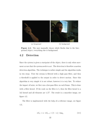
where ref n−1 is the previous reference image. The imgn is the current image
from the stream and α is a variable for tuning how fast the reference image
should adapt to changes. When subtracting the reference from the current
image, we will achive a value that describes the amount of change in color
at every pixel
diff n = imgn − ref n . (4.2)
A threshold is applied to the diff n image, reducing the noise, and at pixels
with valules = 0, some kind of motion is assumed, see gure 4.3. [1]
23](https://image.slidesharecdn.com/sonaproject-111012233839-phpapp02/85/Sona-project-29-320.jpg)
![(a) reference image, equation 4.1 (b) dierence image, equation 4.2
(c) motion detected
Figure 4.3: Results from the detection algorithm. Motion detected is
binary with ones where the dierence image has a value over a threshold
and zeros otherwise.
4.3 Recognition
To be able to track a specic object, motion detection is not sucient, since
the detection algorithm does not give any information regarding what is
moving. The Recognition block, see section 2.1, is responsible for recognizing
the object that is supposed to be tracked.
The recognition system in the present thesis is based on the system used
for video object segmentation in Liu et al [13]. The learning algorithm used
24](https://image.slidesharecdn.com/sonaproject-111012233839-phpapp02/85/Sona-project-30-320.jpg)
![B(−1,−1) B(−1,0) B(−1,1)
B(0,−1) B(0,0) B(0,1)
B(1,−1) B(1,0) B(1,1)
Figure 4.4: Neighbouring blocks of 9x9 pixels.
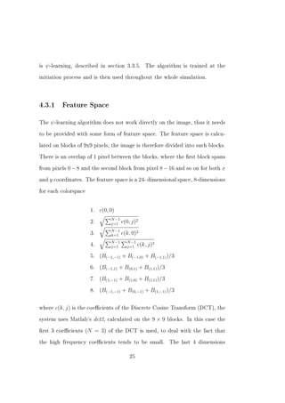
are the average color of the 9x9 neighboring blocks on each side, see gure
4.4. The combination of DCT and neighboring block color values gives good
classication of surface as well as grouping information which reduces the
impact of noise. [13]
4.3.2 Training
When the object is chosen as described in 4.1 the algorithm needs to be
trained by using the test data. The blocks that are not chosen is used as
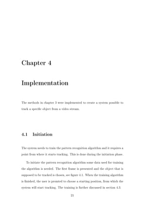
background, see gure 4.1. The training is done with Matlab's fminsearch.
fminsearch needs a start point in the feature space. This start point is
calculated using minimum squared error solution with the pseudoinverse
w = (AT A)−1 AT Y
where w is the weight vector, A is a matrix where each row represents a
training point and Y is a matrix containing rows with the corresponding
class for each training point.
26](https://image.slidesharecdn.com/sonaproject-111012233839-phpapp02/85/Sona-project-32-320.jpg)
![4.5 Prediction
A LMS-lter, see section 3.1.1, is used to predict the next point of interest,
which is used in the optimization of the system.
The LMS-lter is designed to be a one step ahead lter [10]. We want
to predict the next coordinate using previous observations. Two lters were
implemented, 1 for each coordinate:
N
x(n + 1) = θx (k)x(n − k)
k=0
N
y(n + 1) = θy (k)y(n − k).
k=0
During simulations the lter mostly kept the previous 6 (N = 6) coordinates
and µ was set around 10−8 .
4.6 Optimization
To make the system run faster, a number of constraints were added to the
system in order to reduce the work load.
The Detection described in section 4.2 is based on a lter which uses
earlier images. Therefore it is not suitable to reduce the work load only by
calculating parts of the image.
The task that generated the heaviest load on the computer was the con-
version from the pixel blocks to the feature space. In an study by Yi Liu
et al [13], which uses the same feature space, calculations of the DCT is the
major contributor for this load. Therefore two constraints needs to be ful-
28](https://image.slidesharecdn.com/sonaproject-111012233839-phpapp02/85/Sona-project-34-320.jpg)

![color space foreground error background error total error
RGB 0.76% 10.57% 8.84%
normalized RGB 1.82% 12.82% 11.26%
HSV 0.15% 10.57% 9.10%
TSL 5.77% 11.04% 10.30%
YCrCb 1.82% 13.52% 11.86%
NTSC 1.67% 7.17% 6.39%
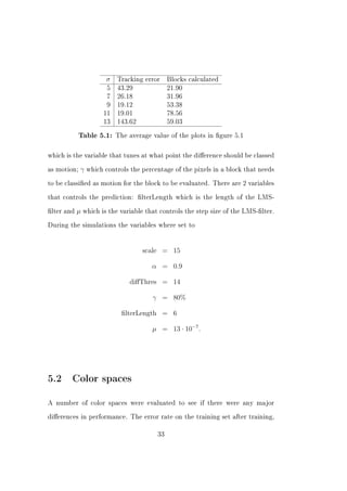
Table 5.2: Error rates of a number of colorspaces.
i.e. the amount of misclassications when trying to classify the training
set, is presented in table 5.2. The conversion from the RGB image was
done either with Matlab's built in functions, or as described in the study by
Sazonov [19]. The reason why the background has such high error rate is
that in the example in section 4.1, see gure 4.1, the face is not a part of
the object, but has similar features as the hand. The NTSC conversion, YIQ
color space is supplied by Matlab and were used most extensively during the
tests.
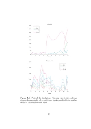
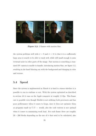
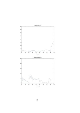
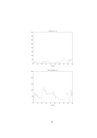
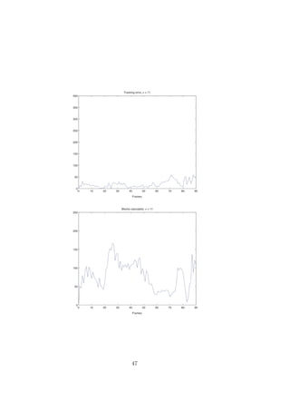
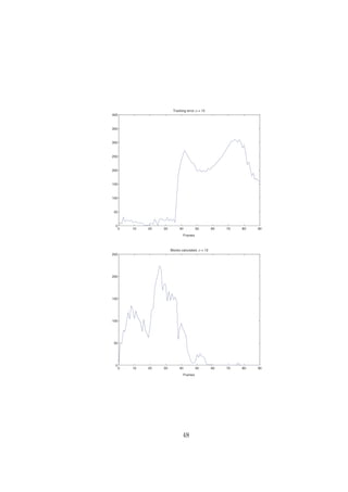
5.3 Tracking
During preferable conditions, such as sucient light and no or little distur-
bance in the background, the tracking worked well. The system still managed
when noise, such as back light and/or motion of other objects in the back-
ground was introduced. The lter allowed the system to work, even though
the tracking failed during small portions of time, but was able to snap on
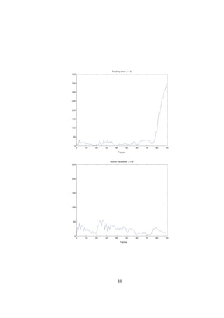
again after a few frames. Due to limitations in the system the tracking will
fail if a block is misclassied as the object, which only occurs if motion is
detected in the block. This occurs at frame 38 and σ = 13. The reason why
34](https://image.slidesharecdn.com/sonaproject-111012233839-phpapp02/85/Sona-project-40-320.jpg)

![Chapter 6
Discussion
The system works overall as expected. It outperforms advanced algorithms
in terms of lower computational power needed, and is more stable then the
fast ones. A drawback is that the system parameters were dependent on
the object and its surroundings. Much of the failure could probably be
compensated with more complex equipment. A more advanced camera could
be congured to use shorter shutter time, reducing the problem with tracking
failure during motion blur.
Problems due to limitations in the algorithms of the system is a more
complex problem. For example, when the tracker fails because of misclassi-
cation and motion, the problem will not be solved with better hardware.
Also if the object is big and has no texture so that it is registered as a at
surface, the motion algorithm will only detect motion on the contours, giving
a false representation of the object.
To improve the system, it might be possible to model the shape of the
object and feed that to an adaptive lter, such as the Kalman lter [10, 20].
37](https://image.slidesharecdn.com/sonaproject-111012233839-phpapp02/85/Sona-project-43-320.jpg)
![which describes how likely it is that X is set to x and Y is set to y (P (x, y)
and P (X = x, Y = y) is dierent notations for the same thing).
Conditional probability
PX|Y (x|y)
describes how likely it is that X is set to x given that Y is set to y (P (x|y) and
P (X = x|Y = y) is dierent notations for the same thing). The denition is
PX,Y (x, y)
PX|Y (x|y) = .
PY (y)
Bayes formula
If we have the knowledge of both PX (x) and PY |X (y|x), we can, from the
denition of conditional probability get
PX,Y (x, y) = PX|Y (x|y)PY (y)
= PY |X (y|x)PX (x),
which can be rewritten to
PX|Y (x|y)PY (y)
PY |X (y|x) = .
PX (x)
This is known as Bayes formula [2, 21].
40](https://image.slidesharecdn.com/sonaproject-111012233839-phpapp02/85/Sona-project-46-320.jpg)
![Expected value
The expected value is the mean value or function of the stochastic variable
or function
E[X] = mX
E[f (X)] = mf (X).
For a discrete stochastic variable the expected value is calculated
E[X] = xPX (x).
x∈X
Variance
The expected value gives the mean value of the stochastic variable or func-
tion. Variance gives the expected value of the squared distance between the
stochastic variable and mx
V ar[X] = σ 2 = E[(X − mx )2 ].
The variance can be expressed
V ar[X] = E[X 2 ] − (E[X])2
V ar[f (X)] = E[f 2 (X)] − (E[X])2 .
41](https://image.slidesharecdn.com/sonaproject-111012233839-phpapp02/85/Sona-project-47-320.jpg)
![Covariance
Covariance is dened as
rXY = V ar[XY ]
= E[(X − mX )(Y − mY )]
= (x − mX )(y − mY )PX,Y (x, y).
x∈X y∈Y
42](https://image.slidesharecdn.com/sonaproject-111012233839-phpapp02/85/Sona-project-48-320.jpg)

![Bibliography
[1] Rafael C. Gonzalez and Richard E. Woods, Digital Image Processing,
Prentice-Hall, Inc., second edition, 2001.
[2] Peter E. Hart Richard O. Duda and David G. Stork, Pattern Classi-
cation, Wiley Sons, Inc., second edition, 2001.
[3] Ville Kyrki and Danica Kragi¢, Tracking rigid objects using integration
of model-based and model-free cues, nyn, 2005.
[4] Nikolaos D. Doulamis, Anastasios D. Doulamis, and Klimis Ntalianis,
Adaptive classication-based articulation and tracking of video objects
employing neural network retraining, .
[5] Dorin Comaniciu, Visvanathan Ramesh, and Peter Meer, Kernel-based
object tracking, IEEE Trans. Pattern Anal. Mach. Intell., vol. 25, no.
5, pp. 564575, 2003.
[6] Aishy Amer, Voting-based simultaneous tracking of multiple video ob-
jects, 2003, vol. 5022, pp. 500511, SPIE.
[7] Danica Kragi¢, Visual Servoing for Manipulation: Robustness and In-
tegration Issues, Ph.D. thesis, Royal Institute of Technology, 2001.
49](https://image.slidesharecdn.com/sonaproject-111012233839-phpapp02/85/Sona-project-55-320.jpg)
![[8] A. Cavallaro, O. Steiger, and T. Ebrahimi, Tracking video objects in
cluttered background, IEEE Transactions on Circuits and Systems for
Video Technology, vol. 15, no. 4, pp. 575584, 2005.
[9] M. Gastaud, M. Barlaud, and G. Aubert, Tracking video objects using
active contours, in MOTION '02: Proceedings of the Workshop on
Motion and Video Computing, Washington, DC, USA, 2002, p. 90, IEEE
Computer Society.
[10] Håkan Hjalmarsson and Bjorn Ottersten, Lecture notes in adaptive
signal processing, Tech. Rep., Signal, Sensors and System, Stockholm,
Sweden, 2002.
[11] Benny Rousso Michal Irani and Shmuel Peleg, Computing occluding
and transparent motions, Tech. Rep., Institute of Computer Science,
Jerusalem, Israel, 1994.
[12] Christopher J. C. Burges, A tutorial on support vector machines for
pattern recognition, Data Mining and Knowledge Discovery, vol. 2, no.
2, pp. 121167, 1998.
[13] Yi Liu and Yuan F. Zheng, Video object segmentation and tracking
using ψ -learning, IEEE Transactions on Circuits and System for Video
Technology, 2005.
[14] Constantine Kotropoulos Anastasios Tefas and Ioannis Pitas, Using
support vector machines to enhance the performance of elastic graph
matching for frontal face authentication, IEEE Trans on Pattern Anal.
Mach. Intell., 2001.
50](https://image.slidesharecdn.com/sonaproject-111012233839-phpapp02/85/Sona-project-56-320.jpg)
![[15] Daniel J. Sebald and James A. Bucklew, Support vector machine tech-
niques for nonlinear equalization, IEEE Transactions on Signal Pro-
cessing, 2000.
[16] Robert Freund Edgar Osuna and Federico Girosi, Training support
vector machines: an application to face detection, IEEE, Computer
Vision and Pattern Recognition, 1997.
[17] Massimiliano Pontil and Alessandro Verri, Support vector machines
for 3d object recognition, IEEE Transactions on Pattern Anal. Mach.
Intell., 1998.
[18] Xuegong Zhang Xiaotong Shen, George C. Tseng and Wing Hung Wong,
On ψ -learning, Journal of the American Statistical Association, 2003.
[19] Vassili Sazonov Vladimir Vezhnevets and Alla Andreeva, A survey on
pixel-based skin color detection techniques, Tech. Rep., Graphics and
Media Laboratory, Faculty of Computational Mathematics and Cyber-
netics, Moscow, Russia, 2003.
[20] Monson H. Hayes, Statistical Digital Signal Processing and Modeling,
Wiley Sons, Inc., rst edition, 1996.
[21] Arne Leijon, Pattern recognition, Tech. Rep., Signal, Sensors and
System, Stockholm, Sweden, 2005.
51](https://image.slidesharecdn.com/sonaproject-111012233839-phpapp02/85/Sona-project-57-320.jpg)

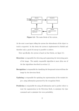
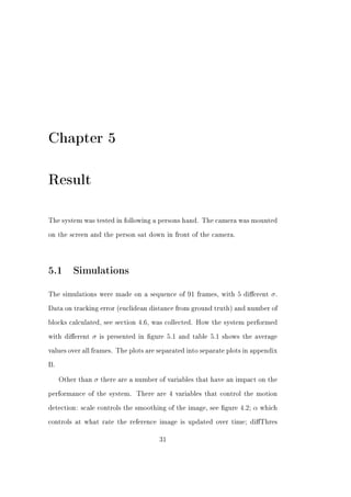
This document summarizes a master's thesis project that aimed to implement an object tracking system in Matlab using a single webcam. The system uses both fast and advanced algorithms to achieve better accuracy and speed than either approach alone. It tracks a person's hand placed in front of the webcam mounted on a computer screen. While not real-time, it serves as an initial step towards a real-time capable system. The thesis discusses background on object tracking approaches, related work, the specific problem and hardware, methods used including adaptive filtering, motion detection and pattern recognition, implementation details, results of simulations and tracking tests, and ideas for future work.


![wronski_ugthesis[1]](https://cdn.slidesharecdn.com/ss_thumbnails/95db93fc-5f15-4802-985f-832034d277d7-150202014804-conversion-gate02-thumbnail.jpg?width=640&height=640&fit=bounds)