Lyapunov stability analysis in analog and digital control system.

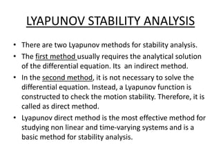
1. LYAPUNOV STABILITY ANALYSIS
• There are two Lyapunov methods for stability analysis.
• The first method usually requires the analytical solution
of the differential equation. Its an indirect method.
• In the second method, it is not necessary to solve the
differential equation. Instead, a Lyapunov function is
constructed to check the motion stability. Therefore, it is
called as direct method.
• Lyapunov direct method is the most effective method for
studying non linear and time-varying systems and is a
basic method for stability analysis.

2. SECOND METHOD OF LYAPUNOV
STABILITY
• The second method is based on a the fact that
if the system has an asymptotically stable
equilibrium state, then the stored energy of
the system displaced within a domain of
attraction decays with increasing time until it
finally assumes its minimum value at the
equilibrium state.

3. LYAPUNOV STABILITY ANALYSIS
• Lyapunov stability is used to described the stability of a
dynamic system.
• Lyapunov stability for linear time invariant system,
X˙=Ax
is Lyapunov stable if no eigenvalues of a are in the right
half of the complex plane.
• Lyapunov introduced the lyapunov function,
• But before discussing the lyapunov function, it is
necessary to define the definiteness of scalar function.

4. DEFINITENESS OF SCALAR FUNCTION
• Positive definite of function-
V(x1,x2,x3…xn) >0
for any non zero value of x1,x2,x3…xn
• Negative definite of function-
V( x1,x2,x3,…xn) <0
For any non zero value of x1,x2,x3…xn
• Positive semi definite of function-
V(x1,x2,x3…xn) ≥0
For any non zero value of x1,x2,x3,…xn
• Negative semi definite of function-
V(x1,x2,x3,…xn)≤0
For any non zero value of x1,x2,x3,…xn

5. Stability in the sense of Lyapunov
• An equilibrium state xe of an autonomous
system is stable in the sense of Lyapunov, if
corresponding to each S(ε), there is an S(δ)
such that trajectories starting in S(δ) do not
leave S(ε) as time increases indefinitely.

6. Asymptotic stability
• An equilibrium state xe of the system is said to
be asymptotically stable in the sense of
Lyapunov if every solution starting within S(δ)
converges, without leaving S(ε), to xe as time
increases indefinitely.

7. Instability
• An equilibrium state xe is said to be unstable if
for some real number ε>0 and any real
number δ>0, no matter how small, there is
always a state x0 in S(δ) such that the
trajectory starting at this state leaves S(ε).

8. Stability of continuous-time linear
system
Consider a linear system described by the state equation-
x˙=Ax
Where A is n×n real constant matrix.
The linear system is asymptotically stable at the origin if,
for any given symmetric positive definite matrix Q,
there exists a symmetric positive definite matrix P, that
satisfies the matrix equation-
A’P+PA = -Q
We may choose Q=I, the identity matrix.

9. Example-
Let us determine the stability of the system described
by the following equation
x˙ = Ax
With
Solution-
Equation for P-
A’P + PA = -I

10. After solving, we get the equations-
And solving for P
We obtain
By using Sylvester’s test, we find that P is positive
definite.
P1= (23/60)>0 and P2= (17/300)>0
Therefore, the system is consider as asymptotically
stable at origin.

11. Stability of discrete-time linear system
Consider a linear system described by the state
equation-
x(k+1) = Fx(k)
Where F is n×n real constant matrix.
The linear system is asymptotically stable at the
origin if, for any given symmetric positive definite
matrix Q, there exists a symmetric positive
definite matrix P, that satisfies the matrix
equation-
F’PF – P = -Q
Here also we may choose Q=I, the identity matrix.

12. Example
Let us determine the stability of the system described
by the following equation-
x(k+1) = Fx(k)
With
Solution-
Solving the equation for P-
F’PF – P = -I

13. After solving we get the equations-
Solving for P
By using Sylvester’s test, we find that P is negative
definite.
P1= (-43/60)<0
P2= (-1/49)<0
Therefore, the system is unstable.