The document discusses three increasingly sophisticated Monte Carlo algorithms - Variational Monte Carlo (VMC), Diffusion Monte Carlo (DMC), and Diffusion Monte Carlo with Importance Sampling (DMC-IS) - for studying quantum systems computationally. It applies these algorithms to the harmonic oscillator as a test case. VMC converges to the correct energy when using the exact wavefunction. DMC shows large fluctuations in results. DMC-IS gives stable results, correctly obtaining the exact energy when using the exact wavefunction as the trial function, and a close approximation when using a similar but slightly incorrect trial function.

1. Application of Monte Carlo Methods to Study Quantum Systems
Jacob Deal
Many body systems are typically impractical for analytical study, meriting computational tech-
niques. Development and implementation of accurate efficient algorithms are critical as systems
become increasingly larger and complex. Monte Carlo methods are one such family of algorithms
that have been shown to be both efficient and accurate when applied to the systems. Three increasingly
sophisticated Monte Carlo algorithms will be discussed in detail, and applied to study the perturbed
and unperturbed Harmonic Oscillators. Comparison of the results between and within the differ-
ent algorithms will be done to further verify efficiency and accuracy. Finally the next steps in 3D
implementation for multi-particle systems will be discussed.
CONTENTS
I. Introduction 1
II. Methods 2
A. Metropolis Algorithm 2
B. Variational Monte Carlo 2
C. Diffusion Monte Carlo 3
D. Diffusion Monte Carlo with Importance
Sampling 4
III. Results 5
A. Study of the Harmonic Oscillator 5
B. Study of a Perturbed Harmonic
Oscillator 6
IV. Discussion 6
References 7
Apendix: Code 7
A. ISDMC.m 7
B. DiffusionMonteCarlo.m 11
I. INTRODUCTION
Study of many body systems is essential to mod-
ern chemistry and solid state physics. To analyti-
cally calculate the wavefunctions and relevant quan-
tities from a quantum mechanical foundation is at
the very least nontrivial, and often impossible. Com-
putational methods have become a major tool to
complement experimental methods, as numerical al-
gorithms are more manageable than attempting the
analytic approach. Even so, as more particles are in-
volved in calculations and higher resolutions and ac-
curacies are desired the computational difficulty and
resource requirements increase rapidly. Develop-
ment of more efficient and sophisticated algorithms
that can better handle these systems is a key com-
ponent to solving these computational issues, since
software is more malleable than hardware. One fam-
ily of such methods is known as Monte Carlo simula-
tions, which use randomized sampling of the desired
configuration space to simulate systems. To build a
more sophisticated Monte Carlo Algorithm that can
handle complex quantum mechanical systems starts
simply. Usage of a Diffusion Monte Carlo algorithm
that implements Importance Sampling has been pro-
posed for modeling solids and other many-body sys-
tems. Working on a foundation of a basic Metropo-
lis Algorithm for sampling a quantum system, three
increasingly sophisticated Monte Carlo Algorithms
have been developed to study solids [1].
In order of sophistication these algorithms are
the Variational, Diffusion, and Diffusion with Impor-
tance Sampling algorithms. The Variational method
is essentially the bare bones Metropolis Algorithm
implemented for a quantum system, but has the key
feature of utilizing a trial wavefunction ψT that is
used as an estimate for sampling the configuration
space. The Diffusion method differs in that it de-
stroys Metropolis walkers in regions of large poten-
tial and proliferates walkers in regions of low poten-
tial. This biasing makes it very efficient in sampling
a configuration space without using a trial wavefunc-
tion as in the Variational method. The most sophis-
ticated of the three methods acts to combine them,
and yet adds another feature: Importance Sampling.
The algorithm looks at the gradient of ψT to not
only bias walkers to regions of low potential, but to
regions of large ψT as well. Further, the method
implements a nodal surface feature that prevents
walkers from crossing into regions where ψT changes
sign and further increasing the efficiency of the al-
gorithm. Applying these algorithms to unperturbed
and perturbed Harmonic Oscillators, their features
and behavior will be studied and compared.

2. FIG. 1. A flow diagram depicting how a simple Metropo-
lis Algorithm operates.
II. METHODS
A. Metropolis Algorithm
The Metropolis Algorithm is the backbone
of both Variational and Diffusion based Quantum
Monte Carlo methods. The algorithm itself is simple
and depicted in Figure 1. A walker or set of walkers
are initiated with position R according to some ini-
tial distribution. Each walker is then stepped to a
new position R by randomly sampling a given prob-
ability distribution T, and the set of new positions
are labeled as ”trial” positions. A probability that
the walker proceeds from R to R is then calculated
for the walker given by
A(R ← R) = Min 1,
T(R ← R )D(R )
T(R ← R)D(R)
(1)
where D is defined as an importance function that
determines the relative ”strength” of a given position
[1].
FIG. 2. A flow diagram for the VMC Algorithm, apply-
ing the Metropolis Algorithm with a measurement step
at the end.
B. Variational Monte Carlo
T he Variational Monte Carlo Method (VMC)
is essentially the basic Metropolis Algorithm, but
with specific function D and T and a measurement
step. A flow diagram of the simple VMC algorithm
is found in Figure 2.
For quantum systems that obey the Schrdinger
Wave Equation ˆHΨ = EΨ and are well defined, the
probability density function T in the Metropolis Al-
gorithm becomes a Gaussian centered over zero. A
trial wave function ψT (R) is used to approximate Ψ
for energy and probability calculations. The func-
tion D is defined by
D(R) =
|ψT (R)|2
|ψT (R)|2dR
(2)
which is naturally the probability density of ψT eval-
uated at the point R. In order to calculate energies,
the local energy EL is used to calculate average en-
ergy Ev for a given set of positions {R}. The equa-
2

3. tions for these are given by
EL(R) =
ˆHψT (R)
ψT (R)
(3)
Ev ≈
1
M
M
m=1
EL(Rm) (4)
With these specific functions, the probability factor
A in Eq. 1 utilizes Gaussian functions as T and the
particle density function D to accept or reject steps.
The function T is also used to step the walkers in a
random direction. Choice of the standard deviation
in T is decided by tuning it until the acceptance ratio
is approximately .5.
Exact details on the derivation of these equa-
tions can be found in [1]. After a given number of
time steps the distribution of {R} will equilibrate,
although this can take a long time depending on
the quality of ψT , the initial distribution of walkers,
and the complexity of the potential V in the Hamil-
tonian. Once the value of Ev has become stable
over a desired number of time steps, the algorithm
is terminated. Typically, VMC will give a some-
what accurate estimate of the ground state energy
and functional form; although the efficiency is very
small compared to more sophisticated methods and
is heavily dependent upon the accuracy of ψt and a
number of other factors.
C. Diffusion Monte Carlo
The Diffusion Monte Carlo algorithm again ex-
pands upon the Metropolis Algorithm but has a key
difference. Instead of the probability factor A be-
ing used to calculate whether a trial step will be
accepted, a weighting factor P is used. Further, a
birth/death algorithm is introduced. A flow diagram
of a simple DMC algorithm is shown in Figure 3.
The weighting factor P is given by
P = e−dt(V (R)+V (R )−2ET )/2
(5)
where dt is the time step size and ET is defined as the
trial energy. The algorithm starts just as VMC did,
but now the factor P is calculated for each walker.
Then, a birth/death algorithm is used to either de-
stroy or create walkers by utilizing P. The number
of new walkers proceeding at the new position R is
given by
Mnew = floor[P + η] (6)
where η is random number uniformly distributed on
[0, 1]. When the potential V is large, the factor P
FIG. 3. A flow diagram for a DMC algorithm using
a birth/death algorithm. In regions of large potential
V , the weighting ratio P approaches 0 and vice versa.
This means that walkers die in regions of large V and
proliferate in regions of small V .
will be relatively small. Similarly, when V is small,
the factor P will be large. This means that in re-
gions of high V walkers are more likely to be killed
off, while in regions of low V walkers are likely to
proliferate. Thus, diffusion of the walkers is biased
towards regions of lower V and will converge to the
steady state relatively quickly.
One side effect of the birth/death algorithm is
the potential for uncontrolled population growth or
death. In order to maintain a relatively stable pop-
ulation about some mean value, the trial energy ET
is adjusted at each time step to counteract the pop-
ulation change. A simple method for doing this is
to take the ratio of current number of walkers m to
3

4. the desired average population size Mavg and use it
in
ET ← ET − C ln( m
Mavg
) (7)
The parameter C sets how quickly the population
responds to changes in ET , and should be tuned such
that the population returns to the average every 10
to 50 steps [1].
While this algorithm is efficient compared to
VMC, it does have its draw backs. First, the trial en-
ergy as an estimate will vary quite a bit over time,
even averaging over time. Second, the population
can become unstable even with the method proposed
above over a long enough period of time. It does,
however, produce a ground state energy that is more
accurate than with VMC, and the functional form is
more accurate and stable as well.
D. Diffusion Monte Carlo with Importance
Sampling
DMC with Importance Sampling essentially
combines all of the previous techniques discussed,
with two new additions. The concept of nodal sur-
faces, and Importance Sampling is introduced are in-
corporated to further increase efficiency. The nodal
surface of a given walker space {R} is simply put
the regions where the wave function changes sign.
Since the wavefunction changes sign at the nodes,
the walkers are not permitted to cross the bound-
ary and can be rejected to prevent walker exchange
between nodal regions and treat the regions inde-
pendently of each other. Importance sampling uti-
lizes the trial wavefunction ψT to act as a sort of
estimate of the ground state for a given potential
in order to bias the walkers to regions of large |ψ2
T |.
This compounds the biasing used in normal DMC by
looking at how the potential and trial wavefunction
behave together in order to bias more efficiently. A
flow diagram of the algorithm is given in Figure 4.
In order to bias the walkers to regions of large ψT ,
ψT is used to determine a drift velocity that is in-
corporated at multiple steps. This drift velocity is
calculated via
vd =
ψT (R)
ψT (R)
(8)
The Probability factor as defined in the Metropo-
lis Algorithm Eq. 1 is used, but a new function is
used instead of the Gaussian that utilizes vd. This
FIG. 4. A flow diagram of the DMC algorithm incorpo-
rating an initial VMC relaxation phase and Importance
Sampling.
function is labeled as Gd and is given by
Gd(R ← R , dt)
= (2πdt)−3N/2
exp −
[R − R − dtvd(R )]2
2dt
(9)
Defining a probability of acceptance factor paccept
paccept(R ← R )
= Min 1,
Gd(R ← R, dt)ψT (R)2
Gd(R ← R , dt)ψT (R)2
]
(10)
Up to this point the algorithm first calculates the
drift velocities of walkers finds the trial positions via
R = R + χ + dtvd(R ) (11)
where χ is a number randomly sampled from a Gaus-
sian centered on zero with σ =
√
dt. Next, the
walker is checked against the trial wavefunction ψT
to see if it crossed a nodal boundary and rejects the
step if it has. The probability factor for each of these
trial steps is calculated via Eq. 10 and steps are re-
jected according to Metropolis rejection/accepting.
The remainder of the Importance Sampling al-
gorithm is identical to DMC, only with a small
change in the weighting factor used in Birth/Death.
The new weighting factor is labeled Gb and is given
4

5. by
Gb(R ← R , dt)
= exp − dt
EL(R) + EL(R ) − 2ET
2
(12)
Note that this weighting factor is identical to the
DMC version in Eq. 5, except V has been replaced
with the local energy EL. This has the benefit of
smoothing out many of the fluctuations in the pop-
ulation and as an end result creates a more stable
energy. The walkers are birthed and killed as they
were before, only with this new weighting function
that incorporates both V and ψT . The population
is also adjusted in the same manner as before by
adjusting ET [1].
The algorithm can be made more efficient by
starting with a distribution of walkers that closely
approximates the ground state and choosing an en-
ergy ET that is approximately close to the ground
state. This is done by relaxing the distribution us-
ing a VMC method for a set amount of time before
feeding the resulting walker distribution and energy
to the Importance Sampling Algorithm. The system
is then allowed to come to equilibrium and stopped
when the uncertainties in the energy Ev are at the
desirable size.
III. RESULTS
A. Study of the Harmonic Oscillator
In order to understand the operational parameters
of the previously described algorithms, the harmonic
oscillator was used as a study case. This system was
chosen because it well understood, contains a simple
potential V = .5x2
, and has a simple ground state in
the form of a Gaussian with σ =
√
2. The amplitude
of the wavefunction itself does not matter here due to
the linear nature of the Schrdinger Wave Equation
causing a linear scaling factor, meaning that nor-
malization can be performed after the fact without
needing to do so during calculations. The results of
the Variational Monte Carlo Algorithm are depicted
in Figure 5, where the trial wavefunction used is the
exact ground state. This serves as a test of how well
the algorithm behaves with the exact ground state
as ψT . Note that the ground state energy immedi-
ately converges to the exact value of Eexact = .5.
The functional form is also approximately correct,
although it is slightly off.
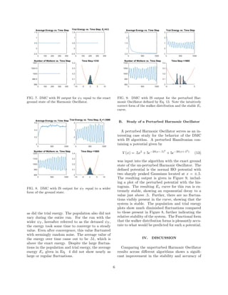
FIG. 5. Program output of the VMC algorithm applied
to the Harmonic Oscillator using the exact ground state
as a trial wavefunction.
FIG. 6. DMC output for the Harmonic Oscillator. Note
the large fluctuations in the population, ET , and Eavg.
Running the Harmonic Oscillator through the
DMC algorithm resulted in the output given by Fig-
ure 6. The output of the DMC algorithm shows large
fluctuations in both ET and Eavg, despite the very
nice and stable distribution of walkers. Even at large
time steps for which the average is over a long time,
fluctuations are large enough to be undesirable.
In order to study how DMC with Importance
Sampling handles the Harmonic Oscillator, two dif-
ferent trial wavefunctions were used. Both were
Gaussians centered on zero, but the differed in the
standard deviations. One was σ =
√
2 correspond-
ing to the exact ground state, and the other was
σ = 2
√
2 corresponding to something wider than the
exact ground state. The resulting program outputs
are displayed in Figures 7 and 8. Comparing the
results with the slightly different ψT ’s shows an in-
teresting feature of the algorithm. The exact ground
state run immediately sat at the exact energy of .5,
5

6. FIG. 7. DMC with IS output for ψT equal to the exact
ground state of the Harmonic Oscillator.
FIG. 8. DMC with IS output for ψT equal to a wider
form of the ground state.
as did the trial energy. The population also did not
vary during the entire run. For the run with the
wider ψT , hereafter referred to as the detuned ψT ,
the energy took some time to converge to a steady
value. Even after convergence, this value fluctuated
with seemingly random noise. The average value of
the energy over time came out to be .51, which is
above the exact energy. Despite the large fluctua-
tions in the population and trial energy, the average
energy Ev given in Eq. 4 did not show nearly as
large or regular fluctuations.
FIG. 9. DMC with IS output for the perturbed Har-
monic Oscillator defined by Eq. 13. Note the intuitively
correct form of the walker distribution and the stable Ev
curve.
B. Study of a Perturbed Harmonic Oscillator
A perturbed Harmonic Oscillator serves as an in-
teresting case study for the behavior of the DMC
with IS algorithm. A perturbed Hamiltonian con-
taining a potential given by
V (x) = .5x2
+ 5e−20(x−.5)2
+ 5e−20(x+.52
)
(13)
was input into the algorithm with the exact ground
state of the un-perturbed Harmonic Oscillator. The
defined potential is the normal HO potential with
two sharply peaked Gaussians located at x = ±.5.
The resulting output is given in Figure 9, includ-
ing a plot of the perturbed potential with the his-
togram. The resulting Ev curve for this run is ex-
tremely stable, showing an exponential decay to a
value just above .5. Further, there are no fluctua-
tions visibly present in the curve, showing that the
system is stable. The population and trial energy
plots show much diminished fluctuations compared
to those present in Figure 8, further indicating the
relative stability of the system. The Functional form
that the walker distribution forms is pleasantly accu-
rate to what would be predicted for such a potential.
IV. DISCUSSION
Comparing the unperturbed Harmonic Oscillator
results across different algorithms shows a signifi-
cant improvement in the stability and accuracy of
6

7. the resulting values of Ev and walker distributions.
Even for the ”detuned” ψT used in the DMC with
IS run, the fluctuations are much improved and the
energy value much more acceptable than the normal
DMC result. These results also agree with the Vari-
ational Principle, as none of the final energies pro-
duced were below the exact ground state energy .5.
The result of the perturbed Harmonic Oscillator was
very surprising in its stability and final energy value
at just above .5. The perturbed result also agrees
with the variational principle, as the perturbed po-
tential would be expected to be at the very least .5
and probably only slightly above that. Further, the
functional forms for all of the DMC with IS results
were visually accurate and stable.
The next step in studying these algorithms and
applying them is to extend the coded algorithms
to 3D. This should not present to daunting of a
task, as the algorithms don’t include much inter-
play across dimensions. After 3D has been achieved,
Application to a nontrivial system would be per-
formed. Such a system would be the H−
ion, which
would also require extension to a two particle sys-
tem. While the modification of the algorithms is
not too difficult, the implementation would prove to
be more difficult as care must be taken to insure
the proper referencing and indexing of arrays is per-
formed. Based on the Harmonic Oscillator studies
performed here, the resulting outputs are expected
to be fairly accurate and reflective of the true re-
sult given that ψT is chosen appropriately. Further
study into what merits a ”good” ψT is warranted for
this reason so that the resulting wavefunction isn’t
overly detuned.
[1] W.M.C Foulkes, L. Mitas, R. J. Needs, and G. Ra-
jagopal, 2001, Quantum Monte Carlo simulations of
solids, Rev. Mod. Phys. 73, 33.
APENDIX: CODE
A. ISDMC.m
close all
clear
clc
%%%%%%%%%%%%%%%%%%%%% General Parameter Definitions %%%%%%%%%%%%%%%%%%%%%%%
N=1000; % Number of Walkers (Initial)
b=[1,sqrt(2.0)]; % Trial Wave Function parameters
h=1; % Planck’s Constant
mass=1; % mass
D=(h^2)/(2*mass); % Diffusion Constant / Hamiltonian term
dt=.01; % Time Step
%%%%%%%%%%%%%%%%%%%%%% General Function Definitions%%%%%%%%%%%%%%%%%%%%%%%%
% Function Definitions for V and PsiT
V=@(r) .5.*r.^2 + 5.*exp(-20.*(r-.5).^2)+5.*exp(-20.*(r+.5).^2);
psiT=@(r,b) b(1).*exp(-(r./b(2)).^2);
% Defintion of the Hamiltonian %
% Use the commands syms r; psiT(r)=[insert function]; diff(psiT,r,2)
% before running and manually enter for speed reasons. Otherwise, it does
% it every iteration. A ’.’ must also be inserted before every ’^’, ’*’ and
% ’/’ to allow for array usage.
D2psiT=@(r,b)((4.*r.^2.)./b(2)^4 - (2./b(2)^2)).*psiT(r,b);
HpsiT=@(r,b)(-D.*D2psiT(r,b))+V(r).*psiT(r,b);
7

8. % The local energy function
El=@(r,b) HpsiT(r,b)./psiT(r,b);
%%%%%%%%%%%%%%%%% VMC Algorithm for variation of PsiT%%%%%%%%%%%%%%%%%%%%%%
% VMC Parameters
Tv=50; % Recording time for VMC
muv=0; % mu for Metropolis in VMC
sigmav=1.45; % sigma for Metoropolis in VMC
% Function definitions for VMC
P=@(r,rvec,b) (psiT(r,b).^2)./sum((psiT(rvec,b)).^2);
A=@(r,rp,rvec,b) min(1,(normpdf(rp-r)./normpdf(r-rp)).*(P(rp,rvec,b)./P(r,rvec,b)));
% Walker Array Initialization
x=linspace(-5,5,N);
pos=ceil(psiT(x,b).^2);
r=zeros(sum(pos),2);
for i=1:N
r(sum(pos(1:i))-pos(i)+1:sum(pos(1:i)),:)=x(i);
end
N1=length(r);
% r=zeros(N,2);
% r(:,1)=normrnd(muv,sigmav,[N,1]);
% VMC Array Initialization
Ev=zeros(Tv,1);
Ev(1)=mean(El(r(:,1),b));
Ev(2)=Ev(1);
% The main loop for VMC.
for t=3:Tv
% Metropolis Walk update
rt=r(:,1)+normrnd(muv,sigmav,[N,1]);
% Acceptance algorithm
for n=1:N
if rand()<A(r(n,1),rt(n),r(:,1),b)
r(n,2)=rt(n);
else
r(n,2)=r(n,1);
end
end
r(:,1)=r(:,2);
Ev(t)=mean(El(r(:,1),b));
% Plotting for VMC
hold on
figure(1)
clf
subplot(2,1,1)
plot(Ev(1:t))
8

9. title([’E_v=’ num2str(Ev(t))]);
subplot(2,1,2)
title([’Time Step =’ num2str(t)])
histogram(r(:,1),’Normalization’,’probability’)
drawnow
end
%%%%%%%%%%%%%%%%%% Importance Sampling DMC Algorithm %%%%%%%%%%%%%%%%%%%%%%
% DMC Parameters
Mavg=1000; % Desired average number of walkers
T=1000; % Maximum run time
C=1; % Population control constant
sig=sqrt(2*D*dt); % Std. Dev. for Metropolis
Et=mean(Ev); % Assign Et based on VMC result
% DMC Function Definitions
Gd=@(r,rp,N,vdp) (((2*pi*dt).^(-3*N/2))).*exp(-((r-rp-dt.*vdp).^2)./(2*dt));
Gb=@(r,rp,Et,b) exp(-dt.*(El(r,b)+El(rp,b)-2*Et)./2);
Av=@(r,rp,N,b,vd,vdp) min(1,(Gd(r,rp,N,vd)./Gd(rp,r,N,vdp)).*((psiT(r,b).^2)./(psiT(rp,b).^2)));
% As with the VMC, determine vd=(1/psiT)*del(psiT)
vd=@(r,b) (-(2.*r)./b(2)^2);
% DMC Array Initialization
NumWalks=zeros(T,1);
NumWalks(1)=length(r(:,1));
E=zeros(T,1);
E(1)=Et;
Eavg=zeros(T,1);
Eavg(1)=mean(El(r(:,1),b));
vds=vd(r(:,1),b);
vdsp=vds;
% Main Loop
for t=2:T
% Update the new number of walkers
N=length(r(:,1));
% Calculate drift velocity
vds=vd(r(:,1),b);
% Metropolis walk
r(:,2)=r(:,1)+normrnd(0,sig,[N,1])+dt.*vds;
% Calculate new drift velocity
vdsp=vd(r(:,2),b);
% Check Nodal Crossing
for n=1:N
if psiT(r(n,1),b)*psiT(r(n,2),b)<0
r(n,2)=r(n,1);
else
9

10. if rand()<Av(r(n,1),r(n,2),N,b,vdsp(n),vds(n))
r(n,2)=r(n,1);
end
end
end
% Calculate the Birth/Death weighting factor and number of new walkers
Pv=Gb(r(:,1),r(:,2),Et,b);
M=floor(Pv+rand(N,1));
rt=r;
% Populate rt with the number of copies as updated by M
n=1;
while n<N
if M(n)==0
rt(n,:)=[];
M(n)=[];
n=n-1;
N=N-1;
end
n=n+1;
end
r=rt;
m=sum(M);
rt=zeros(m,2);
for n=1:N
rt(sum(M(1:n))-M(n)+1:sum(M(1:n)),:)=repmat(r(n,:),M(n),1);
end
% Assign rt to r and adjust Et to control population
r=[rt(:,2),rt(:,2)];
Et=Et-C*log(m/Mavg);
% Measurement
E(t)=Et;
Eavg(t)=mean(El(r(:,1),b));
NumWalks(t)=N;
% Plotting for VMC
if rem(t,1)==0
figure(2)
clf
hold on
subplot(2,2,1)
plot(Eavg(1:t))
title(’Average Energy vs. Time Step’)
subplot(2,2,2)
plot(E(1:t))
title(’Trial Energy vs. Time Step’)
subplot(2,2,3)
plot(NumWalks(1:t))
title(’Number of Walkers vs. Time Step’)
hold off
subplot(2,2,4)
10

11. hold on
title([’Time Step =’ num2str(t)])
histogram(r(:,1),30,’Normalization’,’probability’);
plot(x,(.25e-1)*V(x))
%plot(x,(.15).*psiT(x,b).^2)
xlim([-5,5])
hold off
drawnow
end
end
B. DiffusionMonteCarlo.m
close all
clear
clc
N=2.5e3;
Mavg=2.5e3;
T=10000;
C=10;
h=1;
mass=1;
D=(h^2)/(2*mass);
dt=.01;
sig=sqrt(2*D*dt);
Et=.5;
U=@(x) .5.*x.^2;
init=@(x) 2.*x./x;
x=linspace(-10,10,N);
pos=ceil(init(x));
r=zeros(sum(pos),2);
for i=1:N
r(sum(pos(1:i))-pos(i)+1:sum(pos(1:i)),1)=x(i);
end
% x=linspace(-10,10,N);
% r=zeros(N,2);
% r(:,1)=normrnd(0,3,[N,1]);
E=zeros(T,1);
E(1)=Et;
Eavg=zeros(T,1);
Eavg(1)=Et;
NumWalks=zeros(T,1);
NumWalks(1)=length(r(:,1));
for t=2:T
N=length(r(:,1));
11

12. r(:,2)=r(:,1)+normrnd(0,sig,[N,1]);
P=exp(-dt.*(U(r(:,2))+U(r(:,1))-2*Et)./2);
M=floor(P+rand(N,1));
rt=r;
n=1;
while n<N
if M(n)==0
rt(n,:)=[];
M(n)=[];
n=n-1;
N=N-1;
end
n=n+1;
end
r=rt;
m=sum(M);
rt=zeros(m,2);
for n=1:N
rt(sum(M(1:n))-M(n)+1:sum(M(1:n)),:)=repmat(r(n,:),M(n),1);
end
r=[rt(:,2),rt(:,2)];
if rem(t,1)==0 && t>101
hold on
clf
figure(1)
subplot(2,2,1)
plot(Eavg(t-101:t-1))
title(’Value of E_{avg} vs. Time Step’)
legend(num2str(mean(Eavg(t-101:t-1))))
subplot(2,2,2)
plot(E(t-101:t-1))
title(’Value of E_t vs. Time Step’)
subplot(2,2,3)
plot(NumWalks(t-101:t-1))
title(’Number of Walkers vs. Time Step’)
subplot(2,2,4)
hold off
hold on
title([’Time=’ num2str(t-1)])
histogram(r(:,1),40,’Normalization’,’probability’);
plot(x,(1e-2)*U(x))
xlim([-10,10])
hold off
drawnow
end
Et=Et-C*log(m/Mavg);
E(t)=Et;
Eavg(t)=mean(E(1:t));
NumWalks(t)=N;
end
12