Download to read offline
![Course “Fundamentals of Structural Dynamics”
An-Najah National University
April 19 - April 23, 2013
Lecturer: Dr. Alessandro Dazio, UME School
A. Dazio, April 19, 2013 Page 1/2
Fundamentals of Structural Dynamics
1 Course description
Aim of the course is that students develop a “feeling for dynamic problems” and acquire the theoretical
background and the tools to understand and to solve important problems relevant to the linear and, in
part, to the nonlinear dynamic behaviour of structures, especially under seismic excitation.
The course will start with the analysis of single-degree-of-freedom (SDoF) systems by discussing: (i)
Modelling, (ii) equations of motion, (iii) free vibrations with and without damping, (iv) harmonic, pe-
riodic and short excitations, (v) Fourier series, (vi) impacts, (vii) linear and nonlinear time history anal-
ysis, and (viii) elastic and inelastic response spectra.
Afterwards, multi-degree-of-freedom (MDoF) systems will be considered and the following topics will
be discussed: (i) Equation of motion, (ii) free vibrations, (iii) modal analysis, (iv) damping, (v) Rayleigh’s
quotient, and (vi) seismic behaviour through response spectrum method and time history analysis.
To supplement the suggested reading, handouts with class notes and calculation spreadsheets with se-
lected analysis cases to self-training purposes will be distributed.
Lecturer: Dr. Alessandro Dazio, UME School
2 Suggested reading
[Cho11] Chopra A., “Dynamics of Structures”, Prentice Hall, Fourth Edition, 2011.
[CP03] Clough R., Penzien J., “Dynamics of Structures”, Second Edition (revised), Computer and
Structures Inc., 2003.
[Hum12] Humar J.L., “Dynamics of Structures”. Third Edition. CRC Press, 2012.
3 Software
In the framework of the course the following software will be used by the lecturer to solve selected ex-
amples:
[Map10] Maplesoft: “Maple 14”. User Manual. 2010
[Mic07] Microsoft: “Excel 2007”. User Manual. 2007
[VN12] Visual Numerics: “PV Wave”. User Manual. 2012
As an alternative to [VN12] and [Map10] it is recommended that students make use of the following
software, or a previous version thereof, to deal with coursework:
[Mat12] MathWorks: “MATLAB 2012”. User Manual. 2012
Course “Fundamentals of Structural Dynamics” April 19 - April 23, 2013
Page 2/2
4 Schedule of classes
Date Time Topic
Day 1
Fri. April 19
2013
09:00 - 10:30 1. Introduction
2. SDoF systems: Equation of motion and modelling
11:00 - 12:30 3. Free vibrations
14:30 - 16:00 Assignment 1
16:30 - 18:00 Assignment 1
Day 2
Sat. April 20
2013
9:00 - 10:30 4. Harmonic excitation
11:00 - 12:30 5. Transfer functions
14:30 - 16:00 6. Forced vibrations (Part 1)
16:30 - 18:00 6. Forced vibrations (Part 2)
Day 3
Sun. April 21
2013
09:00 - 10:30 7. Seismic excitation (Part 1)
11:00 - 12:30 7. Seismic excitation (Part 2)
14:30 - 16:00 Assignment 2
16:30 - 18:00 Assignment 2
Day 4
Mon. April 22
2013
9:00 - 10:30 8. MDoF systems: Equation of motion
11:00 - 12:30 9. Free vibrations
14:30 - 16:00 10. Damping
11. Forced vibrations
16:30 - 18:00 11. Forced vibrations
Day 5
Tue. April 23
2013
09:00 - 10:30 12. Seismic excitation (Part 1)
11:00 - 12:30 12. Seismic excitation (Part 2)
14:30 - 16:00 Assignment 3
16:30 - 18:00 Assignment 3](https://image.slidesharecdn.com/fundamentalsofstructuraldynamics-200730194708/75/Fundamentals-of-structural-dynamics-1-2048.jpg)
![Course “Fundamentals of Structural Dynamics” An-Najah 2013
Table of Contents Pageiii
6.1.2 Half-sine ........................................................................................................ 6-5
6.1.3 Example: “Jumping on a reinforced concrete beam”............................... 6-7
6.2 Short excitation .................................................................................. 6-12
6.2.1 Step force.................................................................................................... 6-12
6.2.2 Rectangular pulse force excitation .......................................................... 6-14
6.2.3 Example “blast action” .............................................................................. 6-21
7 Seismic Excitation
7.1 Introduction .......................................................................................... 7-1
7.2 Time-history analysis of linear SDoF systems ................................. 7-3
7.2.1 Newmark’s method (see [New59]) .............................................................. 7-4
7.2.2 Implementation of Newmark’s integration scheme within
the Excel-Table “SDOF_TH.xls”.................................................................. 7-8
7.2.3 Alternative formulation of Newmark’s Method........................................ 7-10
7.3 Time-history analysis of nonlinear SDoF systems ......................... 7-12
7.3.1 Equation of motion of nonlinear SDoF systems ..................................... 7-13
7.3.2 Hysteretic rules........................................................................................... 7-14
7.3.3 Newmark’s method for inelastic systems................................................ 7-18
7.3.4 Example 1: One-storey, one-bay frame ................................................... 7-19
7.3.5 Example 2: A 3-storey RC wall.................................................................. 7-23
7.4 Solution algorithms for nonlinear analysis problems .................... 7-26
7.4.1 General equilibrium condition................................................................. 7-26
7.4.2 Nonlinear static analysis ........................................................................... 7-26
7.4.3 The Newton-Raphson Algorithm............................................................... 7-28
7.4.4 Nonlinear dynamic analyses ..................................................................... 7-35
7.4.5 Comments on the solution algorithms for
nonlinear analysis problems..................................................................... 7-38
7.4.6 Simplified iteration procedure for SDoF systems with
idealised rule-based force-deformation relationships............................ 7-41
Course “Fundamentals of Structural Dynamics” An-Najah 2013
Table of Contents Pageiv
7.5 Elastic response spectra ................................................................... 7-42
7.5.1 Computation of response spectra ............................................................ 7-42
7.5.2 Pseudo response quantities...................................................................... 7-45
7.5.3 Properties of linear response spectra ..................................................... 7-49
7.5.4 Newmark’s elastic design spectra ([Cho11]) ........................................... 7-50
7.5.5 Elastic design spectra in ADRS-format (e.g. [Faj99])
(Acceleration-Displacement-Response Spectra) .................................... 7-56
7.6 Strength and Ductility ........................................................................ 7-58
7.6.1 Illustrative example .................................................................................... 7-58
7.6.2 “Seismic behaviour equation” .................................................................. 7-61
7.6.3 Inelastic behaviour of a RC wall during an earthquake ........................ 7-63
7.6.4 Static-cyclic behaviour of a RC wall ........................................................ 7-64
7.6.5 General definition of ductility ................................................................... 7-66
7.6.6 Types of ductilities .................................................................................... 7-67
7.7 Inelastic response spectra ............................................................... 7-68
7.7.1 Inelastic design spectra............................................................................. 7-71
7.7.2 Determining the response of an inelastic SDOF system
by means of inelastic design spectra in ADRS-format........................... 7-80
7.7.3 Inelastic design spectra: An important note............................................ 7-87
7.7.4 Behaviour factor q according to SIA 261 ................................................. 7-88
7.8 Linear equivalent SDOF system (SDOFe) ....................................... 7-89
7.8.1 Elastic design spectra for high damping values..................................... 7-99
7.8.2 Determining the response of inelastic SDOF systems
by means of a linear equivalent SDOF system and
elastic design spectra with high damping ............................................. 7-103
7.9 References ........................................................................................ 7-108
8 Multi Degree of Freedom Systems
8.1 Formulation of the equation of motion............................................... 8-1
8.1.1 Equilibrium formulation............................................................................... 8-1
8.1.2 Stiffness formulation ................................................................................... 8-2](https://image.slidesharecdn.com/fundamentalsofstructuraldynamics-200730194708/75/Fundamentals-of-structural-dynamics-3-2048.jpg)
![Course “Fundamentals of Structural Dynamics” An-Najah 2013
1 Introduction Page1-3
1.4 References
Theory
[Bat96] Bathe KJ: “Finite Element Procedures”. Prentice Hall, Upper
Saddle River, 1996.
[CF06] Christopoulos C, Filiatrault A: "Principles of Passive Supple-
mental Damping and Seismic Isolation". ISBN 88-7358-037-
8. IUSSPress, 2006.
[Cho11] Chopra AK: “Dynamics of Structures”. Fourth Edition.
Prentice Hall, 2011.
[CP03] Clough R, Penzien J: “Dynamics of Structures”. Second Edi-
tion (Revised). Computer and Structures, 2003.
(http://www.csiberkeley.com)
[Den85] Den Hartog JP: “Mechanical Vibrations”. Reprint of the fourth
edition (1956). Dover Publications, 1985.
[Hum12] Humar JL: “Dynamics of Structures”. Third Edition. CRC
Press, 2012.
[Inm01] Inman D: “Engineering Vibration”. Prentice Hall, 2001.
[Prz85] Przemieniecki JS: “Theory of Matrix Structural Analysis”. Do-
ver Publications, New York 1985.
[WTY90] Weawer W, Timoshenko SP, Young DH: “Vibration problems
in Engineering”. Fifth Edition. John Wiley & Sons, 1990.
Practical cases (Vibration problems)
[Bac+97] Bachmann H et al.: “Vibration Problems in Structures”.
Birkhäuser Verlag 1997.
Course “Fundamentals of Structural Dynamics” An-Najah 2013
1 Introduction Page1-4
Blank page](https://image.slidesharecdn.com/fundamentalsofstructuraldynamics-200730194708/75/Fundamentals-of-structural-dynamics-7-2048.jpg)
![Course “Fundamentals of Structural Dynamics” An-Najah 2013
2 Single Degree of Freedom Systems Page2-7
Energy Formulation
Spring: (2.31)
Mass: (2.32)
(2.33)
by means of a series development, can be
expressed as:
(2.34)
k
m
O
a
l
ϕϕ1
Edef,k
a sin(ϕ1)
vm
Ekin,m
Epot,p
(1-cos(ϕ1)) l
~
0.5 l ϕ1
2
sin(ϕ1) ~ ϕ1
cos(ϕ1) ~ 1
Edef,k
1
2
--- k a ϕ1( )sin⋅[ ]
2
⋅ ⋅
1
2
--- k a ϕ1⋅( )
2
⋅ ⋅= =
Ekin,m
1
2
--- m vm
2
⋅ ⋅
1
2
--- m ϕ
·
1 l⋅( )
2
⋅ ⋅= =
Epot,p m g⋅( )– 1 ϕ1( )cos–( ) l⋅ ⋅=
ϕ1( )cos
ϕ1( )cos 1
ϕ1
2
2!
------–
ϕ1
4
4!
------ …– 1–( )
k x
2k
2k( )!
-------------⋅ …+ + +=
Course “Fundamentals of Structural Dynamics” An-Najah 2013
2 Single Degree of Freedom Systems Page2-8
for small angles we have:
and (2.35)
and Equation (2.33) becomes:
(2.36)
Energy conservation:
(2.37)
(2.38)
Derivative of the energy with respect to time:
Derivation rule: (2.39)
(2.40)
After cancelling out the velocity :
(2.41)
The equation of motion given by Equation (2.41) corresponds to
Equations (2.21) and (2.30).
ϕ1
ϕ1( )cos 1
ϕ1
2
2
------–=
ϕ1
2
2
------ 1 ϕ1( )cos–=
Epot,p m g 0.5 l ϕ1
2
⋅ ⋅ ⋅ ⋅( )–=
Etot Edef,k Ekin,m Epot,p+ + constant= =
E
1
2
--- m l
2
⋅( ) ϕ
·
1
2
⋅
1
2
--- k a
2
⋅ m g l⋅ ⋅–( ) ϕ1
2
⋅+ constant= =
td
dE
0= g f•( )' g' f•( ) f'⋅=
m l
2
⋅( ) ϕ
·
1 ϕ
··
1⋅ ⋅ k a
2
⋅ m g l⋅ ⋅–( ) ϕ1 ϕ
·
1⋅ ⋅+ 0=
ϕ
·
1
m l
2
ϕ
··
1⋅ ⋅ a
2
k m g l⋅ ⋅–⋅( ) ϕ1⋅+ 0=](https://image.slidesharecdn.com/fundamentalsofstructuraldynamics-200730194708/75/Fundamentals-of-structural-dynamics-11-2048.jpg)
![Course “Fundamentals of Structural Dynamics” An-Najah 2013
2 Single Degree of Freedom Systems Page2-11
2.3.2 Structures with distributed mass
Deformation: (2.47)
External forces:
(2.48)
• Principle of virtual work
(2.49)
(2.50)
where: (2.51)
and (2.52)
u x t,( ) ψ x( )U t( )=
t x t,( ) mu·· x t,( )–=
f x t,( )
δAi δAa=
δAa t δu⋅( ) xd
0
L
³ f δu⋅( ) xd
0
L
³+
mu·· δu⋅( ) xd
0
L
³– f δu⋅( ) xd
0
L
³+
=
=
δAi M δϕ⋅( ) xd
0
L
³=
M EIu''= δϕ δ u''[ ]=
Course “Fundamentals of Structural Dynamics” An-Najah 2013
2 Single Degree of Freedom Systems Page2-12
(2.53)
• Transformations:
and (2.54)
• The virtual displacement is affine to the selected deformation:
and (2.55)
• Using Equations (2.54) and (2.55), the work produced by the
external forces is:
(2.56)
• Using Equations (2.54) and (2.55) the work produced by the
internal forces is:
(2.57)
• Equation (2.49) is valid for all virtual displacements, therefore:
(2.58)
(2.59)
δAi EIu'' δ u''[ ]⋅( ) xd
0
L
³=
u'' ψ''U= u·· ψU··=
δu ψδU= δ u''[ ] ψ''δU=
δAa
δAa mψU·· ψδU⋅( ) xd
0
L
³– f ψδU⋅( ) xd
0
L
³+
δU U·· mψ
2
xd
0
L
³– fψ xd
0
L
³+
=
=
δAi
δAi EIψ''U ψ''δU⋅( ) xd
0
L
³ δU U EI ψ''( )2( ) xd
0
L
³= =
U EI ψ''( )2( ) xd
0
L
³ U·· mψ
2
xd
0
L
³– fψ xd
0
L
³+=
m
*
U·· k
*
U+ F
*
=](https://image.slidesharecdn.com/fundamentalsofstructuraldynamics-200730194708/75/Fundamentals-of-structural-dynamics-13-2048.jpg)
![Course “Fundamentals of Structural Dynamics” An-Najah 2013
2 Single Degree of Freedom Systems Page2-19
SAP2000 v8 - File:HEB_360 - Mode 1 Period 1.2946 seconds - KN-m Units
HEB 360
M = 10t
M = 10t
Course “Fundamentals of Structural Dynamics” An-Najah 2013
2 Single Degree of Freedom Systems Page2-20
2.3.3 Damping
• Types of damping
• Typical values of damping in structures
Material Damping ζ
Reinforced concrete (uncraked)
Reinforced concrete (craked
Reinforced concrete (PT)
Reinforced concrete (partially PT)
Composite components
Steel
0.007 - 0.010
0.010 - 0.040
0.004 - 0.007
0.008 - 0.012
0.002 - 0.003
0.001 - 0.002
Table C.1 from [Bac+97]
Damping
Internal External
Material
Contact areas
within the structure
Hysteretic
(Viscous,
Friction,
Yielding)
Relative
movements
between parts of
the structure
(Bearings, Joints,
etc.)
External contact
(Non-structural
elements, Energy
radiation in the
ground, etc.)](https://image.slidesharecdn.com/fundamentalsofstructuraldynamics-200730194708/75/Fundamentals-of-structural-dynamics-17-2048.jpg)
![Course “Fundamentals of Structural Dynamics” An-Najah 2013
2 Single Degree of Freedom Systems Page2-21
• Bearings
Source: A. Marioni: “Innovative Anti-seismic Devices for Bridges”.
[SIA03]
Course “Fundamentals of Structural Dynamics” An-Najah 2013
2 Single Degree of Freedom Systems Page2-22
• Dissipators
Source: A. Marioni: “Innovative Anti-seismic Devices for Bridges”.
[SIA03]](https://image.slidesharecdn.com/fundamentalsofstructuraldynamics-200730194708/75/Fundamentals-of-structural-dynamics-18-2048.jpg)
![Course “Fundamentals of Structural Dynamics” An-Najah 2013
3 Free Vibrations Page3-1
3 Free Vibrations
“A structure undergoes free vibrations when it is brought out of
its static equilibrium, and can then oscillate without any external
dynamic excitation”
3.1 Undamped free vibrations
(3.1)
3.1.1 Formulation 1: Amplitude and phase angle
• Ansatz:
(3.2)
(3.3)
By substituting Equations (3.2) and (3.3) in (3.1):
(3.4)
(3.5)
“Natural circular frequency” (3.6)
mu·· t( ) ku t( )+ 0=
u t( ) A ωnt φ–( )cos=
u·· t( ) A– ωn
2
ωnt φ–( )cos=
A ωn
2
m– k+( ) ωnt φ–( )cos 0=
ωn
2
m– k+ 0=
ωn k m⁄=
Course “Fundamentals of Structural Dynamics” An-Najah 2013
3 Free Vibrations Page3-2
• Relationships
[rad/s]: Angular velocity (3.7)
[1/s], [Hz]: Number of revolutions per time (3.8)
[s]: Time required per revolution (3.9)
• Transformation of the equation of motion
(3.10)
• Determination of the unknowns and :
The static equilibrium is disturbed by the initial displacement
and the initial velocity :
, (3.11)
• Visualization of the solution by means of the Excel file given on
the web page of the course (SD_FV_viscous.xlsx)
ωn k m⁄=
fn
ωn
2π
------=
Tn
2π
ωn
------=
u·· t( ) ωn
2
u t( )+ 0=
A φ
u 0( ) u0= u· 0( ) v0=
A u0
2 v0
ωn
------
© ¹
§ ·
2
+= φtan
v0
u0ωn
------------=](https://image.slidesharecdn.com/fundamentalsofstructuraldynamics-200730194708/75/Fundamentals-of-structural-dynamics-19-2048.jpg)
![Course “Fundamentals of Structural Dynamics” An-Najah 2013
3 Free Vibrations Page3-7
• Critical damping when:
(3.37)
• Damping ratio
(3.38)
• Transformation of the equation of motion
(3.39)
(3.40)
(3.41)
• Types of vibrations:
: Underdamped free vibrations
: Critically damped free vibrations
: Overdamped free vibrations
c2 4km– 0=
ccr 2 km 2ωnm= =
ζ
c
ccr
------
c
2 km
---------------
c
2ωnm
--------------= = =
mu·· t( ) cu· t( ) ku t( )+ + 0=
u·· t( )
c
m
----u· t( )
k
m
----u t( )+ + 0=
u·· t( ) 2ζωnu· t( ) ωn
2
u t( )+ + 0=
ζ
c
ccr
------ 1<=
ζ
c
ccr
------ 1= =
ζ
c
ccr
------ 1>=
Course “Fundamentals of Structural Dynamics” An-Najah 2013
3 Free Vibrations Page3-8
• Types of vibrations
0
0.5
1
u(t)/u0[-]
Underdamped vibration
Critically damped vibration
Overdamped vibration
-1
-0.5
0 0.5 1 1.5 2 2.5 3 3.5 4
t/Tn [-]](https://image.slidesharecdn.com/fundamentalsofstructuraldynamics-200730194708/75/Fundamentals-of-structural-dynamics-22-2048.jpg)
![Course “Fundamentals of Structural Dynamics” An-Najah 2013
3 Free Vibrations Page3-15
3.4 Friction damping
• Solution of b)
with (3.64)
(3.65)
by means of the initial conditions , we ob-
tain the constants:
,
• Solution of a): Similar, with instead of
a) b)
fk t( )– fμ– mu·· t( )=
mu·· t( ) ku t( )+ fμ–=
fk t( )– fμ+ mu·· t( )=
mu·· t( ) ku t( )+ fμ=
u t( ) A1 ωnt( )cos A2 ωnt( )sin uμ+ += uμ
fμ
k
----=
u· t( ) ωnA1 ωnt( )sin– ωnA2 ωnt( )cos+=
u 0( ) u0= u· 0( ) v0=
A1 u0 uμ–= A2 v0 ωn⁄=
uμ– +uμ
Course “Fundamentals of Structural Dynamics” An-Najah 2013
3 Free Vibrations Page3-16
• Free vibrations
It is a nonlinear problem!
• Calculation example:
- Step 1:
Initial conditions ,
, (3.66)
(3.67)
End displacement:
Figure: f=0.5 Hz , u0=10 , v0 = 50, uf = 1
-5
0
5
10
15
20
Displacement
Free vibration
Friction force
-20
-15
-10
0 1 2 3 4 5 6 7 8 9 10
Time (s)
u 0( ) u0= u· 0( ) 0=
A1 u0 uμ–= A2 0=
u t( ) u0 uμ–[ ] ωnt( )cos uμ+= 0 t
π
ωn
------<≤
u
π
ωn
------
© ¹
§ · u0 uμ–[ ] 1–( ) uμ+ u0– 2uμ+= =](https://image.slidesharecdn.com/fundamentalsofstructuraldynamics-200730194708/75/Fundamentals-of-structural-dynamics-26-2048.jpg)
![Course “Fundamentals of Structural Dynamics” An-Najah 2013
3 Free Vibrations Page3-17
- Step 2:
Initial conditions ,
, (3.68)
(3.69)
End displacement:
- Step 3:
Initial conditions ....
• Important note:
The change between case a) and case b) occurs at velocity re-
versals. In order to avoid the build-up of inaccuracies, the dis-
placement at velocity reversal should be identified with
adequate precision (iterate!)
• Visualization of the solution by means of the Excel file given on
the web page of the course (SD_FV_friction.xlsx)
• Characteristics of friction damping
- Linear decrease in amplitude by at each cycle
- The period of the damped and of the undamped oscillator
is the same:
u 0( ) u0– 2uμ+= u· 0( ) 0=
A1 u 0( ) uμ+ u0– 2uμ uμ+ + u0– 3uμ+= = = A2 0=
u t( ) u0– 3uμ+[ ] ωnt( )cos uμ–= 0 t
π
ωn
------<≤
u
π
ωn
------
© ¹
§ · u0– 3uμ+[ ] 1–( ) uμ– u0 4uμ–= =
4uμ
Tn
2π
ωn
------=
Course “Fundamentals of Structural Dynamics” An-Najah 2013
3 Free Vibrations Page3-18
• Comparison Viscous damping vs. Friction damping
Free vibration: f=0.5 Hz , u0=10 , v0 = 50, uf = 1
Logarithmic decrement:
Comparison:
U0 UN N δ ζ [%]
1 18.35 14.35 1 0.245 3.91
2 18.35 10.35 2 0.286 4.56
3 18.35 6.35 3 0.354 5.63
4 18.35 2.35 4 0.514 8.18
Average 5.57
-5
0
5
10
15
20
Displacement
Friction damping
Viscous damping
-20
-15
-10
0 1 2 3 4 5 6 7 8 9 10
Time (s)](https://image.slidesharecdn.com/fundamentalsofstructuraldynamics-200730194708/75/Fundamentals-of-structural-dynamics-27-2048.jpg)
![Course “Fundamentals of Structural Dynamics” An-Najah 2013
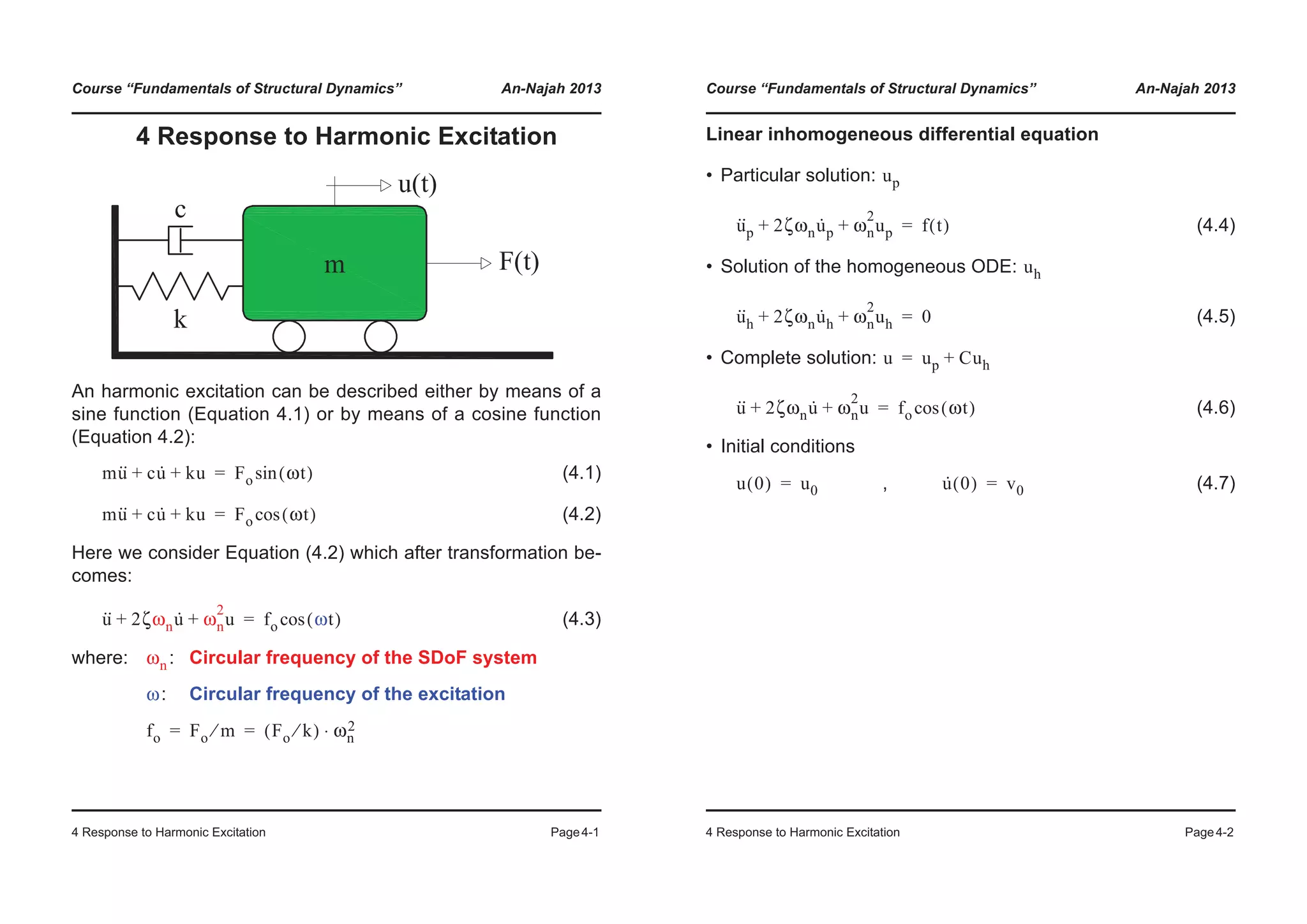
4 Response to Harmonic Excitation Page4-5
4.1.1 Interpretation as a beat
with (4.18)
The solution is:
(4.19)
and using the trigonometric identity
(4.20)
one gets the equation
(4.21)
that describes a beat with:
Fundamental vibration: (4.22)
Envelope: (4.23)
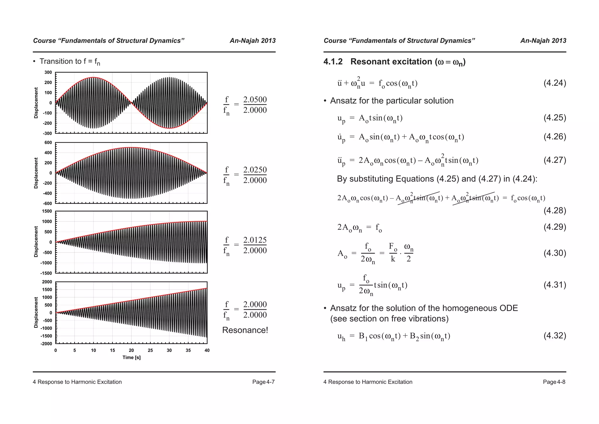
A beat is always present, but is only evident when the natural fre-
quency of the SDoF system and the excitation frequency are
close (see figures on the next page)
u·· ωn
2
u+ fo ωt( )cos= u 0( ) u· 0( ) 0= =
u t( )
fo
ωn
2
ω
2
–
------------------- ωt( )cos ωnt( )cos–[ ]⋅=
α( )cos β( )cos– 2
α β–
2
-------------t
© ¹
§ · α β+
2
-------------t
© ¹
§ ·sinsin–=
u t( )
2fo
ω
2
ωn
2
–
-------------------
ω ωn–
2
----------------t
© ¹
§ · ω ωn+
2
-----------------t
© ¹
§ ·sinsin⋅=
fG
f fn+
2
------------=
fU
f fn–
2
------------=
Course “Fundamentals of Structural Dynamics” An-Najah 2013
4 Response to Harmonic Excitation Page4-6
• Case 1: Natural frequency SDoF 0.2 Hz, excitation frequency 0.4 Hz
• Case 2: Natural frequency SDoF 2.0 Hz, excitation frequency 2.2 Hz
-200
-100
0
100
200
300
400
500
Displacement
Total response Envelope
-500
-400
-300
-200
0 2 4 6 8 10 12 14 16 18 20
Time [s]
-20
0
20
40
60
80
Displacement
Total response Envelope
-80
-60
-40
0 2 4 6 8 10 12 14 16 18 20
Time [s]](https://image.slidesharecdn.com/fundamentalsofstructuraldynamics-200730194708/75/Fundamentals-of-structural-dynamics-30-2048.jpg)
![Course “Fundamentals of Structural Dynamics” An-Najah 2013
4 Response to Harmonic Excitation Page4-9
• Complete solution of the ODE:
(4.33)
By means of the initial conditions given in Equation (4.7), the
constants and can be calculated as follows:
, (4.34)
• Special case
(The homogeneous part of the solution falls away)
(4.35)
Is a sinusoidal vibration with amplitude:
(4.36)
- The amplitude grows linearly with time (see last picture of
interpretation “beat”);
- We have when , i.e. after infinite time the am-
plitude of the vibration is infinite as well.
• Visualization of the solution by means of the Excel file given on
the web page of the course (SD_HE_cosine_viscous.xlsx)
u A1 ωnt( )cos A2 ωnt( )sin
fo
2ωn
----------t ωnt( )sin+ +=
A1 A2
A1 u0= A2
v0
ωn
------=
u0 v0 0= =
u
fo
2ωn
----------t ωnt( )sin=
A
fo
2ωn
----------t=
A ∞→ t ∞→
Course “Fundamentals of Structural Dynamics” An-Najah 2013
4 Response to Harmonic Excitation Page4-10
4.2 Damped harmonic vibration
(4.37)
• Ansatz for particular solution
(4.38)
(4.39)
(4.40)
By substitution Equations (4.38) to (4.40) in (4.37):
(4.41)
Equation (4.41) shall be true for all times and for all
constants and , therefore Equations (4.42) and (4.43)
can be written as follows:
(4.42)
(4.43)
The solution of the system [(4.42), (4.43)] allows the
calculations of the constants and as:
,
(4.44)
u·· 2ζωnu· ωn
2
u+ + fo ωt( )cos=
up A3 ωt( )cos A4 ωt( )sin+=
u·
p A– 3ω ωt( )sin A4ω ωt( )cos+=
u··
p A– 3ω
2
ωt( )cos A4ω
2
ωt( )sin–=
ωn
2
ω
2
–( )A3 2ζωnωA4+[ ] ωt( )cos 2ζωnωA3– ωn
2
ω
2
–( )A4+[ ] ωt( )sin+ fo ωt( )cos=
t
A3 A4
ωn
2
ω
2
–( )A3 2ζωnωA4+ fo=
2ζωnωA3– ωn
2
ω
2
–( )A4+ 0=
A3 A4
A3 fo
ωn
2
ω
2
–
ωn
2
ω
2
–( )
2
2ζωnω( )
2
+
----------------------------------------------------------= A4 fo
2ζωnω
ωn
2
ω
2
–( )
2
2ζωnω( )
2
+
----------------------------------------------------------=](https://image.slidesharecdn.com/fundamentalsofstructuraldynamics-200730194708/75/Fundamentals-of-structural-dynamics-32-2048.jpg)
![Course “Fundamentals of Structural Dynamics” An-Najah 2013
4 Response to Harmonic Excitation Page4-11
• Ansatz for the solution of the homogeneous ODE
(see Section 3.2 on damped free vibrations)
(4.45)
with:
“damped circular frequency” (4.46)
• Complete solution of the ODE:
(4.47)
By means of the initial conditions of Equation (4.7), the con-
stants and can be calculated. The calculation is labo-
rious and should be best carried out with a mathematics pro-
gram (e.g. Maple).
• Denominations:
- Homogeneous part of the solution: “transient”
- Particular part of the solution: “steady-state”
• Visualization of the solution by means of the Excel file given on
the web page of the course (SD_HE_cosine_viscous.xlsx)
uh e
ζωnt–
B1 ωdt( )cos B2 ωdt( )sin+( )=
ωd ωn 1 ζ
2
–=
u e
ζωnt–
A1 ωdt( )cos A2 ωdt( )sin+( ) A3 ωt( )cos A4 ωt( )sin+ +=
A1 A2
Course “Fundamentals of Structural Dynamics” An-Najah 2013
4 Response to Harmonic Excitation Page4-12
• Example 1: fn = 1Hz, f = 0.2Hz, ζ = 5%, fo = 1000, u0 = 0, v0 = fo/ωn
• Example 2: Like 1 but with F(t) = Fosin(ωt) instead of Focos(ωt)
-20
0
20
40
60
Displacement
Steady-state response
Total response
-60
-40
0 2 4 6 8 10 12 14 16 18 20
Time [s]
-20
-10
0
10
20
30
40
50
Displacement
Steady-state response
Total response
-50
-40
-30
20
0 2 4 6 8 10 12 14 16 18 20
Time [s]](https://image.slidesharecdn.com/fundamentalsofstructuraldynamics-200730194708/75/Fundamentals-of-structural-dynamics-33-2048.jpg)
![Course “Fundamentals of Structural Dynamics” An-Najah 2013
4 Response to Harmonic Excitation Page4-15
• Dynamic amplification
• Magnitude of the amplitude after each cycle: f(umax)
20
30
40
50
umax/ust
0
10
0 0.05 0.1 0.15 0.2
Damping ratio ζ [-]
0.4
0.6
0.8
1
abs(uj)/umax
ζ = 0.01
0.02
0.050.1
0.2
0
0.2
0 5 10 15 20 25 30 35 40 45 50
Cycle
Course “Fundamentals of Structural Dynamics” An-Najah 2013
4 Response to Harmonic Excitation Page4-16
• Magnitude of the amplitude after each cycle: f(ust)
20
30
40
50
abs(uj)/ust
ζ = 0.01
0.02
0
10
0 5 10 15 20 25 30 35 40 45 50
Cycle
0.05
0.10
0.20](https://image.slidesharecdn.com/fundamentalsofstructuraldynamics-200730194708/75/Fundamentals-of-structural-dynamics-35-2048.jpg)
![Course “Fundamentals of Structural Dynamics” An-Najah 2013
5 Transfer Functions Page5-1
5 Transfer Functions
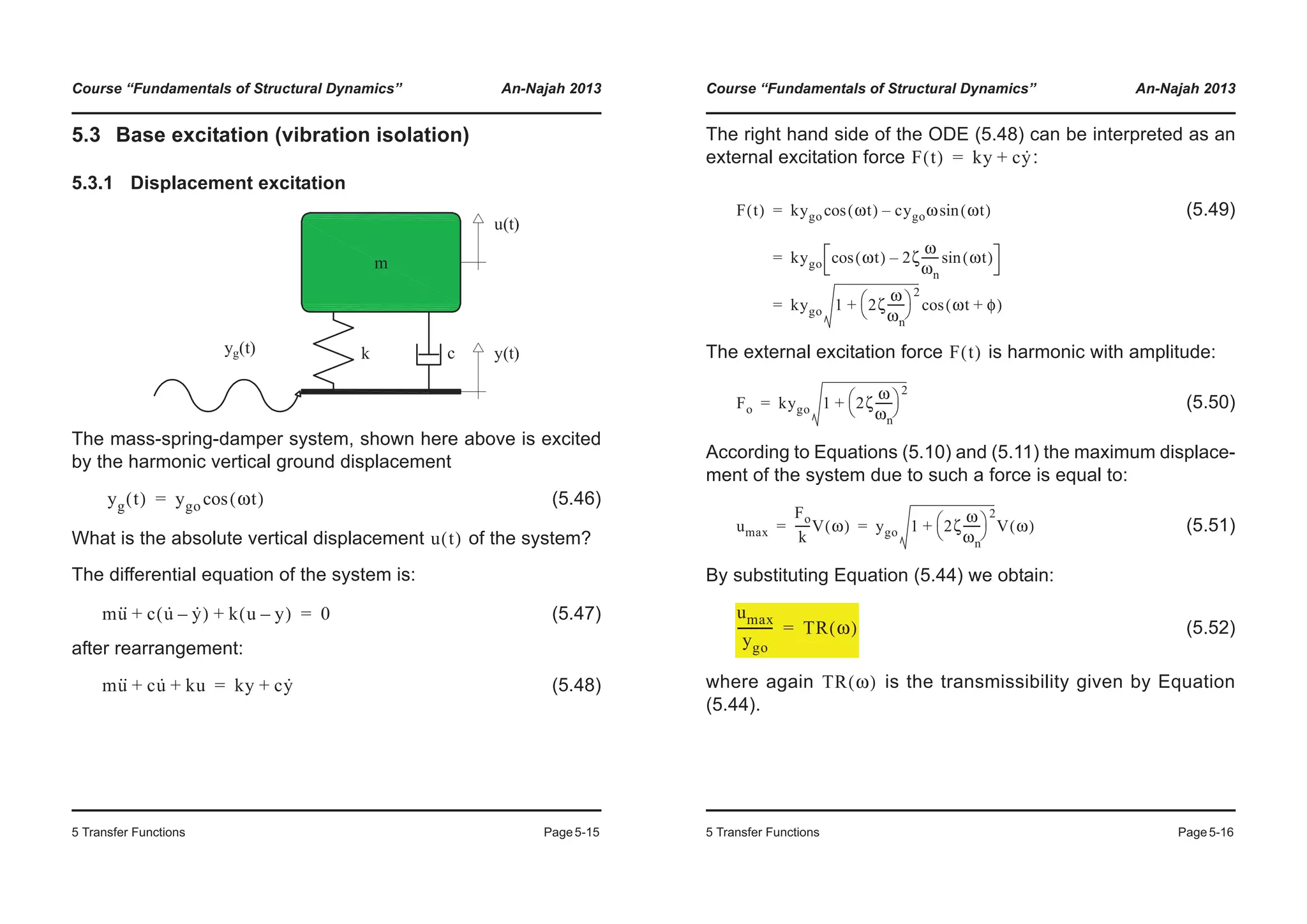
5.1 Force excitation
The steady-state displacement of a system due to harmonic ex-
citation is (see Section 4.2 on harmonic excitation):
(5.1)
with
, (5.2)
By means of the trigonometric identity
where (5.3)
Equation (5.1) can be transformed as follows:
(5.4)
It is a cosine vibration with the maximum dynamic amplitude
:
(5.5)
and the phase angle obtained from:
(5.6)
up a1 ωt( )cos a2 ωt( )sin+=
a1 fo
ωn
2
ω
2
–
ωn
2
ω
2
–( )
2
2ζωnω( )
2
+
----------------------------------------------------------= a2 fo
2ζωnω
ωn
2
ω
2
–( )
2
2ζωnω( )
2
+
----------------------------------------------------------=
a α( )cos b α( )sin+ a
2
b
2
+ α φ–( )cos⋅= φtan
b
a
---=
up umax ωt φ–( )cos=
umax
umax a1
2
a2
2
+=
φ
φtan
a2
a1
-----=
Course “Fundamentals of Structural Dynamics” An-Najah 2013
5 Transfer Functions Page5-2
The maximum dynamic amplitude given by Equation (5.5)
can be transformed to:
(5.7)
(5.8)
(5.9)
(5.10)
Introducing the maximum static amplitude the
dynamic amplification factor can be defined as:
(5.11)
The maximum amplification factor occurs when its deriva-
tive, given by Equation (5.12), is equal to zero.
umax
umax fo
ωn
2
ω
2
–
ωn
2
ω
2
–( )
2
2ζωnω( )
2
+
----------------------------------------------------------
© ¹
¨ ¸
§ ·
2
fo
2ζωnω
ωn
2
ω
2
–( )
2
2ζωnω( )
2
+
----------------------------------------------------------
© ¹
¨ ¸
§ ·2
+=
umax fo
ωn
2
ω
2
–( )
2
2ζωnω( )
2
+
ωn
2
ω
2
–( )
2
2ζωnω( )
2
+[ ]
2
-----------------------------------------------------------------=
umax fo
1
ωn
2
ω
2
–( )
2
2ζωnω( )
2
+
--------------------------------------------------------------=
umax
fo
ωn
2
------
1
1 ω ωn⁄( )
2
–[ ]
2
2ζ ω ωn⁄( )[ ]
2
+
----------------------------------------------------------------------------------=
uo Fo k⁄ fo ωn
2
⁄= =
V ω( )
V ω( )
umax
uo
-----------
1
1 ω ωn⁄( )
2
–[ ]
2
2ζ ω ωn⁄( )[ ]
2
+
-----------------------------------------------------------------------------------= =
V ω( )](https://image.slidesharecdn.com/fundamentalsofstructuraldynamics-200730194708/75/Fundamentals-of-structural-dynamics-36-2048.jpg)
![Course “Fundamentals of Structural Dynamics” An-Najah 2013
5 Transfer Functions Page5-3
(5.12)
when: , (5.13)
The maximum amplification factor occurs when:
for (5.14)
and we have:
: (5.15)
: (5.16)
From Equation (5.6), the phase angle is:
(5.17)
The phase angle has the following interesting property:
(5.18)
at we have: (= when in deg)
(5.19)
ωd
dV 2ωωn
2
ω
2
ωn
2
1 2ζ
2
–( )–[ ]
ω
4
2 1 2ζ
2
–( )ω
2
ωn
2
– ωn
4
+[ ]
3 2⁄( )
---------------------------------------------------------------------------------=
ωd
dV
0= ω 0= ω ωn 1 2ζ
2
–±=
V ω( )
ω ωn 1 2ζ
2
–= ζ
1
2
-------< 0.71≈
ω ωn= V
1
2ζ
------=
ω ωn 1 2ζ
2
–= V
1
2ζ 1 ζ
2
–
-------------------------=
φ
φtan
2ζωnω
ωn
2
ω
2
–
-------------------
2ζ ω ωn⁄( )
1 ω ωn⁄( )
2
–
-------------------------------= =
ω ωn⁄( )d
dφ 2ζ 1 ω ωn⁄( )
2
+[ ]
1 2 ω ωn⁄( )
2
– ω ωn⁄( )
4
4ζ
2
ω ωn⁄( )
2
+ +
----------------------------------------------------------------------------------------------------=
ω ωn⁄ 1=
ω ωn⁄( )d
dφ 1
ζ
---=
1
ζ
---
180
π
---------⋅ φ
Course “Fundamentals of Structural Dynamics” An-Najah 2013
5 Transfer Functions Page5-4
5.1.1 Comments on the amplification factor V
(5.20)
• : Slow variation of the excitation (ζ not important)
• therefore:
• : Motion and excitation force are in phase
• : Quick variation of the excitation (ζ not important)
•
• : Mass controls the behaviour
• : Motion and excitation force are opposite
• : (ζ very important)
•
• : Damping controls the behaviour
• : zero displacement when excitation force is maximum
V ω( )
1
1 ω ωn⁄( )
2
–[ ]
2
2ζ ω ωn⁄( )[ ]
2
+
-----------------------------------------------------------------------------------=
ω ωn⁄ 1«
V ω( ) 1≈ umax uo≈
φ 0≈
ω ωn⁄ 1»
V ω( )
ωn
ω
------
© ¹
§ ·
2
≈
umax uo
ωn
ω
------
© ¹
§ ·
2
⋅≈ Fo mω
2
( )⁄=
φ 180≈
ω ωn⁄( ) 1≈
V ω( )
1
2ζ
------≈
umax uo 2ζ( )⁄≈ Fo cωn( )⁄=
φ 90≈](https://image.slidesharecdn.com/fundamentalsofstructuraldynamics-200730194708/75/Fundamentals-of-structural-dynamics-37-2048.jpg)
![Course “Fundamentals of Structural Dynamics” An-Najah 2013
5 Transfer Functions Page5-5
• Amplification factor
• Phase angle
3
4
5
6
7
8
9
10
lificationfactorV(ω)
0.00
0.10
0.01
ζ = 0.05
0
1
2
3
0 0.5 1 1.5 2
Amp
ω/ωn
0.20
0.50
0.70
90
180
PhaseAngleI
0.00
0.10 0.20 0.50
0.70
0.01
] = 0.05
0
0 0.5 1 1.5 2
Z/Zn
Course “Fundamentals of Structural Dynamics” An-Najah 2013
5 Transfer Functions Page5-6
• Example:
An excitation produces the static displacement
(5.21)
and its maximum is:
(5.22)
The steady-state dynamic response of the system is:
(5.23)
therefore:
, (5.24)
In the next plots the time histories of and are
represented and compared.
The phase angle is always positive and because of the mi-
nus sign in Equation (5.24) it shows how much the response
to the excitation lags behind.
ust
Fo ωt( )cos
k
--------------------------=
uo
Fo
k
-----=
up umax ωt φ–( )cos=
ust
uo
------ ωt( )cos=
up
uo
----- V ωt φ–( )cos=
ust uo⁄ up uo⁄
φ](https://image.slidesharecdn.com/fundamentalsofstructuraldynamics-200730194708/75/Fundamentals-of-structural-dynamics-38-2048.jpg)
![Course “Fundamentals of Structural Dynamics” An-Najah 2013
5 Transfer Functions Page5-7
Frequency of SDoF System fn = 1Hz (ωn = 6.28rad/s), Damping ζ = 0.1
-5
-4
-3
-2
-1
0
1
2
3
4
5
0.00 0.25 0.50 0.75 1.00 1.25 1.50 1.75 2.00
u/uo
Time [s]
Excitation
Steady-state response
-1
0
1
2
3
4
5
u/uo
-5
-4
-3
-2
0.00 0.25 0.50 0.75 1.00 1.25 1.50 1.75 2.00
Time [s]
Excitation
Steady-state response
-5
-4
-3
-2
-1
0
1
2
3
4
5
0.00 0.25 0.50 0.75 1.00 1.25 1.50 1.75 2.00
u/uo
Time [s]
Excitation
Steady-state response
V
Δt
Δt
V
V
Δt
ω ωn⁄ 0.9=
ω 0.9 6.28⋅
5.65 rad/s
=
=
V 3.82=
φ 43.45°
0.76 rad
=
=
Δt
φ
ω
----
0.76
5.65
----------
0.14 s
= =
=
ω ωn⁄ 1.0=
ω 1.0 6.28⋅
6.28 rad/s
=
=
V 5.00=
φ 90.00°
1.57 rad
=
=
Δt
φ
ω
----
1.57
6.28
----------
0.25 s
= =
=
ω ωn⁄ 1.1=
ω 1.1 6.28⋅
6.91 rad/s
=
=
V 3.28=
φ 133.66°
2.33 rad
=
=
Δt
φ
ω
----
2.33
6.91
----------
0.34 s
= =
=
Course “Fundamentals of Structural Dynamics” An-Najah 2013
5 Transfer Functions Page5-8
5.1.2 Steady-state displacement quantities
• Displacement: Corresponds to Equation (5.4)
(5.25)
• Velocity: Obtained by derivating Equation (5.25)
(5.26)
(5.27)
with (5.28)
• Acceleration: Obtained by derivating Equation (5.26)
(5.29)
(5.30)
with (5.31)
up
Fo k⁄
------------ V ω( ) ωt φ–( )cos=
u·
p
Fo k⁄
------------ V ω( )ω ωt φ–( )sin–=
u·
p
Fo k⁄( )ωn
------------------------ V ω( )
ω
ωn
------ ωt φ–( )sin–=
u·
p
Fo km⁄
---------------------- Vv ω( ) ωt φ–( )sin–= Vv ω( )
ω
ωn
------V ω( )=
u··
p
Fo k⁄
------------ V ω( )ω
2
ωt φ–( )cos–=
u··
p
Fo k⁄( )ωn
2
------------------------ V ω( )
ω
2
ωn
2
------ ωt φ–( )cos–=
u··
p
Fo m⁄
-------------- Va ω( ) ωt φ–( )cos–= Va ω( )
ω
2
ωn
2
------V ω( )=](https://image.slidesharecdn.com/fundamentalsofstructuraldynamics-200730194708/75/Fundamentals-of-structural-dynamics-39-2048.jpg)
![Course “Fundamentals of Structural Dynamics” An-Najah 2013
5 Transfer Functions Page5-9
• Amplification factors
Resonant
displacement
Resonant
velocity
Resonant
acceleration
0
1
2
3
4
5
6
7
8
9
10
0 0.5 1 1.5 2
AmplificationFactorV(ω)
ω/ωn
0.00
0.10
0.20
0.50
0.70
0.01
ζ = 0.05
4
5
6
7
8
9
10
cationfactorVv(ω)
0.00
0 10
0.01
ζ = 0.05
0
1
2
3
4
0 0.5 1 1.5 2
Amplificati
ω/ωn
0.10
0.20
0.50
0.70
0
1
2
3
4
5
6
7
8
9
10
0 0.5 1 1.5 2
AmplificationfactorVa(ω)
ω/ωn
0.00
0.10
0.20
0.50
0.70
0.01
ζ = 0.05
ω ωn 1 2ζ
2
–=
V
1
2ζ 1 ζ–
----------------------=
ω ωn=
V
1
2ζ
------=
ω
ωn
1 2ζ
2
–
----------------------=
V
1
2ζ 1 ζ–
----------------------=
Course “Fundamentals of Structural Dynamics” An-Najah 2013
5 Transfer Functions Page5-10
5.1.3 Derivating properties of SDoF systems from
harmonic vibrations
• Half-power bandwidth
Condition:
(5.32)
(5.33)
(5.34)
(5.35)
3
4
5
6
7
8
9
10
plificationfactorV(ω)
0
1
2
3
0 0.5 1 1.5 2
Amp
ω/ωn
ζ = 0.05
V(Resonance)
V(Resonance)
2
2ζ
ωa ωb
V ω( )
V ω ωn⁄ 1 2ζ
2
–=( )
2
-----------------------------------------------------
1
2
-------
1
2ζ 1 ζ–
----------------------⋅= =
1
1 ω ωn⁄( )
2
–[ ]
2
2ζ ω ωn⁄( )[ ]
2
+
----------------------------------------------------------------------------------
1
2
-------
1
2ζ 1 ζ–
----------------------⋅=
ω
ωn
------
© ¹
§ ·4
2 1 2ζ
2
–( )
ω
ωn
------
© ¹
§ ·2
– 1 8ζ
2
1 ζ
2
–( )–+ 0=
ω
ωn
------
© ¹
§ ·2
1 2ζ
2
– 2ζ 1 ζ
2
–±=](https://image.slidesharecdn.com/fundamentalsofstructuraldynamics-200730194708/75/Fundamentals-of-structural-dynamics-40-2048.jpg)
![Course “Fundamentals of Structural Dynamics” An-Najah 2013
5 Transfer Functions Page5-11
For small damping, the terms featuring can be neglected:
(5.36)
This yield the solution for the half-power bandwidth:
(5.37)
• Remarks on the frequency response curve
• The natural frequency of the system can be derived from the res-
onant response. However, it is sometimes problematic to build the
whole frequency response curve because at resonance the sys-
tem could be damaged. For this reason it is often better to deter-
mine the properties of a system based on vibration decay tests
(see section on free vibration)
• The natural frequency can be estimated by varying the Excita-
tion until a phase shift in the response occurs.
• Damping can be calculated by means of Equation (5.15) as:
However, it is sometimes difficult to determine the static deflection
, therefore, the definition of half-power bandwidth is used to
estimate the damping.
• Damping can be determined from the slope of the phase angle
curve using Equation (5.19).
ζ
2
ω
ωn
------ 1 2ζ± 1 ζ±≈ ≈
2ζ
ωb ωa–
ωn
-------------------=
ωn
90°
ζ
1
2
---
uo
umax
-----------⋅=
uo
Course “Fundamentals of Structural Dynamics” An-Najah 2013
5 Transfer Functions Page5-12
5.2 Force transmission (vibration isolation)
The reaction force results from the sum of the spring force
and the damper’s force
(5.38)
The steady-state deformation of the system due to harmonic ex-
citation is according to Equation (5.4):
with (5.39)
By substituting Equation (5.39) and its derivative into Equation
(5.38) we obtain:
(5.40)
The mass-spring-damper system,
shown here on the right, is excited
by the harmonic force
What is the reaction force ,
which is introduced in the founda-
tion?
F t( ) Fo ωt( )cos=
FT t( )
FT t( )
Fs Fc
FT t( ) Fs t( ) Fc t( )+ ku t( ) cu· t( )+= =
F t( )
up umax ωt φ–( )cos= umax uoV ω( )
Fo
k
-----V ω( )= =
FT t( )
Fo
k
-----V ω( ) k ωt φ–( )cos cω ωt φ–( )sin–[ ]=](https://image.slidesharecdn.com/fundamentalsofstructuraldynamics-200730194708/75/Fundamentals-of-structural-dynamics-41-2048.jpg)
![Course “Fundamentals of Structural Dynamics” An-Najah 2013
5 Transfer Functions Page5-13
with the trigonometric identity from Equation (5.3):
(5.41)
and by substituting the identity :
(5.42)
the maximum reaction force becomes:
(5.43)
where the quantity is called Transmissibility and it is
equal to:
(5.44)
Special case:
(5.45)
FT t( )
Fo
k
-----V ω( ) k
2
c
2
ω
2
+ ωt φ–( )cos[ ]=
c 2ζk( ) ωn⁄=
FT t( ) FoV ω( ) 1 2ζ
ω
ωn
------
© ¹
§ ·2
+ ωt φ–( )cos=
FT,max
Fo
--------------- TR ω( )=
TR ω( )
TR ω( ) V ω( ) 1 2ζ
ω
ωn
------
© ¹
§ ·2
+
1 2ζ ω ωn⁄( )[ ]
2
+
1 ω ωn⁄( )
2
–[ ]
2
2ζ ω ωn⁄( )[ ]
2
+
------------------------------------------------------------------------------
=
=
TR
ω
ωn
------ 1=
© ¹
§ · 1 4ζ
2
+
2ζ
----------------------=
Course “Fundamentals of Structural Dynamics” An-Najah 2013
5 Transfer Functions Page5-14
• Representation of the transmissibility TR
- When then : Vibration isolation
- When damping has a stiffening effect
- High tuning (sub-critical excitation)
- Low tuning (super-critical excitation):
Pay attention to the starting phase!
3
4
5
6
7
8
9
10
rasmissibilityTR
0.00
0.10
0.01
ζ = 0.05
0
1
2
3
0 0.5 1 1.5 2 2.5 3 3.5 4
Tr
ω/ωn
0.20
0.50
0.70 2
ω ωn⁄ 2> TR 1<
ω ωn⁄ 2>](https://image.slidesharecdn.com/fundamentalsofstructuraldynamics-200730194708/75/Fundamentals-of-structural-dynamics-42-2048.jpg)
![Course “Fundamentals of Structural Dynamics” An-Najah 2013
5 Transfer Functions Page5-21
• Case 1: Initial situation with ζ = 2%
0 10 20 30 40 50 60 70 80 90 100
0
1
2
Excitationfreq.[Hz]
0 10 20 30 40 50 60 70 80 90 100
0
5
10
Excitationamplitude[m/s2
]
0 10 20 30 40 50 60 70 80 90 100
-10
-5
0
5
10
Excitation[m/s2
]
0 10 20 30 40 50 60 70 80 90 100
Time [s]
-20
-10
0
10
20
Aabs
SDoF[m/s2
]
f=fn=0.5Hz
Course “Fundamentals of Structural Dynamics” An-Najah 2013
5 Transfer Functions Page5-22
• Case 2: Increase of the damping rate from ζ = 2% to ζ = 20%
0 10 20 30 40 50 60 70 80 90 100
0
1
2
Excitationfreq.[Hz]
0 10 20 30 40 50 60 70 80 90 100
0
5
10
Excitationamplitude[m/s2
]
0 10 20 30 40 50 60 70 80 90 100
-10
-5
0
5
10
Excitation[m/s2
]
0 10 20 30 40 50 60 70 80 90 100
Time [s]
-20
-10
0
10
20
Aabs
SDoF[m/s2
]
f=fn=0.5Hz](https://image.slidesharecdn.com/fundamentalsofstructuraldynamics-200730194708/75/Fundamentals-of-structural-dynamics-46-2048.jpg)
![Course “Fundamentals of Structural Dynamics” An-Najah 2013
5 Transfer Functions Page5-23
• Case 3: Reduction of starting time from ta = 80s to ta = 20s (ζ = 2%)
0 10 20 30 40 50 60 70 80 90 100
0
1
2
Excitationfreq.[Hz]
0 10 20 30 40 50 60 70 80 90 100
0
5
10
Excitationamplitude[m/s2
]
0 10 20 30 40 50 60 70 80 90 100
-10
-5
0
5
10
Excitation[m/s2
]
0 10 20 30 40 50 60 70 80 90 100
Time [s]
-20
-10
0
10
20
Aabs
SDoF[m/s2
]
f=fn=0.5Hz
Course “Fundamentals of Structural Dynamics” An-Najah 2013
5 Transfer Functions Page5-24
• Case 4: Change the start function for the amplitude (ζ = 2%)
0 10 20 30 40 50 60 70 80 90 100
0
1
2
Excitationfreq.[Hz]
0 10 20 30 40 50 60 70 80 90 100
0
5
10
Excitationamplitude[m/s2
]
0 10 20 30 40 50 60 70 80 90 100
-10
-5
0
5
10
Excitation[m/s2
]
0 10 20 30 40 50 60 70 80 90 100
Time [s]
-20
-10
0
10
20
Aabs
SDoF[m/s2
]
f=fn=0.5Hz](https://image.slidesharecdn.com/fundamentalsofstructuraldynamics-200730194708/75/Fundamentals-of-structural-dynamics-47-2048.jpg)
![Course “Fundamentals of Structural Dynamics” An-Najah 2013
5 Transfer Functions Page5-25
• Notes
The excitation function in the starting phase has the form:
(5.66)
The excitation angular frequency varies with time, and is:
(5.67)
• Linear variation of the excitation circular frequency
: (5.68)
• Parabolic variation of the excitation circular frequency
: (5.69)
• Sinusoidal variation of the excitation circular frequency
:
(5.70)
• Double-sinusoidal variation of the excitation circular frequency
: (5.71)
• Visualization of the solution by means of the Excel file given on
the web page of the course (SD_HE_Starting_Phase.xlsx)
y··
g t( ) A t( ) Ω t( ) t⋅( )cos=
ω t( )
td
d
Ω t( ) t⋅( )=
Ω t( )
ω0
2ta
------- t⋅= ω t( ) ω0
t
ta
---⋅= 0 t ta≤ ≤( )
Ω t( )
ω0
3ta
2
------- t
2
⋅= ω t( ) ω0
t
ta
---
© ¹
§ ·2
⋅= 0 t ta≤ ≤( )
Ω t( )
2ω0ta
πt
-------------- π
2
---
t
ta
---⋅
© ¹
§ ·cos–= ω t( ) ω0
π
2
---
t
ta
---⋅
© ¹
§ ·sin⋅= 0 t ta≤ ≤( )
Ω t( )
ω0
2
------ 1
π
t
ta
---⋅
© ¹
§ · tasin
πt
-----------------------------–= ω t( ) ω0 1 π
t
ta
---⋅
© ¹
§ ·cos–=
Course “Fundamentals of Structural Dynamics” An-Najah 2013
5 Transfer Functions Page5-26
5.4 Summary Transfer Functions
(5.72)
(5.73)
• Force excitation:
• Force transmission:
• Displacement excitation:
• Acceleration excitation
• For further cases check the literature.
V ω( )
1
1 ω ωn⁄( )
2
–[ ]
2
2ζ ω ωn⁄( )[ ]
2
+
-----------------------------------------------------------------------------------=
TR ω( )
1 2ζ ω ωn⁄( )[ ]
2
+
1 ω ωn⁄( )
2
–[ ]
2
2ζ ω ωn⁄( )[ ]
2
+
------------------------------------------------------------------------------=
umax
uo
----------- V ω( )=
FT,max
Fo
--------------- TR ω( )=
umax
ygo
----------- TR ω( )=
u··
max
y··
go
----------- TR ω( )=
urel max,
y··
go ωn
2
⁄( )
----------------------- V ω( )=](https://image.slidesharecdn.com/fundamentalsofstructuraldynamics-200730194708/75/Fundamentals-of-structural-dynamics-48-2048.jpg)
![Course “Fundamentals of Structural Dynamics” An-Najah 2013
6 Forced Vibrations Page6-1
6 Forced Vibrations
6.1 Periodic excitation
An excitation is periodic if:
for (6.1)
The function can be represented as a sum of several har-
monic functions in the form of a Fourier series, namely:
(6.2)
1.5
2.0
2.5
3.0
3.5
4.0
ForceF(t)[kN]
Half-sine excitation
0.0
0.5
1.0
0 0.1 0.2 0.3 0.4 0.5 0.6 0.7 0.8 0.9 1
F
Time (s)
T0
F t nT0+( ) F t( )= n ∞– … 1– 0 1 … ∞, , , , , ,=
F t( )
F t( ) a0
an nω0t( )cos bn nω0t( )sin+[ ]
n 1=
∞
¦+=
Course “Fundamentals of Structural Dynamics” An-Najah 2013
6 Forced Vibrations Page6-2
with the fundamental frequency
(6.3)
Taking into account the orthogonality relations:
(6.4)
(6.5)
(6.6)
the Fourier coefficients can be computed by multiplying Equation
(6.2) by first, and then integrating it over the period .
•
(6.7)
(6.8)
(6.9)
ω0
2π
T0
------=
nω0t( ) jω0t( )sinsin td
0
T0
³
0 for n j≠
T0 2⁄ for n j=¯
®
=
nω0t( )cos jω0t( )cos td
0
T0
³
0 for n j≠
T0 2⁄ for n j=¯
®
=
nω0t( )cos jω0t( )sin td
0
T0
³ 0=
an
jω0t( )cos T0
j 0=
F t( ) jω0t( )cos td
0
T0
³ a0 jω0t( )cos td
0
T0
³
an nω0t( )cos jω0t( )cos td
0
T0
³ bn nω0t( )sin jω0t( )cos td
0
T0
³+
n 1=
∞
¦+
=
F t( ) td
0
T0
³ a0 td
0
T0
³ a0T0= =
a0
1
T0
------ F t( ) td
0
T0
³⋅=](https://image.slidesharecdn.com/fundamentalsofstructuraldynamics-200730194708/75/Fundamentals-of-structural-dynamics-49-2048.jpg)
![Course “Fundamentals of Structural Dynamics” An-Najah 2013
6 Forced Vibrations Page6-3
•
(6.10)
(6.11)
(6.12)
Similarly, the Fourier coefficients can be computed by first
multiplying Equation (6.2) by and then integrating it
over the period .
(6.13)
• Notes
- is the mean value of the function
- The integrals can also be calculated over the interval
- For no b-coefficient exists
j n=
F t( ) jω0t( )cos td
0
T0
³ a0 jω0t( )cos td
0
T0
³
an nω0t( )cos jω0t( )cos td
0
T0
³ bn nω0t( )sin jω0t( )cos td
0
T0
³+
n 1=
∞
¦+
=
F t( ) nω0t( )cos td
0
T0
³ an
T0
2
-----⋅=
an
2
T0
------ F t( ) nω0t( )cos td
0
T0
³⋅=
bn
jω0t( )sin
T0
bn
2
T0
------ F t( ) nω0t( )sin td
0
T0
³⋅=
a0 F t( )
T0 2⁄– T0 2⁄[ , ]
j 0=
Course “Fundamentals of Structural Dynamics” An-Najah 2013
6 Forced Vibrations Page6-4
6.1.1 Steady state response due to periodic excitation
(6.14)
(6.15)
(6.16)
• Static Part ( )
(6.17)
• Harmonic part “cosine” (see harmonic excitation)
,
(6.18)
• Harmonic part “sine” (similar as “cosine”)
,
(6.19)
• The steady-state response of a damped SDoF system un-
der the periodic excitation force is equal to the sum of the
terms of the Fourier series.
(6.20)
mu·· cu· ku+ + F t( )=
u·· 2ζωnu· ωn
2
u+ +
F t( )
m
----------=
F t( ) a0 an nω0t( )cos bn nω0t( )sin+[ ]
n 1=
∞
¦+=
a0
u0 t( )
a0
k
-----=
un
Co esin
t( )
an
k
-----
2ζβn nω0t( )sin 1 βn
2
–( ) nω0t( )cos+
1 βn
2
–( )
2
2ζβn( )
2
+
-----------------------------------------------------------------------------------------⋅= βn
nω0
ωn
---------=
un
Sine
t( )
bn
k
-----
1 βn
2
–( ) nω0t( )sin 2ζβn nω0t( )cos–
1 βn
2
–( )
2
2ζβn( )
2
+
-----------------------------------------------------------------------------------------⋅= βn
nω0
ωn
---------=
u t( )
F t( )
u t( ) u0 t( ) un
Co esin
t( )
n 1=
∞
¦ un
Sine
t( )
n 1=
∞
¦+ +=](https://image.slidesharecdn.com/fundamentalsofstructuraldynamics-200730194708/75/Fundamentals-of-structural-dynamics-50-2048.jpg)
![Course “Fundamentals of Structural Dynamics” An-Najah 2013
6 Forced Vibrations Page6-5
6.1.2 Half-sine
A series of half-sine functions is a good model for the force that
is generated by a person jumping.
(6.21)
The Fourier coefficients can be calculated at the best using a
mathematics program:
with (6.22)
1.5
2.0
2.5
3.0
3.5
4.0
ForceF(t)[kN]
Half-sine excitation
0.0
0.5
1.0
0 0.1 0.2 0.3 0.4 0.5 0.6 0.7 0.8 0.9 1
F
Time (s)
T0
tp
F t( )
A
πt
tp
-----
© ¹
§ · for 0 t tp<≤sin
0 for tp t T0<≤¯
°
®
°
=
a0
A
T0
------
πt
tp
-----
© ¹
§ ·sin td
0
tp
³⋅
2Aτ
π
----------= = τ
tp
T0
------=
Course “Fundamentals of Structural Dynamics” An-Najah 2013
6 Forced Vibrations Page6-6
(6.23)
(6.24)
The approximation of the half-sine model for and
by means of 6 Fourier terms is as follows:
• Note
The static term corresponds to the weight of
the person jumping.
an
2A
T0
-------
πt
tp
-----
© ¹
§ ·sin nω0t( ) tdcos
0
tp
³⋅
4Aτ nπτ( )cos
2
π 1 4n
2
τ
2
–( )
-------------------------------------= =
bn
2A
T0
-------
πt
tp
-----
© ¹
§ ·sin nω0t( ) tdsin
0
tp
³⋅
4Aτ nπτ( )sin nπτ( )cos
π 1 4n
2
τ
2
–( )
---------------------------------------------------------= =
T0 0.5s=
tp 0.16s=
0.0
1.0
2.0
3.0
4.0
ForceF(t)[kN]
Static term (n=0)
First harmonic (n=1)
Second harmonic (n=2)
Third harmonic (n=3)
Total (6 harmonics)
-2.0
-1.0
0 0.1 0.2 0.3 0.4 0.5 0.6 0.7 0.8 0.9 1
F
Time (s)
T0
a0 2Aτ π⁄ G= =](https://image.slidesharecdn.com/fundamentalsofstructuraldynamics-200730194708/75/Fundamentals-of-structural-dynamics-51-2048.jpg)
![Course “Fundamentals of Structural Dynamics” An-Najah 2013
6 Forced Vibrations Page6-7
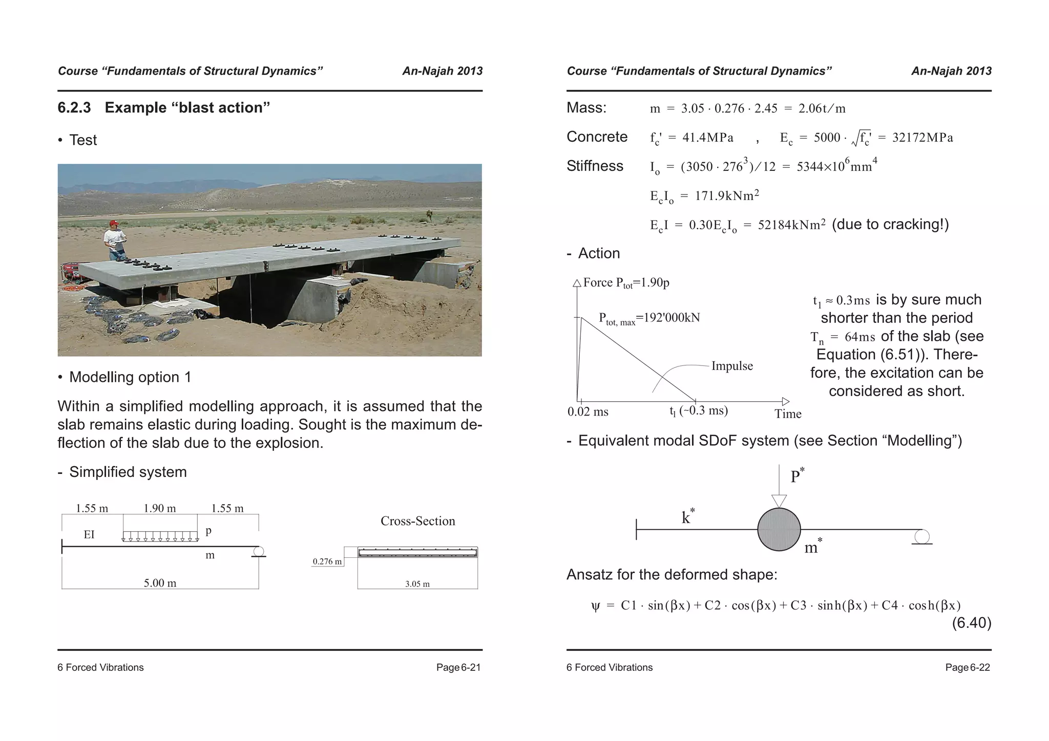
6.1.3 Example: “Jumping on a reinforced concrete beam”
• Beam
• Excitation (similar to page 186 of [Bac+97])
• Young’s Modulus:
• Density:
• Bending stiffness:
• Damping rate
• Modal mass
• Modal stiffness
• Jumping frequency:
• Period:
• Contact time:
• Person’s weight:
• Amplitude:
E 23500MPa=
ρ 20.6kN m3⁄=
EI 124741kNm2=
ζ 0.017=
Mn 0.5Mtot=
Kn
π4
2
----- EI
L3
------⋅=
1.5
2.0
2.5
3.0
3.5
4.0
ForceF(t)[kN]
Half-sine excitation
0.0
0.5
1.0
0 0.1 0.2 0.3 0.4 0.5 0.6 0.7 0.8 0.9 1
F
Time (s)
f0 2Hz=
T0 0.5s=
tp 0.16s=
G 0.70kN=
A 3.44kN=
Course “Fundamentals of Structural Dynamics” An-Najah 2013
6 Forced Vibrations Page6-8
• Maximum deflections
Static:
Dynamic: with from Equation (6.20)
Ratio:
• Investigated cases
• Notes
- When the excitation frequency is twice as large as the
natural frequency of the beam, the magnification factor
is small.
- Taking into account the higher harmonics can be impor-
tant!
Length
[m]
Frequency fn
[Hz]
umax
[m] [-]
26.80 1 0.003 1.37
19.00 2 0.044 55.94
15.50 3 0.002 3.62
13.42 4 0.012 41.61
12.01 5 0.001 4.20
10.96 6 0.004 25.02
ust
G
Kn
------=
umax max u t( )( )= u t( )
V
umax
ust
-----------=
V
f0
fn
V](https://image.slidesharecdn.com/fundamentalsofstructuraldynamics-200730194708/75/Fundamentals-of-structural-dynamics-52-2048.jpg)
![Course “Fundamentals of Structural Dynamics” An-Najah 2013
6 Forced Vibrations Page6-9
• Case1: f0 = 2Hz, fn = 1Hz
• Case 2: f0 = 2Hz, fn = 2Hz
0 0000
0.0005
0.0010
0.0015
0.0020
0.0025
0.0030
0.0035
Displacement[m]
Static term (n=0)
First harmonic (n=1)
Second harmonic (n=2)
Third harmonic (n=3)
Total (6 harmonics)
-0.0015
-0.0010
-0.0005
0.0000
0 0.1 0.2 0.3 0.4 0.5 0.6 0.7 0.8 0.9 1
D
Time (s)
0 0200
-0.0100
0.0000
0.0100
0.0200
0.0300
0.0400
0.0500
Displacement[m]
-0.0500
-0.0400
-0.0300
-0.0200
0 0.1 0.2 0.3 0.4 0.5 0.6 0.7 0.8 0.9 1
D
Time (s)
Static term (n=0)
First harmonic (n=1)
Second harmonic (n=2)
Third harmonic (n=3)
Total (6 harmonics)
Course “Fundamentals of Structural Dynamics” An-Najah 2013
6 Forced Vibrations Page6-10
• Case 3: f0 = 2Hz, fn = 3Hz
• Case 4: f0 = 2Hz, fn = 4Hz
0.0000
0.0005
0.0010
0.0015
0.0020
Displacement[m]
Static term (n=0)
First harmonic (n=1)
Second harmonic (n=2)
Third harmonic (n=3)
Total (6 harmonics)
-0.0010
-0.0005
0 0.1 0.2 0.3 0.4 0.5 0.6 0.7 0.8 0.9 1
D
Time (s)
-0.0050
0.0000
0.0050
0.0100
0.0150
Displacement[m]
Static term (n=0)
First harmonic (n=1)
Second harmonic (n=2)
Third harmonic (n=3)
Total (6 harmonics)
-0.0150
-0.0100
0 0.1 0.2 0.3 0.4 0.5 0.6 0.7 0.8 0.9 1
D
Time (s)](https://image.slidesharecdn.com/fundamentalsofstructuraldynamics-200730194708/75/Fundamentals-of-structural-dynamics-53-2048.jpg)
![Course “Fundamentals of Structural Dynamics” An-Najah 2013
6 Forced Vibrations Page6-11
• Case 5: f0 = 2Hz, fn = 5Hz
• Case 6: f0 = 2Hz, fn = 6Hz
-0.0002
0.0000
0.0002
0.0004
0.0006
0.0008
0.0010
Displacement[m]
Static term (n=0)
First harmonic (n=1)
Second harmonic (n=2)
Third harmonic (n=3)
Total (6 harmonics)
-0.0008
-0.0006
-0.0004
0 0.1 0.2 0.3 0.4 0.5 0.6 0.7 0.8 0.9 1
D
Time (s)
-0.0010
0.0000
0.0010
0.0020
0.0030
0.0040
0.0050
Displacement[m]
Static term (n=0)
First harmonic (n=1)
Second harmonic (n=2)
Third harmonic (n=3)
Total (6 harmonics)
-0.0040
-0.0030
-0.0020
0 0.1 0.2 0.3 0.4 0.5 0.6 0.7 0.8 0.9 1
D
Time (s)
Course “Fundamentals of Structural Dynamics” An-Najah 2013
6 Forced Vibrations Page6-12
6.2 Short excitation
6.2.1 Step force
The differential equation of an undamped SDoF System loaded
with a force which is applied suddenly at the time is:
(6.25)
There is a homogeneous and a particular solution
(see free vibrations) (6.26)
(6.27)
The overall solution is completely defined by the in-
itial conditions and it is:
(6.28)
• Notes
• The damped case can be solved in the exact same way. On the
web page of the course there is an Excel file to illustrate this exci-
tation.
• The maximum displacement of an undamped SDoF System under
a step force is twice the static deflection .
• The deflection at the time of a damped SDoF System under
a step force is equal to the static deflection .
F0 t 0=
mu·· ku+ F0=
uh A1 ωnt( )cos A2 ωnt( )sin+=
up F0 k⁄=
u t( ) uh up+=
u 0( ) u· 0( ) 0= =
u t( )
F0
k
----- 1 ωnt( )cos–[ ]=
ust F0 k⁄=
t ∞=
ust F0 k⁄=](https://image.slidesharecdn.com/fundamentalsofstructuraldynamics-200730194708/75/Fundamentals-of-structural-dynamics-54-2048.jpg)
![Course “Fundamentals of Structural Dynamics” An-Najah 2013
6 Forced Vibrations Page6-13
• Step force: Tn=2s, Fo/k=2, ζ=0
• Step force: Tn=2s, Fo/k=2, ζ=10%
1.5
2
2.5
3
3.5
4
4.5
Displacement
Dynamic response
Excitation
0
0.5
1
0 1 2 3 4 5 6 7 8 9 10
Time (s)
1.5
2
2.5
3
3.5
4
Displacement
Dynamic response
Excitation
0
0.5
1
0 1 2 3 4 5 6 7 8 9 10
Time (s)
Course “Fundamentals of Structural Dynamics” An-Najah 2013
6 Forced Vibrations Page6-14
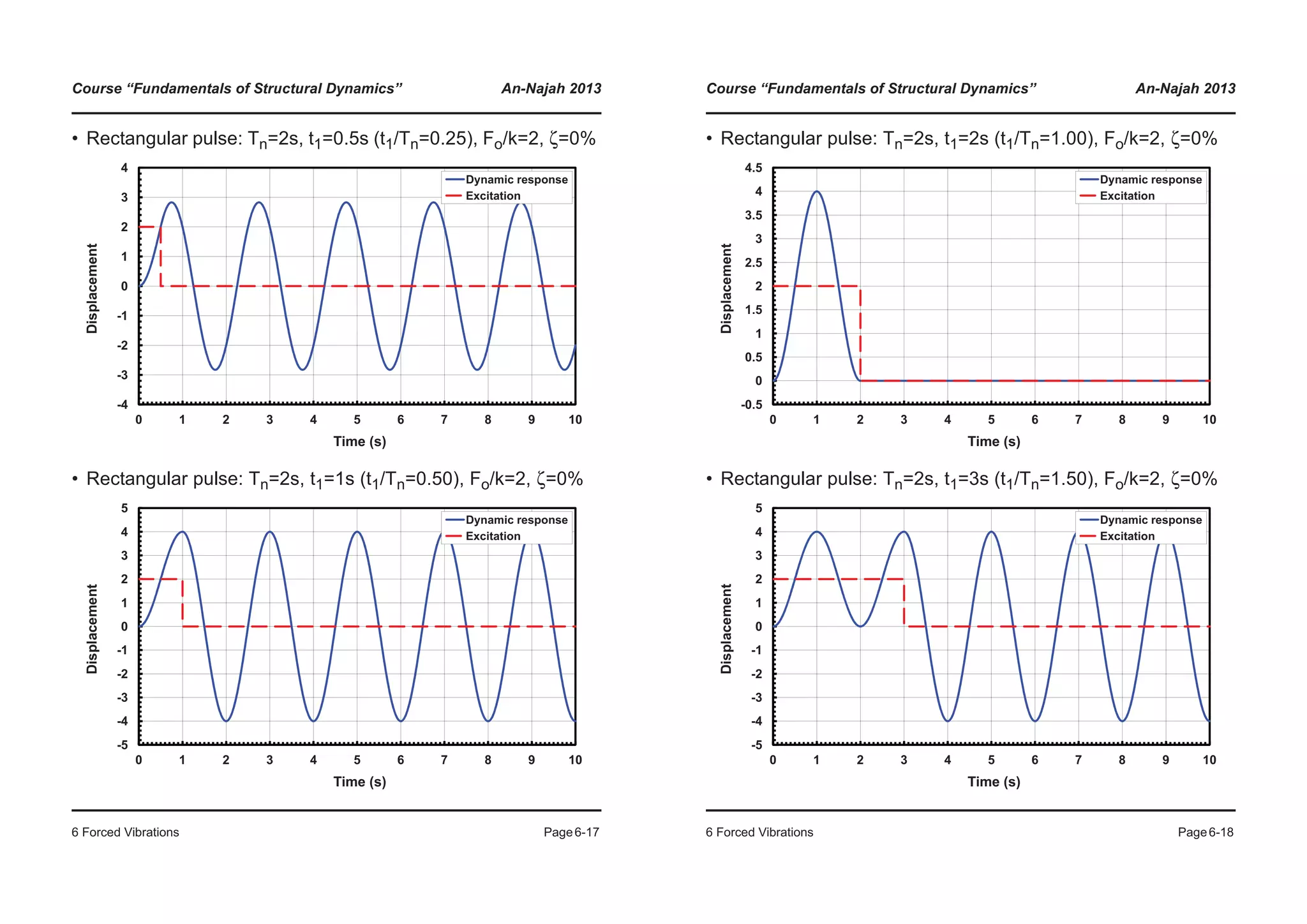
6.2.2 Rectangular pulse force excitation
The differential equation of an undamped SDoF system under a
rectangular pulse force excitation is:
(6.29)
Up to time the solution of the ODE corresponds to Equa-
tion (6.28). From time onwards, it is a free vibration with
the following initial conditions:
(6.30)
(6.31)
The free vibration is described by the following equation:
(6.32)
and through the initial conditions (6.30) and (6.31), the constants
and can be determined.
mu·· ku+ F0 for t t1≤=
mu·· ku+ 0 for t t1>=¯
®
t t1=
t t1=
u t1( )
F0
k
----- 1 ωnt1( )cos–[ ]=
u· t1( )
F0
k
-----ωn ωnt1( )sin=
uh A1 ωn t t1–( )( )cos A2 ωn t t1–( )( )cos+=
A1 A2](https://image.slidesharecdn.com/fundamentalsofstructuraldynamics-200730194708/75/Fundamentals-of-structural-dynamics-55-2048.jpg)
![Course “Fundamentals of Structural Dynamics” An-Najah 2013
6 Forced Vibrations Page6-23
Boundary conditions:
, , , (6.41)
By means of the mathematics program “Maple” Equation (6.40)
can be solved for the boundary conditions (6.41) and we get:
(6.42)
with
(6.43)
The shape of the function is:
And with the equations given in Section “Modelling”, the modal
properties of the equivalent SDoF system are determined:
(6.44)
ψ 0( ) 0= ψ L( ) 0= ψ' 0( ) 0= ψ'' L( ) 0=
1.508 ψ⋅ βx( )sin h βx( )sin–
βL( )sin h βL( )sin+[ ] βx( )cos h βx( )cos–[ ]⋅
βL( )cos– h βL( )cos–
------------------------------------------------------------------------------------------------------------------+=
βL 3.927=
ψ
0
0.2
0.4
0.6
0.8
1
0 0.1 0.2 0.3 0.4 0.5 0.6 0.7 0.8 0.9 1
x/L [-]
[-]
m* m ψ
2
xd⋅ ⋅
0
L
³ 0.439mL= =
Course “Fundamentals of Structural Dynamics” An-Najah 2013
6 Forced Vibrations Page6-24
(6.45)
(6.46)
For this example, the modal properties characterizing the equiv-
alent modal SDoF system are:
(6.47)
(6.48)
(6.49)
(6.50)
(6.51)
The maximum elastic deformation of the SDoF system can be
calculated using the modal pulse as follows:
(6.52)
The initial velocity of the free vibration is:
(6.53)
The maximum elastic deflection is:
(6.54)
k* EI ψ''( )
2
xd⋅ ⋅( )
0
L
³ 104.37
EI
L3
------⋅= =
P* p ψ xd⋅ ⋅( )
L1=1.55m
L2=3.45m
³ 0.888 Ptot⋅= =
m* 0.439 2.06 5⋅ ⋅ 4.52t= =
k* 104.37
52184
53
---------------⋅ 43571kN/m= =
P* 0.888 192000⋅ 170496kN= =
ω k* m*⁄ 43571 4.52⁄ 98.18rad/s= = =
Tn 2π ω⁄ 0.064s= =
I* 0.5 P* t0⋅ ⋅ 0.5 170496 0.3
3–
×10⋅ ⋅ 25.6kNs= = =
v0
I*
m*
-------
25.6
4.52
---------- 5.66m/s= = =
Δm e, v0 ω⁄ 5.66 98.18⁄ 0.058m= = =](https://image.slidesharecdn.com/fundamentalsofstructuraldynamics-200730194708/75/Fundamentals-of-structural-dynamics-60-2048.jpg)
![Course “Fundamentals of Structural Dynamics” An-Najah 2013
6 Forced Vibrations Page6-25
• Modelling option 2
Within a simplified modelling approach, it is assumed that the
slab remains elastic during loading. Sought is the maximum de-
flection of the slab due to the explosion.
- Simplified system
- Equivalent modal SDoF system (see Section “Modelling”)
Ansatz for the deformed shape:
(6.55)
Boundary conditions:
, , , (6.56)
The shape of the function is:
ψ
2πx
L
----------
© ¹
§ ·sin–=
ψ 0( ) 0= ψ L( ) 0= ψ'' 0( ) 0= ψ'' L( ) 0=
ψ
Course “Fundamentals of Structural Dynamics” An-Najah 2013
6 Forced Vibrations Page6-26
And with the equations given in Section “Modelling”, the modal
properties of the equivalent SDoF system are determined:
(6.57)
(6.58)
(6.59)
For this example, the modal properties characterizing the equiv-
alent modal SDoF system are:
(6.60)
(6.61)
(6.62)
(6.63)
-1
-0.8
-0.6
-0.4
-0.2
0
0.2
0.4
0.6
0.8
1
0 0.1 0.2 0.3 0.4 0.5 0.6 0.7 0.8 0.9 1
x/L [-]
ψ[-]
m* m ψ
2
xd⋅ ⋅
0
L
³ 0.5mL= =
k* EI ψ''( )
2
xd⋅ ⋅( )
0
L
³ 8π
4 EI
L3
------⋅ 779.27
EI
L3
------⋅= = =
P* p ψ xd⋅ ⋅( )
L1=6.55m
L2=8.45m
³ 0.941 Ptot⋅= =
m* 0.5 2.06 10⋅ ⋅ 10.3t= =
k* 779.27
52184
103
---------------⋅ 40666kN/m= =
P* 0.941 192000⋅ 180672kN= =
ω k* m*⁄ 40666 10.3⁄ 62.83rad/s= = =](https://image.slidesharecdn.com/fundamentalsofstructuraldynamics-200730194708/75/Fundamentals-of-structural-dynamics-61-2048.jpg)
![Course “Fundamentals of Structural Dynamics” An-Najah 2013
6 Forced Vibrations Page6-29
And the time-history of the elastic deflection is:
The effect of the higher modes can be clearly seen!
• Comparison
System
[t] [kN/m] [P] [s] [m]
4.52 43571 0.888 0.064 0.058
10.30 40666 0.941 0.100 0.042
- - - 0.100 0.064
-0.02
0
0.02
0.04
0.06
0.08
cdeformation[m]
-0.08
-0.06
-0.04
0.00 0.05 0.10 0.15 0.20 0.25 0.30 0.35 0.40 0.45 0.50
Elastic
Time [s]
m* k* P* T Δm e,
Course “Fundamentals of Structural Dynamics” An-Najah 2013
6 Forced Vibrations Page6-30
Blank Page](https://image.slidesharecdn.com/fundamentalsofstructuraldynamics-200730194708/75/Fundamentals-of-structural-dynamics-63-2048.jpg)
![Course “Fundamentals of Structural Dynamics” An-Najah 2013
7 Seismic Excitation Page7-1
7 Seismic Excitation
7.1 Introduction
The equation of motion for a base point excitation through an ac-
celeration time-history can be derived from the equilibrium
of forces (see Section 2.1.1) as:
(7.1)
where , and are motion quantities relative to the base point
of the SDoF system, while is the spring force of the system
that can be linear or nonlinear in function of time and space. The
time-history of the motion quantities , and for a given SDoF
system are calculated by solving Equation (7.1).
u··
g t( )
mu·· cu· fs u t( , )+ + mu··
g–=
u·· u· u
fs u t( , )
u·· u· u
-4
-2
0
2
4
0 10 20 30 40
Zeit [s]
xg[m/s
2
]
-4
-2
0
2
4
0 10 20 30 40
Zeit [s]
x[m/s
2
]
Ground acceleration
Response of a T=0.5s SDoF system
Time [s]
Time [s]
üü
Course “Fundamentals of Structural Dynamics” An-Najah 2013
7 Seismic Excitation Page7-2
From the previous figure it can be clearly seen that the time-his-
tory of an earthquake ground acceleration can not be described
by a simple mathematical formula. Time-histories are therefore
usually expressed as sequence of discrete sample values and
hence Equation (7.1) must therefore be solved numerically.
The sample values of the ground acceleration are known
from beginning to end of the earthquake at each increment of
time (“time step”). The solution strategy assumes that the mo-
tion quantities of the SDoF system at the time are known, and
that those at the time can be computed. Calculations start
at the time (at which the SDoF system is subjected to
known initial conditions) and are carried out time step after time
step until the entire time-history of the motion quantities is com-
puted, like e.g. the acceleration shown in the figure on page 7-1.
-2
-1
0
1
2
9.5 9.6
Zeit [s]
xg[m/s2
]
-2
-1
0
1
2
9.5 9.6
Zeit [s]
x[m/s2
]
t t+Δt
Δüg
Δü
Time [s]
üü
u··
g t( )
Δt
t
t Δt+
t 0=](https://image.slidesharecdn.com/fundamentalsofstructuraldynamics-200730194708/75/Fundamentals-of-structural-dynamics-64-2048.jpg)
![Course “Fundamentals of Structural Dynamics” An-Najah 2013
7 Seismic Excitation Page7-3
7.2 Time-history analysis of linear SDoF systems
In the case of a linear SDoF system Equation (7.1) becomes:
(7.2)
and by introducing the definitions of natural circular frequency
and of damping ratio , Equation (7.1)
can be rearranged as:
(7.3)
The response to an arbitrarily time-varying force can be comput-
ed using:
• Convolution integral ([Cho11] Chapter 4.2)
• Numerical integration of the differential equation of motion
([Cho11] Chapter 5)
mu·· cu· ku+ + mu··
g–=
ωn k m⁄= ζ c 2mωn( )⁄=
u·· 2ζωnu ωn
2
u+ + u··
g–=
Course “Fundamentals of Structural Dynamics” An-Najah 2013
7 Seismic Excitation Page7-4
7.2.1 Newmark’s method (see [New59])
• Incremental formulation of the equation of motion
(7.4)
, , (7.5)
• Assumption of the acceleration variation over the time step:
(7.6)
(7.7)
(7.8)
mΔu·· cΔu· kΔu+ + mΔu··
g–=
u
t Δt+
u
t
Δu+= u·t Δt+
u·t
Δu·+= u··t Δt+
u··t
Δu··+=
u·· τ( )
1
2
--- u··t
u··t Δt+
+( ) u··t Δu··
2
-------+= =
u· τ( ) u·t
u·· τ( ) τd
t
τ
³+ u·t
u··t Δu··
2
-------+
© ¹
§ · τ t–( )+= =
u τ( ) u
t
u· τ( ) τd
t
τ
³+ u
t
u·t
u··t Δu··
2
-------+
© ¹
§ · τ t–( )+ τd
t
τ
³+= =](https://image.slidesharecdn.com/fundamentalsofstructuraldynamics-200730194708/75/Fundamentals-of-structural-dynamics-65-2048.jpg)
![Course “Fundamentals of Structural Dynamics” An-Najah 2013
7 Seismic Excitation Page7-5
(7.9)
The increments of acceleration, velocity and displacement dur-
ing the time step are:
(7.10)
(7.11)
(7.12)
Introducing the parameters and into Equations (7.11) and
(7.12) for and , respectively, can be generalized as follows:
(7.13)
(7.14)
where different values of the parameters and correspond to
different assumptions regarding the variation of the acceleration
within the time step:
Average Acceleration:
,
u τ( ) u
t
u·t
τ t–( ) u··t Δu··
2
-------+
© ¹
§ · τ t–( )
2
2
-----------------+ +=
Δu·· u··t Δt+
u··t
– Δu··= =
Δu· u·t Δt+
u·t
– u··t Δu··
2
-------+
© ¹
§ · Δt= =
Δu u·t
Δt u··t Δu··
2
-------+
© ¹
§ · Δt
2
2
--------+=
γ β
Δu· Δu
Δu· u··t
γΔu··+( )Δt=
Δu u·t
Δt u··t
2βΔu··+( )
Δt
2
2
--------+=
γ β
β
1
4
---= γ
1
2
---=
Δt
T
----- ∞≤
Course “Fundamentals of Structural Dynamics” An-Najah 2013
7 Seismic Excitation Page7-6
It is important to note that the “average acceleration”-method is
unconditionally stable, while the “linear acceleration”-method is
only stable if the condition is fulfilled.
However, the “linear acceleration”-method is typically more ac-
curate and should be preferred if there are no stability concerns.
For a discussion on stability and accuracy of the Newmark’s
methods see e.g. [Cho11] and [Bat96].
• Solution of the differential equation: Option 1
Substituting Equations (7.13) and (7.14) into Equation (7.4)
gives Equation (7.15), which can be solved for the only remain-
ing variable :
(7.15)
or in compact form:
(7.16)
Substituting into Equations (7.11) and (7.12) gives the incre-
ments of the velocity and of the displacement . In conjunc-
tion with Equation (7.5), these increments yield the dynamic re-
sponse of the SDoF system at the end of the time step .
Linear Acceleration:
,β
1
6
---= γ
1
2
---=
Δt
T
----- 0.551≤
Δt T⁄ 0.551≤
Δu··
m cγΔt kβΔt
2
+ +( )Δu·· mΔu··
g– c u··t
Δt– k u·t
Δt u··t Δt
2
2
--------+
© ¹
§ ·–=
m˜ Δu·· Δp˜=
Δu··
Δu· Δu
t Δt+](https://image.slidesharecdn.com/fundamentalsofstructuraldynamics-200730194708/75/Fundamentals-of-structural-dynamics-66-2048.jpg)
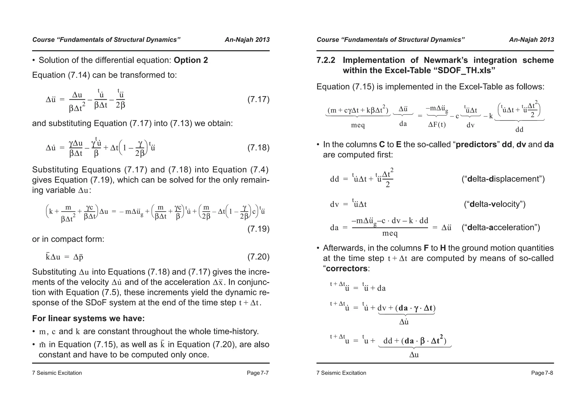
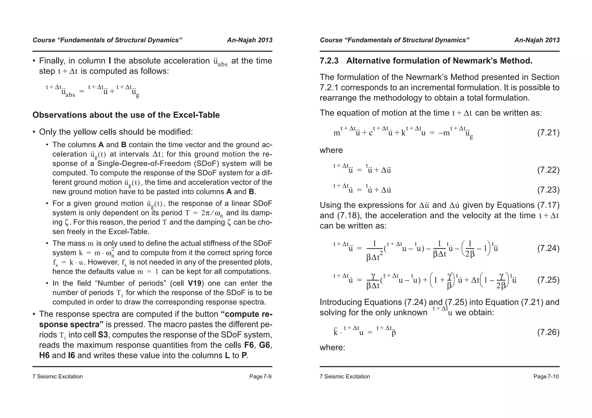
![Course “Fundamentals of Structural Dynamics” An-Najah 2013
7 Seismic Excitation Page7-11
(7.27)
(7.28)
(7.29)
(7.30)
(7.31)
This formulation corresponds to the implementation of New-
mark’s method presented in [Cho11].
k k a1+=
p
t Δt+
m u··t Δt+
g– a1 u
t
a2 u·t
a3 u··t
+ + +=
a1
m
βΔt
2
-----------
γc
βΔt
---------+=
a2
m
βΔt
---------
γ
β
--- 1–
© ¹
§ · c+=
a3
1
2β
------ 1–
© ¹
§ · m Δt
γ
2β
------ 1–
© ¹
§ · c+=
Course “Fundamentals of Structural Dynamics” An-Najah 2013
7 Seismic Excitation Page7-12
7.3 Time-history analysis of nonlinear SDoF systems
• Strength of the nonlinear SDoF system
(7.32)
• = force reduction factor
• = maximum spring force that a linear SDoF system of the
same period and damping would experience if submitted to
the same ground motion
• Maximum deformation of the nonlinear SDoF system
, hence (7.33)
• = yield displacement
• = displacement ductility
,fy
fel
Ry
------= μΔ
um
uy
------=
fy
fy
fel
Ry
------
kel uel⋅
Ry
------------------= =
Ry
fel fs
T ζ
u··
g
um
um μΔ uy⋅= μΔ um uy⁄=
uy
μΔ](https://image.slidesharecdn.com/fundamentalsofstructuraldynamics-200730194708/75/Fundamentals-of-structural-dynamics-69-2048.jpg)
![Course “Fundamentals of Structural Dynamics” An-Najah 2013
7 Seismic Excitation Page7-13
7.3.1 Equation of motion of nonlinear SDoF systems
In the equation of motion for a base point excitation through an
acceleration time-history
(7.34)
of a nonlinear SDoF system, the spring force is no longer
constant and varies in function of time and location.
Most structural components are characterised by a continuously
curved force-deformation relationship like the one shown by
means of a thin line on the right of the figure on page 7-12, which
however is often approximated by a bilinear curve (thick line in
the same figure).
When the loading of the nonlinear SDoF system is cyclic, then
is no longer an unambiguous function of the location and also
for this reason Equation (7.34) shall be solved incrementally.
For this reason must be described in such a way, that
starting from a known spring force at the time , the still
unknown spring force at the time can eas-
ily be computed.
This description of the cyclic force-deformation relationship is
known as hysteretic rule. In the literature many different hyster-
etic rules for nonlinear SDoF systems are available (See e.g.
[Saa91]).
In the following section a few hysteretic rules are presented and
discussed.
u··
g t( )
mu·· cu· fs u t( , )+ + mu··
g–=
fs u t( , )
fs
u
fs u t( , )
fs u t( , ) t
fs x Δu+ t Δt+( , ) t Δt+
Course “Fundamentals of Structural Dynamics” An-Najah 2013
7 Seismic Excitation Page7-14
7.3.2 Hysteretic rules
The next figure shows typical hysteretic rules (or models) for
nonlinear SDoF systems.](https://image.slidesharecdn.com/fundamentalsofstructuraldynamics-200730194708/75/Fundamentals-of-structural-dynamics-70-2048.jpg)
![Course “Fundamentals of Structural Dynamics” An-Najah 2013
7 Seismic Excitation Page7-15
In the following the often used Takeda hysteretic model is dis-
cussed in some detail.
The Takeda model was first described in [TSN70] and later mod-
ified by various authors. The assumed force-deformation rela-
tionship shown in the following figure was derived from the mo-
ment-curvature relationship described in [AP88].
The initial loading follows the bilinear force-deformation relation-
ship for monotonic loading mentioned in the previous section.
The exact definition of this so-called skeleton curve depends on
the structural element at hand. For example, in the case of Re-
inforced Concrete (RC) structural walls the elastic stiffness
corresponds to 20 to 30% of the uncracked stiffness, while the
plastic stiffness is approximated assuming an hard-
ening factor .
Large amplitude cycles
fs
u
ξp
+
β ξ⋅ p
+
β ξ⋅ p
+
uy
fy
β > 0 β < 0
ku
+
ku
-
kel
kpl=ro·kel
urev
urev
A+ B+ A+
fs
u
Small amplitude cycles
β > 0
ku
+
ku
-
kpl=ro·kel
urevurec
-
urec
+
β < 0
A+ B+
C+
B-
C-
β ξ⋅ p
+
β ξ⋅ p
-
β ξ⋅ p
-
x- x-
X-X-
kel
kpl ro k⋅= el
ro 0.01…0.05=
Course “Fundamentals of Structural Dynamics” An-Najah 2013
7 Seismic Excitation Page7-16
Unloading occurs along a straight line with stiffness . This un-
loading stiffness is computed by means of Equation (7.35) as a
function of the elastic stiffness and taking into softening ef-
fects in proportion of the previously reached maximum displace-
ment ductility . The parameter controls the unloading stiff-
ness reduction and varies from structural element to structural
element.
, (7.35)
Reloading follows a straight line which is defined by the force re-
versal point and the point A. The location of point A is de-
termined according to the figure on the previous page as a func-
tion of the last reversal point B, the plastic strain and the dam-
age influence parameter . The parameter allows taking into
account softening effects occurring during the reloading phase.
Again, in the case of RC walls meaningful parameters and
lay in the following ranges: and .
These rules, which are valid for cycles with large amplitude, are
typically based on observations of physical phenomena made
during experiments.
On the other hand, rules for small amplitude cycles are based on
engineering considerations rather than on exact observations.
They are designed to provide reasonable hysteresis lops during
an earthquake time-history, thus avoiding clearly incorrect be-
haviours like e.g. negative stiffnesses.
The rules for small amplitude cycles are shown on the right of the
figure on the previous page.
ku
kel
μΔ α
ku
+ kel max μΔ
+{ }( )
α–
⋅= ku
- kel max μΔ
-{ }( )
α–
⋅=
urev 0( , )
ξp
β β
α β
α 0.2…0.6= β 0.0… 0.3–=](https://image.slidesharecdn.com/fundamentalsofstructuraldynamics-200730194708/75/Fundamentals-of-structural-dynamics-71-2048.jpg)
![Course “Fundamentals of Structural Dynamics” An-Najah 2013
7 Seismic Excitation Page7-17
If a reloading phase starts from a force reversal point lay-
ing between the two extreme force reversal point and
, then reloading does no longer occurs towards point A,
but towards a newly calculated point X, which lies between
points A and B. The position of point X is calculated using the
auxiliary variables and defined in Equation (7.36).
, (7.36)
When a load reversal occurs before point X is reached, a new
point C is defined as a temporary maximum and minimum. The
reloading in the subsequent cycles, which are smaller than the
temporary maximum and minimum is then always in the direc-
tion of point C.
These rules for cycles with a small amplitude are a simplification
of those described in [AP88], however they lead to very satisfac-
tory results and can be programmed very easily and efficiently.
urev 0( , )
urec
+
0( , )
urec
-
0( , )
x
+
x
-
x
+ urev urec
+
–
urec
-
urec
+
–
-------------------------
© ¹
¨ ¸
§ ·
βξp
+
⋅= x
- urev urec
-
–
urec
+
urec
-
–
-------------------------
© ¹
¨ ¸
§ ·
βξp
-
⋅=
Course “Fundamentals of Structural Dynamics” An-Najah 2013
7 Seismic Excitation Page7-18
7.3.3 Newmark’s method for inelastic systems
The Newmark’s numerical method discussed in Sections 7.2.1
to 7.2.3 can be easily modified for application to nonlinear sys-
tems. The following modifications are required:
• The mass and the damping are typically constant through-
out the whole time-history.
• The stiffness changes during the time-history, hence , re-
spectively , are no longer constant.
• If the stiffness changes within the time step iterations are need-
ed (e.g. Newton-Raphson).
• For nonlinear systems the second solution strategy presented
in Section 7.2.1 (Option 2) has the advantage that the factors
and
on the RHS of Equation (7.19) are constant throughout the
whole time-history and do not need to be recomputed at every
time step.
Remark
For the actual implementation of the nonlinear version of New-
mark’s time stepping method, it is suggested to use the formula-
tion presented in Section 7.4.4 in conjunction with the Newton-
Raphson algorithm described in Section 7.4.3.
m c
k m˜
k
a
m
βΔt
---------
γc
β
-----+
© ¹
§ ·= b
m
2β
------ Δt 1
γ
2β
------–
© ¹
§ · c–=](https://image.slidesharecdn.com/fundamentalsofstructuraldynamics-200730194708/75/Fundamentals-of-structural-dynamics-72-2048.jpg)
![Course “Fundamentals of Structural Dynamics” An-Najah 2013
7 Seismic Excitation Page7-19
7.3.4 Example 1: One-storey, one-bay frame
, , , (7.37)
• Parameters
Columns k [kN/m] T [s] fy [MPa] Vy [kN] Vy/Vel [-] Δy [cm]
HEA 100 141 3.75 595 39.5 1.00 28.1
HEA 100 141 3.75 298 19.8 0.50 14.0
HEA 100 141 3.75 149 9.9 0.25 7.0
HEA 100 141 3.75 99 6.6 0.167 4.7
HEA 220 2181 0.95 543 246.7 1.00 11.3
HEA 220 2181 0.95 272 123.4 0.50 5.7
HEA 220 2181 0.95 136 61.7 0.25 2.8
HEA 220 2181 0.95 91 41.1 0.167 1.9
IPE 550 27055 0.27 185 411.4 1.00 1.52
IPE 550 27055 0.27 93 205.7 0.50 0.76
IPE 550 27055 0.27 43 102.9 0.25 0.38
IPE 550 27055 0.27 31 68.6 0.167 0.25
k 2
12EIs
H
3
--------------⋅= T 2π
m
k
----= Vy 2
My
H 2⁄
-----------⋅= Δy
Vy
k
------=
Course “Fundamentals of Structural Dynamics” An-Najah 2013
7 Seismic Excitation Page7-20
• Frames with , subjected to “El Centro”T 3.75s= ζ 5%=
0 10 20 30
−20
0
20
Displacement[cm]
−20 0 20
−40
−20
0
20
40
Shearforce[kN]
Vel=39.5kN
0 10 20 30
−20
0
20
Displacement[cm]
−20 0 20
−40
−20
0
20
40
Shearforce[kN]
Vy=19.8kN
0 10 20 30
−20
0
20
Displacement[cm]
−20 0 20
−40
−20
0
20
40
Shearforce[kN]
Vy=9.9kN
0 10 20 30
Time [s]
−20
0
20
Displacement[cm]
−20 0 20
Displacement [cm]
−40
−20
0
20
40
Shearforce[kN]
Vy=6.6kN
Δ=28.1cm
Δ=25.9cm
Δ=21.6cm
Δ=21.2cm](https://image.slidesharecdn.com/fundamentalsofstructuraldynamics-200730194708/75/Fundamentals-of-structural-dynamics-73-2048.jpg)
![Course “Fundamentals of Structural Dynamics” An-Najah 2013
7 Seismic Excitation Page7-21
• Frames with , subjected to “El Centro”T 0.95s= ζ 5%=
0 10 20 30
−10
0
10
Displacement[cm]
−10 0 10
−200
0
200
Shearforce[kN]
Vel=246.7kN
0 10 20 30
−10
0
10
Displacement[cm]
−10 0 10
−200
0
200
Shearforce[kN]
Vy=123.4kN
0 10 20 30
−10
0
10
Displacement[cm]
−10 0 10
−200
0
200
Shearforce[kN]
Vy=61.7kN
0 10 20 30
Time [s]
−10
0
10
Displacement[cm]
−10 0 10
Displacement [cm]
−200
0
200
Shearforce[kN]
Vy=41.1kN
Δ=11.3cm
Δ=7.7cm
Δ=9.4cm
Δ=10.4cm
Course “Fundamentals of Structural Dynamics” An-Najah 2013
7 Seismic Excitation Page7-22
• Frames with , subjected to “El Centro”T 0.27s= ζ 5%=
0 10 20 30
−2
−1
0
1
2
Displacement[cm]
−2 −1 0 1 2
−400
−200
0
200
400
Shearforce[kN]
Vel=411.4kN
0 10 20 30
−2
−1
0
1
2
Displacement[cm]
−2 −1 0 1 2
−400
−200
0
200
400
Shearforce[kN]
Vy=205.7kN
0 10 20 30
−2
−1
0
1
2
Displacement[cm]
−2 −1 0 1 2
−400
−200
0
200
400
Shearforce[kN]
Vy=102.9kN
0 10 20 30
Time [s]
−2
−1
0
1
2
Displacement[cm]
−2 −1 0 1 2
Displacement [cm]
−400
−200
0
200
400
Shearforce[kN]
Vy=68.6kN
Δ=1.5cm
Δ=1.2cm
Δ=1.5cm
Δ=2.2cm](https://image.slidesharecdn.com/fundamentalsofstructuraldynamics-200730194708/75/Fundamentals-of-structural-dynamics-74-2048.jpg)
![Course “Fundamentals of Structural Dynamics” An-Najah 2013
7 Seismic Excitation Page7-23
7.3.5 Example 2: A 3-storey RC wall
As a second example, the behaviour of the RC wall WDH4 pre-
sented in Section 7.6.3 is simulated. Wall WDH4 is actually a 3-
DoF system and its behaviour is simulated by means of an equiv-
alent SDoF system. For this reason the relative displacement of
the SDoF system shall be multiplied by the participation factor
to obtain an estimation of top displacement of WDH4.
To simulate the behaviour of WDH4 a nonlinear SDoF system
with Takeda hysteretic model is used. The parameter used to
characterise the SDoF system are:
, , , ,
, (7.38)
where is the damping rate, is the natural frequency of the
SDoF system for elastic deformations (i.e. with ), and
is the force reduction factor. The parameters given in (7.38) were
subsequently adjusted to obtain the best possible match be-
tween the simulation and the experiment. In a first phase, a cal-
culation using a linear SDoF system is performed. The latter has
the same damping rate and natural frequency as the Takeda
SDoF system and allows an estimation of the maximum elastic
spring force and of the maximum elastic deformation . The
yield force and the yield displacement of the Takeda SDoF
system are then estimated using the force reduction factor as
follows:
(7.39)
Γ˜ 1.291=
ζ 5%= fn 1.2Hz= Ry 2.5= ro 0.03=
α 0.2= β 0.15–=
ζ fn
k kel= Ry
fel uel
fy uy
Ry
Ry
fel
fy
-----
uel
uy
------= =
Course “Fundamentals of Structural Dynamics” An-Najah 2013
7 Seismic Excitation Page7-24
Time-history of the top displacement
The time-history of the top displacement (see below) shows that:
(i) plastic phenomena affect the behaviour of the wall WDH4 sig-
nificantly, and that (ii) the Takeda-SDoF System is able can de-
scribe the global behaviour of the wall WDH4 quite accurately.
-80
-60
-40
-20
0
20
40
60
80
WDH4: Experiment
Linear SDoF System
fn=1.2Hz, ζ=5%
fn=1.2Hz, ζ=5%, Ry=2.5,
ro=0.03, α=0.2, β=-0.15
Relativedisplacement[mm]
210 54321 54321 54321 543 7 10986 131211 161514 1817
Time [s]
-80
-60
-40
-20
0
20
40
60
80
Relativedisplacement[mm]
210 54321 54321 54321 543 7 10986 131211 161514 1817
Time [s]
WDH4: Experiment
Takeda SDoF System](https://image.slidesharecdn.com/fundamentalsofstructuraldynamics-200730194708/75/Fundamentals-of-structural-dynamics-75-2048.jpg)
![Course “Fundamentals of Structural Dynamics” An-Najah 2013
7 Seismic Excitation Page7-25
Hysteretic behaviour of the nonlinear SDoF System
Force-deformation relationship of the Takeda-SDoF System
subjected to the same ground motion as Wall WDH4. In both di-
agrams the same curve is plotted: On the left in absolute units
and on the right in normalised units.
-80
-60
-40
-20
0
20
40
60
80
-1.0
-0.5
0.0
0.5
1.0
Springforcef[kN]s
Relative displacement x [mm]
-80 -60 -40 -20 0 20 40
Normalisedspringforcef/f[kN]sy
Displacement dutility =u/u [mm]mD y
-2.5 -2.0 -1.5 -1.0 0.0 0.5 1.0-0.5 1.5
Course “Fundamentals of Structural Dynamics” An-Najah 2013
7 Seismic Excitation Page7-26
7.4 Solution algorithms for nonlinear analysis
problems
In this section the more general case of system with multiple de-
grees of freedom is discussed. SDoF system can be seen as a
special case thereof.
7.4.1 General equilibrium condition
The general equilibrium condition for elastic and inelastic static
and dynamic systems is:
(7.40)
In this equation is the time-dependent vector of the internal
forces of all DoFs of the structure and the time-dependent
vector of the external forces.
The vector depends on the problem analysed and is known.
7.4.2 Nonlinear static analysis
For linear-elastic systems the internal forces can be computed
by means of Equation (7.41):
(7.41)
where is the vector of the displacements of the DoF and is
the stiffness matrix of the structure. Equation (7.40) can there-
fore be rewritten as
(7.42)
F t( ) R t( )=
F t( )
R t( )
R t( )
F KU=
U K
KU R=](https://image.slidesharecdn.com/fundamentalsofstructuraldynamics-200730194708/75/Fundamentals-of-structural-dynamics-76-2048.jpg)
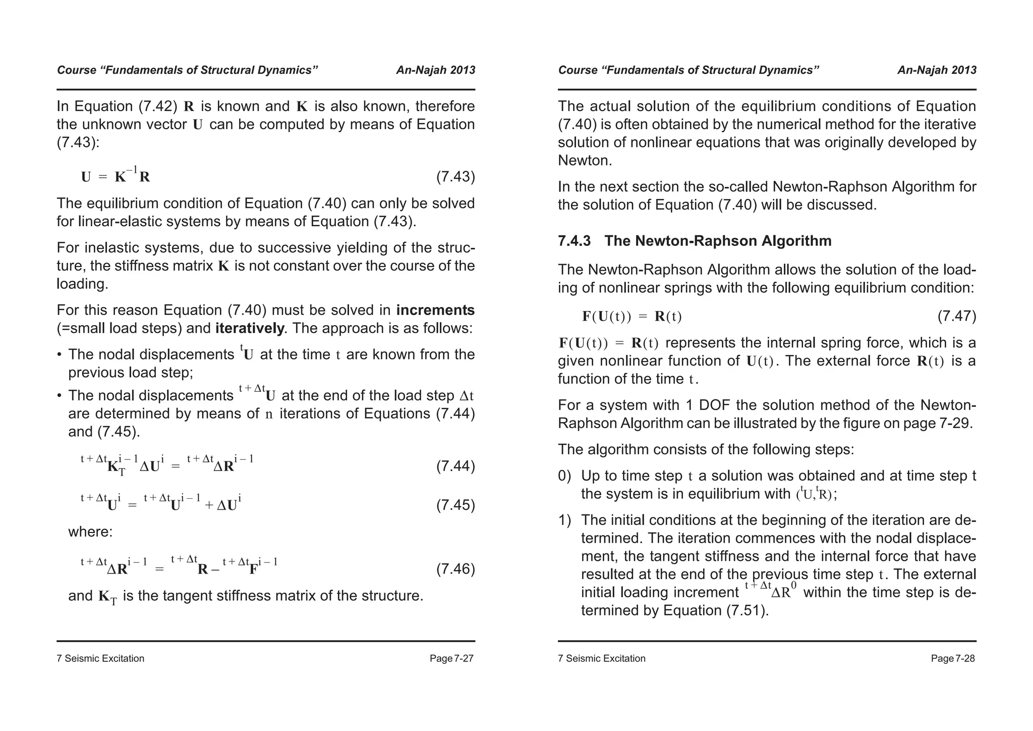
![Course “Fundamentals of Structural Dynamics” An-Najah 2013
7 Seismic Excitation Page7-29
Newton-Raphsonalgorithmtosolvesystemsofnonlinearequations(accordingto[AEM86])
U
R
tR
t+ΔtR
t+ΔtΔR0
tR=t+ΔtF0
tU=t+ΔtU0
t+ΔtKT
0
t+ΔtΔU1
t+ΔtKT
1
t+ΔtΔU2
t+ΔtKT
2
t+ΔtΔU3
t+ΔtU=t+ΔtUn
t+ΔtFn~t+ΔtF=t+ΔtR
t+ΔtU1
t+ΔtF1
t+ΔtΔR1
t+ΔtU2
t+ΔtF2
t+ΔtΔR2
Course “Fundamentals of Structural Dynamics” An-Najah 2013
7 Seismic Excitation Page7-30
ModifiedNewton-Raphsonalgorithmtosolvesystemsofnonlinearequations(accordingto[AEM86])
U
R
tR
t+ΔtR
t+ΔtΔR0
tR=t+ΔtF0
tU=t+ΔtU0
t+ΔtKT
0
t+ΔtΔU1t+ΔtΔU2
t+ΔtKT
0
t+ΔtU1
t+ΔtF1
t+ΔtΔR1
t+ΔtΔU3
t+ΔtKT
0
t+ΔtU=t+ΔtUn
t+ΔtFn~t+ΔtF=t+ΔtR
t+ΔtU2
t+ΔtF2
t+ΔtΔR2](https://image.slidesharecdn.com/fundamentalsofstructuraldynamics-200730194708/75/Fundamentals-of-structural-dynamics-78-2048.jpg)
![Course “Fundamentals of Structural Dynamics” An-Najah 2013
7 Seismic Excitation Page7-31
Displacement: (7.48)
Tangent stiffness: (7.49)
Internal force: (7.50)
External force: (7.51)
2) Computation of the ith
-displacement increment by
means of Equation (7.52) (i starts from 1).
For systems with more DoFs, is a matrix (tangent
stiffness matrix) and Equation (7.52) is best solved by means
of a -decomposition of the matrix .
(7.52)
3) Computation of the displacement at the end of the ith-
iteration
(7.53)
4) Computation of the internal force and the new external
force (residual force)
(7.54)
5) If and/or are so small that they can be neglected:
Continue with Step 7;
6) Determine the new tangent stiffness and repeat from
Step 2;
7) If the analysis time has not yet ended, start a new time step
and start again the procedure at Step 1.
U
t Δt+ 0
U
t
=
K
t Δt+ 0
T K
t
T=
F
t Δt+ 0
F
t
=
ΔR
t Δt+ 0
R F
t Δt+ 0
–
t Δt+
=
ΔU
i
K
t Δt+ i 1–
T
LDL
T
K
t Δt+ i 1–
T
K
t Δt+ i 1–
T ΔU
i
ΔR
t Δt+ i 1–
=
U
t Δt+ i
U
t Δt+ i
U
t Δt+ i 1–
ΔU
i
+=
F
t Δt+ i
R
t Δt+ i
ΔR
t Δt+ i
R F
t Δt+ i
–
t Δt+
=
ΔU
i
ΔR
t Δt+ i
K
t Δt+ i
T
Course “Fundamentals of Structural Dynamics” An-Najah 2013
7 Seismic Excitation Page7-32
Comments on the Newton-Raphson Algorithm
• The Newton-Raphson Algorithm for systems with several or
many DoFs follows exactly the same procedure as the algo-
rithm for SDoF systems. Only difference: Scalar values are re-
placed by the corresponding vectorial quantities.
• Apart from the Newton-Raphson Approach (“Full Newton-
Raphson iteration”) the “Modified Newton-Raphson iteration”
is often applied. This algorithm is illustrated on page 7-30.
• Unlike in the Newton-Raphson Algorithm, in the Modified Newton-
Raphson Algorithm the tangent stiffness matrix is updated only
at the beginning of the time step and is kept constant over all the
iterations within this time step.
• To reach the target displacement more iterations are re-
quired for the Modified Newton-Raphson Algorithm than for the
Full Newton-Raphson Algorithm. However, these can be comput-
ed more quickly since assembling the tangent stiffness matrix
(Step 6) and in particular its -decomposition (Step 2) are
only required at the beginning of a time step and not at each itera-
tion within the time step. This is particularly advantageous for sys-
tems with many DoFs.
• In most FE-analysis programs both Newton-Raphson Algo-
rithms as well as other algorithms are typically combined in a
general solver in order to obtain a successful convergence of
the iteration process for many structural analysis problems.
• Other algorithms for the solution of the equilibrium conditions
can be found in Chapters 8 (static analysis) and 9 (dynamic
analysis) of [Bat96].
KT
U
t Δt+
KT
LDL
T](https://image.slidesharecdn.com/fundamentalsofstructuraldynamics-200730194708/75/Fundamentals-of-structural-dynamics-79-2048.jpg)
![Course “Fundamentals of Structural Dynamics” An-Najah 2013
7 Seismic Excitation Page7-33
Convergence criteria
• A in-depth discussion of the convergence criteria can be found
in [Bat96] and [AEM86]. This section provides only a short
overview.
• In Step 5) criteria are required in order to decide whether con-
vergence of the iteration was obtained. Possible convergence
criteria can be based on displacements, force or energy con-
siderations.
• Since within the time step the unknown target displacement
needs to be determined, it makes sense to prescribe that
the target displacement is reached within a certain tolerance
interval. For this reason a possible displacement criterion for
the convergence is:
(7.55)
where is the displacement convergence tolerance.
• The vector is actually unknown and must therefore be ap-
proximated. Typically is used in conjunction with a suffi-
ciently small value of .
• It is important to note that in some cases – although the criteria de-
scribed by Equation (7.55) is satisfied – the wanted target dis-
placement has not been reached.
• This is the case when the computed displacements vary only
slightly during one iteration but these small increments are repeat-
ed over many iterations.
• Such a situation can result when the modified Newton-Raphson
Algorithm is used (see page 7-30).
U
t Δt+
ΔU
i
U
t Δt+
------------------- εD≤
εD
U
t Δt+
U
t Δt+ i
εD
U
t Δt+
Course “Fundamentals of Structural Dynamics” An-Najah 2013
7 Seismic Excitation Page7-34
• For this reason the displacement criterion is typically used in con-
junction with other convergence criteria.
• A force criterion, which checks the residual forces, is given in
Equation (7.56).
(7.56)
is the force convergence tolerance, which checks the mag-
nitude of the residual force after the ith-iteration against the first
load increment of the time step.
• As for the displacement criterion, this force criterion should not be
applied on its own because in some cases the target displacement
may not have been reached. This may happen for systems
with small post-yield stiffness.
• The energy criterion in Equation (7.57) has the advantage
that it checks the convergence of the displacements and the
forces simultaneously.
(7.57)
is the energy convergence tolerance, which checks the
work of the residual forces of the ith
-iteration against the work
of the residual forces of the first load increment of the time
step.
Choosing the tolerances , or too large, can yield wrong
results, which can lead to the divergence of the solution in the
following load steps.
R F
t Δt+ i
–
t Δt+
R F
t
–
t Δt+
---------------------------------------- εF≤
εF
U
t Δt+
ΔU
i
( )
T
R F
t Δt+ i 1–
–
t Δt+
( )
ΔU
1
( )
T
R F
t
–
t Δt+
( )
----------------------------------------------------------------- εE≤
εE
εD εF εE](https://image.slidesharecdn.com/fundamentalsofstructuraldynamics-200730194708/75/Fundamentals-of-structural-dynamics-80-2048.jpg)
![Course “Fundamentals of Structural Dynamics” An-Najah 2013
7 Seismic Excitation Page7-35
Choosing the tolerances , or too small, results in an un-
necessary increase of the required iteration steps. The in-
creased accuracy is typically not useful.
For numerical reasons it can also happen that too small con-
vergence tolerances do not allow to reach convergence at all.
For strongly inelastic systems it is recommended to check
the sensitivity of the results to the chosen convergence
criteria and the chosen tolerances.
7.4.4 Nonlinear dynamic analyses
Similar to Equation (7.44) the equilibrium condition for nonlinear
dynamic analyses is:
(7.58)
(7.59)
For base excitation by means of ground accelerations the vector
of the external forces is computed according to Equation (7.60).
(7.60)
where is the mass matrix of the structure, the norm vector
with entries of unity for all DoFs in the direction of the excitation
and the ground acceleration at the time .
For this type of excitation the differential equation of motion
(7.58) has to be integrated numerically and – due to the inelas-
tic behaviour of the system – the equation must be solved itera-
tively and incrementally.
εD εF εE
M U··t Δt+ i
C U·t Δt+ i
F
t Δt+ i 1–
K
t Δt+ i 1–
T ΔU
i
+( )+ + R
t Δt+
=
U
t Δt+ i
U
t Δt+ i 1–
ΔU
i
+=
R
t Δt+
M– 1 a
t Δt+
g=
M 1
a
t Δt+
g t Δt+
Course “Fundamentals of Structural Dynamics” An-Najah 2013
7 Seismic Excitation Page7-36
The numerical time integration of Equation (7.58) is often per-
formed by means of the Newmark’s Algorithms ([New 59]). Ac-
cording to these algorithms the displacement vector at the time
is estimated as follows:
(7.61)
(7.62)
From Equation (7.61):
(7.63)
Substituting Equation (7.63) into (7.62):
(7.64)
The expressions for the displacement, the velocity and the acceler-
ation at the time from Equations (7.59), (7.64) and (7.63) can
be substituted into the differential equation of motion (7.58) which
can then be solved for the only remaining unknown :
(7.65)
t Δt+
U
t Δt+
U
t
U·t
tΔ 1 2β–( ) U··t
2β U··t tΔ+
+[ ]
t
2
Δ
2
-------+ +=
U·t Δt+
U·t
1 γ–( ) U··t
γ U··t tΔ+
+[ ] tΔ+=
U··t tΔ+ 1
β t
2
Δ
----------- U
t tΔ+
U
t
–( )
1
β tΔ
-------- U·t
–
1 2– β
2β
-------------
© ¹
§ · U··t
–=
U·t tΔ+ γ
β tΔ
-------- U
t tΔ+
U
t
–( ) 1
γ
β
---–
© ¹
§ · U·t
1
γ
2β
------–
© ¹
§ · U··t
tΔ+ +=
t Δt+
ΔU
i
K
t Δt+ i 1–
T
1
βΔt
2
-----------M
γ
βΔt
---------C+ +
© ¹
§ · ΔU
i
R
t Δt+
F
t Δt+ i 1–
–
M
1
βΔt
2
----------- U
t Δt+ i 1–
U
t
–( )
1
βΔt
--------- U·t
–
1
2β
------ 1–
© ¹
§ · U··t
–
–
C
γ
βΔt
--------- U
t Δt+ i 1–
U
t
–( ) 1
γ
β
---–
© ¹
§ · U·t
1
γ
2β
------–
© ¹
§ · U··t
tΔ+ +
–
=](https://image.slidesharecdn.com/fundamentalsofstructuraldynamics-200730194708/75/Fundamentals-of-structural-dynamics-81-2048.jpg)
![Course “Fundamentals of Structural Dynamics” An-Najah 2013
7 Seismic Excitation Page7-37
or in a more compact format:
(7.66)
Equation (7.66) corresponds exactly to Equation (7.44) and is
also solved iteratively by the Newton-Raphson Algorithm.
When dynamic analyses are carried out, typical convergence
criteria also consider the inertia forces and, if present, damping
forces. Possible, often used convergence criteria are:
(7.67)
(7.68)
with
(7.69)
As alternative, depending at which point during the iteration proc-
ess convergence is checked, both criteria can be rewritten as:
(7.70)
(7.71)
As for static analyses, different convergence criteria exist also
for dynamic analyses and a discussion of these can also be
found in [Bat96].
K
˜
t tΔ+ i 1–
T U
i
Δ RΔ
˜
t tΔ+ i 1–
=
R
t Δt+
F
t Δt+ i 1–
– M U··t Δt+ i 1–
– C U·t Δt+ i 1–
–
RNORM
------------------------------------------------------------------------------------------------------------------- εF≤
ΔU
i
( )
T
R
t Δt+
F
t Δt+ i 1–
– M U··t Δt+ i 1–
– C U·t Δt+ i 1–
–( )
ΔU
1
( )
T
R
t Δt+
F
t
M U··t
– C U·t
––( )
------------------------------------------------------------------------------------------------------------------------------------- εE≤
RNORM mij¦ g⋅=
R
t Δt+
F
t Δt+ i
– M U··t Δt+ i
– C U·t Δt+ i
–
RNORM
----------------------------------------------------------------------------------------------- εF≤
ΔU
i
( )
T
R
t Δt+
F
t Δt+ i
– M U··t Δt+ i
– C U·t Δt+ i
–( )
ΔU
1
( )
T
R
t Δt+
F
t
M U··t
– C U·t
––( )
----------------------------------------------------------------------------------------------------------------- εE≤
Course “Fundamentals of Structural Dynamics” An-Najah 2013
7 Seismic Excitation Page7-38
7.4.5 Comments on the solution algorithms for nonlinear
analysis problems
• Contrary to the analysis of elastic systems, the analysis of in-
elastic systems is often interrupted before the targeted load or
deformation state is reached.
• This situation arises if in one of the time steps convergence cannot
be reached.
• Typical causes for the failing convergence
• The convergence tolerances are too small or too large;
• The chosen values for the parameters of the solution algorithm are
not appropriate;
• The solution algorithm is not suitable.
Typical example: If special measures are not taken, the algorithms
of the Newton family are not able to solve a system with a global
negative post-yield stiffness;
• Apart from the algorithms by Newmark, many other algorithms
have been developed for solving the differential equation of
motion (7.58) (e.g. “Houbolt Method”, “Wilson θ Method”, “α-
Method”). These methods are described in detail in [Bat96].
The “α-Method” allows to introduce numerical damping, which
can be useful. The “α-Method” is described in detail in
[HHT77].
• Choice of the time step for static analyses:
• For static analyses the time has no physical meaning. For this rea-
son the size of the time step can be chosen almost arbitrarily.
• As long as the algorithm converges and the variation of the exter-
nal loads is captured correctly, the size of the time step has only
a minor influence on the results.
Δt
t
Δt
Δt](https://image.slidesharecdn.com/fundamentalsofstructuraldynamics-200730194708/75/Fundamentals-of-structural-dynamics-82-2048.jpg)
![Course “Fundamentals of Structural Dynamics” An-Najah 2013
7 Seismic Excitation Page7-39
• However, when geometric nonlinearities are considered or when
the constitutive laws are a function of the strain history, care should
be taken also for static analyses when choosing the size of the
time step.
• The time step size influences the convergence of the algorithm:
For small the algorithm converges more quickly; however, more
steps are required.
• Time steps of a variable size can be advantageous. If the system
is elastic or almost elastic, large times steps can be chosen. If the
system is close to its capacity, small time steps should be chosen.
• Certain analysis programs (see for example [HKS03]) determine
the time step size within chosen limits as a function of the conver-
gence and the number of required iterations.
• Choice of the time step for dynamic analyses
• The objective of the dynamic analyses is the solution of the differ-
ential equation of motion (7.58) between the time and the time
. For this reason the choice of the time step plays always
an important role regarding the accuracy of the solution.
• The accuracy of the integration of the differential equation of mo-
tion (7.58) depends on the chosen time-integration algorithm and
on the ratio given by Equation (7.72), where are the natural pe-
riods of the system. To capture the motion components due to
higher modes the time step has therefore to be reduced.
(7.72)
• Certain time-integration algorithms can become instable if the time
step size is too large.
Δt
Δt
t
t Δt+ Δt
Tn
Δt
Δt
Tn
------
Δt
Course “Fundamentals of Structural Dynamics” An-Najah 2013
7 Seismic Excitation Page7-40
• An in-depth discussion on the accuracy of time-integration meth-
ods and on so-called “conditionally stable” integration methods
can be found in [Bat96].
• Example:
The time-integration method by Newmark with and
(linear variation of the acceleration over the length of the
time step, see Section 7.2.1) is only stable if the criterion given in
Equation (7.73) is met for all natural periods of the system. For
systems with many DoFs, higher modes can be especially prob-
lematic and a very short time step is generally required when this
time-integration method is used.
(7.73)
• For this reason the “unconditionally stable” time-integration algo-
rithm by Newmark with and is often used in
seismic engineering.
γ 1 2⁄=
β 1 6⁄=
Tn
Δt
Tn
------ 0.551≤
γ 1 2⁄= β 1 4⁄=](https://image.slidesharecdn.com/fundamentalsofstructuraldynamics-200730194708/75/Fundamentals-of-structural-dynamics-83-2048.jpg)
![Course “Fundamentals of Structural Dynamics” An-Najah 2013
7 Seismic Excitation Page7-41
7.4.6 Simplified iteration procedure for SDoF systems with
idealised rule-based force-deformation relationships
In the case that the hysteretic behaviour is described by a se-
quence of straight lines, a so called “idealized rule-based force-
deformation relationships” like the Takeda model presented in
Section 7.3.2, it is possible to avoid implementing a Newton-
Raphson Iteration strategy. In this case adjustments are needed
in the case of:
• Stiffness change during loading
• Velocity reversal
• Transition between unloading an reloading.
In first case a secant stiffness can be iteratively computed until
the target point lays on the backbone curve, while in the second
and third case it is often enough to reduce the size of the time
step to limit error. These strategies are shown in the following fig-
ure:
Course “Fundamentals of Structural Dynamics” An-Najah 2013
7 Seismic Excitation Page7-42
7.5 Elastic response spectra
7.5.1 Computation of response spectra
• Response spectra are used to represent the seismic demand
on structures due to a ground motion record and design spec-
tra are used for the seismic design of structures.
• Response spectra shall be computed for all periods and
damping rates likely to be found in structures.
• Unless specified otherwise, the response spectra presented in
the following belongs to the north-south component of the May
18, 1940 “El Centro” Earthquake (see [Cho11]).
• Additional ground motion records can be downloaded for free
from:
1) http://db.cosmos-eq.org/scripts/default.plx
2) http://peer.berkeley.edu/nga/](https://image.slidesharecdn.com/fundamentalsofstructuraldynamics-200730194708/75/Fundamentals-of-structural-dynamics-84-2048.jpg)
![Course “Fundamentals of Structural Dynamics” An-Najah 2013
7 Seismic Excitation Page7-43
• “El Centro”: Linear response spectra
0.01 0.10 1.00 10.00 100.0
0
10
20
30
40
Absoluteacceleration[m/s2
]
0.01 0.10 1.00 10.00 100.0
0
1
2
3
Relativevelocity[m/s]
0.01 0.10 1.00 10.00 100.0
Period [s]
0.1
0.2
0.3
0.4
0.5
0.6
Relativedisplacement[m]
ζ 0%=
ζ 2%=
ζ 5%=
ζ 10%=
ζ 20%=
ζ 0%=
ζ 2%=
ζ 5%=
ζ 10%=
ζ 20%=
ζ 0%=
ζ 2%=
ζ 5%=
ζ 10%=
ζ 20%=
Course “Fundamentals of Structural Dynamics” An-Najah 2013
7 Seismic Excitation Page7-44
• Limits of response spectra
u··
a 2ζωu· ω2u++ 0=
u 0 u··
a t( )Ÿ u·· t( ) u··
g t( )+ u··
g t( )= = =
u··
a 2ζωu· ω2u++ 0=
u·· t( ) u··– g t( ) u t( )Ÿ u– g t( )= =
0 10 20 30
−2.0
0.0
2.0
ag[m/s2
]
0 10 20 30
−0.2
0.0
0.2
0.4
vg[m/s]
0 10 20 30
Time [s]
−0.1
0.0
0.1
0.2
dg[m]
vg,max = 36.1cm/s
dg,max = 21.1cm
ag,max = 3.13 m/s2
Baseline
correction!](https://image.slidesharecdn.com/fundamentalsofstructuraldynamics-200730194708/75/Fundamentals-of-structural-dynamics-85-2048.jpg)
![Course “Fundamentals of Structural Dynamics” An-Najah 2013
7 Seismic Excitation Page7-45
7.5.2 Pseudo response quantities
• Pseudo-velocity
(7.74)
- has units of a velocity
- is related to the peak value of the strain energy
(7.75)
• Pseudo-acceleration
(7.76)
- has units of an acceleration
- is related to the peak value of the base shear
(7.77)
Spv
Spv ωSd=
Spv
Spv Es
Es
kSd
2
2
---------
k Spv ω⁄( )
2
2
---------------------------
mSpv
2
2
-------------= = =
Spa ω2Sd=
Spa
Spa V
V kSd k Spa ω2⁄( ) mSpa= = =
Course “Fundamentals of Structural Dynamics” An-Najah 2013
7 Seismic Excitation Page7-46
• True vs. Pseudo response quantities
• For are acceleration and pseudo-acceleration identical.
• For the pseudo-velocity tends to zero.
• Pseudo-velocity and pseudo-acceleration match well the true mo-
tion of a SDOF system with and
0.01 0.10 1.00 10.00 100.00
0
5
10
Absoluteacceleration[m/s2
]
0.01 0.10 1.00 10.00 100.00
Periode [s]
0.0
0.5
1.0
Relativevelocity[m/s]
Acceleration
Pseudo-acceleration
Velocity
Pseudo-velocity
ζ = 5%
ζ = 50%
ζ = 5%
ζ = 50%
ζ 0=
T ∞Ÿ
ζ 20%< T 1s<](https://image.slidesharecdn.com/fundamentalsofstructuraldynamics-200730194708/75/Fundamentals-of-structural-dynamics-86-2048.jpg)
![Course “Fundamentals of Structural Dynamics” An-Najah 2013
7 Seismic Excitation Page7-47
• Remarks on the Pseudo-acceleration
• For :
• For : At : however
Shift of the location of the maxima through damping
(7.78)
0 5 10 15
−1.0
0.0
1.0
.../...max[−]
0 5 10 15
Time [s]
−1.0
0.0
1.0
.../...max[−]
Pseudo-acceleration
Pseudo-velocity
-1 x Displacement
Pseudo-acceleration
Pseudo-velocity
-1 x Displacement
ζ=0
ζ>0
u··
a t( ) ω2u t( )– 2ζωu· t( )–=
Time-history of the pseudo-acceleration A(t)
ζ 0= u t( ) A t( )=
ζ 0> umax ua A= A Amax<
Course “Fundamentals of Structural Dynamics” An-Najah 2013
7 Seismic Excitation Page7-48
• Combined D-V-A spectra
Spv ωSd= Spv( )log ω( )log Sd( )log+=
Spv( )log f( )log 2π( )log Sd( )log+ +=
Spv( )log T( )log– 2π( )log Sd( )log+ +=
Spv
Spa
ω
--------= Spv( )log ω( )log– Spa( )log+=
Spv( )log f( )log– 2π( )log– Spa( )log+=
Spv( )log T( )log 2π( )log– Spa( )log+=
0.1 1.0 10.0
Period [s]
1
10
100
Pseudo−velocitySpv[cm/s]
D
isplacem
entS
d
[cm
]
0.1
1
10
100
Pseudo−acc.Spa
[cm
/s
2]
1
10
100
1000
10000
Spv = 71 cm/s
T = 1 s
S
pa=
447
cm
/s2
Sd
=
11.2
cm](https://image.slidesharecdn.com/fundamentalsofstructuraldynamics-200730194708/75/Fundamentals-of-structural-dynamics-87-2048.jpg)
![Course “Fundamentals of Structural Dynamics” An-Najah 2013
7 Seismic Excitation Page7-49
7.5.3 Properties of linear response spectra
• Response spectra typically show spectral regions where the re-
sponse is sensitive to different motion quantities, i.e. they show an
acceleration sensitive region (small periods), a displacement
sensitive region (large periods) and a velocity sensitive region
laying in between.
0.1 1.0 10.0
Period [s]
1
10
100
Pseudo−velocitySpv[cm/s]
D
isplacem
entS
d
[cm
]
0.1
1
10
100
Pseudo−acc.Spa
[cm
/s
2]
1
10
100
1000
10000a
g=
313
cm
/s2
vg = 36.1 cm/s
dg
=
21.1
cm
ζ 0%=
ζ 2%=
ζ 5%=
ζ 10%=
Course “Fundamentals of Structural Dynamics” An-Najah 2013
7 Seismic Excitation Page7-50
7.5.4 Newmark’s elastic design spectra ([Cho11])
T [s]
Spv/vg[-]
Spa
/ag
[-]
S
d/d
g[-]
T [s]
Spa/ag[-]](https://image.slidesharecdn.com/fundamentalsofstructuraldynamics-200730194708/75/Fundamentals-of-structural-dynamics-88-2048.jpg)
![Course “Fundamentals of Structural Dynamics” An-Najah 2013
7 Seismic Excitation Page7-51
• Newmark’s elastic design spectra
Median(50%) One sigma (84%)
Damping
2% 2.74 2.03 1.63 3.66 2.92 2.42
5% 2.12 1.65 1.39 2.71 2.30 2.01
10% 1.64 1.37 1.20 1.99 1.84 1.69
20% 1.17 1.08 1.01 1.26 1.37 1.38
0.1 1.0 10.0
Period [s]
1
10
100
Pseudo−velocitySpv[cm/s]
D
isplacem
entS
d
[cm
]
0.1
1
10
100
Pseudo−acc.Spa
[cm
/s
2]
1
10
100
1000
10000
a
g
vg
dg
α
aa
g αvvg
αd
dg
TA=1/33s TB=1/8s TE=10s
TF=33s
B
A
F
C
D
E
ζ = 5%
ζ αa αv αd αa αv αd
Course “Fundamentals of Structural Dynamics” An-Najah 2013
7 Seismic Excitation Page7-52
• Elastic design spectra according to SIA 261 (Art. 16.2.3)
• Ground class A: firm or soft rock with a maximum soil cover of 5m
• Ground class B: deposit of extensive cemented gravel and sand
with a thickness >30m.
• Ground class C: deposits of normally consolidated and unce-
mented gravel and sand with a thickness >30m.
• Ground class D: deposits of unconsolidated fine sand, silt and
clay with a thickness >30m.
• Ground class E: alluvial surface layer of GC C or D, with a thick-
ness of 5 to 30m above a layer of GC A or B.
• Ground class F: deposits of structurally-sensitive and organic
deposits with a thickness >10m.
0.01 0.10 1.00 10.00
Period [s]
0
1
2
3
4
5
6
Pseudo−accelerationSpa[m/s2
]
Zone 3b, ζ = 5%
Ground Class A
Ground Class B
Ground Class C
Ground Class D
Ground Class E](https://image.slidesharecdn.com/fundamentalsofstructuraldynamics-200730194708/75/Fundamentals-of-structural-dynamics-89-2048.jpg)
![Course “Fundamentals of Structural Dynamics” An-Najah 2013
7 Seismic Excitation Page7-53
• Displacement elastic design spectra according to SIA 261
• The displacement spectra are computed from the acceleration
spectra using equation (7.79)
(7.79)
• Displacement spectra are an important design tool (even within
force-based design procedures) because they allow a quick esti-
mate of the expected deformations, hence of the expected dam-
age.
0.01 0.10 1.00 10.00
Period [s]
0
5
10
15
20
25
DisplacementSd[cm]
Zone 3b, ζ = 5%
Ground Class A
Ground Class B
Ground Class C
Ground Class D
Ground Class E
Sd
Spa
ω
2
--------=
Course “Fundamentals of Structural Dynamics” An-Najah 2013
7 Seismic Excitation Page7-54
• Elastic design spectra according to SIA 261 (linear)
0.00 0.50 1.00 1.50 2.00 2.50 3.00
Period [s]
0
1
2
3
4
5
6
Pseudo−accelerationSpa[m/s2
]
Zone 3b, ζ = 5%
Ground Class A
Ground Class B
Ground Class C
Ground Class D
Ground Class E
0.00 0.50 1.00 1.50 2.00 2.50 3.00
Period [s]
0
5
10
15
20
25
DisplacementSd[cm]
Zone 3b, ζ = 5%
Ground Class A
Ground Class B
Ground Class C
Ground Class D
Ground Class E](https://image.slidesharecdn.com/fundamentalsofstructuraldynamics-200730194708/75/Fundamentals-of-structural-dynamics-90-2048.jpg)
![Course “Fundamentals of Structural Dynamics” An-Najah 2013
7 Seismic Excitation Page7-55
• Elastic design spectra: Newmark vs. SIA 261
• The SIA 261 spectra, like the spectra of the majority of the stand-
ards worldwide, were defined using the same principles as New-
mark’s spectra.
• However, different ground motion were used:
- SIA 261 takes into account different ground classes;
- Different seismic sources were considered;
- A larger number of ground motions was considered.
• Note: in SIA 261 the corner period is not defined.
0.01 0.10 1.00 10.00
Period [s]
0.0
0.5
1.0
1.5
2.0
2.5
3.0
3.5
Spa/Ag[−]
Elastic design spectrum according to
SIA 261, Ground Type A
Elastic design spectrum according to
SIA 261, Ground Type B
Newmark’s elastic design spectrum
ζ = 5%
A
B C
D
TA
Course “Fundamentals of Structural Dynamics” An-Najah 2013
7 Seismic Excitation Page7-56
7.5.5 Elastic design spectra in ADRS-format (e.g. [Faj99])
(Acceleration-Displacement-Response Spectra)
Periods T correspond to lines running through the origin of the
axes, because:
and after reorganizing:
0 5 10 15
Sd [cm]
0.0
0.1
0.2
0.3
0.4
0.5
Spa[g]
0 1 2 3 4 5
Period [s]
0
5
10
15
Sd[cm]
0 1 2 3 4 5
Period [s]
0.0
0.1
0.2
0.3
0.4
0.5
Spa[g]
Spa ω2Sd=
T = const.
Spa ω2Sd= T 2π Sd Spa⁄=](https://image.slidesharecdn.com/fundamentalsofstructuraldynamics-200730194708/75/Fundamentals-of-structural-dynamics-91-2048.jpg)
![Course “Fundamentals of Structural Dynamics” An-Najah 2013
7 Seismic Excitation Page7-57
• Elastic design spectra in ADRS-format
• Design spectra are defined based on averaged response spectra.
For this reason, the spectral values of single response spectra
may differ significantly from the design spectra.
• This is a crucial property of design spectra and should be
kept in mind during design!
0 5 10 15
Sd [cm]
0.0
0.1
0.2
0.3
0.4
0.5
Spa[g]
Elastic design spectrum of an
earthquake with equal ag,max
Elastic design spectrum according to
SIA 261, Ground Type B
ζ = 5%
T=0.87s: Underestimation
T=0.77s: Overestimation
Course “Fundamentals of Structural Dynamics” An-Najah 2013
7 Seismic Excitation Page7-58
7.6 Strength and Ductility
7.6.1 Illustrative example
Comparison of the time history analyses of an elastic and an in-
elastic single-degree-of-freedom system (SDOF system):
Where:
: Force reduction factor (7.80)
: Maximum restoring force that the elastic SDOF system
reaches over the course of the seismic excitation
(7.81)
: Yield force of the inelastic SDOF system (7.82)
:Displacement ductility (7.83)
: Maximum displacement that the inelastic SDOF system
reaches over the course of the seismic excitation
(7.84)
: Yield displacement of the inelastic SDOF system (7.85)
Telastic = Tinelastic
Ry
fel
fy
-----=
fel u··
g t( )
fy
μΔ
um
uy
------=
um u··
g t( )
uy](https://image.slidesharecdn.com/fundamentalsofstructuraldynamics-200730194708/75/Fundamentals-of-structural-dynamics-92-2048.jpg)
![Course “Fundamentals of Structural Dynamics” An-Najah 2013
7 Seismic Excitation Page7-59
• Results
0 5 10 15 20 25 30 35 40
Time [s]
-0.15
-0.10
-0.05
0.00
0.05
0.10
0.15
Displacement[m]
Elastic SDOF system
Inelastic SDOF system (Ry=2)
Inelastic SDOF system (Ry=6)
-0.15 -0.10 -0.05 0.00 0.05 0.10 0.15
Displacement [m]
-150
-100
-50
0
50
100
150
Force[kN]
Elastic SDOF system
Inelastic SDOF system (Ry=2)
Inelastic SDOF system (Ry=6)
Course “Fundamentals of Structural Dynamics” An-Najah 2013
7 Seismic Excitation Page7-60
• Comments
• Both inelastic SDOF systems show a stable seismic response.
Quantity Elastic SDOF Inela. SDOF Ry=2 Inela. SDOF Ry=6
T [s] 2.0 2.0 2.0
Fmax [kN] 134.70 67.35 22.45
Ry [-] – 2.0 6.0
uy [m] – 0.068 0.023
um [m] 0.136 0.147 0.126
μΔ [-] – 2.16 5.54](https://image.slidesharecdn.com/fundamentalsofstructuraldynamics-200730194708/75/Fundamentals-of-structural-dynamics-93-2048.jpg)
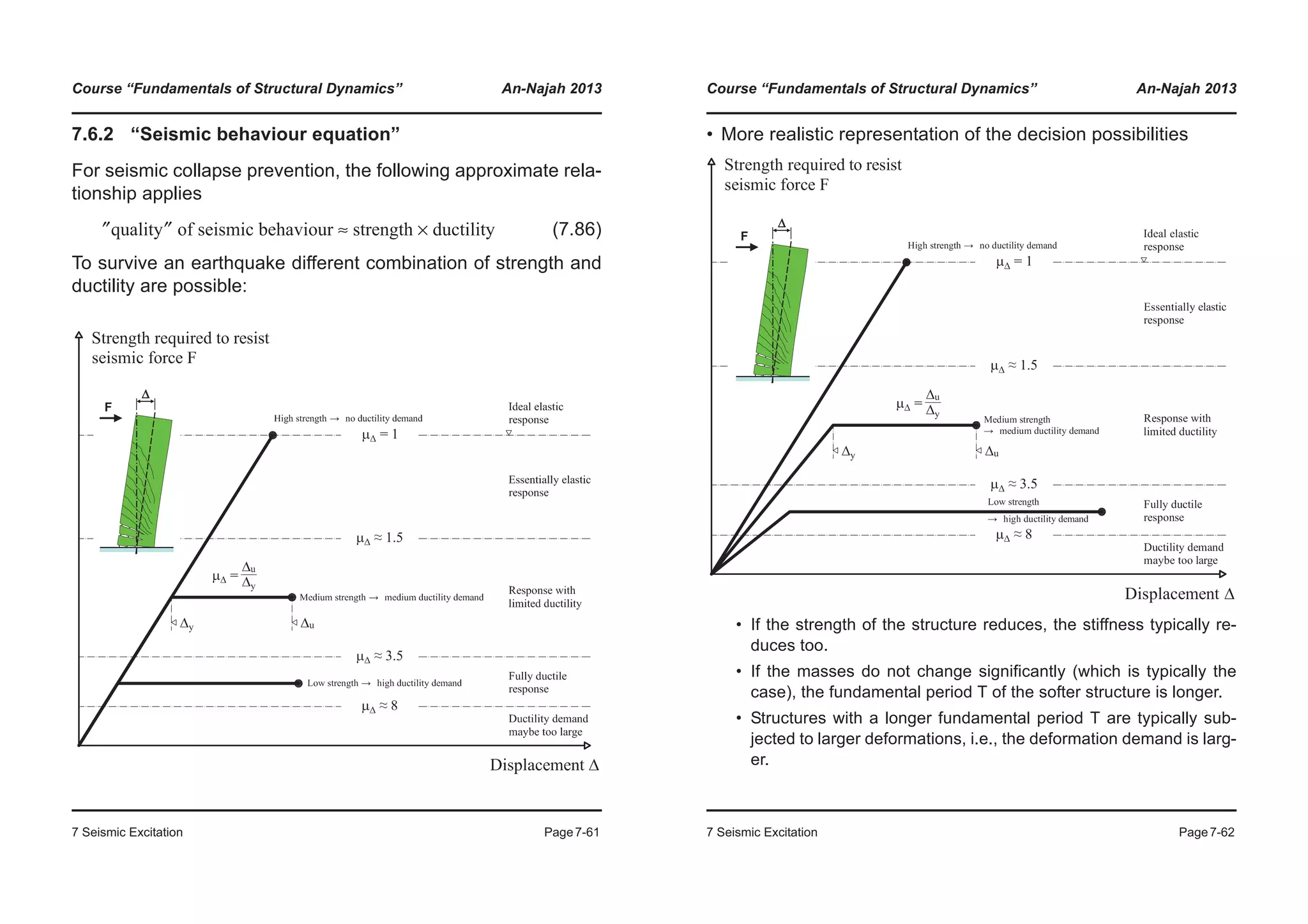
![Course “Fundamentals of Structural Dynamics” An-Najah 2013
7 Seismic Excitation Page7-63
7.6.3 Inelastic behaviour of a RC wall during an earthquake
• Moment-curvature-relation-
ship at the base of the plas-
tic hinge zone.
• Despite reaching and ex-
ceeding its elastic limit the
wall did not collapse.
• The plastic deformation ca-
pacity of structures can real-
ly be taken into account for
seismic design purposes.
−30 −20 −10 0 10 20 30
Curvature [1/km]
−100
−50
0
50
100
Moment[kNm]
Wall WDH4
Course “Fundamentals of Structural Dynamics” An-Najah 2013
7 Seismic Excitation Page7-64
7.6.4 Static-cyclic behaviour of a RC wall
Wall WSH6 [DWB99]](https://image.slidesharecdn.com/fundamentalsofstructuraldynamics-200730194708/75/Fundamentals-of-structural-dynamics-95-2048.jpg)
![Course “Fundamentals of Structural Dynamics” An-Najah 2013
7 Seismic Excitation Page7-65
• Hysteretic behaviour of the RC wall under static-cyclic loading
Plastic region of test unit WSH6 (left) and close-up of the left boundary region (right). Both pho-
tos were taken at displacement ductility 6.
−100 −80 −60 −40 −20 0 20 40 60 80 100
Top displacement [mm]
−500
−400
−300
−200
−100
0
100
200
300
400
500
Actuatorforce[kN]
−Fy
−0.75 Fy
0.75 Fy
Fy
μΔ=6 μΔ=5 μΔ=4 μΔ=3 μΔ=2 μΔ=1 μΔ=1 μΔ=2 μΔ=3 μΔ=4 μΔ=5 μΔ=6
Wall WSH3
Course “Fundamentals of Structural Dynamics” An-Najah 2013
7 Seismic Excitation Page7-66
7.6.5 General definition of ductility
• Comments
• The ductility capacity is a property of the structural member.
• The ductility demand is a result of the seismic excitation and also
a function of the dynamic properties of the structure.
• A structural member survives the earthquake if:
• The structural member fractures when locally the deformation ca-
pacity of the structural materials (i.e., their strain capacities) are
reached. The ductility capacity is therefore exhausted.
Ductility demand
Ductility capacity:
μ…
…m
…y
---------=
μ…
…u
…y
--------=
Ductility capacity Ductility demand≥](https://image.slidesharecdn.com/fundamentalsofstructuraldynamics-200730194708/75/Fundamentals-of-structural-dynamics-96-2048.jpg)
![Course “Fundamentals of Structural Dynamics” An-Najah 2013
7 Seismic Excitation Page7-67
7.6.6 Types of ductilities
strain
ductility
curvature
ductility
rotation
ductility
displacement
ductility
με
εu
εy
-----=
μφ
φu
φy
-----=
μθ
θu
θy
-----=
μΔ
Δu
Δy
------=
Course “Fundamentals of Structural Dynamics” An-Najah 2013
7 Seismic Excitation Page7-68
7.7 Inelastic response spectra
,Ry
fel
fy
-----= μΔ
um
uy
------=
μΔ Ry( ) ?=
0.01 0.10 1.00 10.00 100.0
0
5
10
Sa[m/s2
]
0.01 0.10 1.00 10.00 100.0
0.0
0.5
1.0
Sv[m/s]
0.01 0.10 1.00 10.00 100.0
Period [s]
0.1
0.2
0.3
0.4
Sd[m]
μΔ=1
μΔ=2
μΔ=4
μΔ=6
μΔ=1
μΔ=2
μΔ=4
μΔ=6
μΔ=1
μΔ=2
μΔ=4
μΔ=6
ζ = 5%
ζ = 5%
ζ = 5%](https://image.slidesharecdn.com/fundamentalsofstructuraldynamics-200730194708/75/Fundamentals-of-structural-dynamics-97-2048.jpg)
![Course “Fundamentals of Structural Dynamics” An-Najah 2013
7 Seismic Excitation Page7-69
Force reduction factor Ry
0.1 1.0 10.0
Period [s]
1
10
Ry[−]
μΔ=6
μΔ=4
μΔ=2
TA TB TC TD TE TF
Ry=μΔRy=(2μΔ-1)0.5
ζ = 5%
Ry 2μΔ 1–=Ry μΔ=
Course “Fundamentals of Structural Dynamics” An-Najah 2013
7 Seismic Excitation Page7-70
Displacement ductility
• In the small period range, already small reductions of the elastic
strength of the SDOF system yield very large ductility demands.
• If the ductility demand is very large, it can be difficult to provide the
structure with a sufficiently large ductility capacity. This problem will be
further discussed during the design classes.
• Also in the large period range – where the “equal displacement princi-
ple” applies – large discrepancies between real and estimated ductility
demand can occur.
• The “equal displacement principle” and the “equal energy principle”
are “historical” Ry-μΔ-Tn relationships. In recent years a lot of research
has been done to come up with more accurate formulations (see e.g.
works by Krawinkler [KN92], Fajfar [VFF94], Miranda [Mir01], ...)
μΔ
0.1 1.0 10.0
Period [s]
1
10
Displacementductility[−]
Ry=6
Ry=4
Ry=2
TA TB TC TD TE TF
ζ = 5%](https://image.slidesharecdn.com/fundamentalsofstructuraldynamics-200730194708/75/Fundamentals-of-structural-dynamics-98-2048.jpg)
![Course “Fundamentals of Structural Dynamics” An-Najah 2013
7 Seismic Excitation Page7-71
7.7.1 Inelastic design spectra
• Inelastic design spectra in combined D-V-A format
Note the new axes: , ,
where: = yield displacement
0.1 1.0 10.0
Period [s]
1
10
100
Vy[cm/s]
D
y
[cm
]
0.1
1
10
100
Ay
[cm
/s
2]
1
10
100
1000
10000
g
ζ = 5% μΔ=1
μΔ=2
μΔ=4
μΔ=6
Dy uy= Vy ωnuy
= Ay ωn
2uy=
uy
Course “Fundamentals of Structural Dynamics” An-Najah 2013
7 Seismic Excitation Page7-72
• Newmark’s inelastic design spectra [NH82]
• Maximum displacement of the SDOF system
• Yield strength of the SDOF system:
0.1 1.0 10.0
Period [s]
1
10
100
Vy[cm/s]
D
y
[cm
]
0.1
1
10
100
Ay
[cm
/s
2]
1
10
100
1000
a
g
vg
dg
A=α
aa
g
V=αvvg
D
=αd
dg
g
TA=1/33s TB=1/8s TE=10s
TF=33s
B
A
F
C
D
E
ζ = 5%
B’
A’
F’
C’
D’
E’
D
=dg
A=a
g
A/(2μ
Δ-1)0.5
V/μΔ
D
/μΔ
D
/μΔ
Elastic design
spectrum
Inelastic
design spectrum
for μΔ=4
um μΔ Dy⋅=
fy m Ay⋅=](https://image.slidesharecdn.com/fundamentalsofstructuraldynamics-200730194708/75/Fundamentals-of-structural-dynamics-99-2048.jpg)
![Course “Fundamentals of Structural Dynamics” An-Najah 2013
7 Seismic Excitation Page7-73
Construction of the spectra using Ry-μΔ-Tn relationships
The inelastic design spectra are computed by means of Ry-μΔ-
Tn relationships:
(7.87)
(7.88)
It should be noted that:
(7.89)
• Ry-μΔ-Tn relationship according to [NH82]
(7.90)
Where: (7.91)
, (7.92)
Corner period between the constant Spa and the
constant Spv regions
Corner period between the constant Spa and the
constant Spv regions of the inelastic spectrum
Ay Spa, inelastic
1
Ry
------ Spa, elastic⋅= =
D Sd, inelastic
μΔ
Ry
------ Sd, elastic⋅= =
Spa, inelastic ω2 Sd, inelastic⋅≠
Ry
1 Tn Ta<
2μΔ 1–( )
β 2⁄
Ta Tn Tb< <
2μΔ 1– Tb Tn Tc'< < (EE principle)
Tn
Tc
------μΔ Tc' Tn Tc< <
μΔ Tn Tc> (ED principle)
¯
°
°
°
°
°
®
°
°
°
°
°
=
β Tn Ta⁄( ) Tb Ta⁄( )log⁄log=
Ta 1 33s⁄= Tb 1 8s⁄=
Tc =
Tc' =
Course “Fundamentals of Structural Dynamics” An-Najah 2013
7 Seismic Excitation Page7-74
• Inelastic design spectra according to [NH82] (log. x-axis)
0.01 0.10 1.00 10.00 100.00
0
1
2
Ay/ag[−]
0.01 0.10 1.00 10.00 100.00
Period [s]
0
1
2
Sd/dg[−]
TA TB TC TD TE TF
TA TB TC TD TE TF
μΔ=1
μΔ=2
μΔ=4
μΔ=6
μΔ=1
μΔ=2
μΔ=4
μΔ=6
Equal displacement principle
Equal displacement principle](https://image.slidesharecdn.com/fundamentalsofstructuraldynamics-200730194708/75/Fundamentals-of-structural-dynamics-100-2048.jpg)
![Course “Fundamentals of Structural Dynamics” An-Najah 2013
7 Seismic Excitation Page7-75
• Inelastic design spectra according to [NH82] (linear x-axis)
0.0 0.5 1.0 1.5 2.0 2.5 3.0
0.0
1.0
2.0
3.0
4.0
5.0
Ay
[m/s2
]
0.0 0.5 1.0 1.5 2.0 2.5 3.0
Period [s]
0.00
0.05
0.10
0.15
D[m]
TB TC TD
TB TC TD
μΔ=1
μΔ=2
μΔ=4
μΔ=6
ζ = 5%
ζ = 5%
μΔ=1
μΔ=2
μΔ=4
μΔ=6
Course “Fundamentals of Structural Dynamics” An-Najah 2013
7 Seismic Excitation Page7-76
• Ry-μΔ-Tn relationships according to [VFF94]
In [VFF94] Ry-μΔ-Tn relationships are defined as follows:
The parameters , , and are defined as follows for 5%
damping:
and where the Q-hysteretic rule is a stiffness degrading rule sim-
ilar to the Takeda-hysteretic rule presented in Section 7.3.2.
The table shows the dependency of the Ry-μΔ-Tn relationships
both on damping and hysteretic model.
(7.93)
Where: (7.94)
Corner period between the constant Spa and the
constant Spv regions
Model
Hysteresis Damping
Q Mass 1.0 1.0 0.65 0.30
Q Tangent stiffness 0.75 1.0 0.65 0.30
Bilinear Mass 1.35 0.95 0.75 0.20
Bilinear Tangent stiffness 1.10 0.95 075 0.20
Ry
c1 μΔ 1–( )
cR
Tn
T0
------ 1+⋅ Tn T0≤
c1 μΔ 1–( )
cR
1+ Tn T0>
¯
°
°
®
°
°
=
T0 c2 μΔ
cT Tc⋅ ⋅ Tc≤=
Tc =
c1 c2 cR cT
c1 cR c2 cT](https://image.slidesharecdn.com/fundamentalsofstructuraldynamics-200730194708/75/Fundamentals-of-structural-dynamics-101-2048.jpg)
![Course “Fundamentals of Structural Dynamics” An-Najah 2013
7 Seismic Excitation Page7-77
For the Q-hysteretic model and mass-proportional damping, the
Ry-μΔ-Tn relationships by [VFF94] specialise as:
The spectra depicted on the following pages correspond to this
case.
(7.95)
Where: (7.96)
Corner period between the constant Spa and the
constant Spv regions
Ry
μΔ 1–( )
Tn
T0
------ 1+⋅ Tn T0≤
μΔ Tn T0> (ED principle)¯
°
®
°
=
T0 0.65 μΔ
0.3 Tc⋅ ⋅ Tc≤=
Tc =
Course “Fundamentals of Structural Dynamics” An-Najah 2013
7 Seismic Excitation Page7-78
• Inelastic design spectra according to [VFF94]
0.0 0.5 1.0 1.5 2.0 2.5 3.0
0.0
1.0
2.0
3.0
4.0
5.0
Ay
[m/s2
]
0.0 0.5 1.0 1.5 2.0 2.5 3.0
Period [s]
0.00
0.05
0.10
0.15
D[m]
TB TC TD
TB TC TD
μΔ=1
μΔ=2
μΔ=4
μΔ=6
μΔ=1
μΔ=2
μΔ=4
μΔ=6
ζ = 5%
ζ = 5%](https://image.slidesharecdn.com/fundamentalsofstructuraldynamics-200730194708/75/Fundamentals-of-structural-dynamics-102-2048.jpg)
![Course “Fundamentals of Structural Dynamics” An-Najah 2013
7 Seismic Excitation Page7-79
• Inelastic design spectra in ADRS-format
0.00 0.02 0.04 0.06 0.08 0.10 0.12
Sd
[m]
0.0
1.0
2.0
3.0
4.0
5.0
Spa
[m/s2
]
0.00 0.02 0.04 0.06 0.08 0.10 0.12
Sd
[m]
0.0
1.0
2.0
3.0
4.0
5.0
Spa
[m/s2
]
TB TC
TD
μΔ=1
μΔ=2
μΔ=4
μΔ=6
ζ = 5%
[VFF94]
TB TC
TD
ζ = 5%
μΔ=1
μΔ=2
μΔ=4
μΔ=6
[NH82]
Course “Fundamentals of Structural Dynamics” An-Najah 2013
7 Seismic Excitation Page7-80
7.7.2 Determining the response of an inelastic SDOF sys-
tem by means of inelastic design spectra in ADRS-
format
In this section the response of two example inelastic SDOF sys-
tems is determined by means of inelastic design spectra in
ADRS-format.
• SDOF system 1 with Tn = 0.9 s
• SDOF system 2 with Tn = 0.3 s
• The spectra according to [VFF94] will be used (see Section 7.7.1)
• Example 1: SDOF system with Tn= 0.9 s
• Response of the elastic SDOF system 1:
u
fs
umuy
fy
kpl
kel
C
k
m
properties:
m = 100 t
kel = 4874 kN/m
kpl = 0 kN/m
ζ = 5%
fy = 80 kN
uy = 0.016 m
Tn 2π
m
k
---- 2π
100
4874
------------ 0.9s= = =
Spa 2.62m/s2=
Sd 0.054m=
fel 261.7kN=](https://image.slidesharecdn.com/fundamentalsofstructuraldynamics-200730194708/75/Fundamentals-of-structural-dynamics-103-2048.jpg)
![Course “Fundamentals of Structural Dynamics” An-Najah 2013
7 Seismic Excitation Page7-81
• Response of the inelastic SDOF system 1:
(From Equation (7.95) since )
Representation of the inelastic SDOF system 1 in the inelastic
design spectrum in ADRS-format:
• If the force-deformation relationship of the inelastic SDOF system
is divided by its mass m, the “capacity curve” is obtained, which
can be plotted on top of the spectrum in ADRS-format.
• The capacity curve and the inelastic spectrum intersect in the “per-
formance point”.
Ry
fel
fy
-----
261.7
80
------------- 3.27= = =
μΔ Ry 3.27= = Tn Tc> 0.5s=
um uy μΔ⋅ 0.016 3.27⋅ 0.054m Sd= = = =
0.00 0.02 0.04 0.06 0.08 0.10 0.12
Sd
[m]
0.0
1.0
2.0
3.0
4.0
5.0
Spa
[m/s2
]
Capacity curve
μΔ = 1
μΔ = 3.27 Tn = 0.9s
um = 0.054m
Performance point
Course “Fundamentals of Structural Dynamics” An-Najah 2013
7 Seismic Excitation Page7-82
• Example 2: SDOF system with Tn= 0.3 s
• Response of the elastic SDOF system 2
In this second example two different inelastic SDOF systems will
be considered: (a) A SDOF system with a rather low fy and (b) a
SDOF system with a rather high fy.
• Response of the second inelastic SDOF system 2a
In this case the resulting displacement ductility is so large, that
Equation (7.96) results. After rearranging Equa-
tion (7.95), the displacement ductility can be computed as:
u
fs
umuy
fy
kpl
kel
C
k
m
properties:
m = 100 t
kel = 43‘865 kN/m
kpl = 0 kN/m
ζ = 5%
fy,a = 120 kN
uy,a = 0.0027 m
fy,b = 300 kN
uy,b = 0.0068 m
Tn 2π
m
k
---- 2π
100
43865
--------------- 0.3s= = =
Spa 4.71m/s2=
Sd 0.011m=
fel 471kN=
Ry
fel
fy
-----
471
120
--------- 3.93= = =
μΔ
T0 Tc 0.5s= =
μΔ](https://image.slidesharecdn.com/fundamentalsofstructuraldynamics-200730194708/75/Fundamentals-of-structural-dynamics-104-2048.jpg)
![Course “Fundamentals of Structural Dynamics” An-Najah 2013
7 Seismic Excitation Page7-83
Check that :
The maximum displacement response is therefore:
Representation of the inelastic SDOF system 2a in the inelastic
design spectrum in ADRS-format:
• Note that the line (*) is no longer vertical as in Example 1, but in-
clined according to the equation .
μΔ Ry 1–( )
Tc
Tn
------ 1+⋅ 3.93 1–( )
0.5
0.3
------- 1+⋅ 5.88= = =
T0 Tc>
T0 0.65 μΔ
0.3
Tc⋅ ⋅ 0.65 5.88
0.3
0.5⋅ ⋅ 0.553s Tc>= = =
um uy μΔ⋅ 0.0027 5.88⋅ 0.016m Sd>= = =
0.00 0.02 0.04 0.06 0.08 0.10 0.12
Sd
[m]
0.0
1.0
2.0
3.0
4.0
5.0
Spa
[m/s2
]
Capacity curve μΔ = 1
μΔ = 5.88
Tn = 0.3s
um = 0.016m
Performance point
(*)
μΔ Ry 1–( ) Tc Tn⁄( ) 1+⋅=
Course “Fundamentals of Structural Dynamics” An-Najah 2013
7 Seismic Excitation Page7-84
Now consider the SDOF system 2b:
• Response of the inelastic SDOF system 2b
In this case the displacement ductility will be such that Equation
(7.96) yields . To compute insert therefore Equa-
tion (7.96) in Equation (7.95). This results in following expression:
(7.97)
Equation (7.97) needs to be solved numerically.
Check that :
The maximum displacement response is therefore:
Ry
fel
fy
-----
471
300
--------- 1.57= = =
μΔ
T0 Tc< 0.5s= μΔ
μΔ 1–( )
Tn
0.65 μΔ
0.3
Tc⋅ ⋅
---------------------------------- 1+⋅ Ry=
μΔ Tn( 0.3 Tc, 0.5 Ry, 1.57) 1.73= = = =
T0 Tc<
T0 0.65 μΔ
0.3
Tc⋅ ⋅ 0.65 1.73
0.3
0.5⋅ ⋅ 0.383s Tc<= = =
μΔ 1–( )
Tn
T0
------ 1+⋅ 1.73 1–( )
0.3
0.383
------------- 1+⋅ 1.57 Ry= = =
um uy μΔ⋅ 0.0068 1.73⋅ 0.012m Sd>= = =](https://image.slidesharecdn.com/fundamentalsofstructuraldynamics-200730194708/75/Fundamentals-of-structural-dynamics-105-2048.jpg)
![Course “Fundamentals of Structural Dynamics” An-Najah 2013
7 Seismic Excitation Page7-85
Representation of the inelastic SDOF system 2b in the inelastic
design spectrum in ADRS-format:
• Note that the curve (*) is no longer a straight line as in Examples
1 and 2a.
• In Example 2b the curve (*) needs to be computed numerically.
• In Example 2a the curve (*) is only an approximation of the curve
(*) in Example 2b. As soon as both curves are identical.
In Example 2 this is the case if .
• When (i.e. when ) the curve (*)2a predicts
larger maximum displacements than curve (*)2b. The differ-
ence is, however, small. For this reason, in most cases Equation
(7.95) can be approximated as:
0.00 0.02 0.04 0.06 0.08 0.10 0.12
Sd
[m]
0.0
1.0
2.0
3.0
4.0
5.0
Spa
[m/s2
]
Capacity curve
μΔ = 1
μΔ = 1.73
Tn = 0.3s
um = 0.012m
“Performance Point”
(*)
T0 Tc=
Spa 1.6m/s2<
T0 Tc< Spa 1.6m/s2>
um
Course “Fundamentals of Structural Dynamics” An-Najah 2013
7 Seismic Excitation Page7-86
(7.98)
This approximation is particularly satisfactory, if the large uncer-
tainties associated with smoothed spectra are considered.
• Comments
• A discussion of similar examples can be found in [Faj99].
• For computing the response of inelastic SDOF systems by means
of inelastic design spectra, the Ry-μΔ-Tn relationships in Section
7.7.1 are sufficient. The spectra in ADRS-format are not absolutely
necessary, but they illustrate the maximum response of inelastic
SDOF systems very well.
• Ry-μΔ-Tn relationships should only be used in conjunction with
smoothed spectra. They should not be used to derive the inelastic
response spectra of a single ground motion
• Remember:
- Design spectra are very useful tools to design structures for the expected
seismic demand. Design spectra represent the average effect of an
earthquake with design intensity.
- If a single earthquake is considered, the spectra may underestimate the
seismic demand for a certain period range (... overestimate ...).
- This characteristic of design spectra should be considered when design-
ing structures: The seismic design should aim at structures that are as
robust as possible.
Ry
μΔ 1–( )
Tn
Tc
------ 1+⋅ Tn Tc≤
μΔ Tn Tc> (ED principle)¯
°
®
°
=](https://image.slidesharecdn.com/fundamentalsofstructuraldynamics-200730194708/75/Fundamentals-of-structural-dynamics-106-2048.jpg)
![Course “Fundamentals of Structural Dynamics” An-Najah 2013
7 Seismic Excitation Page7-87
7.7.3 Inelastic design spectra: An important note
• Design spectra are a powerful tool to design structures to resist
the expected seismic action. On average, design spectra are
a good representation of the expected peak behaviour of struc-
tures.
• However, if single ground motions are considered, then it can
easily be the case that design spectra significantly underesti-
mate the expected peak behaviour of structures.
• This characteristic of the design spectra shall be taken into ac-
count during design by aiming at robust structures.
The “equal displacement” and the “equal energy”
principles represent a strong simplification of the real
inelastic behaviour of SDOF systems.
Course “Fundamentals of Structural Dynamics” An-Najah 2013
7 Seismic Excitation Page7-88
7.7.4 Behaviour factor q according to SIA 261
• Design spectra according to SIA 261
Φ0 = Overstrength
q ΦoRy=
0.01 0.10 1.00 10.00
Period [s]
0
1
2
3
4
Sd
/agd
[-]
TB TC TDGround Class B
Elastic design
spectrum
q=2
q=3
q=4
Φ0=1.5
q=1.5](https://image.slidesharecdn.com/fundamentalsofstructuraldynamics-200730194708/75/Fundamentals-of-structural-dynamics-107-2048.jpg)
![Course “Fundamentals of Structural Dynamics” An-Najah 2013
7 Seismic Excitation Page7-89
7.8 Linear equivalent SDOF system (SDOFe)
It is postulated that the maximum response of an inelastic
SDOF system can be estimated by means of a linear equivalent
SDOF system (SDOFe). The properties of the SDOFe are:
Stiffness: (7.99)
Damping: (7.100)
The differential equation of the SDOFe is:
with (7.101)
The question is how the viscous damping of the SDOFe can
be determined so that .
u
fs
Elastic
(with elastic stiffness kel)
umuy
fy Inelastickpl
kel
-mug(t)
..
fs
u
cu
.
mu
..
ug(t)
..
ug(t)
kel
keff
Elastic
(with „effective stiffness“
or „secant stiffness“ keff)
fm
um
keff fm um⁄=
ζe
u·· t( ) 2ζeωeu· t( ) ωe
2u t( )+ + u··
g t( )–= ωe
2
keff m⁄=
ζe
max u t( )( ) um=
Course “Fundamentals of Structural Dynamics” An-Najah 2013
7 Seismic Excitation Page7-90
• Example: Inelastic SDOF system with Takeda-hyst. rule [TNS70]
The properties of the inelastic SDOF system are:
• Damping: (constant, proportional to kel)
• Mass:
• Stiffness:
• Yield force:
• Hysteresis: Takeda-hysteresis with , ,
The maximum response of the SDOF system when subjected to the NS-
component of the 1940 El Centro Earthquake is:
,
The properties of the corresponding SDOFe are:
,
, the viscous damping was determined iteratively!
ζ 5%=
m 100t=
kel 4874kN/m=
fy 80kN=
ro 0.05= α 0.5= β 0.0=
ku
+
kel max μΔ
+
{ }( )
α–
=
ku
-
kel max μΔ
-
{ }( )
α–
=
xm 0.073m= fm 93.0kN=
keff
fm
um
------
93.0
0.073
------------- 1274
kN
m
-------= = = Te 2π
m
keff
-------- 2π
100
1274
------------ 1.76s= = =
ζe 22.89%= ζe](https://image.slidesharecdn.com/fundamentalsofstructuraldynamics-200730194708/75/Fundamentals-of-structural-dynamics-108-2048.jpg)
![Course “Fundamentals of Structural Dynamics” An-Najah 2013
7 Seismic Excitation Page7-91
Comparison between inelastic SDOF and SDOFe
-0.08 -0.06 -0.04 -0.02 0.00 0.02 0.04 0.06 0.08
Deformation [m]
-100
-50
0
50
100
Force[kN]
0 5 10 15 20 25 30 35 40
Time [s]
-0.08
-0.06
-0.04
-0.02
0.00
0.02
0.04
0.06
0.08
Deformation[m]
ζ = 5%
Inelastic SDOF
Equivalent SDOF
ζe = 22.89%
ζ = 5%
Inelastic SDOF
Equivalent SDOF
ζe = 22.89%
um
fm
um
Course “Fundamentals of Structural Dynamics” An-Najah 2013
7 Seismic Excitation Page7-92
Comments regarding the example:
• The damping is in general larger than the damping , since
of the SDOFe needs to compensate for the hysteretic energy ab-
sorption of the inelastic SDOF system.
• However, in rare cases it happens that . This shows again
the difficulties that are associated with the prediction of the seismic
response of inelastic SDOF systems.
• In the example, the viscous damping was determined iteratively
until a value for was found for which the response of the SDOFe
system was equal to the maximum response of the inelastic SDOF
system. Hence, if a method was available for estimating the vis-
cous damping , then the maximum response of the inelastic
SDOF system could indeed be estimated by means of the linear
equivalent SDOF system.
• The stiffness and the period of the SDOFe system are only
known once the maximum response of the inelastic SDOF system
are known. Section 7.8.2 shows how the equivalent viscous damp-
ing can be estimated without knowing the stiffness and the
period of the SDOFe system a priori.
• Estimating the damping
In particular in the sixties significant research has been dedicated to es-
timating the damping (see for example [Jac60], [Jen68] and [IG79]).
At that time the interest in linear equivalent systems was big because the
numerical computation of the response of inelastic systems was ex-
tremely expensive. The basic idea behind estimating the damping
was:
The inelastic SDOF system dissipates energy due to and due to the
inelastic deformations, which are a function of its inelastic force-defor-
mation relationship. The equivalent SDOF system, however, dissipates
energy solely due to its viscous damping. For this reason the following
relationship applies:
ζe ζ ζe
ζe ζ<
ζe
ζe
ζe
keff Te
ζe keff
Te
ζe
ζe
ζe
ζ](https://image.slidesharecdn.com/fundamentalsofstructuraldynamics-200730194708/75/Fundamentals-of-structural-dynamics-109-2048.jpg)
![Course “Fundamentals of Structural Dynamics” An-Najah 2013
7 Seismic Excitation Page7-93
(7.102)
where is the viscous damping equivalent to the hysteretic energy ab-
sorption of the inelastic system.
The simplest method for estimating the equivalent viscous damping is to
assume that the inelastic system and the linear equivalent system dissi-
pate the same energy within one displacement cycle. According to this
assumption [Cho11] defines the equivalent elastic damping as:
(7.103)
Where:
The inelastic force-deformation relationship of many structural RC ele-
ments can be described by the “Takeda”-hysteresis rule. According to
Equation (7.103) the equivalent viscous damping of this hysteresis rule
is:
(7.104)
Where:
: Energy dissipated by the inelastic SDOF system due to the ine-
lastic deformation of the system. The dissipated energy corre-
sponds to the area of the force-displacement hysteresis of the
considered displacement cycle;
: Potential energy of the equivalent SDOF system at maximum dis-
placement:
ζe ζ ζeq+=
ζeq
ζeq
1
4π
------
Ah
Ae
------⋅=
Ah
Ae
Ae
keff um
2
⋅
2
--------------------=
ζeq,Tak
1
4π
------
fm fo+( )μΔuy f1u1 fmu2– fm fo+( )u3–+
fmμΔuy( ) 2⁄
-----------------------------------------------------------------------------------------------------⋅=
Course “Fundamentals of Structural Dynamics” An-Najah 2013
7 Seismic Excitation Page7-94
The equivalent viscous damping of other important hysteresis rules is:
Elasto-plastic (EP) rule:
(7.105)
Bilinear (BL) rule:
(7.106)
Rule according to Clough (Clo) [CP75]:
(7.107)
fm 1 ro μΔ 1–( )+[ ] fy⋅=
fo 1 ro–( ) fy⋅=
f1
u1
u1 u3+
----------------- f2⋅=
f2 1 ro μΔ 1–( ) 1 β–( )+[ ] fy⋅=
u1 μΔuy u2–=
u2
1 ro μΔ 1–( )+
μΔ
α–
---------------------------------- uy⋅=
u3 μΔ β μΔ 1–( )–[ ] uy⋅=
ζeq EP,
2
π
---
μΔ 1–
μΔ
---------------⋅=
ζeq BL,
2
π
---
μΔ 1–( ) 1 ro–( )
μΔ 1 roμΔ ro–+( )
------------------------------------------⋅=
ζeq Clo,
2
π
---
3
2π
------
μΔ 1–
μΔ
---------------⋅ ⋅=](https://image.slidesharecdn.com/fundamentalsofstructuraldynamics-200730194708/75/Fundamentals-of-structural-dynamics-110-2048.jpg)
![Course “Fundamentals of Structural Dynamics” An-Najah 2013
7 Seismic Excitation Page7-95
- -relationship for these important hysteresis rules:
The next figure compares the theoretical value for for the Takeda-SDOF
(Equ. (7.104), ro=0.05, α=0.5, β=0) with the computed value (for El Centro):
ζeq μΔ
0 1 2 3 4 5 6 7 8 9 10
0
10
20
30
40
50
60
70
μΔ [-]
ζeq[-]
2/π
Elasto-plastic
Clough
Bilinear (ro=5%)
Bilinear (ro=20%)
Takeda (α=0.5, β=0.0, ro=5%)
ζe
0 1 2 3 4 5 6 7 8
0
10
20
30
40
50
0 1 2 3 4 5 6 7 8
0
1
2
3
4
5
6
7
8
9
10
11 Theory (Eq. (3.46))
Tn
=4.00s
Tn
=2.00s
Tn
=1.33s
Tn
=1.00s
Tn
=0.67s
Tn
=0.50s
Tn
=0.33s
Tn
=0.25s
μΔ,target [-]
ζe[-]
μΔ,target [-]
μΔ,actual[-]
Course “Fundamentals of Structural Dynamics” An-Najah 2013
7 Seismic Excitation Page7-96
Comments regarding the comparison of the theoretical value with the
computed value of for the Takeda-SDOF system when excited by the
El Centro earthquake:
• The computed value of was determined iteratively. Eight differ-
ent inelastic SDOF systems with different periods were consid-
ered. The strength of each inelastic SDOF system was varied in
such a way that seven different displacement ductilities resulted
( =2 to 8).
• The results show that is not only dependent on but also on
the period of the SDOF system. This effect is not considered by
Equations (7.103) and (7.104), respectively.
• In some cases the difference between the theoretical value and
the computed vale for is considerable. For this reason there are
also considerable differences between (target ductility)
and (actual ductility obtained from the time-history analy-
sis of the SDOFe system with the viscous damping according to
Equation (7.104)).
• Typically these differences increase as the target ductility increas-
es.
• Similar observations were made when the computation of the ine-
lastic spectra was discussed.
• This shows again the difficulties associated with the prediction of
the seismic response of inelastic SDOF system.
• Improved estimate for
Over the last years some researchers suggested improved formulas for by
carrying out statistical analyses of time-history responses of inelastic SDOF
systems (see [PCK07]). [GBP05] suggest for example the Equation (7.108).
where: (7.108)
ζe
ζe
Tn
μΔ
ζe μΔ
Tn
ζe
μΔ t etarg,
μΔ actual,
ζe
ζe
ζe
ζe ζ ζeq+= ζeq a 1
1
μΔ
b
------–
© ¹
¨ ¸
§ ·
1
1
Te c+( )
d
----------------------+
© ¹
¨ ¸
§ ·
=](https://image.slidesharecdn.com/fundamentalsofstructuraldynamics-200730194708/75/Fundamentals-of-structural-dynamics-111-2048.jpg)
![Course “Fundamentals of Structural Dynamics” An-Najah 2013
7 Seismic Excitation Page7-97
The constants to are:
The hysteresis rules 1) to 6) were chosen because they can be used to
represent the hysteretic behaviour of typical structural types:
• Elasto-Plastic (EPP): Hysteretic rule that characterises systems
for the seismic isolation of structures (sliding systems that are
based on friction).
• Bilinear, ro=0.2 (BI): Hysteretic rule that also characterises sys-
tems for the seismic isolation of structures. The value of the post-
yield stiffness rokpl may vary significantly between different sys-
tems.
Hysteresis rule a b c d
1) Elasto-Plastic (EPP) 0.224 0.336 -0.002 0.250
2) Bilinear, ro=0.2 (BI) 0.262 0.655 0.813 4.890
3) Takeda Thin (TT) 0.215 0.642 0.824 6.444
4) Takeda Fat (TF) 0.305 0.492 0.790 4.463
5) Ramberg-Osgood (RO) 0.289 0.622 0.856 6.460
6) “Flag-Shaped”, β=0.35 (FS) 0.251 0.148 3.015 0.511
from [GBP05]
a d
Course “Fundamentals of Structural Dynamics” An-Najah 2013
7 Seismic Excitation Page7-98
• Takeda Thin (TT): Hysteretic rule that characterises RC struc-
tures which lateral stiffness is provided by walls and columns.
• Takeda Fat (TF): Hysteretic rule that characterises RC structures
which lateral stiffness is provided by frames.
• Ramberg-Osgood (RO): Hysteretic rule that characterises ductile
steel structures.
• “Flag-Shaped”, β=0.35 (FS): Hysteretic rule that characterises
prestressed structures with unbonded tendons.
- -relationships for the most important hysteresis rules according to
[GBP05]:
Important comments:
• With these relationships an in a statistical sense improved esti-
mate of the damping is obtained.
• For single systems subjected to a specific ground motion differenc-
es between the maximum response of the inelastic system and the
maximum response of the equivalent SDOF with according to
these improved - -relationships can still be significant!
ζeq μΔ
0 1 2 3 4 5 6
0
5
10
15
20
1) EPP
2) BL (ro
=0.2)
3) Takeda Thin
4) Takeda Fat
5) FS (beta=0.35)
6) RO
μΔ [-]
ζeq[-]
Te=2.0s
ζe
ζe
ζeq μΔ](https://image.slidesharecdn.com/fundamentalsofstructuraldynamics-200730194708/75/Fundamentals-of-structural-dynamics-112-2048.jpg)
![Course “Fundamentals of Structural Dynamics” An-Najah 2013
7 Seismic Excitation Page7-99
7.8.1 Elastic design spectra for high damping values
To compute the response of the equivalent SDOF systems, elas-
tic design spectra can be used.
The damping values of equivalent SDOFe systems are in gener-
al larger than the typical 5%. For this reason the design spectra
needs to be computed for higher damping values.
The design spectra for higher values of damping are often ob-
tained by multiplying the design spectra for 5% damping with a
correction factor :
(7.109)
The literature provides different estimates for this correction fac-
tor . Two of these are:
[TF99]: where (7.110)
[BE99]: where (7.111)
Equation (7.111) corresponds to Equation (29) in the Swiss
Code SIA 261 [SIA03].
The correction factors obtained with Equ.s (7.110) and (7.111)
are plotted for different damping values in the next figure:
η
Spa Tn ζ( , ) η Spa Tn ζ 5%=( , )⋅=
η
η
1.5
1 10ζ+
------------------= 0.05 ζ 0.5≤ ≤
η
1
0.5 10ζ+
-----------------------= 0.05 ζ 0.3≤ ≤
η
ζ
Course “Fundamentals of Structural Dynamics” An-Najah 2013
7 Seismic Excitation Page7-100
Comments:
• A discussion of the different approaches for computing the design
spectra for high values of damping can be found in [PCK07].
• Equations (7.110) and (7.111) were derived for ground motions
without near-field effects.
• Equations (7.110) and (7.111) were derived from the statistical
analysis of several response spectra for different ground motions.
For this reason Equ.s (7.110) and (7.111) should only be used in
conjunction with smoothed response or design spectra.
• As for all statistical analyses the resulting design spectra corre-
spond only in average with the true highly damped spectral ordi-
nates. For single periods and ground motions the differences
between the highly damped spectral ordinates obtained by Equ.s
(7.110)/(7.111) and by time-history analyses of SDOF systems can
be significant.
0.00 0.05 0.10 0.15 0.20 0.25 0.30 0.35 0.40 0.45 0.50
0.0
0.1
0.2
0.3
0.4
0.5
0.6
0.7
0.8
0.9
1.0
[BE99]
[TF99]
Damping ζ [-]
Correctionfactorη[-]](https://image.slidesharecdn.com/fundamentalsofstructuraldynamics-200730194708/75/Fundamentals-of-structural-dynamics-113-2048.jpg)
![Course “Fundamentals of Structural Dynamics” An-Najah 2013
7 Seismic Excitation Page7-101
• Elastic design spectra according to [BE99]
0.0 0.5 1.0 1.5 2.0 2.5 3.0
0.0
1.0
2.0
3.0
4.0
5.0
Ay
[m/s2
]
0.0 0.5 1.0 1.5 2.0 2.5 3.0
Period [s]
0.00
0.05
0.10
0.15
D[m]
TB TC TD
TB TC TD
ζ = 5%
ζ = 5%
10%
20%
30%
10%
20%
30%
Course “Fundamentals of Structural Dynamics” An-Najah 2013
7 Seismic Excitation Page7-102
• Elastic design spectra in ADRS-format
0.00 0.02 0.04 0.06 0.08 0.10 0.12
Sd
[m]
0.0
1.0
2.0
3.0
4.0
5.0
Spa
[m/s2
]
0.00 0.02 0.04 0.06 0.08 0.10 0.12
Sd
[m]
0.0
1.0
2.0
3.0
4.0
5.0
Spa
[m/s2
]
TB TC
TD
ζ = 5%
[TF99]
TB TC
TD
ζ = 5%
[BE99]
10%
20%
30%
10%
20%
50%
30
40](https://image.slidesharecdn.com/fundamentalsofstructuraldynamics-200730194708/75/Fundamentals-of-structural-dynamics-114-2048.jpg)
![Course “Fundamentals of Structural Dynamics” An-Najah 2013
7 Seismic Excitation Page7-103
7.8.2 Determining the response of inelastic SDOF systems
by means of a linear equivalent SDOF system and
elastic design spectra with high damping
The computation of the seismic response of inelastic systems by
means of linear equivalent systems was studied by Sozen and
his co-workers in the seventies (see for example [GS74], [SS76]
and [SS81]).
Today this approach gains new attention since the “Direct Dis-
placement-Based Design (DDBD)” approach, which was devel-
oped by Priestley and his co-workers, is based on the idea of the
linear equivalent system ([PCK07]).
This sections outlines the procedure for computing the response
of an inelastic SDOF system by means of an linear equivalent
SDOF system and elastic design spectra with high damping.
• Example: SDOF system with Tn= 0.9 s
For the example the spectra according to [BE99] will be used (Section 7.8.1).
u
fs
um
uy
fy
kpl
kel
C
k
m
Properties:
m = 100 t
kel = 4874 kN/m
kpl = 244 kN/m
ζ = 5%
fy = 80 kN
uy = 0.016 m
Takeda hysteresis
(α=0.5, β=0.0, ro=0.05)
Course “Fundamentals of Structural Dynamics” An-Najah 2013
7 Seismic Excitation Page7-104
• Response of the elastic SDOF system
• Response of the inelastic SDOF system
The maximum response of the inelastic SDOF system will be com-
puted by means of the ADRS-spectra (page 7-106).
Step 1: The capacity curve of the SDOF system is plotted on top
of the ADRS spectra.
Step 2: By means of Equ.s (7.102) and (7.104) the nonlinear
scale, which represents the damping as a function of the maxi-
mum response of the SDOF system, is plotted along the capacity
curve.
Step 3: Several spectra for different values of damping are plotted.
Step 4: The “Performance Point” is the point where the spectrum
with damping intersects the capacity curve at the same value of
.
For the considered example the maxmimum response of the ine-
lastic SDOF system is:
Comments regarding the example:
• To determine the “Performance Point” exactly, an iterativ approach
is typically required.
• The linear equivalent SDOF system is fully defined by the period
and the damping . The period results from the slope of the
line that connects the origin with the “Performance Point”.
Tn 2π
m
k
---- 2π
100
4874
------------ 0.9s= = =
Spa 2.62m/s2=
Sd 0.054m=
ζe
ζe
ζe
Sd 0.065m=
Te ζe Te](https://image.slidesharecdn.com/fundamentalsofstructuraldynamics-200730194708/75/Fundamentals-of-structural-dynamics-115-2048.jpg)
![Course “Fundamentals of Structural Dynamics” An-Najah 2013
7 Seismic Excitation Page7-105
• The damping values used in the figures on page 7-106 were
determined according to Equation (7.104). In the figures on page
7-107 the damping was determined using Equation (7.108).
The difference is, however, rather small.
• It should be noted that in both cases the computed maximum re-
sponse of the inelastic SDOF system does not comply with the
“equal displacement principle”.
• The linear equivalent SDOF system leads often to results that do
not agree with the “equal displacement principle”. This applies in
particular to SDOF systems with long periods or systems with
large ductility demands.
• A second example is presented on page 7-107. It is a SDOF sys-
tem with a shorter period and a smaller ductility demand than in
Example 1. In this second example the “equal displacement prin-
ciple” is approximately confirmed.
ζeq
ζeq
Course “Fundamentals of Structural Dynamics” An-Najah 2013
7 Seismic Excitation Page7-106
Determining the SDOF behaviour by means of elastic ADRS-spectra
Alternative representation:
0.00 0.02 0.04 0.06 0.08 0.10 0.12
Sd
[m]
0.0
1.0
2.0
3.0
4.0
5.0
Spa
[m/s2
]
Capacity curve
ζe = 5%
10%
Performance point
15%
25%
20%
ζ = 18.5%
10% 15%
20%
ζe = 18.5%
ζ = 5%
0.00 0.02 0.04 0.06 0.08 0.10 0.12
Sd
[m]
0.0
1.0
2.0
3.0
4.0
5.0
Spa
[m/s2
]
Performance pointζ = 18.5%
uy = 0.016m
ζ = 5%
Tn = 0.9s
Te = 1.67s
um = 0.065m
μΔ = 3.98 ζe= 18.5%](https://image.slidesharecdn.com/fundamentalsofstructuraldynamics-200730194708/75/Fundamentals-of-structural-dynamics-116-2048.jpg)
![Course “Fundamentals of Structural Dynamics” An-Najah 2013
7 Seismic Excitation Page7-107
Recalculate the example with according to [GBP05]:
Second example with smaller ductility demand:
ζeq
0.00 0.02 0.04 0.06 0.08 0.10 0.12
Sd
[m]
0.0
1.0
2.0
3.0
4.0
5.0
Spa
[m/s2
]
Performance point
ζ = 17.8%
uy = 0.016m
ζ = 5%
Tn = 0.90s
Te = 1.69s
um = 0.067m
μΔ = 4.07 ζe= 17.8%
0.00 0.02 0.04 0.06 0.08 0.10 0.12
Sd
[m]
0.0
1.0
2.0
3.0
4.0
5.0
Spa
[m/s2
]
Performance point
ζ = 12.8%
uy = 0.02m
ζ = 5%
Tn = 0.63s
Te = 0.88s
um = 0.039m
μΔ = 1.97 ζe= 12.8%
Course “Fundamentals of Structural Dynamics” An-Najah 2013
7 Seismic Excitation Page7-108
7.9 References
[AEM 86] Anderheggen E., Elmer H., Maag H.: “Nichtlineare Finite El-
ement Methoden: Eine Einführung für Ingenieure”. IBK Vor-
lesungsskript. Institut für Baustatik und Konstruktion (IBK),
ETH Zürich. 1986.
[AP88] Allahabadi R., Powell G.: “Drain-2DX, User Guide”. Report
UBC/EERC-88/06. Earthquake Engineering Research Cent-
er, University of California, Berkeley 1988.
[Bat96] Bathe K-J.: Finite Element Procedures. ISBN 0-13-301458-4.
Prentice-Hall, Upper Saddle River, New Jersey 1996.
[BE99] Bommer J.J., Elnashai A.S.: “Displacement spectra for seis-
mic design”. Journal of Earthquake Engineering vol. 3, No. 1,
1999.
[Cho11] Chopra A.K.: “Dynamics of Structures”. Fourth Edition. Pren-
tice Hall, 2011.
[DWB99] Dazio A., Wenk T., Bachmann H.: “Versuche an Stahlbeton-
tragwänden unter zyklisch-statischer Einwirkung. (Tests on
RC Structural Walls under Cyclic-Static Action)”. IBK-Report
No. 239, IBK-ETH Zurich. Birkhäuser Verlag, Basel 1999.
(http://e-collection.ethbib.ethz.ch/view/eth:23296)
[Faj99] Fajfar P.: “Capacity Spectrum Method Based on Inelastic De-
mand Spectra”. Earthquake Engineering and Structural Dy-
namics, 28, 979-993, 1999.
[HHT77] Hilber H.M., Hughes T.J.R, Taylor R.L.: “Improved Numerical
Dissipation for Time Integration Algorithms in Structural Dy-
namics”. Journal of Earthquake Engineering and Structural
Dynamics, Vol. 5, 1977.
[HKS03] Hibbit Karlsson & Sorensen: “ABAQUS Version 6.4 - User’s
Manual”. Pawtucket, RI, 2003.](https://image.slidesharecdn.com/fundamentalsofstructuraldynamics-200730194708/75/Fundamentals-of-structural-dynamics-117-2048.jpg)
![Course “Fundamentals of Structural Dynamics” An-Najah 2013
7 Seismic Excitation Page7-109
[KN92] Krawinkler H., Nassar A.A.: “Seismic design based on ductil-
ity and cumulative damage demands and capacities”. Nonlin-
ear Seismic Analysis and Design of Reinforced Concrete
Buildings, eds P. Fajfar and H. Krawinkler. New York: Elsevier
Applied Science. 1992.
[GBP05] Grant D.N., Blandon C.A., Priestley M.J.N.: “Modelling Ine-
lastic Response in Direct Displacement-Based Design”.
Rose School, Report 2005/03, IUSS Press, Pavia, 2005.
[GS74] Gulkan P., Sozen M.: “Inelastic Responses of Reinforced
Concrete Structures to Earthquake Motions”. ACI Journal, Ti-
tle No. 71-41. December 1974.
[IG79] Iwan W.D., Gates N.C.: “Estimating Earthquake Response of
Simple Hysteretic Structures”. ASCE, Journal of the Engi-
neering Mechanics Division, Vol. 105, EM3, June 1979.
[Jac60] Jacobsen L.S.: “Damping in composite structures”. Proceed-
ings of the 2nd
World Conference in Earthquake Engineering.
Vol. 2. Tokio and Kyoto, Japan, 1960.
[Jen68] Jennings P.C.: “Equivalent Viscous Damping for Yielding
Structures”. ASCE, Journal of the Engineering Mechanics Di-
vision, Vol. 94, No. EM1, February 1968.
[Mir01] Miranda E.: “Estimation of inelastic defromation demands of
SDOF Systems”. ASCE, Journal of structural engineering,
Vol. 127, No. 9, 2001.
[New59] Newmark N.M.: “A Method of Computation for Structural Dy-
namics”. ASCE, Journal of the Engineering Mechanics Divi-
sion, Vol. 85, No. 3, July 1959.
[NH82] Newmark N.M., Hall W.J.: “Earthquake Spectra and Design”.
Earthquake Engineering Research Institute (www.eeri.org),
1982.
Course “Fundamentals of Structural Dynamics” An-Najah 2013
7 Seismic Excitation Page7-110
[PCK07] Priestley M.J.N., Calvi G.M., Kowalsky M.J.: “Displacement-
Based Seismic Design of Structures”. IUSS Press, 2007.
[Saa91] Saatcioglu M.: “Modeling Hysteretic Force-Deformation Re-
lationships for Reinforced Concrete Elements”. In Publication
SP 127 “Earthquake-Resistant Concrete Structures, Inelastic
Response and Design”, ACI, Detroit 1991.
[SIA03] Swiss standard SIA 261: “Actions on structures”. SIA, Zürich
2003.
[SS81] Saiidi A., Sozen M.: “Simple Nonlinear Seismic Analysis of
R/C Structures”. ASCE, Journal of the Structural Division,
Vol. 107, No. 5, May 1981.
[SS76] Shibata A., Sozen M.: “Substitute Structure Method for Seis-
mic Design in R/C”. ASCE, Journal of the Structural Division,
Vol. 102, No. 1, January 1976.
[TF99] Tolis S.V., Faccioli E.: “Displacement design spectra”. Jour-
nal of Earthquake Engineering vol. 3, No. 1, 1999.
[TSN70] Takeda T., Sozen M.A., Nielsen N.N.: “Reinforced Concrete
Response to Simulated Earthquakes”. ASCE, Journal of
Structural Engineering, Vol. 96, No. 12, December 1970.
[VFF94] Vidic T., Fajfar P., Fischinger M.: “Consistent inelastic design
spectra: strength and displacement”. Earthquake Engineer-
ing and Structural Dynamics 23(5) 507-521. 1994.](https://image.slidesharecdn.com/fundamentalsofstructuraldynamics-200730194708/75/Fundamentals-of-structural-dynamics-118-2048.jpg)
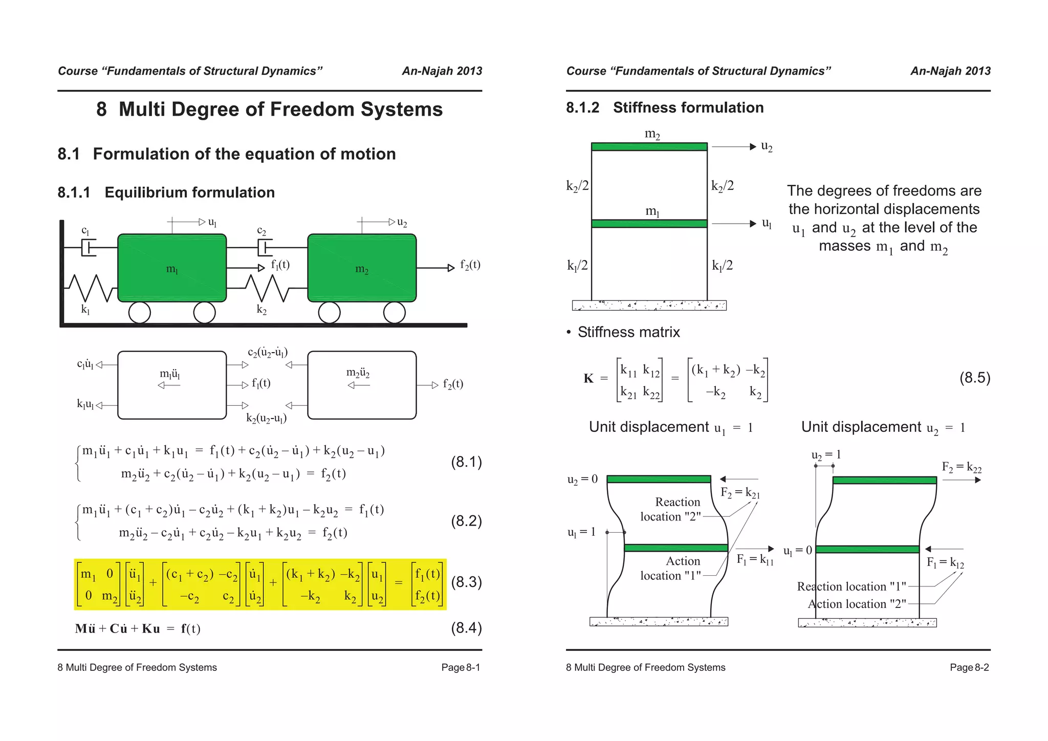
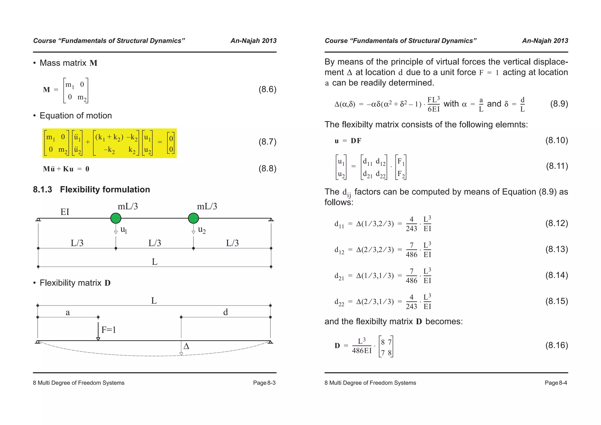
![Course “Fundamentals of Structural Dynamics” An-Najah 2013
8 Multi Degree of Freedom Systems Page8-5
• Stiffness matrix
(8.17)
• Mass matrix
(8.18)
• Equation of motion
(8.19)
(8.20)
8.1.4 Principle of virtual work
• See e.g. [Hum12]
8.1.5 Energie formulation
• See e.g. [Hum12]
K
K D 1– 162
5
---------
EI
L3
------ 8 7–
7– 8
⋅ ⋅= =
M
M
m1 0
0 m2
=
m1 0
0 m2
u··
1
u··
2
162
5
---------
EI
L3
------ 8 7–
7– 8
⋅ ⋅
u1
u2
+ 0
0
=
Mu·· Ku+ 0=
Course “Fundamentals of Structural Dynamics” An-Najah 2013
8 Multi Degree of Freedom Systems Page8-6
8.1.6 “Direct Stiffness Method”
• Stiffness matrix of a beam element
The stiffness matrix of a beam element with constant flexural
and axial stiffness is well known:
(8.21)
(8.22)
If the axial elongation of the beam is not considered, the matrix
can be further simplified as follows:
K
F Ku=
F1
F2
F3
F4
F5
F6
EA
L
-------- 0 0
EA
L
--------– 0 0
0
12EI
L3
------------
6EI
L2
--------- 0
12EI
L3
------------–
6EI
L2
---------
0
6EI
L2
---------
4EI
L
--------- 0
6EI
L2
---------–
2EI
L
---------
EA
L
--------– 0 0
EA
L
-------- 0 0
0
12EI
L3
------------–
6EI
L2
---------– 0
12EI
L3
------------
6EI
L2
---------–
0
6EI
L2
---------
2EI
L
--------- 0
6EI
L2
---------–
4EI
L
---------
u1
u2
u3
u4
u5
u6
⋅=](https://image.slidesharecdn.com/fundamentalsofstructuraldynamics-200730194708/75/Fundamentals-of-structural-dynamics-121-2048.jpg)
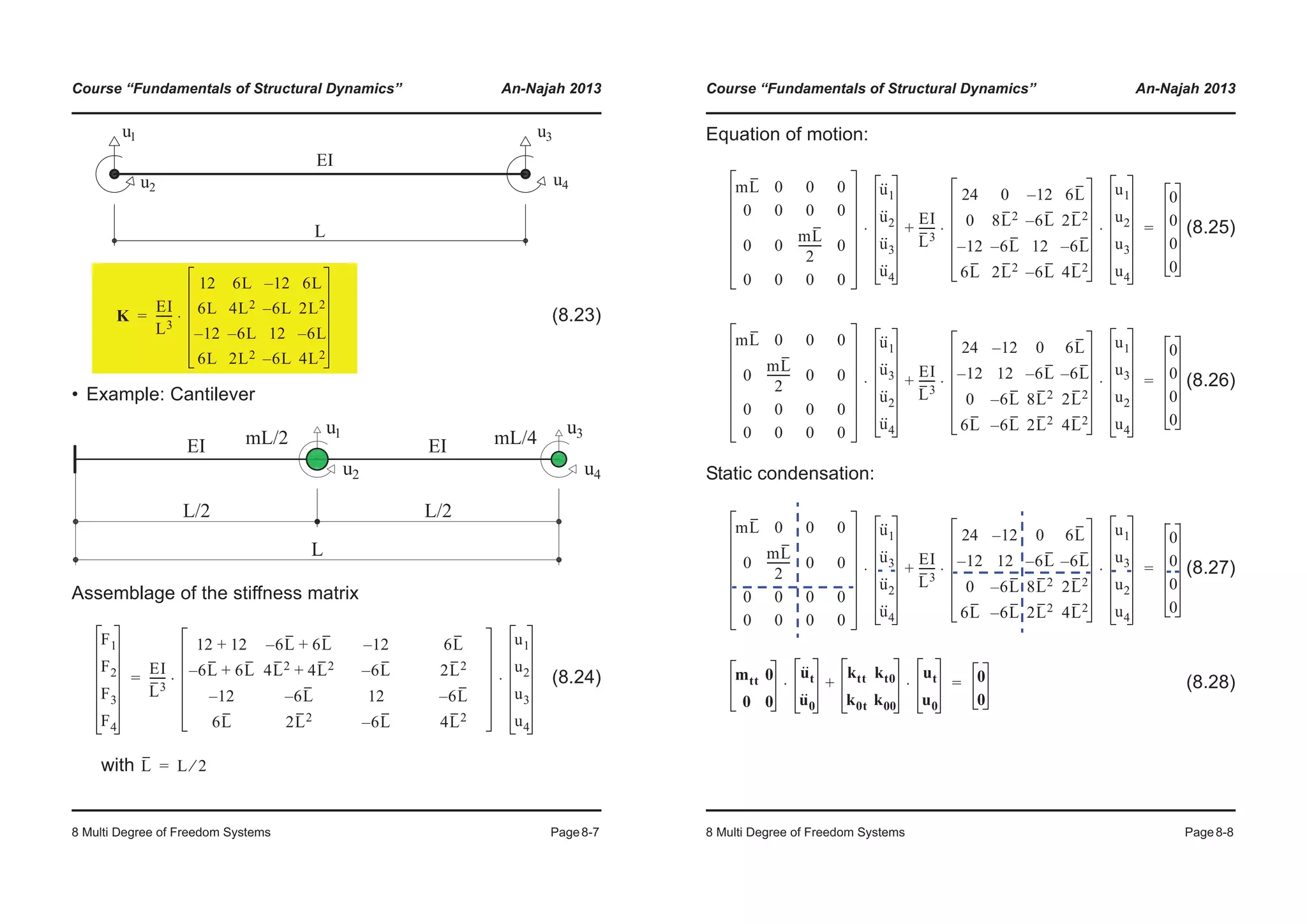
![Course “Fundamentals of Structural Dynamics” An-Najah 2013
8 Multi Degree of Freedom Systems Page8-9
(8.29)
From the second row of Equation (8.29) the following expression
can be derived:
(8.30)
Substituting Equation (8.30) in the first line of Equation (8.29) we
obtain:
(8.31)
(8.32)
and with :
(8.33)
with (8.34)
Where is the condensed stiffness matrix, and in our case it is
equal to:
(8.35)
mttu··
t kttut kt0u0+ + 0=
k0tut k00u0+ 0=¯
®
u0 k– 00
1–
k0tut=
mttu··
t kttut kt0k00
1–
k0tut–+ 0=
mttu··
t ktt kt0k00
1–
k0t–( )ut+ 0=
kt0 k0t
T
=
mttu··
t ktt k0t
T
k00
1–
k0t–( )ut+ 0=
mttu··
t kˆ ttut+ 0= kˆ
tt ktt k0t
T
k00
1–
k0t–=
kˆ
tt
kˆ
tt
EI
L3
------ 24 12–
12– 12
0 6L
6– L 6– L
1
7L2
---------
1
14L2
------------–
1
14L2
------------–
2
7L2
---------
0 6– L
6L 6– L
⋅ ⋅–
© ¹
¨ ¸
¨ ¸
¨ ¸
¨ ¸
§ ·
⋅=
Course “Fundamentals of Structural Dynamics” An-Najah 2013
8 Multi Degree of Freedom Systems Page8-10
(8.36)
after substituting :
(8.37)
The final equation of motion of the cantilever is therefore:
(8.38)
• Notes
• The “Direct Stiffness Method” is often used in the Finite Element
Method.
• The derivation of the stiffness matrix for a beam element and in-
structions for assembling the stiffness matrix of entire structures
can be found e.g. in the following references:
[Prz85] Przemieniecki J.S.: “Theory of Matrix Structural Analy-
sis”. Dover Publications, New York 1985.
[Bat96] Bathe K-J.: “Finite Element Procedures”. Prentice Hall,
Upper Saddle River, 1996.
kˆ
tt
EI
L3
------
6
7
--- 16 5–
5– 2
⋅ ⋅=
L L 2⁄=
kˆ
tt
EI
L3
------
48
7
------ 16 5–
5– 2
⋅ ⋅=
mL
2
-------- 0
0
mL
4
--------
u··
1
u··
3
⋅
EI
L3
------
48
7
------ 16 5–
5– 2
u1
u3
⋅ ⋅ ⋅+ 0
0
=
K](https://image.slidesharecdn.com/fundamentalsofstructuraldynamics-200730194708/75/Fundamentals-of-structural-dynamics-123-2048.jpg)
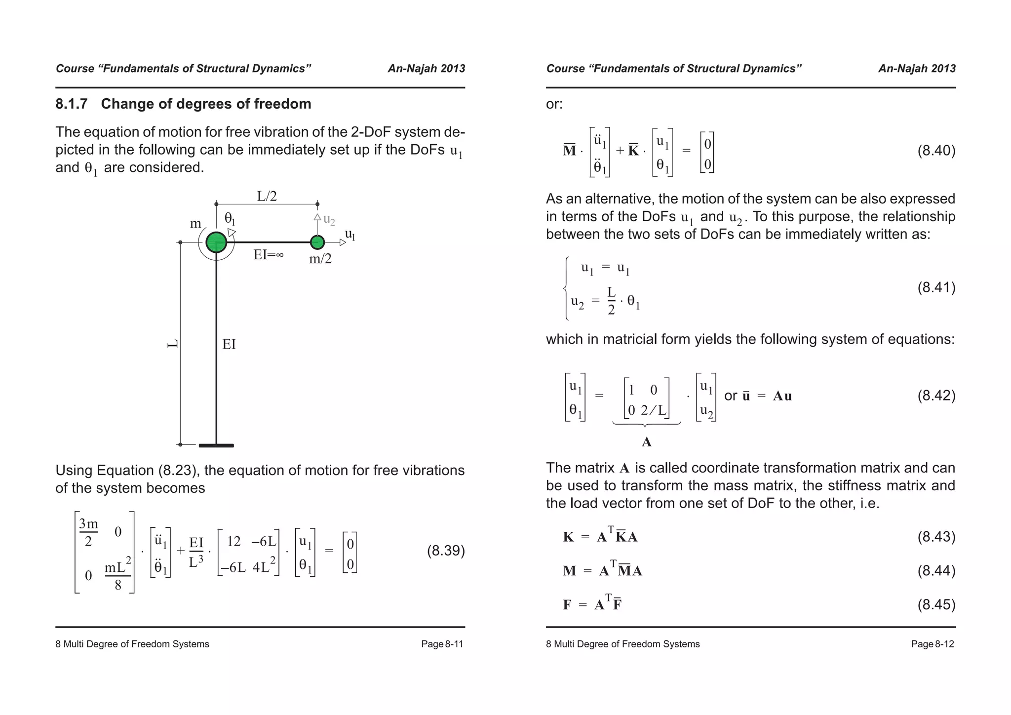
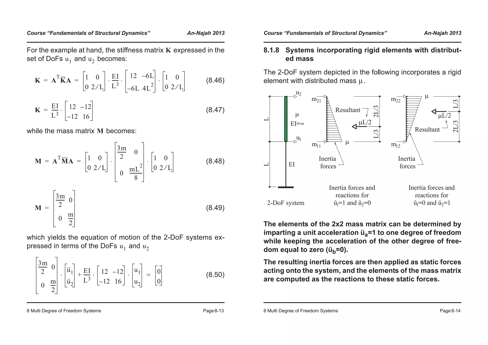
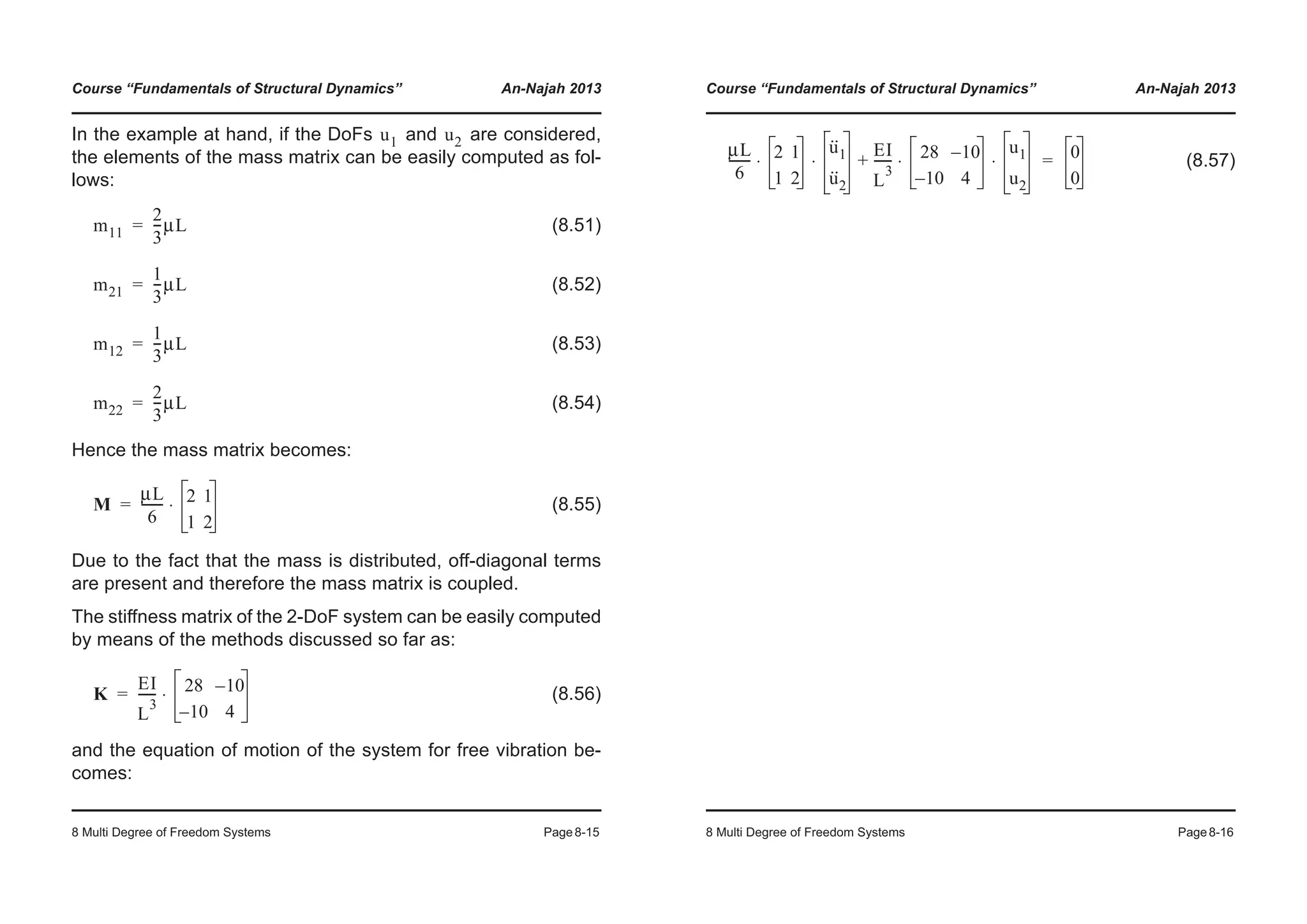
![Course “Fundamentals of Structural Dynamics” An-Najah 2013
9 Free Vibrations Page9-1
9 Free Vibrations
9.1 Natural vibrations
(9.1)
Ansatz:
where (9.2)
The double derivation of Equation (9.2) yields:
(9.3)
(9.4)
and by substituting Equations (9.2) and (9.4) in (9.1) we obtain:
(9.5)
Equation (9.5) is satisfied if , which is a trivial solution
meaning that there is no movement, because .
To obtain a nontrivial solution the term in brackets in Equation
(9.5) must be equal to zero, i.e.:
(9.6)
or:
with (9.7)
Mu·· Ku+ 0=
u t( ) qn t( )φφn= qn t( ) An ωnt( )cos Bn ωnt( )sin+=
q··
n t( ) ωn
2
An ωnt( )cos Bn ωnt( )sin+[ ]– ωn
2
qn t( )–= =
u·· t( ) ωn
2
qn t( )– φn=
ωn
2
Mφn– Kφn+[ ]qn t( ) 0=
qn t( ) 0=
u t( ) qn t( )φφn 0= =
ωn
2
M– K+[ ]φφn 0=
Aφn 0= A ωn
2
M– K+=
Course “Fundamentals of Structural Dynamics” An-Najah 2013
9 Free Vibrations Page9-2
Also in the case of Equation (9.7), there is always the trivial so-
lution , which corresponds to an absence of movement.
If the matrix has an inverse , then Equation (9.7) can be
rearranged as follows:
(9.8)
and therefore
(9.9)
This means that if matrix has an inverse , then Equations (9.6)
and (9.7) have only the trivial solution given by Equation (9.9).
The inverse of Matrix has the form:
(9.10)
If the determinant is equal to zero, then the matrix is singular
and has no inverse.
Therefore, Equation (9.6) has a nontrivial solution only if:
(9.11)
The determinant yields a polynomial of order in which is
called characteristic equation. The roots of the characteris-
tic equation are called eigenvalues and allow the calculation of
the natural circular frequencies of the system.
φn 0=
A A
1–
A
1–
Aφn A
1–
0=
φn 0=
A A
1–
A
A
1– 1
A
-------Aˆ=
A
ωn
2
M– K+ 0=
N ωn
2
N
N ωn](https://image.slidesharecdn.com/fundamentalsofstructuraldynamics-200730194708/75/Fundamentals-of-structural-dynamics-127-2048.jpg)
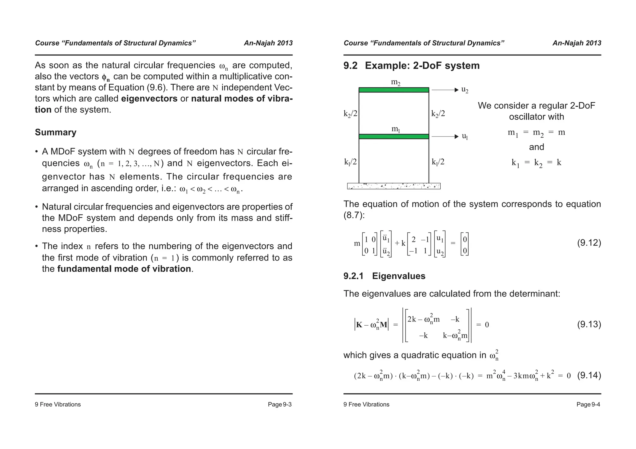
![Course “Fundamentals of Structural Dynamics” An-Najah 2013
9 Free Vibrations Page9-5
and both solutions yield the following eigenvalues:
(9.15)
For each eigenvalue we can now compute an eigenvector
and a natural circular frequency.
9.2.2 Fundamental mode of vibration
With the smallest eigenvalue we obtain the
1. circular frequency (9.16)
By substituting this eigenvalue into the system of equations
(9.17)
we obtain two independent equations that can be used to deter-
mine the elements of the first eigenvector . The first row of the
system yield the equation:
and (9.18)
and by substituting this into the second row we obtain:
ωn
2 3km 9k
2
m
2
4k
2
m
2
–±
2m
2
------------------------------------------------------------
3 5±
2
----------------
k
m
----⋅= =
ωn
2
ω1
2 3 5–
2
----------------
k
m
----⋅=
ω1
3 5–
2
----------------
k
m
----⋅ 0.618
k
m
----= =
ω1
2
K ω1
2
M–[ ]φφ1
2k
3 5–
2
----------------
k
m
----⋅
© ¹
§ · m– k–
k– k
3 5–
2
----------------
k
m
----⋅
© ¹
§ · m–
φ11
φ21
⋅ 0
0
= =
φ1
1 5+( )k
2
------------------------φ11 kφ21– 0= φ21
1 5+( )
2
---------------------φ11=
Course “Fundamentals of Structural Dynamics” An-Najah 2013
9 Free Vibrations Page9-6
(9.19)
As expected, the eigenvector is determined within a multiplica-
tive constant, and can therefore be arbitrarily normalized as fol-
lows:
• so that the largest element of the eigenvector is equal to 1
• so that one particular element of the eigenvector is equal to 1
• so that the norm of the eigenvector is equal to 1
• ...
Fundamental mode:
kφ11–
1– 5+( )k
2
-----------------------------
1 5+( )
2
---------------------φ11© ¹
§ ·+ 0
kφ11– kφ11+ 0
φ11 φ11
=
=
=
“Degree of freedom”
“Mode”
ω1
3 5–
2
----------------
k
m
----⋅ 0.618
k
m
----= =
φ1
φ11
φ21
2
1 5+
----------------
1
0.618
1
= = =](https://image.slidesharecdn.com/fundamentalsofstructuraldynamics-200730194708/75/Fundamentals-of-structural-dynamics-129-2048.jpg)
![Course “Fundamentals of Structural Dynamics” An-Najah 2013
9 Free Vibrations Page9-7
9.2.3 Higher modes of vibration
Additionally to the fundamental mode of vibration, the consid-
ered 2-DoF system has a second mode of vibration.
The properties of this second mode of vibration can be comput-
ed in analogy to the fundamental mode and the following results
are obtained:
Second mode
“Degree of freedom”
“Mode”
ω2
3 5+
2
----------------
k
m
----⋅ 1.618
k
m
----= =
φ2
φ12
φ22
1
1 5–
2
----------------
1
0.618–
= = =
Course “Fundamentals of Structural Dynamics” An-Najah 2013
9 Free Vibrations Page9-8
9.2.4 Free vibrations of the 2-DoF system
According to Equation (9.2), the free vibration of the 2-DoF sys-
tem is:
(9.20)
(9.21)
The still unknown constants to can be computed using the
initial conditions given by Equation (9.24) and become:
, (9.22)
, (9.23)
Initial conditions: (9.24)
For an alternative methodology to compute the constants to
see Section 9.6.
u C1 ω1t( )cos C2 ω1t( )sin+[ ]φφ1 C3 ω2t( )cos C4 ω2t( )sin+[ ]φφ2+=
u1
u2
C1 ω1t( )cos C2 ω1t( )sin+[ ]
φ11
φ21
C3 ω2t( )cos C4 ω2t( )sin+[ ]
φ12
φ22
+
=
C1 C4
C1
φ22u1 φ12u2–
φ11φ22
φ21φ12
–
--------------------------------------= C2
φ22v1 φ12v2–
φ11φ22
φ21φ12
–( )ω1
-------------------------------------------------=
C3
φ11u2 φ21u1–
φ11φ22
φ21φ12
–
--------------------------------------= C4
φ11v2 φ21v1–
φ11φ22
φ21φ12
–( )ω2
-------------------------------------------------=
u1 0( ) u1=
u2 0( ) u2=
u·
1 0( ) v1=
u·
2 0( ) v2=¯
°
°
®
°
°
C1
C4](https://image.slidesharecdn.com/fundamentalsofstructuraldynamics-200730194708/75/Fundamentals-of-structural-dynamics-130-2048.jpg)
![Course “Fundamentals of Structural Dynamics” An-Najah 2013
9 Free Vibrations Page9-9
• Case 1: , ,u1 0.618= u2 1.000= v1 v2 0= =
-0.4
-0.2
0.0
0.2
0.4
0.6
0.8
1.0
1.2
splacementu2[m]
First mode
Second mode
Total displacement
-1.2
-1.0
-0.8
-0.6
0 5 10 15 20
Dis
Time [s]
-0.4
-0.2
0.0
0.2
0.4
0.6
0.8
1.0
1.2
splacementu1[m]
First mode
Second mode
Total displacement
-1.2
-1.0
-0.8
-0.6
0 5 10 15 20
Dis
Time [s]
Course “Fundamentals of Structural Dynamics” An-Najah 2013
9 Free Vibrations Page9-10
• Case 2: , ,u1 1.000= u2 0.618–= v1 v2 0= =
-0.4
-0.2
0.0
0.2
0.4
0.6
0.8
1.0
1.2
splacementu2[m]
First mode
Second mode
Total displacement
-1.2
-1.0
-0.8
-0.6
0 5 10 15 20
Dis
Time [s]
-0.4
-0.2
0.0
0.2
0.4
0.6
0.8
1.0
1.2
splacementu1[m]
First mode
Second mode
Total displacement
-1.2
-1.0
-0.8
-0.6
0 5 10 15 20
Dis
Time [s]](https://image.slidesharecdn.com/fundamentalsofstructuraldynamics-200730194708/75/Fundamentals-of-structural-dynamics-131-2048.jpg)
![Course “Fundamentals of Structural Dynamics” An-Najah 2013
9 Free Vibrations Page9-11
• Case 3: , ,u1 0.618= u2 0.000= v1 v2 0= =
-0.2
0.0
0.2
0.4
0.6
0.8
splacementu2[m]
First mode
Second mode
Total displacement
-0.8
-0.6
-0.4
0 5 10 15 20
Dis
Time [s]
-0.2
0.0
0.2
0.4
0.6
0.8
splacementu1[m]
First mode
Second mode
Total displacement
-0.8
-0.6
-0.4
0 5 10 15 20
Dis
Time [s]
Course “Fundamentals of Structural Dynamics” An-Najah 2013
9 Free Vibrations Page9-12
9.3 Modal matrix and Spectral matrix
All eigenvalues and all eigenvectors can be compactly rep-
resented in matricial form:
• Modal matrix
(9.25)
• Spectral matrix
(9.26)
Equation (9.6) can therefore be rearranged as follows:
(9.27)
and it is immediately apparent that the equation for all eigenval-
ues and all eigenvectors can be expressed in terms of modal
and the spectral matrices, as follows:
(9.28)
N N
Φ φjn[ ]
φ11 φ12 … φ1N
φ21 φ22 … φ2N
… … … …
φN1 φN2 … φNN
= =
Ω
2
ω1
2 0 … 0
0 ω2
2 … 0
… … … …
0 0 … ωN
2
=
Kφn Mφnωn
2=
KΦ MΦΩ
2
=](https://image.slidesharecdn.com/fundamentalsofstructuraldynamics-200730194708/75/Fundamentals-of-structural-dynamics-132-2048.jpg)
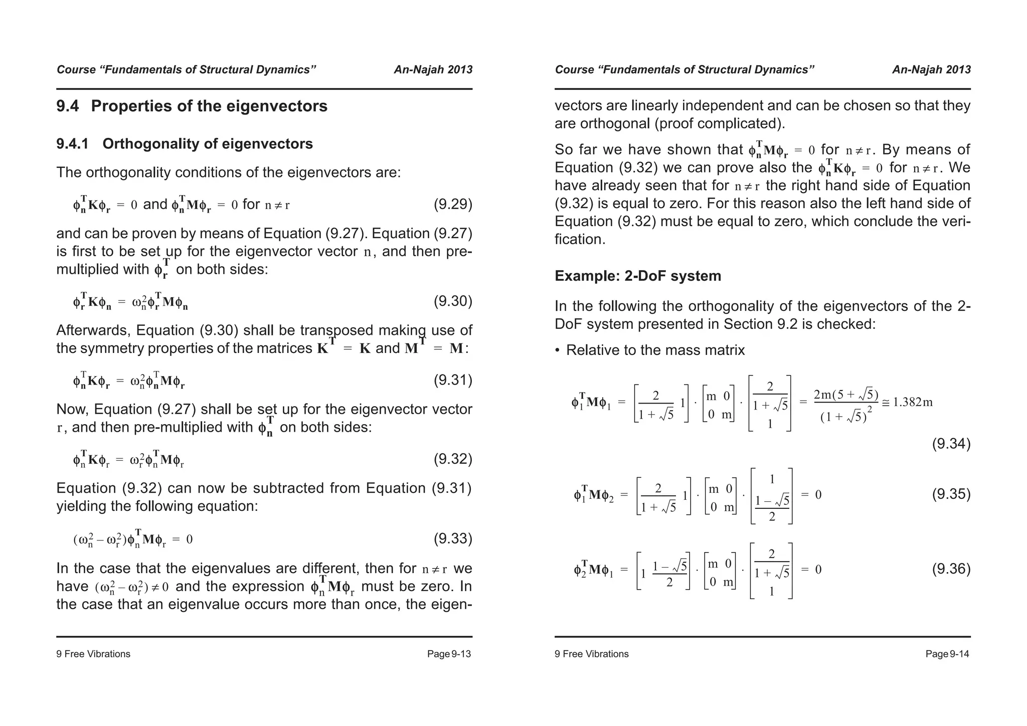
![Course “Fundamentals of Structural Dynamics” An-Najah 2013
9 Free Vibrations Page9-21
• Second modal SDoF system:
(9.68)
(9.69)
(9.70)
The natural frequency corresponds to the result shown on page
9-7.
m2
*q··
2 t( ) k2
*q2 t( )+ 0=
1.382mq··
2 t( ) 3.618kq2 t( )+ 0=
ω2
k2
*
m2
*
-------
3.618k
1.382m
------------------ 1.618
k
m
----= = =
Course “Fundamentals of Structural Dynamics” An-Najah 2013
9 Free Vibrations Page9-22
9.6 Free vibration response
9.6.1 Systems without damping
The equation of motion for free vibration of a system without
damping is
(9.71)
and making use of the possibility of decoupling of the equation
of motion, the total deformation under free vibration can be
computed as the sum of the contribution of all modes. The equa-
tion of motion of the nth
decoupled SDoF system is:
(9.72)
and its solution can be computed as discussed in Chapter 3 for
SDoF systems. If we make use of the second formulation with
“trigonometric functions” (see Section 3.1.2), the solution is:
(9.73)
The the total deformation under free vibration is hence
(9.74)
The constants and can be computed by means of the
initial conditions and .
To this purpose, the vector of the velocity is needed and can
easily be computed by deriving Equation (9.74), i.e.:
Mu·· Ku+ 0=
u t( )
mn
*q··
n t( ) kn
*qn t( )+ 0=
qn t( ) An ωnt( )cos Bn ωnt( )sin+=
u t( )
u t( ) φφiqi
t( )
i 1=
N
¦ φi Ai ωit( )cos Bi ωit( )sin+[ ]
i 1=
N
¦= =
2 N⋅ Ai Bi
u 0( ) u0= u· 0( ) v0=](https://image.slidesharecdn.com/fundamentalsofstructuraldynamics-200730194708/75/Fundamentals-of-structural-dynamics-137-2048.jpg)
![Course “Fundamentals of Structural Dynamics” An-Najah 2013
9 Free Vibrations Page9-23
(9.75)
Considering Equations (9.74) and (9.75) at the time , we
have.
and (9.76)
Making use of Equation (9.59) we can now write the equations
to compute the initial conditions of the nth
decoupled SDoF sys-
tem as:
(9.77)
(9.78)
In Section 3.1.2 (see Equation 3.18) it as been shown that the
constants and are equal to and , respec-
tively, hence Equation (9.74) can be rewritten as:
(9.79)
u· t( ) φφiq·
i
t( )
i 1=
N
¦ φiωi A– i ωit( )sin Bi ωit( )cos+[ ]
i 1=
N
¦= =
t 0=
u 0( ) φφiqi
0( )
i 1=
N
¦= u· 0( ) φφiq·
i
0( )
i 1=
N
¦=
qn 0( )
φn
T
Mu 0( )
φn
T
Mφn
------------------------=
q·
n 0( )
φn
T
Mu· 0( )
φn
T
Mφn
------------------------=
An Bn qn 0( ) q·
n 0( ) ωn⁄
u t( ) φφi qi 0( ) ωit( )cos
q·
i 0( )
ωi
------------ ωit( )sin+
i 1=
N
¦=
Course “Fundamentals of Structural Dynamics” An-Najah 2013
9 Free Vibrations Page9-24
9.6.2 Classically damped systems
The equation of motion for free vibration of a system with damp-
ing is
(9.80)
As it will be shown in Chapter 10, if the MDoF system is classi-
cally damped, the equation of motion can be decoupled analo-
gously to system without damping, and the total deformation
under free vibration can be computed again as the sum of the
contribution of all modes. The equation of motion of the nth de-
coupled SDoF system is:
(9.81)
or
(9.82)
where
and , respectively. (9.83)
The solution of Equation (9.82) can be computed as discussed
in Chapter 3 for SDoF systems. According to Equation (3.50) we
have:
(9.84)
where:
Mu·· Cu·+ Ku+ 0=
u t( )
mn
*q··
n t( ) cn
*q·
n t( ) kn
*qn t( )+ + 0=
q··
n t( ) 2ωnζnqn
t( ) ωn
2
qn t( )+ + 0=
cn
* φn
T
Cφn= ζn
cn
*
2mn
*ωn
-----------------=
qn t( ) e
ζωnt–
An ωndt( )cos Bn ωndt( )sin+[ ]=](https://image.slidesharecdn.com/fundamentalsofstructuraldynamics-200730194708/75/Fundamentals-of-structural-dynamics-138-2048.jpg)
![Course “Fundamentals of Structural Dynamics” An-Najah 2013
9 Free Vibrations Page9-25
“damped circular frequency of the nth mode”
(9.85)
The the total deformation under free vibration is hence
(9.86)
As in the case of the undamped systems, the constants
and can be computed by means of the initial conditions
and .
For the nth decoupled SDoF system according to Equation (3.51)
the constants and can be expressed in function of the in-
itial conditions of the modal coordinate as follows:
(9.87)
(9.88)
where the initial displacement and the initial velocity
can be computed by means of Equations (9.77) and (9.78).
Hence, the total displacement of a classically damped MDoF
system under free vibration can be computed as:
(9.89)
For nonclassically damped system see e.g. [Cho11], Chapter 14.
ωnd ωn 1 ζ
2
–=
u t( )
u t( ) φφiqi
t( )
i 1=
N
¦ φie
ζωnt–
Ai ωidt( )cos Bi ωidt( )sin+[ ]
i 1=
N
¦= =
2 N⋅ Ai
Bi
u 0( ) u0= u· 0( ) v0=
An Bn
q
An qn 0( )=
Bn
q·
n 0( ) ζωnqn 0( )+
ωnd
--------------------------------------------=
qn 0( ) q·
n 0( )
u t( ) φφie
ζωnt–
qi 0( ) ωidt( )cos
q·
i 0( ) ζωiqi 0( )+
ωid
----------------------------------------- ωidt( )sin+
i 1=
N
¦=
Course “Fundamentals of Structural Dynamics” An-Najah 2013
9 Free Vibrations Page9-26
Blank Page](https://image.slidesharecdn.com/fundamentalsofstructuraldynamics-200730194708/75/Fundamentals-of-structural-dynamics-139-2048.jpg)
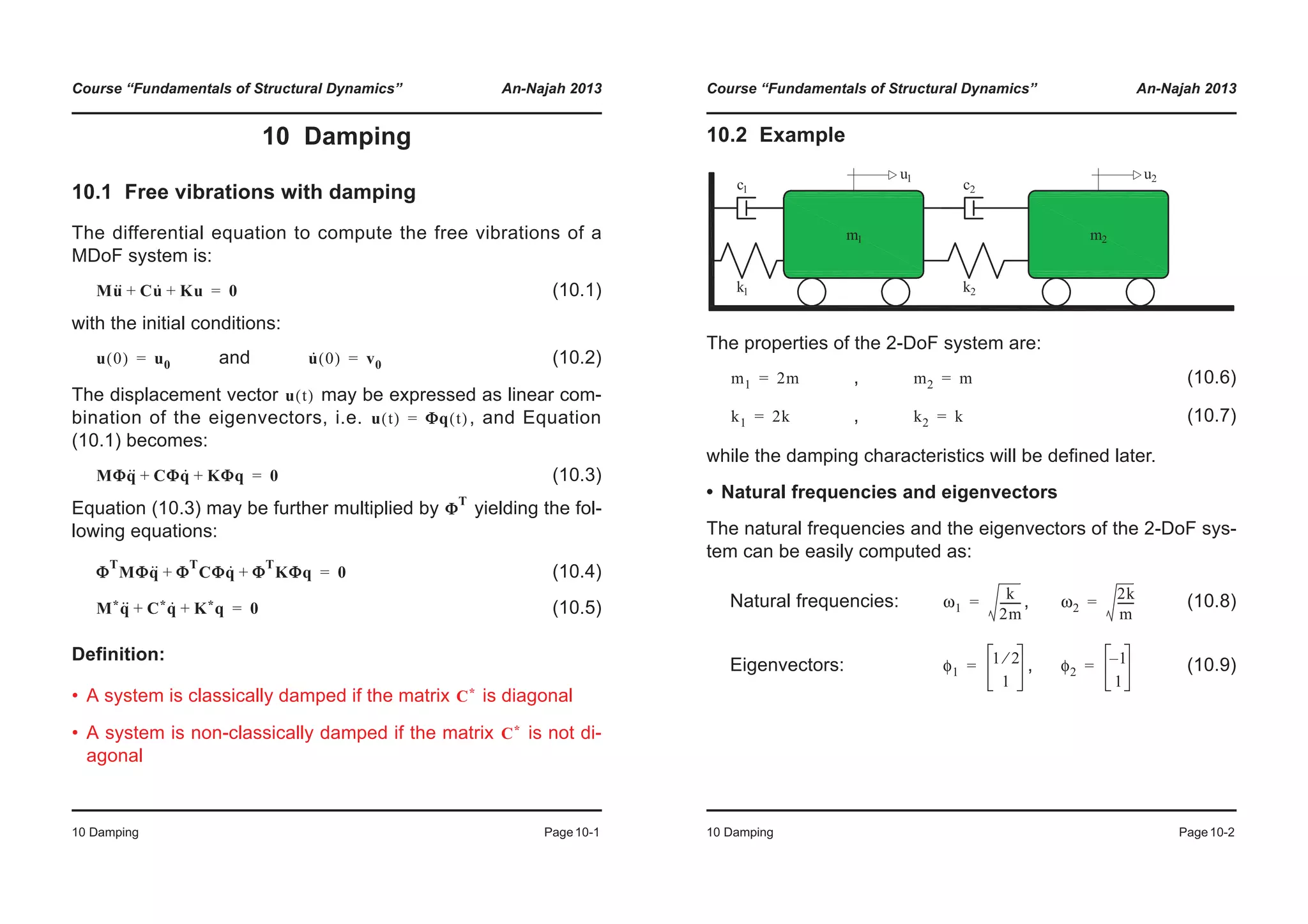
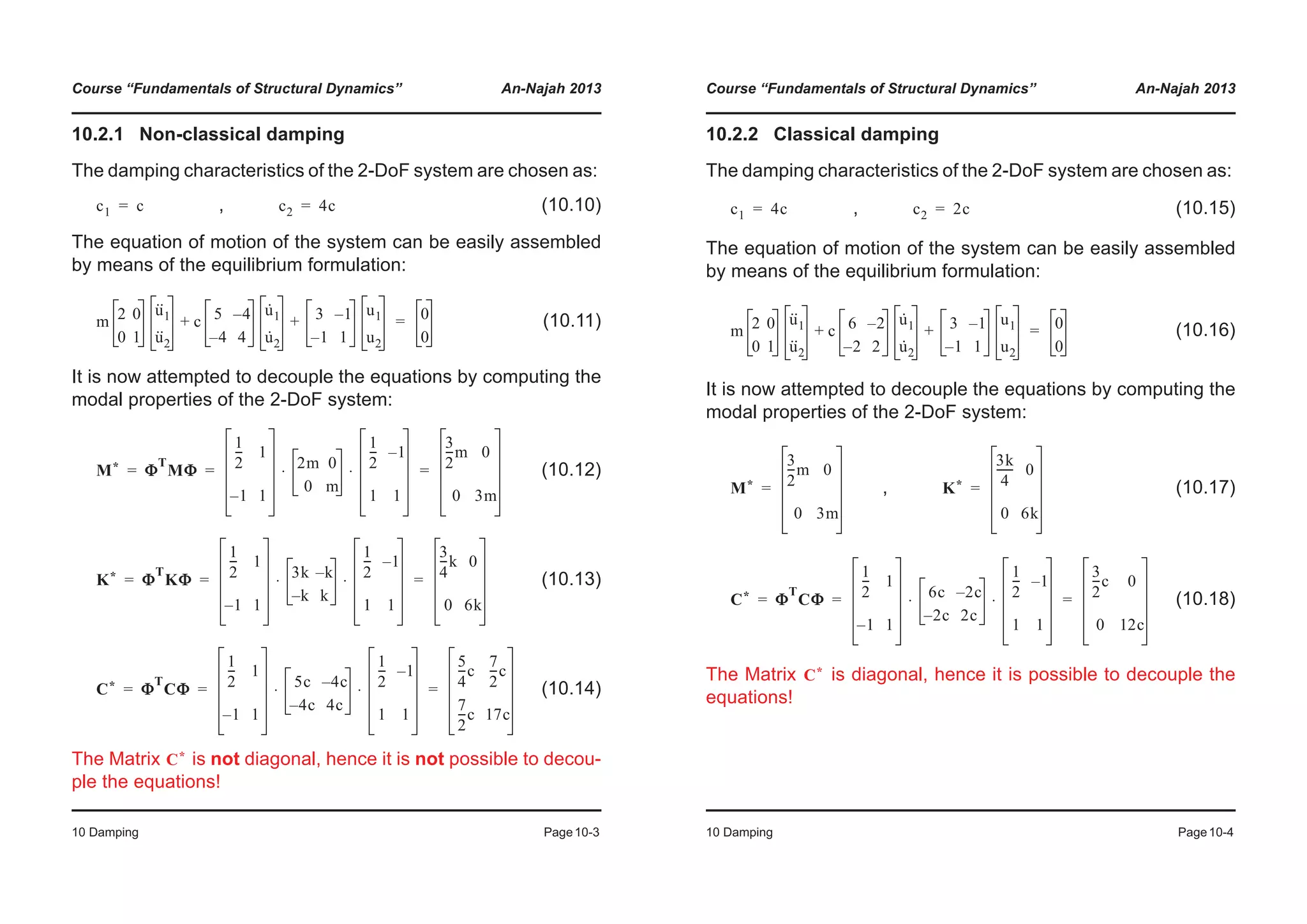
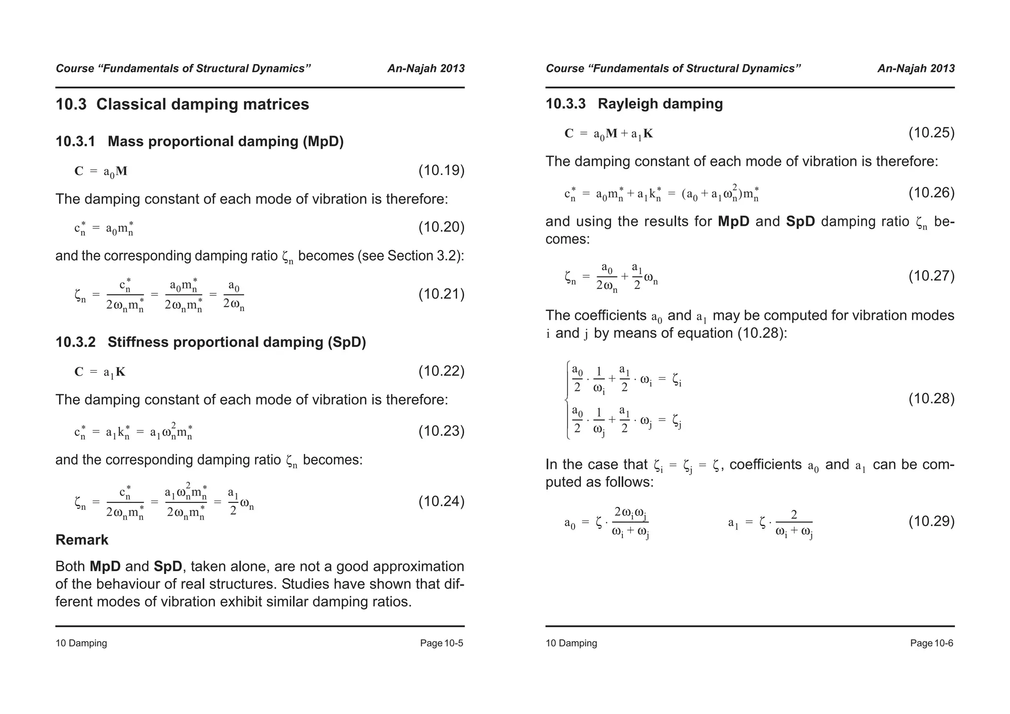
![Course “Fundamentals of Structural Dynamics” An-Najah 2013
10 Damping Page10-7
10.3.4 Example
A damping matrix shall be assembled so that in the case of the
2-DoF system shown on page 10-2 both modes of vibration are
characterised by the same damping ratio .
The natural frequencies are:
, (10.30)
hence the coefficients and become:
, (10.31)
yielding the damping matrix equal to:
(10.32)
Check:
(10.33)
The damping matrix is indeed diagonal.
ζ
ω1
k
2m
--------= ω2
2k
m
------=
a0 a1
a0
4ζ
3
------ m
2k
------
k
m
----⋅ ⋅= a1
4ζ
3
------ m
2k
------⋅=
C a0M a1K+=
C
4ζ
3
------ m
2k
------
k
m
---- 2m 3k+⋅ 0 k–
0 k–
k
m
---- m k+⋅
⋅ ⋅
4ζ
3
------ mk
2
-------- 5 1–
1– 2
⋅ ⋅= =
C* Φ
T
CΦ
1
2
--- 1
1– 1
4ζ
3
------ mk
2
-------- 5 1–
1– 2
1
2
--- 1–
1 1
⋅ ⋅ ⋅ ⋅ ζ
mk
2
-------- 3 0
0 12
⋅ ⋅= = =
Course “Fundamentals of Structural Dynamics” An-Najah 2013
10 Damping Page10-8
If we choose values for , and so that
, , (10.34)
the coefficients and become:
, (10.35)
and the representation of the damping ratio in function of the nat-
ural circular frequency is:
Remarks
- If there are more than 2 modes of vibrations, then not all of
them will have the same damping ratio.
- If more than 2 modes of vibrations should have the same
damping, then a different damping modal shall be used. To
this purpose see e.g. “Caughey-Damping” in [Cho11].
m k ζ
ω1 2rad s⁄= ω2 5rad s⁄= ζ 5%=
a0 a1
a0 14.287= a1 1.429=
4
5
6
7
8
9
10
mpingratioζn[%]
Mass proportional damping
Stiffness proportional damping
Rayleigh Damping
0
1
2
3
0 1 2 3 4 5 6 7 8 9 10
Dam
Circular frequency ω](https://image.slidesharecdn.com/fundamentalsofstructuraldynamics-200730194708/75/Fundamentals-of-structural-dynamics-143-2048.jpg)
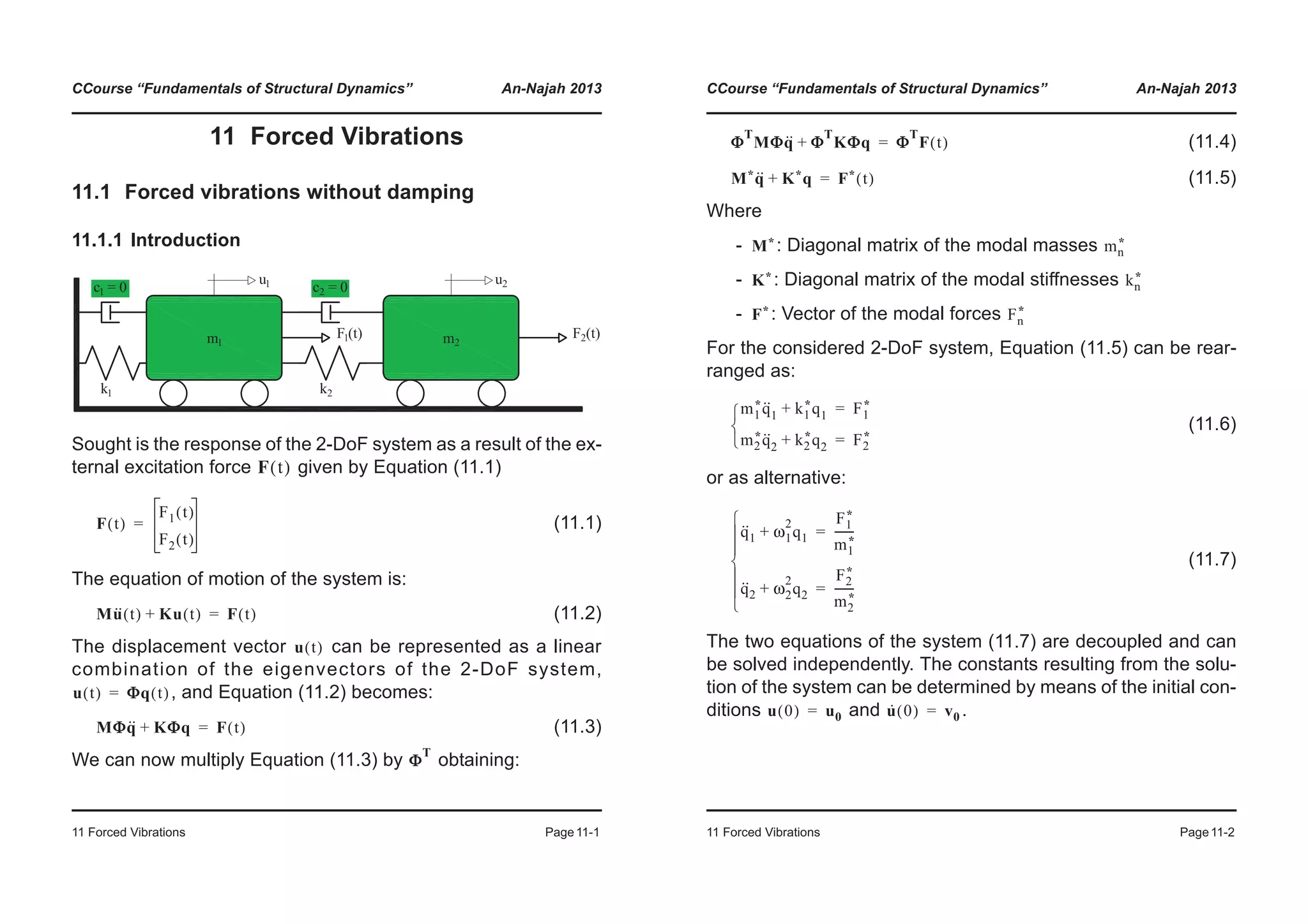
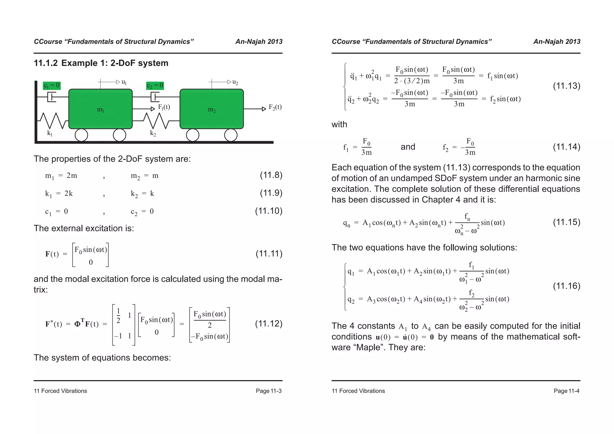
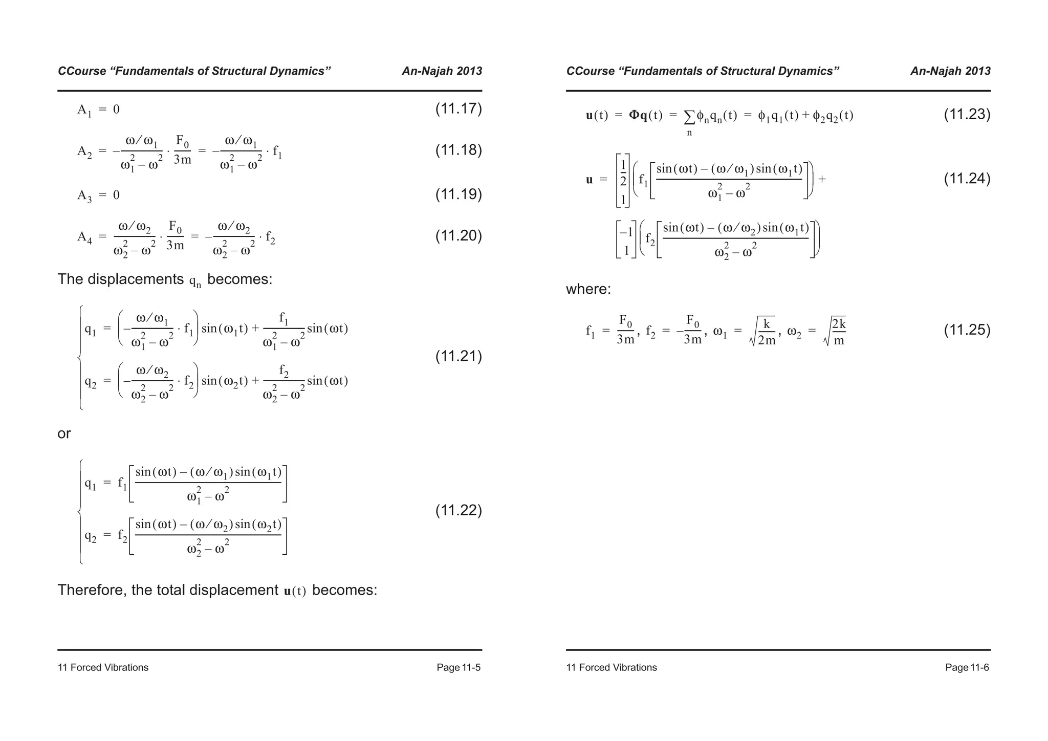
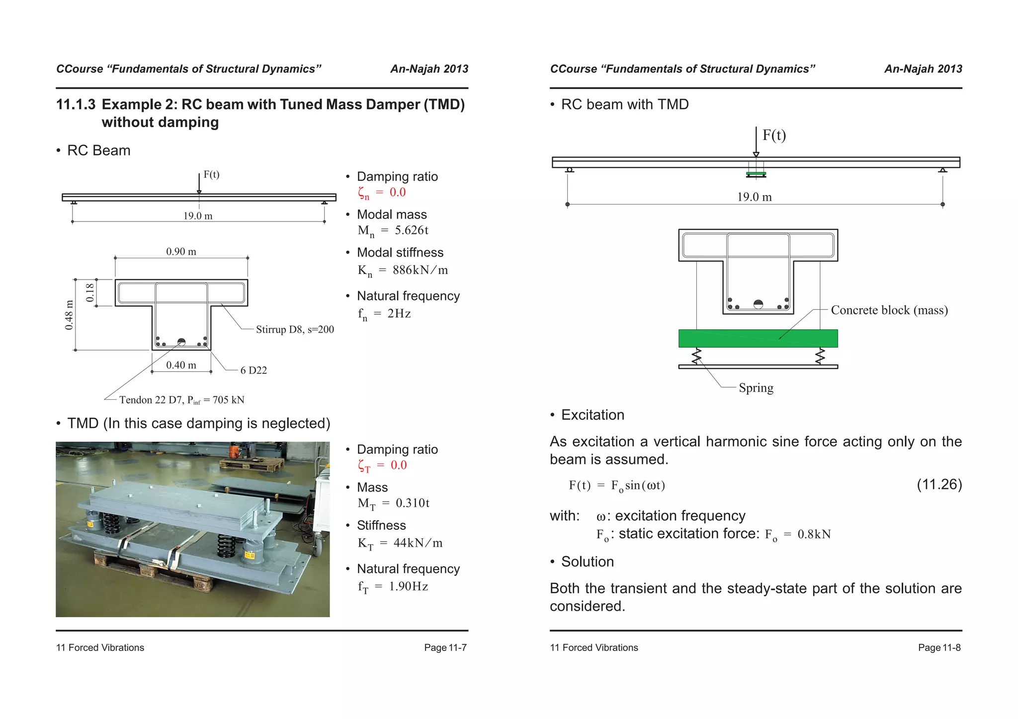
![CCourse “Fundamentals of Structural Dynamics” An-Najah 2013
11 Forced Vibrations Page11-9
• Case 1: , excitation frequencyKT 10000kN m⁄= f 2Hz=
-0.01
0
0.01
0.02
0.03
0.04
placementu1(t)[m]
Displacement of the beam
-0.04
-0.03
-0.02
0 1 2 3 4 5 6 7 8 9 10 11 12 13 14 15 16 17 18 19 20
Disp
Time [s]
-0.01
0
0.01
0.02
0.03
0.04
splacementu2[m]
Displacement of the TMD
-0.04
-0.03
-0.02
0 1 2 3 4 5 6 7 8 9 10 11 12 13 14 15 16 17 18 19 20
Dis
Time [s]
CCourse “Fundamentals of Structural Dynamics” An-Najah 2013
11 Forced Vibrations Page11-10
• Remarks
- The amplification factor is defined as:
,
where
- The solution was computed by means of the Excel file giv-
en on the web page of the course (SD_MDOF_TMD.xlsx)
- The Tuned Mass Damper (TMD) is blocked
- The natural frequency of the beam with TMD is:
- At resonance occurs. In the diagram above the am-
plification factor is limited, because the response of the
system was only calculated during 60 seconds.
60
80
100
120
140
plificationfactorA[-]
Displacement of the beam (u1)
Displacement of the TMD (u2)
0
20
40
0.5 0.6 0.7 0.8 0.9 1 1.1 1.2 1.3 1.4 1.5
Amp
Excitation frequency / Natural frequency of the beam [-]
A
ATMD u2 ust⁄= ABeam u1 ust⁄=
ust Fo Kn⁄=
fn 1.94Hz=
f fn=](https://image.slidesharecdn.com/fundamentalsofstructuraldynamics-200730194708/75/Fundamentals-of-structural-dynamics-148-2048.jpg)
![CCourse “Fundamentals of Structural Dynamics” An-Najah 2013
11 Forced Vibrations Page11-11
• Case 2: , excitation frequencyKT 44kN m⁄= f 2Hz=
-0.002
0
0.002
0.004
0.006
0.008
placementu1(t)[m]
Displacement of the beam
-0.008
-0.006
-0.004
0 1 2 3 4 5 6 7 8 9 10 11 12 13 14 15 16 17 18 19 20
Disp
Time [s]
-0.01
0
0.01
0.02
0.03
0.04
splacementu2[m]
Displacement of the TMD
-0.04
-0.03
-0.02
0 1 2 3 4 5 6 7 8 9 10 11 12 13 14 15 16 17 18 19 20
Dis
Time [s]
CCourse “Fundamentals of Structural Dynamics” An-Najah 2013
11 Forced Vibrations Page11-12
• Remarks
- The amplification factor is defined as:
,
where
- The solution was computed by means of the Excel file giv-
en on the web page of the course (SD_MDOF_TMD.xlsx)
- The Tuned Mass Damper (TMD) is free to move
- No resonance at occurs. Resonance occurs in corre-
spondence of the first and of the second natural frequen-
cies of the 2-DoF system.
In the diagram above the factor is limited, because the
response of the system was only calculated during 60s.
150
200
250
300
350
plificationfactorA[-]
Displacement of the beam (u1)
Displacement of the TMD (u2)
0
50
100
0.5 0.6 0.7 0.8 0.9 1 1.1 1.2 1.3 1.4 1.5
Amp
Excitation frequency / Natural frequency of the beam [-]
A
ATMD u2 ust⁄= ABeam u1 ust⁄=
ust Fo Kn⁄=
f fn=
A](https://image.slidesharecdn.com/fundamentalsofstructuraldynamics-200730194708/75/Fundamentals-of-structural-dynamics-149-2048.jpg)
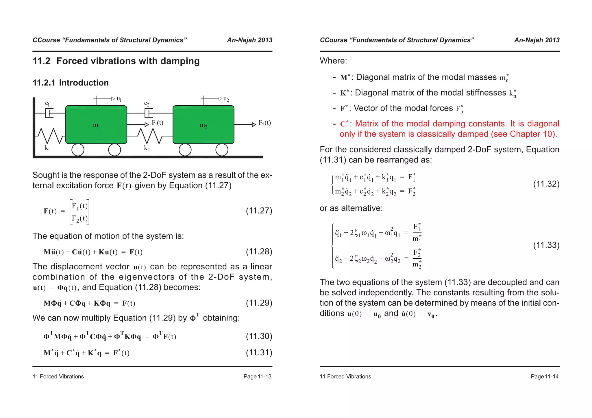
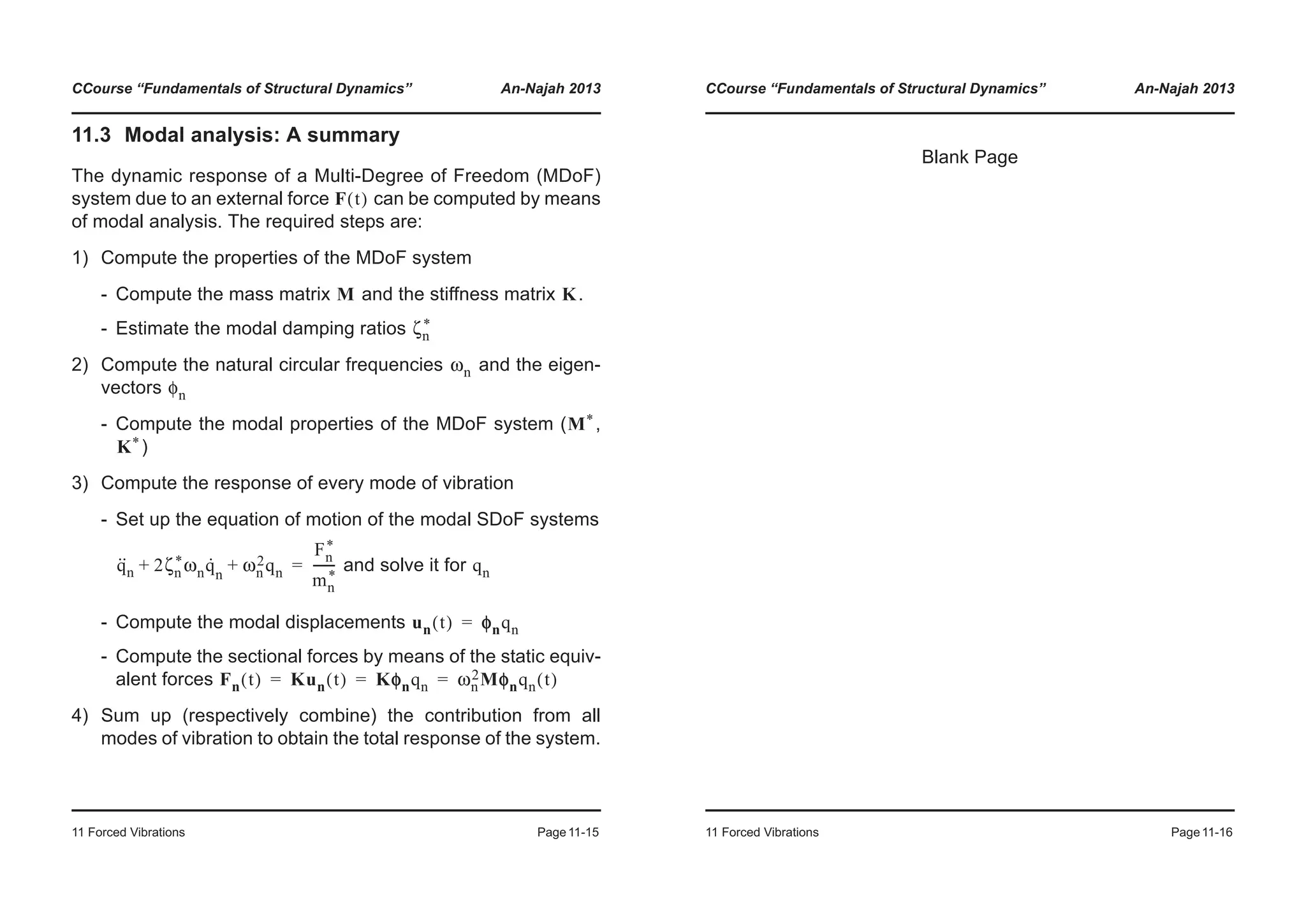
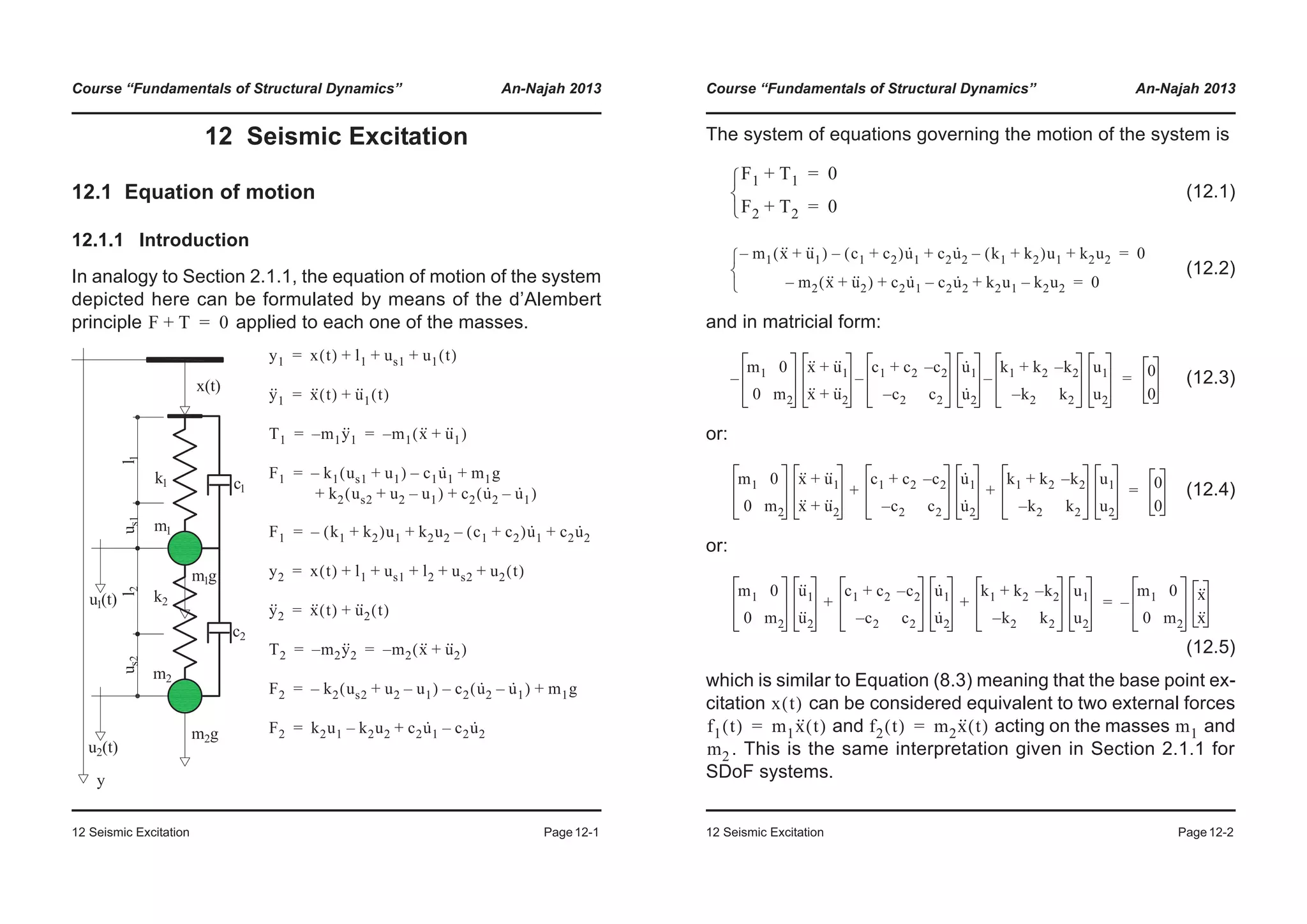
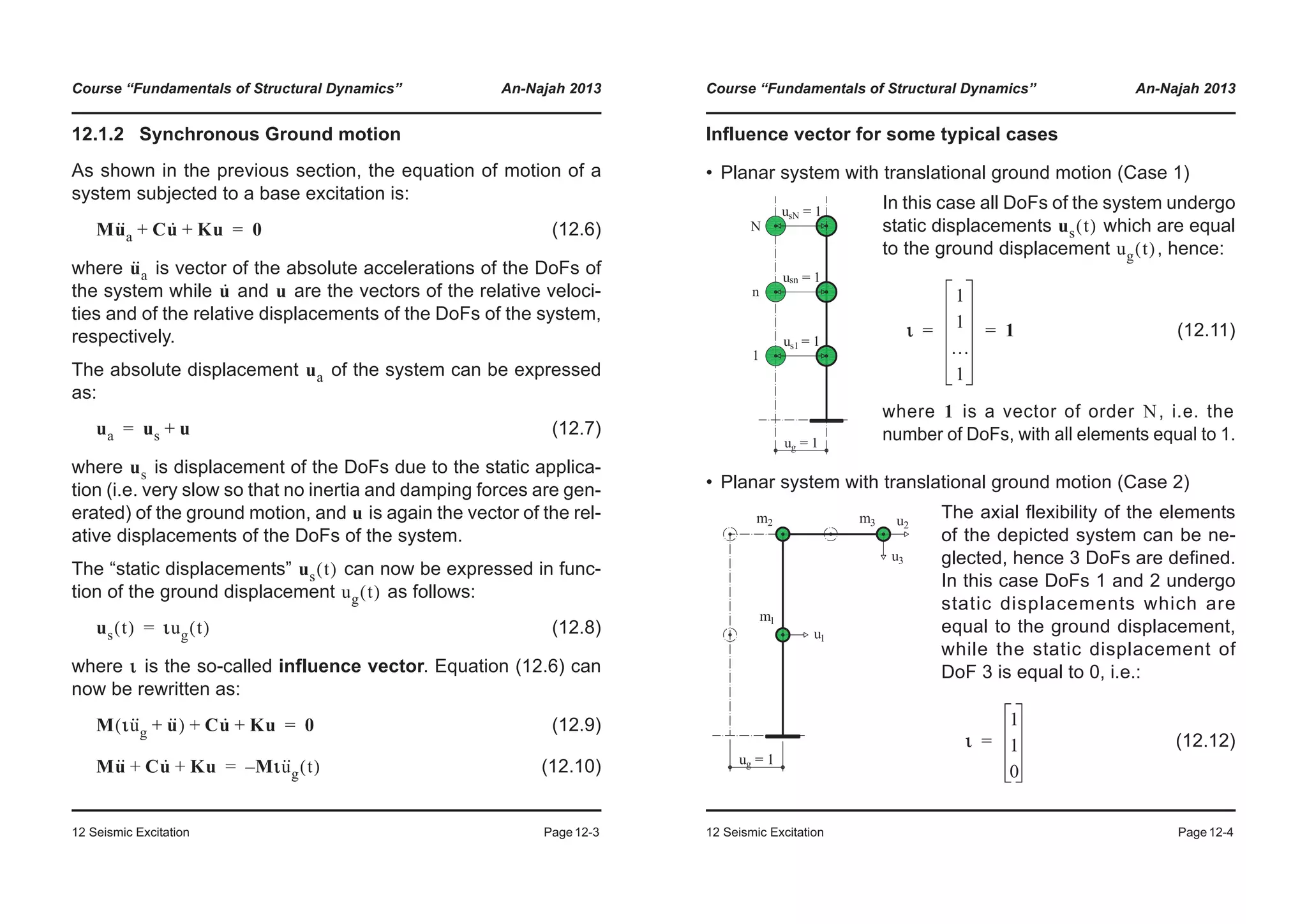
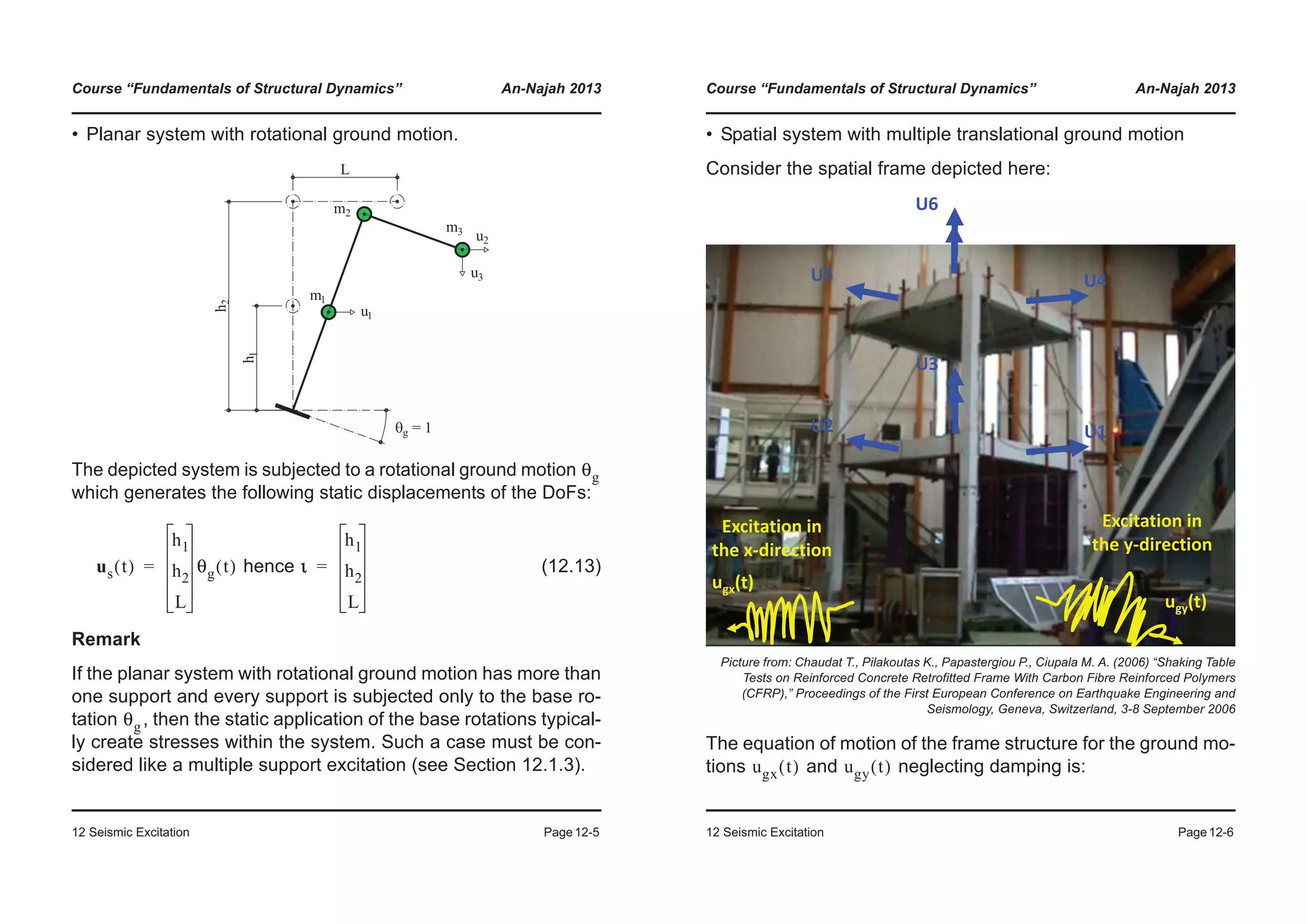
![Course “Fundamentals of Structural Dynamics” An-Najah 2013
12 Seismic Excitation Page12-7
(12.14)
(12.15)
and with
we obtain
(12.16)
Remarks
• For other cases see [Cho11] Sections 9.4 to 9.6.
M
u··
1
u··
2
u··
3
u··
4
u··
5
u··
6
K
u1
u2
u3
u4
u5
u6
+ Mιxu··
gx
t( ) Mιyu··
gy
t( )––=
M
u··
1
u··
2
u··
3
u··
4
u··
5
u··
6
K
u1
u2
u3
u4
u5
u6
+ M
0
1
0
0
1
0
u··
gx t( )
1
0
0
1
0
0
u··
gy t( )+
© ¹
¨ ¸
¨ ¸
¨ ¸
¨ ¸
¨ ¸
¨ ¸
¨ ¸
§ ·
–=
M
m1
m2 0
I3
m4
0 m5
I6
= M
u··
1
u··
2
u··
3
u··
4
u··
5
u··
6
K
u1
u2
u3
u4
u5
u6
+
m1u··
gy–
m2u··
gx–
0
m4u··
gy–
m5u··
gx–
0
=
Course “Fundamentals of Structural Dynamics” An-Najah 2013
12 Seismic Excitation Page12-8
12.1.3 Multiple support ground motion
Structures with a significative spatial extension may be subject-
ed to ground motion time-histories that are different from support
to support. A typical example for such structures is the bridge
shown in the following figure.
In this case it is distinguished between the DoFs of the structure
, which are free to move and whose displacements are ex-
pressed in absolute coordinates, and those of the ground ,
which undergo the displacements imposed to the support. The
vector containing the displacements of all DoFs is hence:
(12.17)
The equation of motion of the system can hence be expressed
as (see [Cho11]):
(12.18)
Example of structure where often multiple support excitation is applied: Plan view of the
dynamic model for the seismic analysis of a bridge in the transverse direction.
The springs represent the piers.
ua
ug
u
ua
ug
=
m mg
mg
T
mgg
u··
a
u··
g
c cg
cg
T
cgg
u·
a
u·
g
k kg
kg
T
kgg
ua
ug
+ +
0
pg t( )
=](https://image.slidesharecdn.com/fundamentalsofstructuraldynamics-200730194708/75/Fundamentals-of-structural-dynamics-155-2048.jpg)
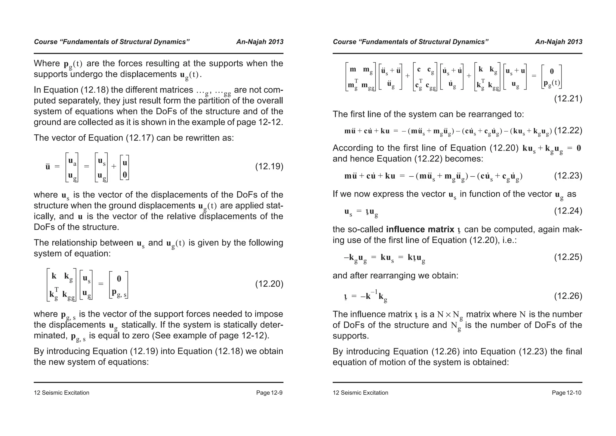
![Course “Fundamentals of Structural Dynamics” An-Najah 2013
12 Seismic Excitation Page12-11
(12.27)
Analogously, with the second line of Equation (12.21), an equa-
tion for the computation of the forces at the supports can
be setup and solved.
Remarks
In Equation (12.27), the masses associated with the support are
often equal to zero, i.e. . If this is the case, Equation
(12.27) simplifies to:
(12.28)
And considering that in most cases the damping forces on the
LHS of the equation are small (and they are zero if no damping
is present) compared to the inertia forces (see [Cho11]), Equa-
tion (12.28) can be further simplified to:
(12.29)
In the case that the movement of the supports is the same at all
supports, becomes:
(12.30)
and with Equation (12.29) becomes
(12.31)
which is the same as Equation (12.10).
mu·· cu· ku+ + mι mg+( )u··
g– cι cg+( )u·
g–=
pg t( )
mg 0=
mu·· cu· ku+ + mιu··
g– cι cg+( )u·
g–=
mu·· cu· ku+ + mιu··
g–=
ug
ug 1ug=
ι ι1=
mu·· cu· ku+ + mιu··
g–=
Course “Fundamentals of Structural Dynamics” An-Najah 2013
12 Seismic Excitation Page12-12
Example: 2-DoF system
The following 2-DoF system is subjected to multiple support
ground motion. Two different ground motions are applied to the
degrees of freedom and . Sought is the equation of motion
of the system:
The stiffness matrix of the system is assembled by means of the
Direct Stiffness Method and the following degrees of freedom
are considered:
: displacements of the structure (12.32)
: displacements of the supports (excited, massless)
(12.33)
: displacements of the supports (not excited, massless)
(12.34)
The stiffness matrix of the system is:
u1 u5
u
u3
u4
=
ug
u1
u5
=
u0
u2
u6
=
K](https://image.slidesharecdn.com/fundamentalsofstructuraldynamics-200730194708/75/Fundamentals-of-structural-dynamics-157-2048.jpg)
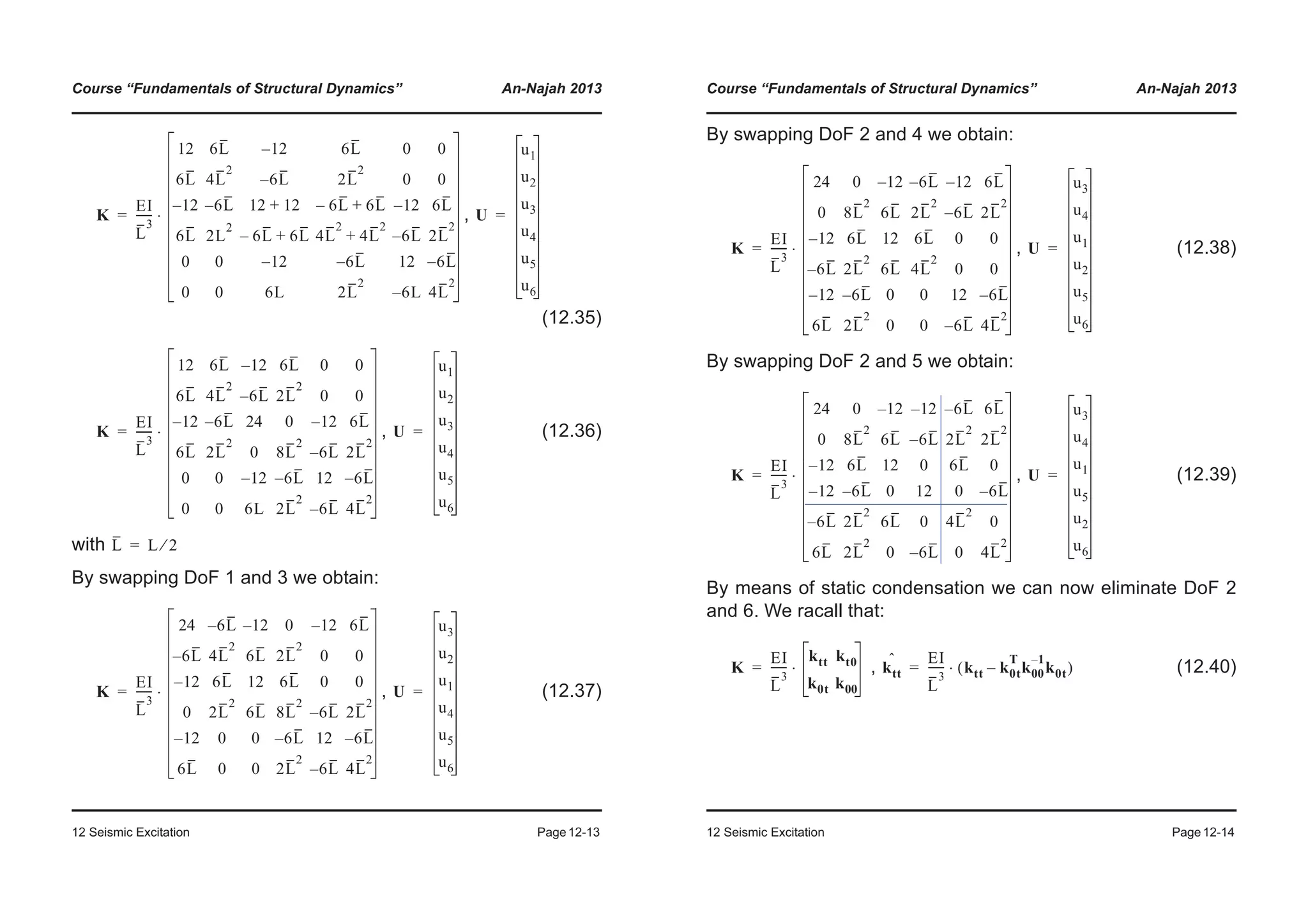
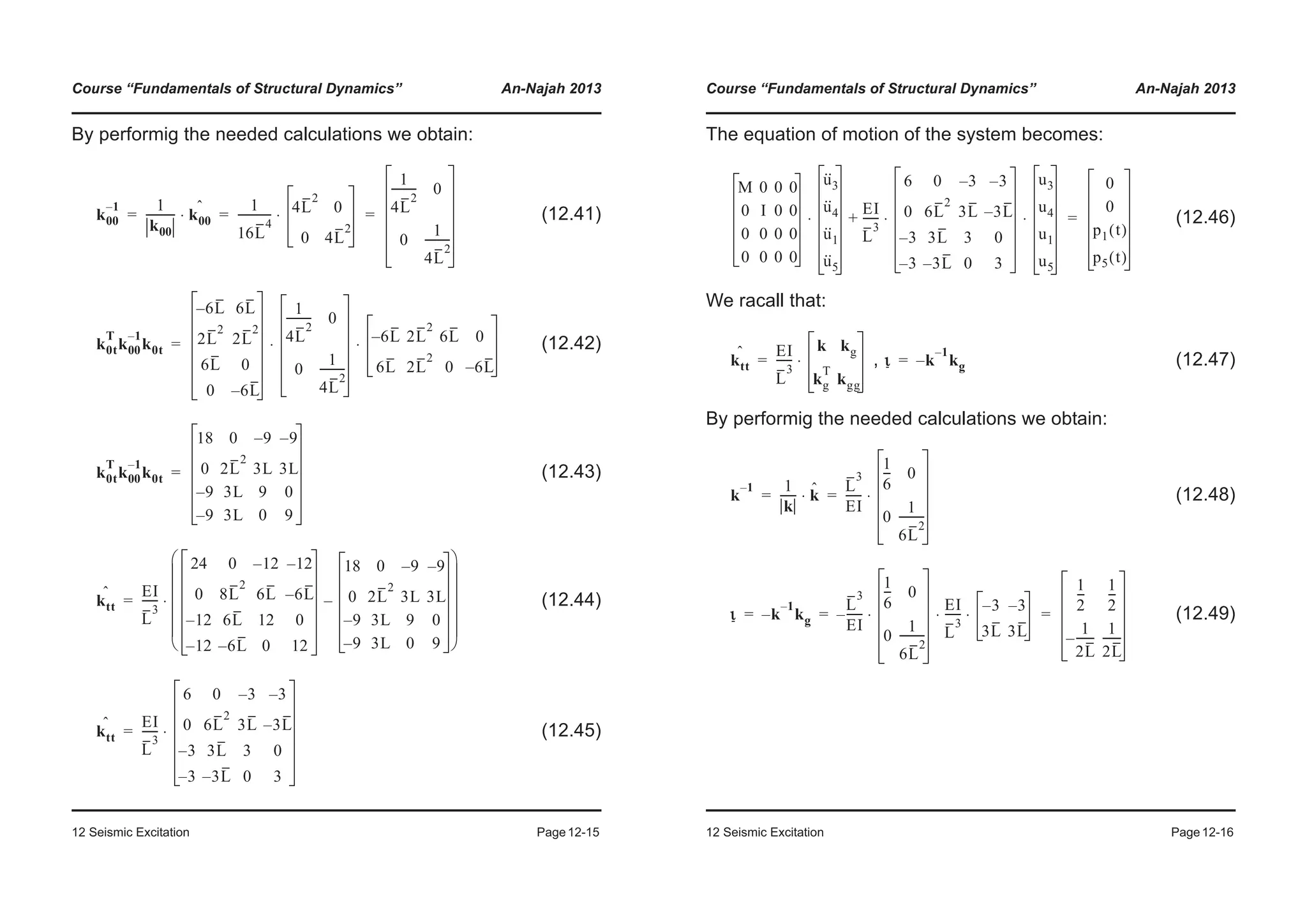
![Course “Fundamentals of Structural Dynamics” An-Najah 2013
12 Seismic Excitation Page12-17
The vector of the effective forces becomes:
(12.50)
And the equation of motion of the system finally becomes:
(12.51)
The following drawings show the interpretation of the elements
of the influence matrix :
Remarks:
• See Section 9.7 of [Cho11] for an example with a statically in-
determinated system.
• In Finite Element analysis, when applying multiple support ex-
citation, support displacements instead of support acceleration
are often used. For more details see [Bat96].
if then:
and
if then:
and
peff t( ) mι mg+( )u··
g t( )–
M
2
-----
M
2
-----
I
2L
-------–
I
2L
-------
–
u··
g1
u··
g5
⋅= =
M 0
0 I
u··
3
u··
4
EI
L
3
------
6 0
0 6L
2
u3
u4
⋅ ⋅+⋅
M
2
-----
M
2
-----
I
2L
-------–
I
2L
-------
–
u··
g1
u··
g5
⋅=
ι
ug1 1=
u3
1
2
---= u4
1
2L
-------–=
ug5 1=
u3
1
2
---= u4
1
2L
-------=
Course “Fundamentals of Structural Dynamics” An-Najah 2013
12 Seismic Excitation Page12-18
12.2 Time-history of the response of elastic systems
As discussed in the previous sections, the equation of motion of
a MDoF system under base excitation is:
(12.52)
Where:
: Mass matrix (symmetric and positive-definite, or diag-
onal if only lumped masses are present)
: Stiffness matrix (symmetric and positive-definite)
: Damping matrix (Classical damping: is typically a
linear combination of and )
: Ground acceleration
: Influence vector of order . In the simplest case of a
planar system under translational ground motion .
If the damping of the MDoF system is classical, Equation (12.52)
can be written in the form of decoupled modal equations,
where is the number of modes of the system. The modal
equations are of the following form:
(12.53)
or:
(12.54)
The dynamic response of the MDoF system can be written as:
Mu·· Cu· Ku+ + Mιu··
g t( )–=
M
K
C C
M K
u··
g t( )
ι N
ι 1=
N
N
mn
*q··
n cn
*q·
n kn
*qn+ + φn
T
Mιu··
g–=
q··
n 2ζn
*ωnq·
n ωn
2
qn+ +
φn
T
Mι
φn
T
Mφn
------------------u··
g–=](https://image.slidesharecdn.com/fundamentalsofstructuraldynamics-200730194708/75/Fundamentals-of-structural-dynamics-160-2048.jpg)
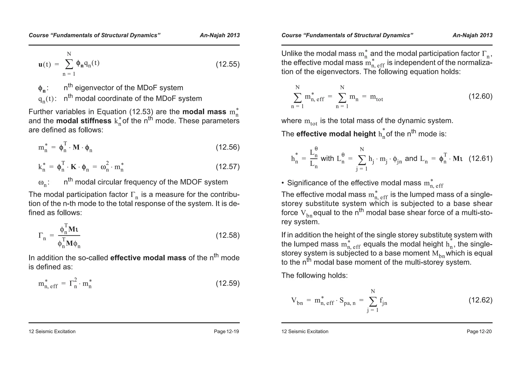
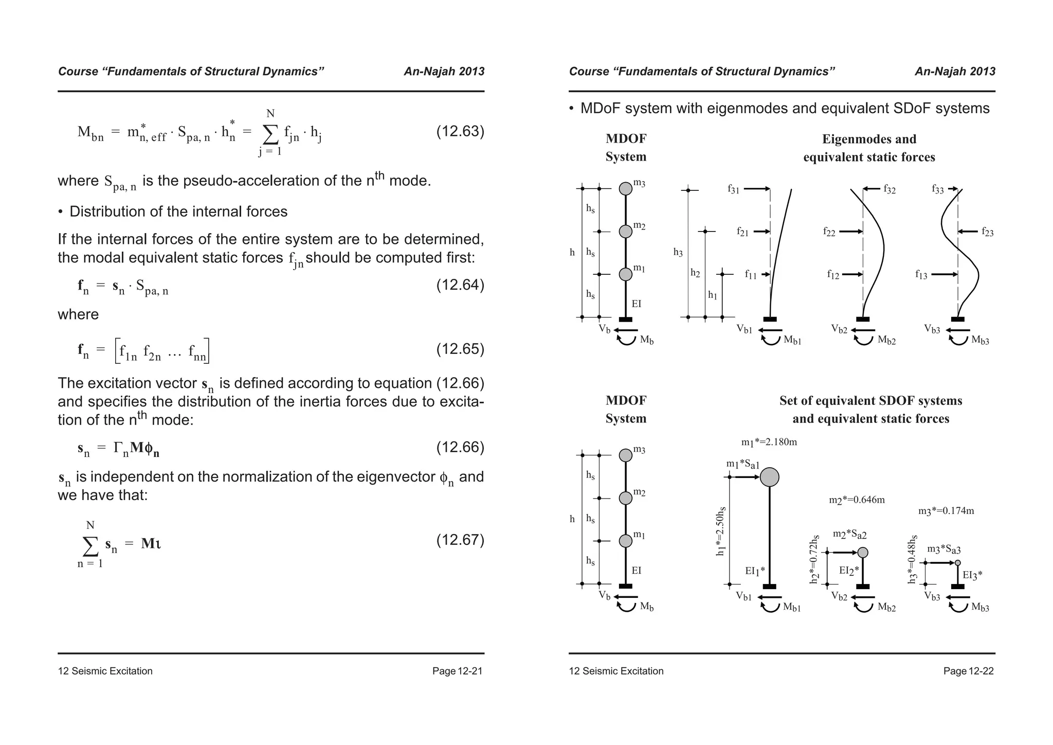
![Course “Fundamentals of Structural Dynamics” An-Najah 2013
12 Seismic Excitation Page12-25
with
(12.73)
This method based on random vibration theory gives exact re-
sults if the excitation is represented by a white noise. If the fre-
quencies of the modes are well spaced apart, the result converge
to those of the SRSS rule. More detailed information on this and
other combination rules can be found in [Cho11] Chapter 13.7.
• Internal forces
The aforementioned combination rules cannot only be applied
on displacements but also on internal forces.
The maximum modal internal forces can be determined from
equivalent static forces
, (12.74)
which, as a first option, are computed from the equivalent static
displacements. Alternatively, the equivalent static forces can be
determined from the inertia forces:
(12.75)
with being the excitation vector which represents the distribu-
tion of the inertia forces of the nth
mode (see Equation 12.67).
Attention:
It is wrong to compute the maximum internal forces from the
maximum displacement of the total response .
ρjk
8 ζiζk ζi rζk+( )r3 2⁄
1 r2–( )2 4ζiζkr 1 r2+( ) 4 ζi
2 ζk
2+( )r2+ +
----------------------------------------------------------------------------------------------------= r
ωk
ωj
------=
Fn max, K un max,⋅=
Fn max, sn Spa ωn ζn
*( , )⋅ ΓnMφn Spa ωn ζn
*( , )⋅= =
sn
umax
Course “Fundamentals of Structural Dynamics” An-Najah 2013
12 Seismic Excitation Page12-26
• Number of modes to be considered.
All modes which contribute to the dynamic response of the sys-
tem should be considered. In practical applications, however,
only those modes are considered which contribution to the total
response is above a certain threshold. It should be noted that in
order to achieve the same accuracy for different response meas-
ures (e.g. displacements, shear forces, bending moments, etc.)
different numbers of modes might need to be considered in the
computation.
For a regular building the top displacement can be estimated
fairly well on the basis of the fundamental mode only. To esti-
mate the internal forces, however, higher modes need to be con-
sidered too.
According to Eurocode 8 “Design of Structures for Earthquake
Resistance” [CEN04] all modes should be considered (starting
from the lowest) until the sum of the effective modal masses
of all considered modes corresponds to at least 90% of
the total mass . As an alternative, Eurocode 8 allows the de-
signer to show that all modes with were consid-
ered in the computation.
mn eff,
mtot
mn eff,
* 0.05mtot>](https://image.slidesharecdn.com/fundamentalsofstructuraldynamics-200730194708/75/Fundamentals-of-structural-dynamics-164-2048.jpg)
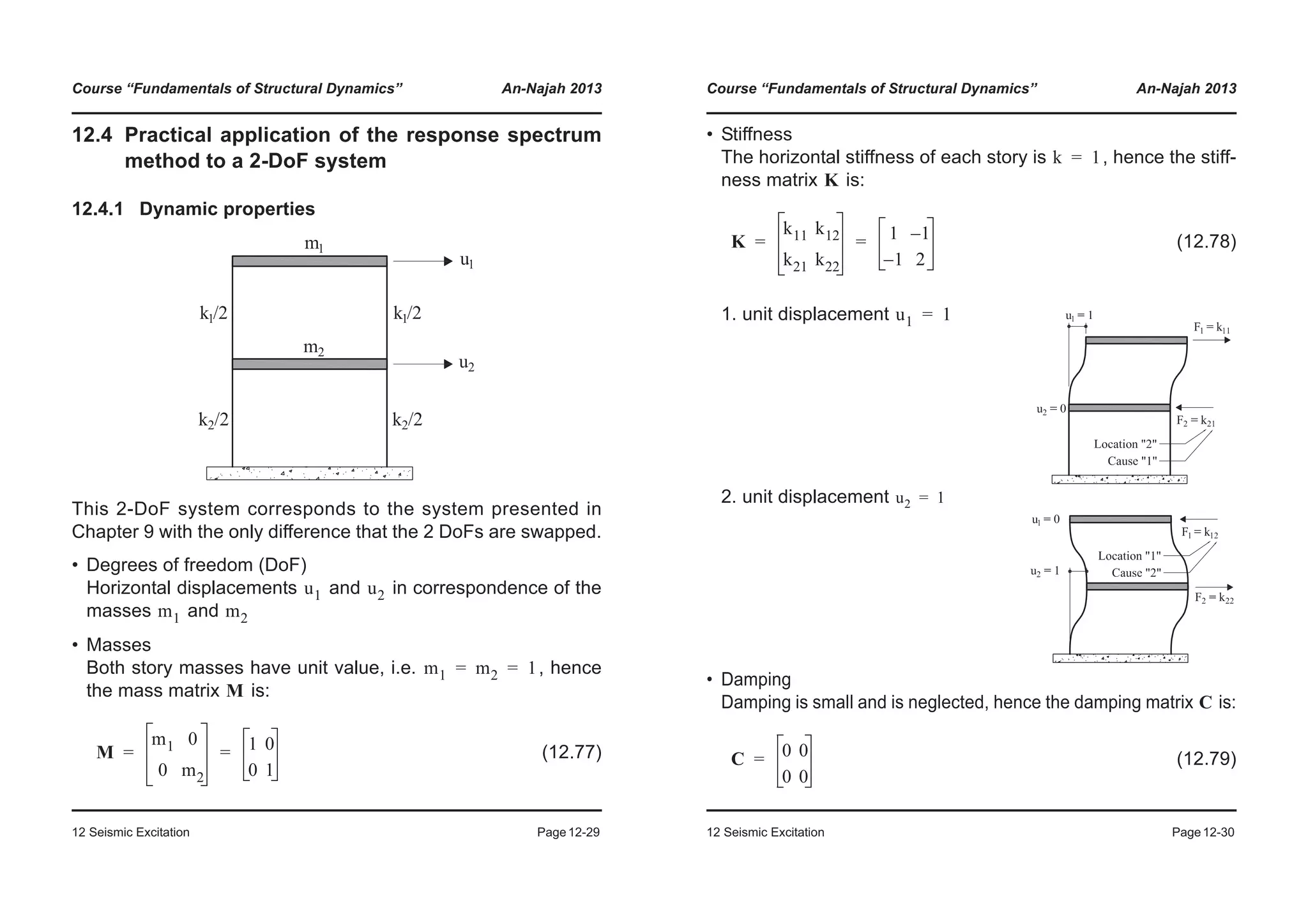
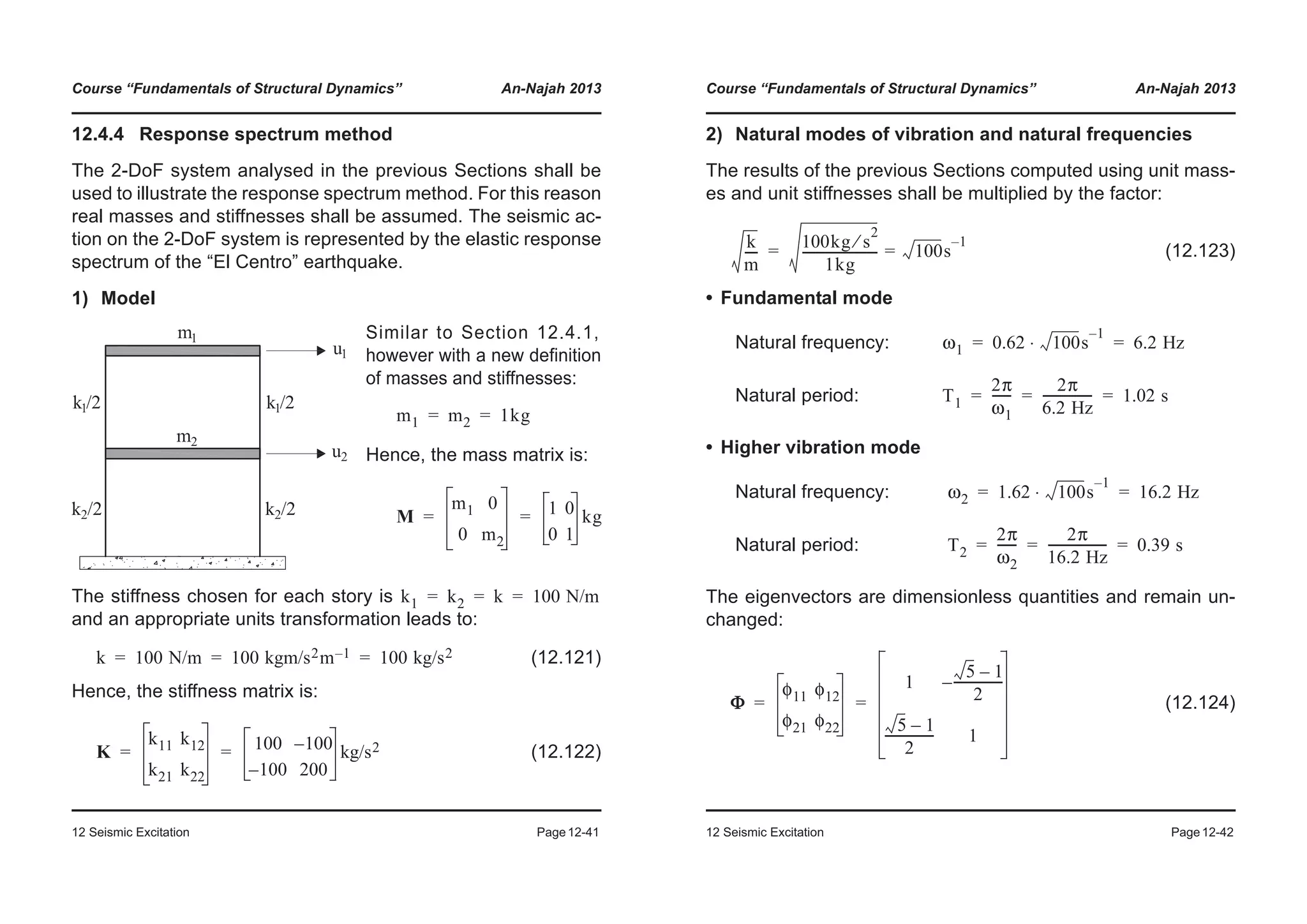
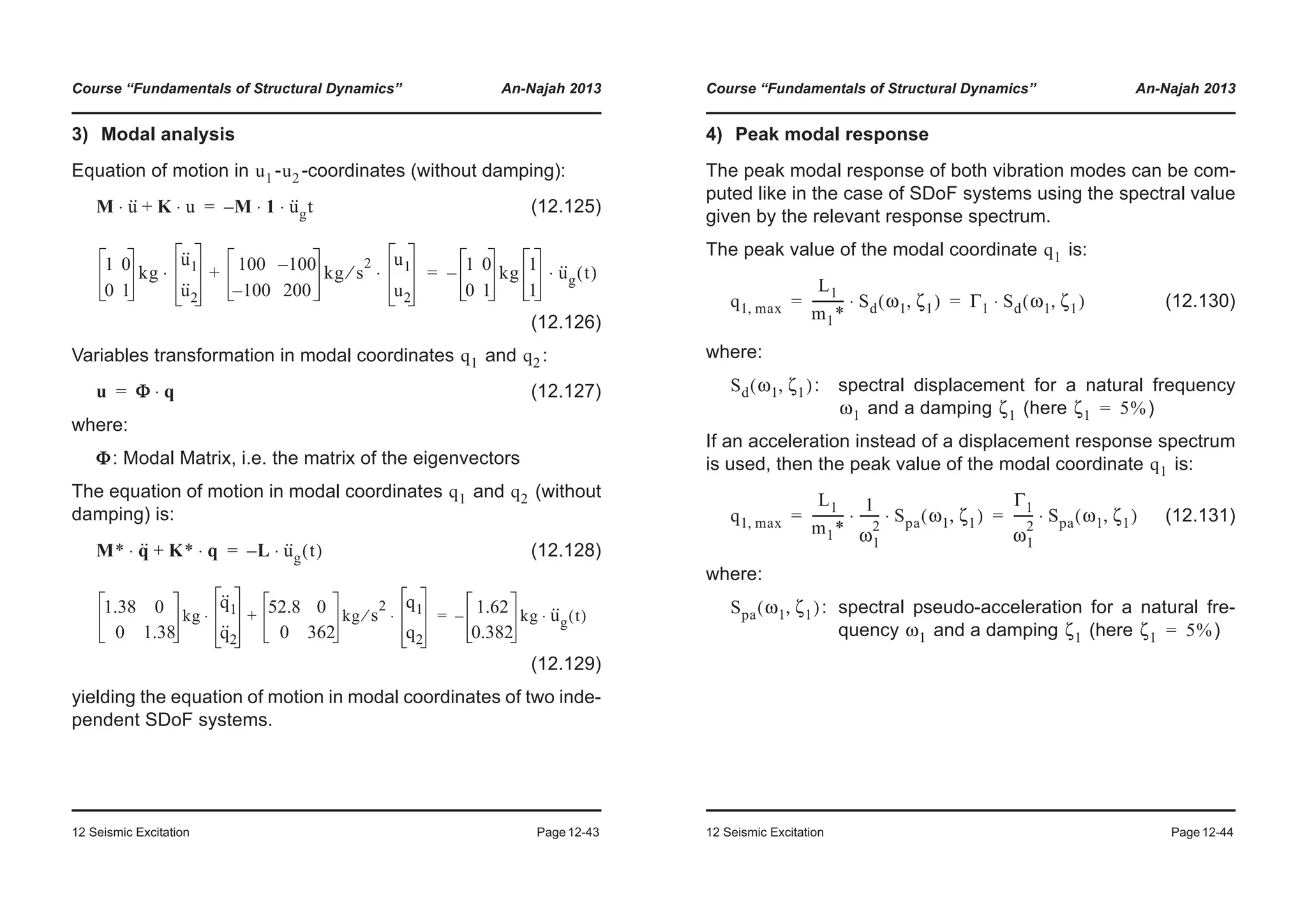
![Course “Fundamentals of Structural Dynamics” An-Najah 2013
12 Seismic Excitation Page12-45
The spectral values given by the elastic acceleration response
spectrum of the “El Centro” earthquake for the periods and
are:
and (12.132)
(12.133)
(12.134)
(12.135)
T1
T2
Spa1 4.25 m/s2=
Spa2 7.34 m/s2=
0.01 0.10 1.00 10.0
Period [s]
0
5
10
Pseudoacceleration[m/s]2
Spa2 = 7.34 m/s2
Spa1 = 4.25 m/s2
T2 = 0.39 s T1 = 1.02 s
ζ = 5%
q1 max,
1.62kg
1.38kg
-----------------
1
6.2Hz( )2
---------------------- 4.25 m/s2⋅ ⋅ 0.130m= =
q2 max,
0.38kg
1.38kg
-----------------
1
16.2Hz( )2
------------------------- 7.34 m/s2⋅ ⋅ 0.008m= =
Course “Fundamentals of Structural Dynamics” An-Najah 2013
12 Seismic Excitation Page12-46
5) Inverse transformation
The peak deformations and internal forces belonging to each mode of vibra-
tion in the original reference system are obtained by multiplying the relevant
eigenvector with the corresponding peak value of the modal coordinate.
• Fundamental mode
(12.136)
(12.137)
Alternatively (allow an approximate consideration of nonlinearities):
(12.138)
(12.139)
umax
1( )
q1 max, φ1⋅ 0.130m 1
0.62
⋅ 130
81
mm= = =
fmax
1( )
K umax
1( )
⋅ 100 100–
100 200
0.130
0.081
⋅ 13.0 8.1–
13.0– 16.2+
4.9
3.2
N= = = =
s1 Γ1Mφ1 1.17 1 0
0 1
1
0.62
⋅ ⋅ 1.17
0.725
= = =
fmax
1( )
s1 Spa1⋅ 4.25 1.17
0.725
4.9
3.2
N= = =](https://image.slidesharecdn.com/fundamentalsofstructuraldynamics-200730194708/75/Fundamentals-of-structural-dynamics-174-2048.jpg)
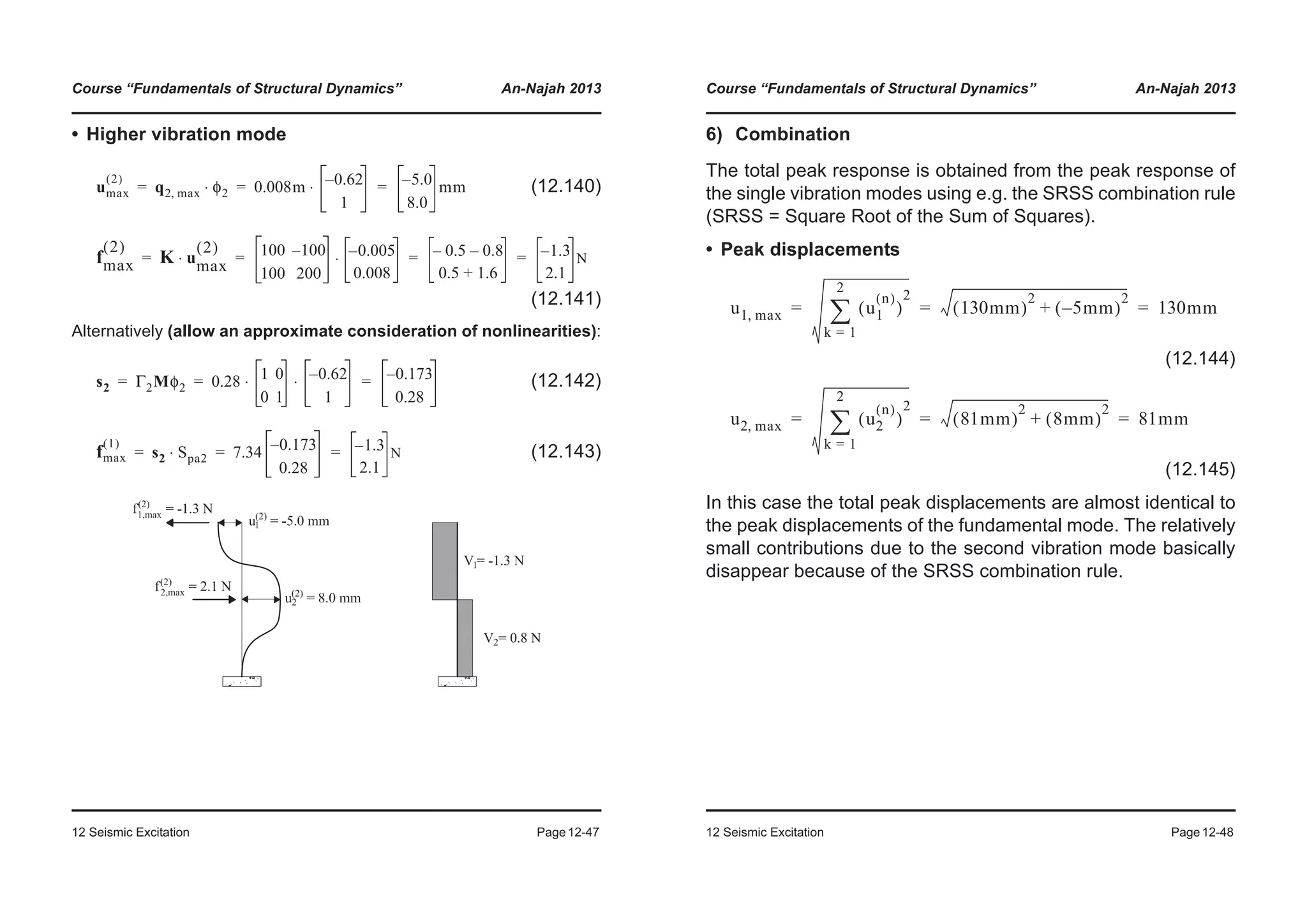
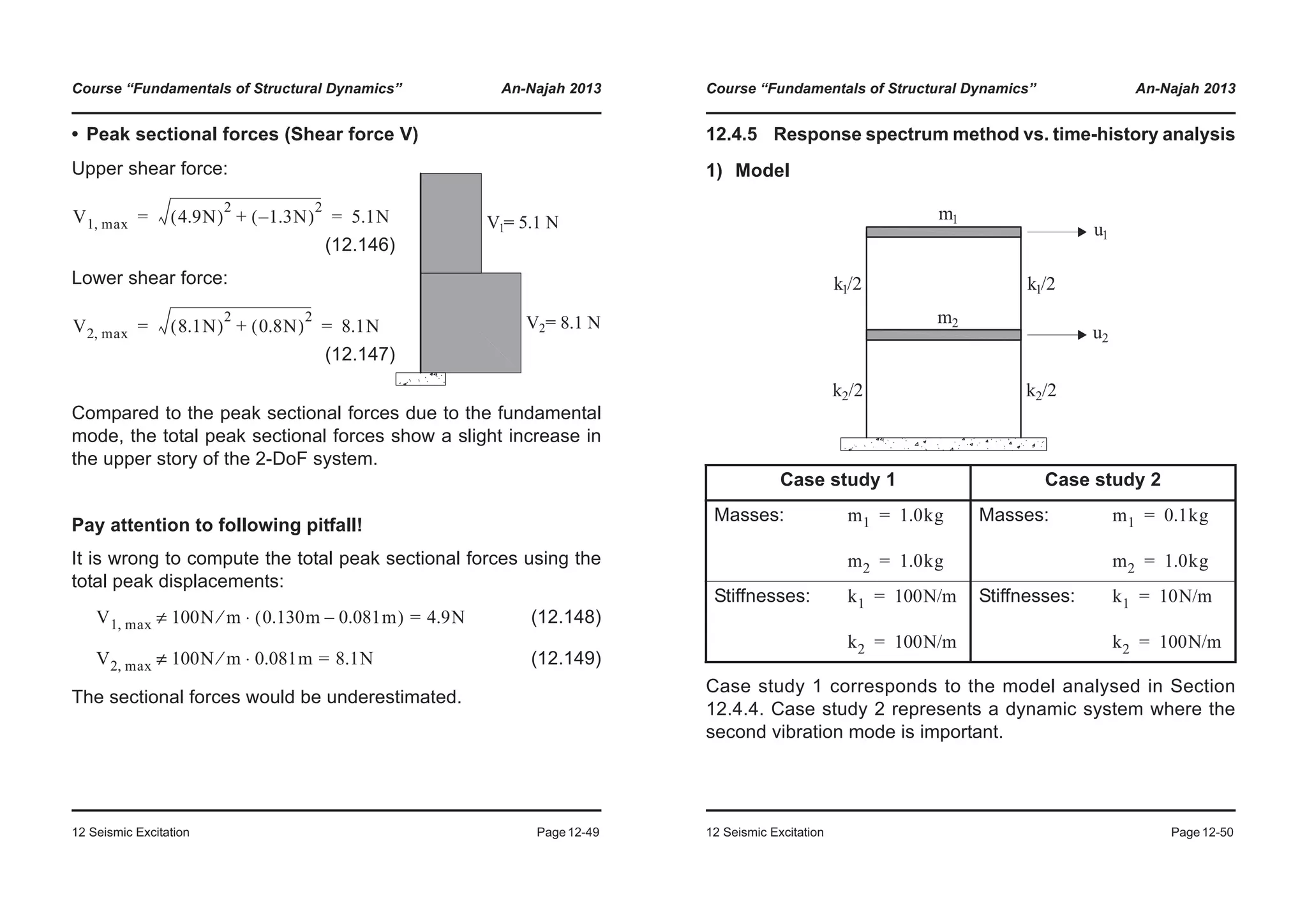
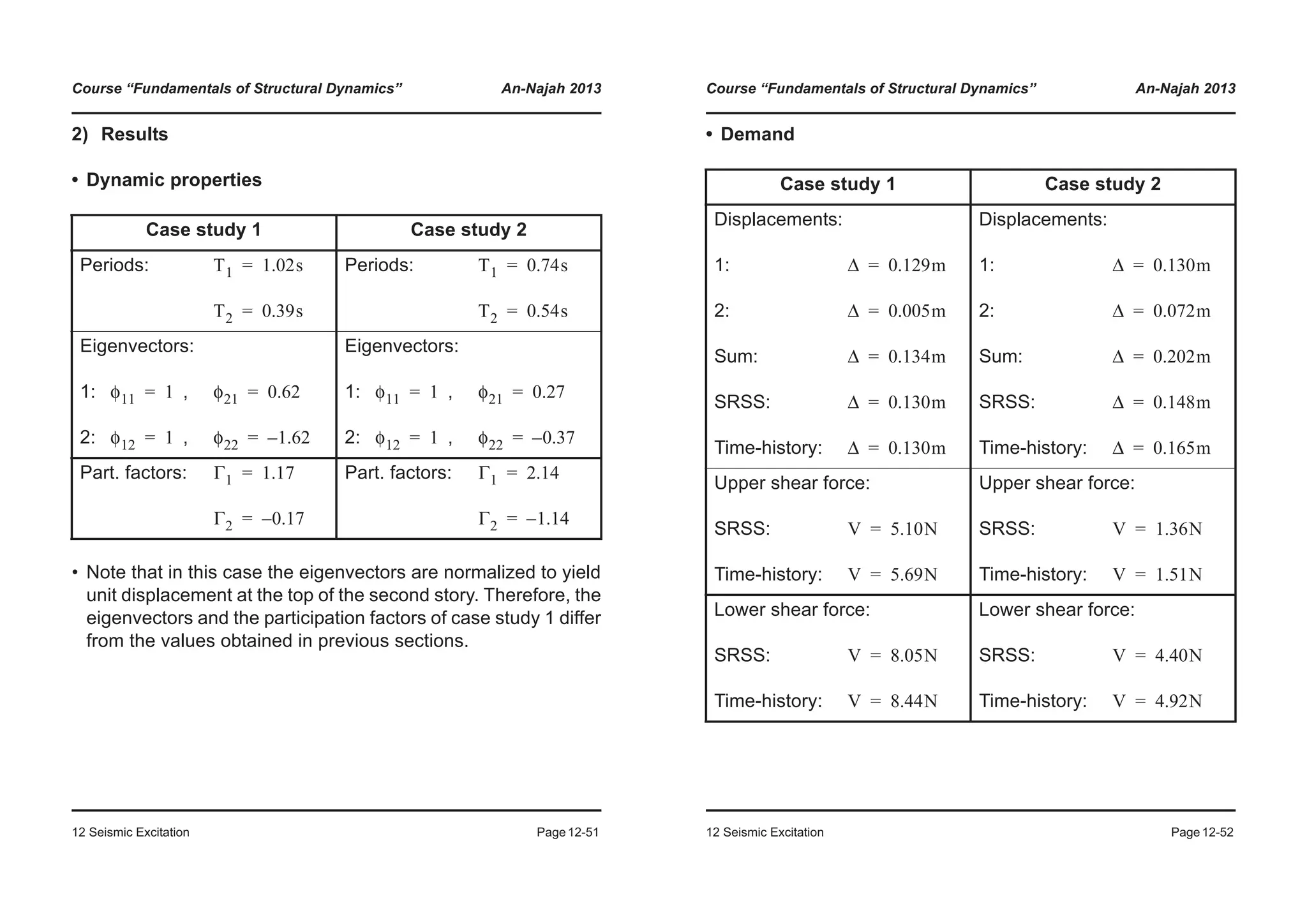
![Course “Fundamentals of Structural Dynamics” An-Najah 2013
12 Seismic Excitation Page12-53
• Time-histories: Case study 1
0 5 10 15 20
−20
−10
0
10
20
Displacement[cm]
0 5 10 15 20
−20
−10
0
10
20
Displacement[cm]
0 5 10 15 20
Time [s]
−20
−10
0
10
20
Displacement[cm]
First mode
Second mode
Sum
Course “Fundamentals of Structural Dynamics” An-Najah 2013
12 Seismic Excitation Page12-54
• Time-histories: Case study 2
0 5 10 15 20
−20
−10
0
10
20
Displacement[cm]
0 5 10 15 20
−20
−10
0
10
20
Displacement[cm]
0 5 10 15 20
Time [s]
−20
−10
0
10
20
Displacement[cm]
First mode
Second mode
Sum
Peak values don’t occur at the same time!](https://image.slidesharecdn.com/fundamentalsofstructuraldynamics-200730194708/75/Fundamentals-of-structural-dynamics-178-2048.jpg)
![Course “Fundamentals of Structural Dynamics” An-Najah 2013
12 Seismic Excitation Page12-55
• Time-histories: Summary
0 5 10 15 20
−20
−10
0
10
20
Displacement[cm]
0 5 10 15 20
Time [s]
−20
−10
0
10
20
Displacement[cm]
First mode
Second mode
Sum
First mode
Second mode
Sum
Case study 1
Case study 2
Course “Fundamentals of Structural Dynamics” An-Najah 2013
12 Seismic Excitation Page12-56
Blank page](https://image.slidesharecdn.com/fundamentalsofstructuraldynamics-200730194708/75/Fundamentals-of-structural-dynamics-179-2048.jpg)
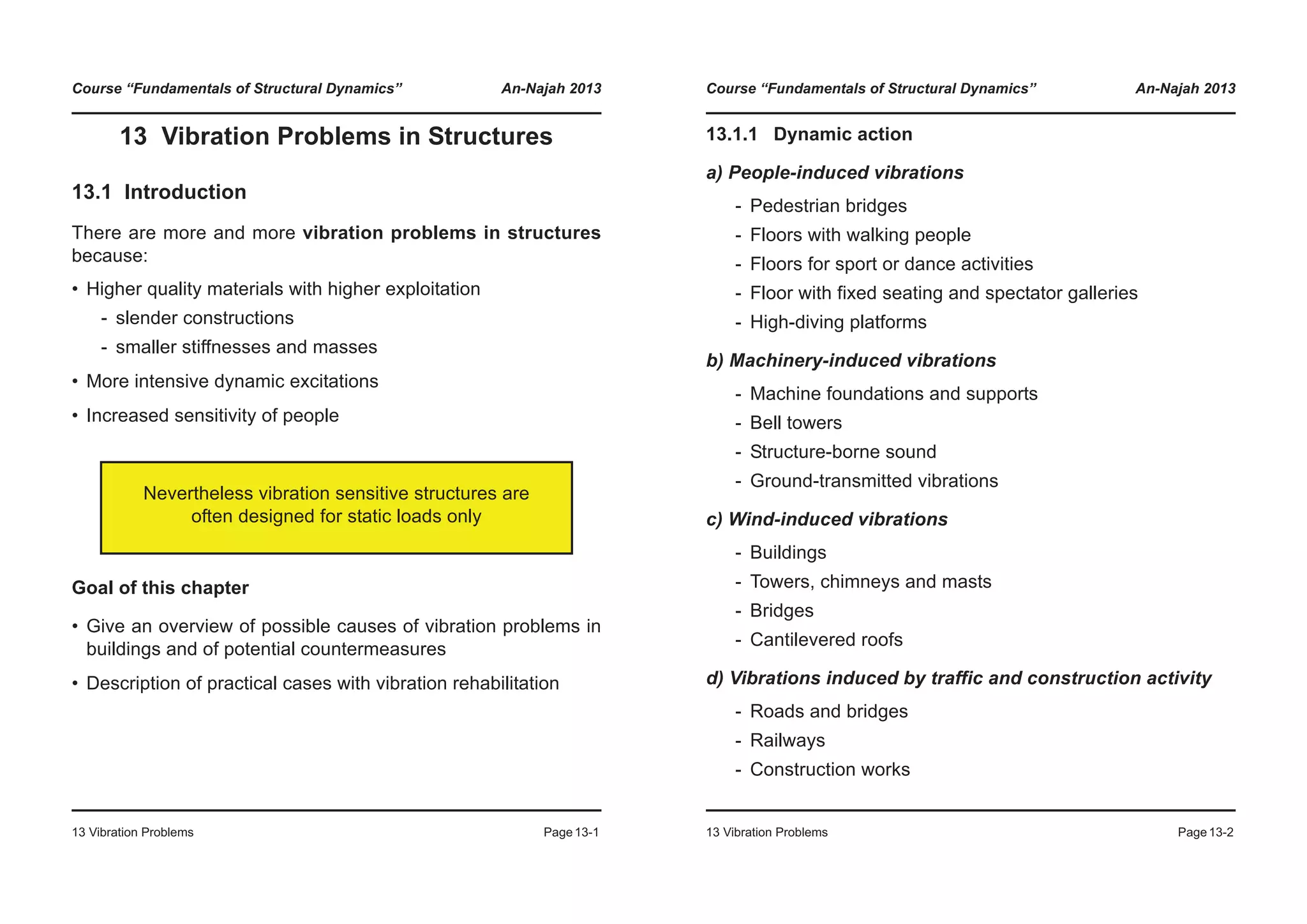
![Course “Fundamentals of Structural Dynamics” An-Najah 2013
13 Vibration Problems Page13-3
13.1.2 References
[Bac+97] Bachmann et al.:”Vibration Problems in Structures”.
ISBN 3-7643-5148-9. Birkhäuser Verlag, Basel 1997.
[BB88] Baumann K., Bachmann H.: “Durch Menschen verursachte
dynamische Lasten und deren Auswirkungen auf Balkentrag-
werke”. IBK Bericht Nr. 7501-3, 1988.
[BW95] Bachmann H., Weber B.: “Tuned Vibration Absorbers for
Damping of Lively Structures”. Structural Engineering Inter-
national, No. 1, 1995.
[SIA06] SIA: “Wind – Kommentar zum Kapitel 6 der Normen SIA 261
und 261/1 (2003) Einwirkungen auf Tragwerke”. SIA Doku-
mentation D0188. Zürich 2006.
[SIA03] SIA: “Aktuelle Probleme der Brückendynamik”. SIA Doku-
mentation D0198. Zürich 2003.
[SIA96] SIA: “Dynamische Probleme bei Brücken- und Hochbauten”.
SIA Dokumentation D0138. Zürich 1996.
[VB87] Vogt R., Bachmann H.: “Dynamische Kräfte beim Klatschen,
Fussstampfen und Wippen”. IBK Bericht Nr. 7501-4, 1987.
Course “Fundamentals of Structural Dynamics” An-Najah 2013
13 Vibration Problems Page13-4
13.2 Vibration limitation
13.2.1 Verification strategies
• Frequency tuning
- High tuning (subcritical excitation)
- Low tuning (supercritical excitation)
• Amplitude limitation
3
4
5
6
7
8
9
10
rasmissibilityTR
0.00
0.10
0.01
ζ = 0.05
0
1
2
3
0 0.5 1 1.5 2 2.5 3 3.5 4
Tr
ω/ωn
0.20
0.50
0.70 2](https://image.slidesharecdn.com/fundamentalsofstructuraldynamics-200730194708/75/Fundamentals-of-structural-dynamics-181-2048.jpg)
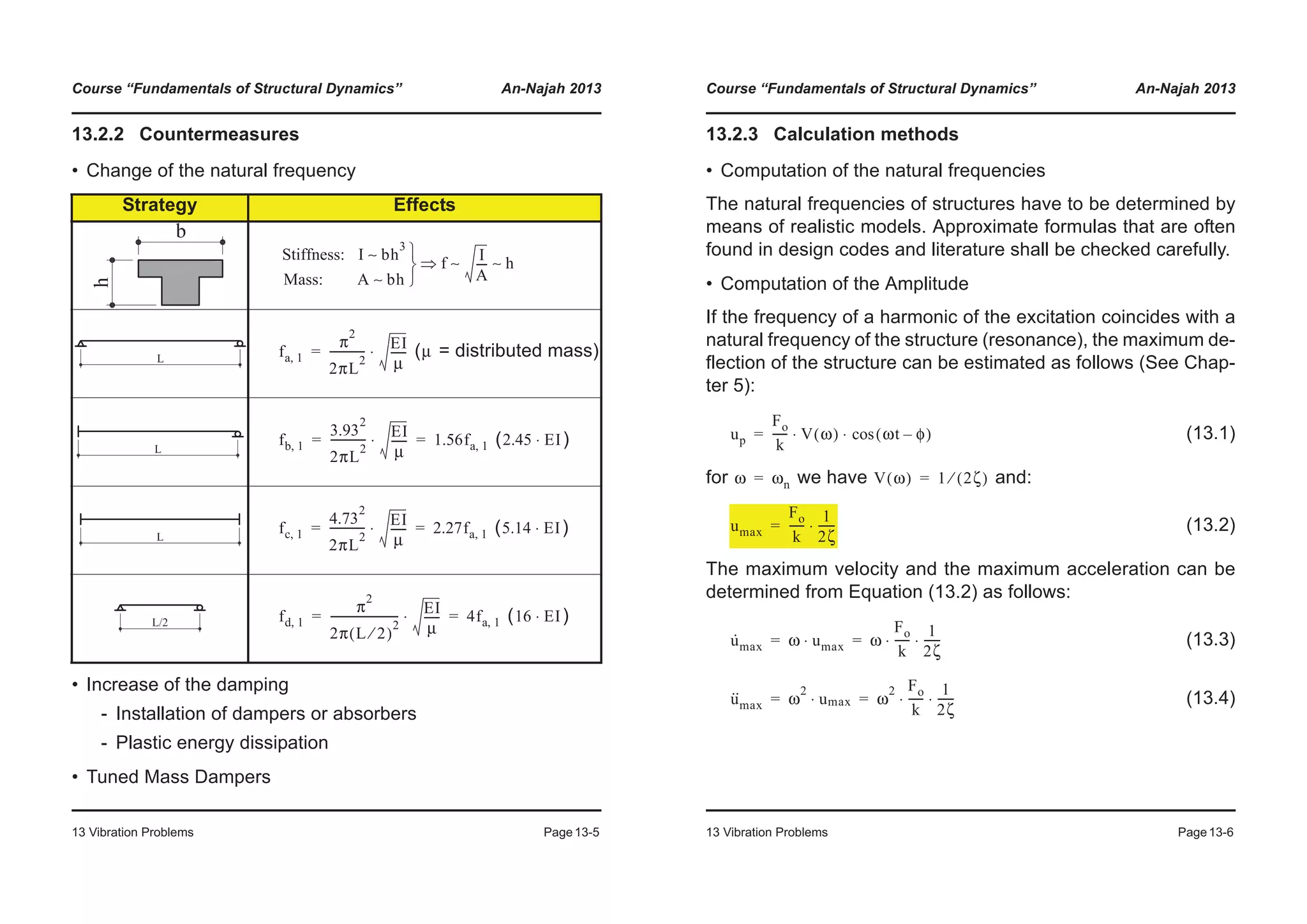
![Course “Fundamentals of Structural Dynamics” An-Najah 2013
13 Vibration Problems Page13-7
The amplitude of the nth harmonic component of a force gener-
ated by people excitation is proportional to the mass of the per-
son ( , see Equation (13.8)).
(13.5)
(13.6)
• Remarks
- A soft structure is more prone to vibration than a rigid one.
See Equations (13.2) to (13.4).
- The acceleration amplitude is directly proportional on the
ratio of the mass of the people to the building mass.
Fo G αn⋅ g M αn⋅ ⋅= =
u··
max ω
2 g M αn⋅ ⋅
k
-----------------------
1
2ζ
------⋅ ⋅
k
m
----
g M αn⋅ ⋅
k
-----------------------
1
2ζ
------⋅ ⋅
M
m
-----
g αn⋅
2ζ
-------------⋅= = =
u··
max
M
m
-----
g αn⋅
2ζ
-------------⋅=
Course “Fundamentals of Structural Dynamics” An-Najah 2013
13 Vibration Problems Page13-8
13.3 People induced vibrations
13.3.1 Excitation forces
In Chapter 6 “Forced Vibrations” it has been already mentioned
that excitation due to people, like e.g. walking, running, jumping,
and so on, can be represented as Fourier-series:
(13.7)
Equation (13.7) can also be represented in a form according to
Equation (13.8):
(13.8)
Where:
- = Weight of the person
- = Fourier coefficient for the nth harmonic
- = Amplitude of the nth
harmonic of the excitation force
- = Step frequency of the excitation force
- = Phase shift of the nth harmonic ( )
- = Number of the nth
harmonic
- = Number of considered harmonics
F t( ) a0 an nω0t( )cos bn nω0t( )sin+[ ]
n 1=
∞
¦+=
F t( ) G G αn n 2πf0 t φn–⋅ ⋅( )sin⋅ ⋅
n 1=
N
¦+=
G
αn
G αn⋅
f0
φn φ1 0=
n
N](https://image.slidesharecdn.com/fundamentalsofstructuraldynamics-200730194708/75/Fundamentals-of-structural-dynamics-183-2048.jpg)
![Course “Fundamentals of Structural Dynamics” An-Najah 2013
13 Vibration Problems Page13-9
The steady-state response of a SDoF system under periodic ex-
citation can be computed in analogy to Chapter 6 as:
(13.9)
Where
(Static displacement) (13.10)
(13.11)
, (13.12)
• Measurement of forces (Example)
u t( ) u0 t( ) un t( )
n 1=
N
¦+=
u0 t( )
G
k
----=
un t( )
G αn⋅
k
---------------
1 βn
2
–( ) nω0t φn–( )sin 2ζβn nω0t φn–( )cos–
1 βn
2
–( )
2
2ζβn( )
2
+
----------------------------------------------------------------------------------------------------------------⋅=
ω0 2πf0= βn
nω0
ωn
---------=
Course “Fundamentals of Structural Dynamics” An-Najah 2013
13 Vibration Problems Page13-10
• Jumping (left) and walking (right), see [BB88]
• Clapping, foot stomping and rocking, see [VB87]](https://image.slidesharecdn.com/fundamentalsofstructuraldynamics-200730194708/75/Fundamentals-of-structural-dynamics-184-2048.jpg)
![Course “Fundamentals of Structural Dynamics” An-Najah 2013
13 Vibration Problems Page13-11
• Walking (see [Bac+97] Figure G.1)
• Clapping (see [Bac+97] Figure G.3)
Course “Fundamentals of Structural Dynamics” An-Najah 2013
13 Vibration Problems Page13-12
• Jumping (see [Bac+97] Figure G.2)
• Jumping: Fourier amplitude spectrum (see [Bac+97] Figure G.2)](https://image.slidesharecdn.com/fundamentalsofstructuraldynamics-200730194708/75/Fundamentals-of-structural-dynamics-185-2048.jpg)
![Course “Fundamentals of Structural Dynamics” An-Najah 2013
13 Vibration Problems Page13-13
Characterisationofhumanactivitiesaccordingto[Bac+97]TableG.1
Course “Fundamentals of Structural Dynamics” An-Najah 2013
13 Vibration Problems Page13-14
Fourier-coefficientsforhumanactivitiesaccordingto[Bac+97]TableG.2](https://image.slidesharecdn.com/fundamentalsofstructuraldynamics-200730194708/75/Fundamentals-of-structural-dynamics-186-2048.jpg)
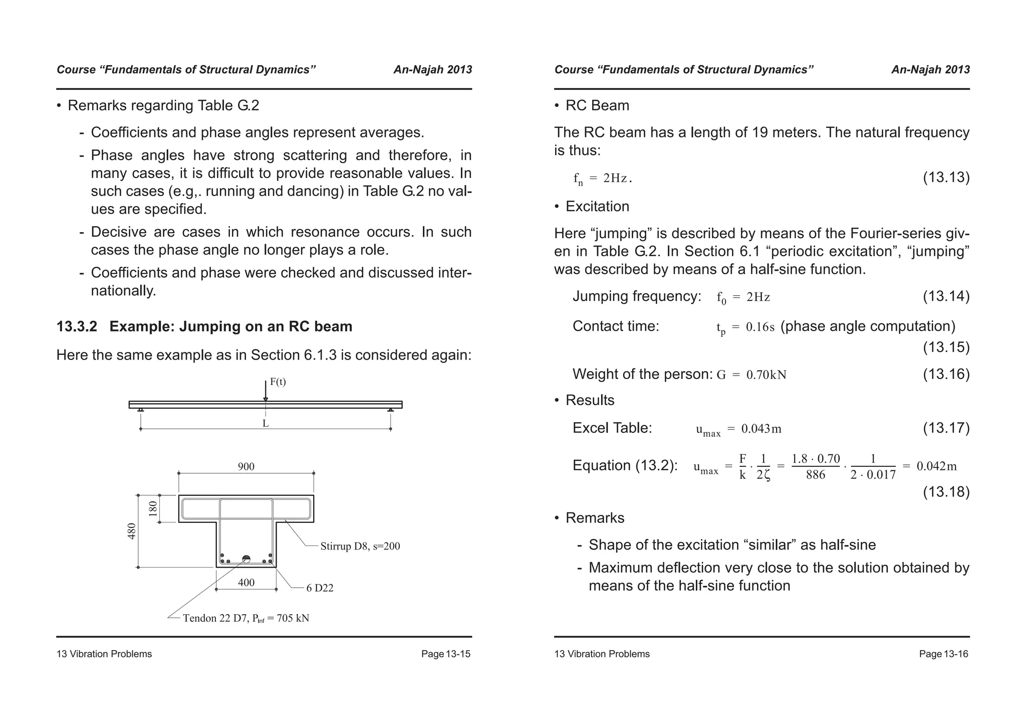
![Course “Fundamentals of Structural Dynamics” An-Najah 2013
13 Vibration Problems Page13-17
• Excitation
• Response
0 0
0.5
1.0
1.5
2.0
2.5
3.0
3.5
ForceF(t)[kN]
Static component (n=0)
First harmonics (n=1)
Second harmonics (n=2)
Third harmonics (n=3)
Total (3 harmonics)
-1.5
-1.0
-0.5
0.0
0 0.1 0.2 0.3 0.4 0.5 0.6 0.7 0.8 0.9 1
Time (s)
0 0200
-0.0100
0.0000
0.0100
0.0200
0.0300
0.0400
0.0500
Displacement[m]
Static component (n=0)
First harmonics (n=1)
Second harmonics (n=2)
Third harmonics (n=3)
Total (3 harmonics)
-0.0500
-0.0400
-0.0300
-0.0200
0 0.1 0.2 0.3 0.4 0.5 0.6 0.7 0.8 0.9 1
D
Time (s)
Course “Fundamentals of Structural Dynamics” An-Najah 2013
13 Vibration Problems Page13-18
13.3.3 Footbridges
• Frequency tuning
- Vertical: Avoid natural frequencies between 1.6 and
2.4Hz. In the case of structures with low damping (Steel),
avoid also natural frequencies from 3.5 to 4.5Hz.
- Horizontal transverse: Avoid natural frequencies be-
tween 0.7 and 1.3Hz (absolutely safe: fht,1 > 3.4Hz).
- Horizontal longitudinal: Avoid natural frequencies be-
tween 1.6 and 2.4Hz.
• Amplitude limitation
- Calculation of the acceleration maximum amplitude.
(13.19)
• Special features of the amplitude limitation
- When walking or running, the effectiveness of people is lim-
ited, because the forces are not always applied at midspan;
System
Equivalent
SDoF system
amax ca. 0.5m s
2
⁄< 5% g=](https://image.slidesharecdn.com/fundamentalsofstructuraldynamics-200730194708/75/Fundamentals-of-structural-dynamics-188-2048.jpg)
![Course “Fundamentals of Structural Dynamics” An-Najah 2013
13 Vibration Problems Page13-19
- People need a finite number of steps in order to cross the
bridge (This limited excitation time may be too short to
reach the maximum amplitude)
- Not all people walk in the step (Exception: Lateral vibra-
tions Synchronisation effect)
To take into account the specificities of the amplitude limitation,
sophisticated methods are available. From [Bac+97] the follow-
ing one is adopted:
(13.20)
Where:
- : Static deflection at half the span
- : Fourier coefficient
- : dynamic amplification factor
0.4
0.6
0.8
1
abs(uj)/umax
ζ = 0.01
0.02
0.050.1
0.2
0
0.2
0 5 10 15 20 25 30 35 40 45 50
Cycle
→
amax 4π
2
f
2
y α Φ⋅ ⋅ ⋅ ⋅= m s
2
⁄[ ]
y
α
Φ
Course “Fundamentals of Structural Dynamics” An-Najah 2013
13 Vibration Problems Page13-20
The acceleration given in Equation (13.20) is the accelera-
tion generated by one person crossing the footbridge. If people
are on the bridge at the same time, the maximum acceleration is
typically less than because not all people walk in step
across the bridge.
.
The square root of the number of people is often
chosen as the multiplication factor, i.e.
amax
n
n amax⋅
n amax⋅](https://image.slidesharecdn.com/fundamentalsofstructuraldynamics-200730194708/75/Fundamentals-of-structural-dynamics-189-2048.jpg)
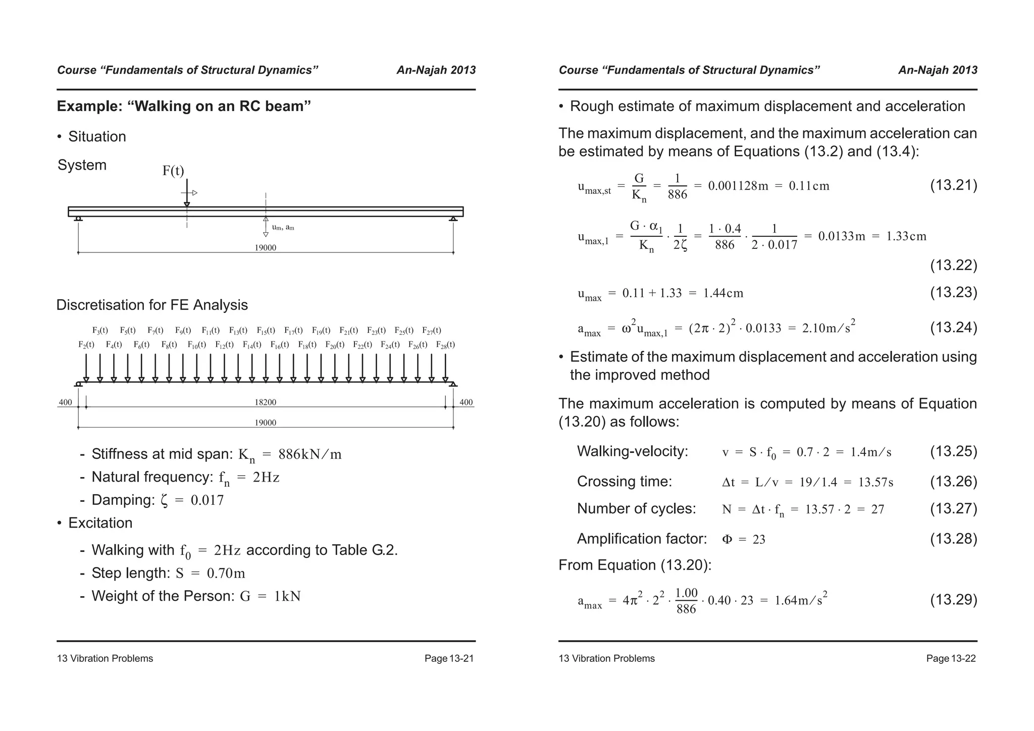
![Course “Fundamentals of Structural Dynamics” An-Najah 2013
13 Vibration Problems Page13-23
• Computation of displacements and accelerations by means of
the FE Programme ABAQUS
Displacements and accelerations are computed by means of
time-history analysis:
- Excitation
0.6
0.8
1
1.2
1.4
1.6
ce/Staticweight[-]
F1
F2
F3
F15
F28
0
0.2
0.4
0 2 4 6 8 10 12 14 16
Forc
Time [s]
Course “Fundamentals of Structural Dynamics” An-Najah 2013
13 Vibration Problems Page13-24
- Time history of the displacement
- Time history of the acceleration
-0.5
0
0.5
1
1.5
displacementum[cm]
Displacement at mid span
-1.5
-1
0 5 10 15 20 25 30 35 40
Vertical
Time [s]
-0.5
0
0.5
1
1.5
2
accelerationam[m/s2]
Acceleration at mid span
-2
-1.5
-1
0 5 10 15 20 25 30 35 40
Verticala
Time [s]](https://image.slidesharecdn.com/fundamentalsofstructuraldynamics-200730194708/75/Fundamentals-of-structural-dynamics-191-2048.jpg)
![Course “Fundamentals of Structural Dynamics” An-Najah 2013
13 Vibration Problems Page13-25
• Remarks
- The refined method and the time history calculations show
lower values compared to the rough method;
- The refined method and the time history calculations are in
good agreement;
- The time history of the displacement is not symmetric
compared to the time axis, because of the static compo-
nent of the displacement caused by the weigh of the cross-
ing person;
- The time history of the acceleration is symmetric com-
pared to the time axis, because there is no static compo-
nent of the acceleration.
• Swinging footbridge on the Internet
http://www.londonmillenniumbridge.com/
http://www.youtube.com
Course “Fundamentals of Structural Dynamics” An-Najah 2013
13 Vibration Problems Page13-26
13.3.4 Floors in residential and office buildings
• Frequency tuning
- If the excitation is generated by walking ( ), the
following natural frequencies shall be exceeded:
• Amplitude limitation
- Calculation of the acceleration maximum amplitude
(13.30)
- Because of the many non-structural components (wallpa-
per, furniture, suspended ceilings, technical floors, parti-
tions, ....) it is difficult to estimate the dynamic properties of
the floors.
- Where possible measure the dynamic properties.
Response of people to vibrations
The sensitivity of people to vibration depends on many parame-
ters:
Damping
Natural frequency
[Hz]
Remark
> 5% > 5
Avoid resonance due to the
second harmonic
< 5% > 7.5
Avoid resonance due to the
third harmonic
fmax 2.4Hz≅
amax ca. 0.05m s
2
⁄< 0.5% g=](https://image.slidesharecdn.com/fundamentalsofstructuraldynamics-200730194708/75/Fundamentals-of-structural-dynamics-192-2048.jpg)
![Course “Fundamentals of Structural Dynamics” An-Najah 2013
13 Vibration Problems Page13-27
- Position (standing, sitting, lying)
- Direction of the action compared to the spinal column
- Activity (resting, walking, running, ...)
- Type of vibration
- ....
• ISO 2631 standard
(13.31)
Where is the period of time over which the effective accelera-
tion was measured.
3 limits are defined:
- G1: Reduced comfort boundary
- G2: Fatigue-decreased proficiency boundary ~ 3 x G1
- G3: Exposure limit ~ 6 x G1
Description
Frequency 1 to 10 Hz
amax [m/s2
]
Frequency 10 to 100 Hz
vmax [m/s]
Barely noticeable
Clearly noticeable
Disturbing
Not tolerable
0.034
0.1
0.55
1.8
0.0005
0.0013
0.0068
0.0138
Vertical harmonic vibration action on a standing person. Accepted averages; scat-
ters up to a factor of 2 is possible (from [Bac+97])
aeff
1
T
--- a
2
t( ) td
0
T
³=
T
Course “Fundamentals of Structural Dynamics” An-Najah 2013
13 Vibration Problems Page13-28
• G2 limit for vibrations parallel to the spinal column
• G2 limit for vibrations transverse to the spinal column](https://image.slidesharecdn.com/fundamentalsofstructuraldynamics-200730194708/75/Fundamentals-of-structural-dynamics-193-2048.jpg)
![Course “Fundamentals of Structural Dynamics” An-Najah 2013
13 Vibration Problems Page13-29
13.3.5 Gyms and dance halls
Due to gymnastics or dancing, very large dynamic forces are
generated. This is readily understandable when the Fourier co-
efficients in Table G2 are considered:
- Walking: , ,
- Running: , ,
- Jumping: , ,
- Dancing: , ,
(however: a - many people moving rhythmically. b - certain
dances are very similar to jumping)
• Frequency tuning
- If the excitation is generated through jumping ( )
or dancing ( ), then the following natural frequen-
cies shall be exceeded:
Construction
Gyms
Natural frequency
[Hz]
Dance halls
Natural frequency
[Hz]
Reinforced concrete
Prestressed concrete
Composite structures
Steel
> 7.5
> 8.0
> 8.5
> 9.0
> 6.5
> 7.0
> 7.5
> 8.0
α1 0.4= α2 0.1= α3 0.1=
α1 1.6= α2 0.7= α3 0.2=
α1 1.9= α2 1.6= α3 1.1=
α1 0.5= α2 0.15= α3 0.1=
fmax 3.4Hz≅
fmax 3.0Hz≅
Course “Fundamentals of Structural Dynamics” An-Najah 2013
13 Vibration Problems Page13-30
• Amplitude limitation
- Calculation of the acceleration maximum amplitude
(13.32)
- Limits depend on the activity, if e.g. people are sitting in the
dance hall, as well, this limit shall be reduced.
- Because of the large forces that can be generated through
these activities, the dynamic characteristics of the structure
shall be estimated as precisely as possible.
13.3.6 Concert halls, stands and diving platforms
See [Bac+97].
13.4 Machinery induced vibrations
It is not possible to carry out here a detailed treatment of machin-
ery induced vibrations. Therefore, reference to [Bac+97] is
made.
amax ca. 0.5m s
2
⁄< 5% g=](https://image.slidesharecdn.com/fundamentalsofstructuraldynamics-200730194708/75/Fundamentals-of-structural-dynamics-194-2048.jpg)
![Course “Fundamentals of Structural Dynamics” An-Najah 2013
13 Vibration Problems Page13-31
13.5 Wind induced vibrations
Wind-induced vibrations cover a challenging and wide area. It is
not possible to carry out here their detailed treatment. Therefore,
reference is made to the relevant literature:
• [Bac+97]
• Simiu E., Scanlan R.H.: “Wind Effects on Structures”. Third
Edition. John Wiley & Sons, 1996.
13.5.1 Possible effects
• Gusts: Stochastic effects in wind direction
- Turbulent wind with spatially and temporally variable wind
speed.
Course “Fundamentals of Structural Dynamics” An-Najah 2013
13 Vibration Problems Page13-32
• Vortex shedding: Periodic action transversely to the wind di-
rection
- Vortex are not shedded left and right at the same time. If the
time-interval of the vortex shedding is equal to the oscilla-
tion period of the structure, resonance excitation occurs.
(13.33)
Where
: Critical wind velocity
: Natural frequency of the structure transverse to the
wind direction
: Diameter of the structure
: Strouhal number (about 0.2 for circular cross sections)
• Buffeting: Periodic action in wind direction
- Vortex detached from an obstacle hit the structure
ucrit
fe d⋅
S
-----------=
ucrit
fe
d
S](https://image.slidesharecdn.com/fundamentalsofstructuraldynamics-200730194708/75/Fundamentals-of-structural-dynamics-195-2048.jpg)
![Course “Fundamentals of Structural Dynamics” An-Najah 2013
13 Vibration Problems Page13-33
• “Gallopping” and “Flutter”:
Unstable interaction between wind flow and structural motion
- Gallopping: Motion of the structure transversely to the flow
direction.
- Flutter: Combined flexural-torsional motion of the structure.
Work done by wind forces during flutter
Stability curves for bridge cross-sections
Course “Fundamentals of Structural Dynamics” An-Najah 2013
13 Vibration Problems Page13-34
13.6 Tuned Mass Dampers (TMD)
13.6.1 Introduction
When discussing MDoF systems, in Section 11.1.3 a Tuned
Mass Damper (TMD) has already been discussed. However, in
that case zero damping was assumed for both the structure and
the TMD.
Here the theory of the TMD with damping is treated. As we shall
see, the damping of the two degrees of freedom is a design pa-
rameter, and it shall be possible to chose it freely, therefore:
• References
[BW95] Bachmann H., Weber B.: “Tuned Vibration Absorbers for
Damping of Lively Structures”. Structural Engineering Inter-
national, No. 1, 1995.
[Den85] Den Hartog J.P.: “Mechanical Vibrations”. ISBN 0-486-
64785-4. Dover Publications,1985. (Reprint of the original
fourth edition of 1956)
There it was possible to solve the equation of
motion simply by means of modal analysis.
In the case of TMD with damping
modal analysis can not be used](https://image.slidesharecdn.com/fundamentalsofstructuraldynamics-200730194708/75/Fundamentals-of-structural-dynamics-196-2048.jpg)
![Course “Fundamentals of Structural Dynamics” An-Najah 2013
13 Vibration Problems Page13-35
13.6.2 2-DoF system
The equations of motion of the 2-DoF system shown above are:
(13.34)
For an harmonic excitation of the type , a possi-
ble ansatz for the steady-state part of the solution is:
, , , (13.35)
Using the complex numbers formulation allows a particularly el-
egant solution to the problem. The equations of motion become:
mHu··
H cHu·
H cT u·
H u·
T–( ) kHuH kT uH uT–( )+ + + + F t( )=
mTu··
T cT u·
T u·
H–( ) kT uT uH–( )+ + 0=¯
®
F t( ) FH ωt( )cos=
uH UHe
iωt
= uT UTe
iωt
= F t( ) FHe
iωt
=
Course “Fundamentals of Structural Dynamics” An-Najah 2013
13 Vibration Problems Page13-36
(13.36)
To facilitate the solution of the system, some dimensionless pa-
rameters are now introduced:
: Mass ratio (TMD Mass/Mass of the structure)
: Natural frequency of the TMD
: Natural frequency of the structure without TMD
: Ratio of the natural frequencies
: Ratio of the excitation frequency to the natural
frequency of the structure
: Damping ratio of the TMD
: Damping ratio of the structure
: Static deformation of the structure
Substituting these dimensionless parameters into Equation
(13.36) we obtain:
(13.37)
ω
2
mH– iω cH cT+( ) kH kT+( )+ +[ ]UH iωcT– kT–[ ]UT+ FH=
iωcT– kT–[ ]UH ω
2
mT– iωcT kT+ +[ ]UT+ 0=
¯
°
®
°
γ mT mH⁄=
ωT kT mT⁄=
ωH kH mH⁄=
β ωT ωH⁄=
Ω ω ωH⁄=
ζT
ζH
UH0 FH kH⁄=
Ω
2
– 2iΩ ζH βγζT+( ) 1 β
2
γ+( )+ +[ ]UH 2iΩβγζT– β
2
γ–[ ]UT+ UH0=
2iΩβγζT– β
2
γ–[ ]UH Ω
2
γ– 2iΩβγζT β
2
γ+ +[ ]UT+ 0=
¯
°
®
°
](https://image.slidesharecdn.com/fundamentalsofstructuraldynamics-200730194708/75/Fundamentals-of-structural-dynamics-197-2048.jpg)
![Course “Fundamentals of Structural Dynamics” An-Najah 2013
13 Vibration Problems Page13-37
The system of equation can be easily solved using “Maple”, and
we obtain the following expression for the amplification function
:
(13.38)
The complex expression given in Equation (13.38) shall now be
converted into the form:
or (13.39)
The displacement has therefore two components: 1) One
that is in phase with the displacement and 2) one with a
phase shift equal to . From the vectorial sum of these two
components the norm of can be computed as:
(13.40)
Equation (13.38) has however the form
(13.41)
and must be first rearranged as follows:
(13.42)
(13.43)
UH UH0⁄
UH
UH0
---------
β
2
Ω
2
–( ) 2iΩβζT+
β
2
Ω
2
–( ) Ω
2
β
2
1 γ–( )– Ω
2
Ω
2
4βζHζT–( )+[ ] 2i β
2
Ω
2
–( )ζH 1 Ω
2
Ω
2
γ––( )βζT+[ ]+
-------------------------------------------------------------------------------------------------------------------------------------------------------------------------------------------------------------------=
z x iy+= UH UH0 x iy+( )=
UH
UH0
π 4⁄
UH
UH UH0 x
2
y
2
+=
UH UH0
A iB+( )
C iD+( )
---------------------=
UH UH0
A iB+( ) C iD–( )⋅
C iD+( ) C iD–( )⋅
----------------------------------------------- UH0
AC BD+( ) i BC AD–( )+
C
2
D
2
+
-----------------------------------------------------------------= =
UH UH0
A
2
B
2
+
C
2
D
2
+
-------------------=
Course “Fundamentals of Structural Dynamics” An-Najah 2013
13 Vibration Problems Page13-38
Thus, the norm of the dynamic amplification function
can be easily calculated:
(13.44)
A similar procedure can be followed to compute the dynamic am-
plification function .
Next figure show a representation of Equation (13.44) in function
of for an undamped structure . Curves for different val-
ues of the parameters , and are provided.
UH UH0⁄
UH
UH0
---------
β
2
Ω
2
–( )
2
2ΩβζT( )
2
+
β
2
Ω
2
–( ) Ω
2
β
2
1 γ–( )– Ω
2
Ω
2
4βζHζT–( )+[ ]
2
4 β
2
Ω
2
–( )ζH 1 Ω
2
Ω
2
γ––( )βζT+[ ]
2
+
---------------------------------------------------------------------------------------------------------------------------------------------------------------------------------------------------------------------=
UT UH0⁄
Ω ζH 0=
β γ ζT
0
4
8
12
16
0.6 0.7 0.8 0.9 1 1.1 1.2 1.3
: [-]
UH/UH0[-]
]T=0 ]T=inf.
]T=0.10
]T=0.32
P
Q
J = 1/20
E = 1](https://image.slidesharecdn.com/fundamentalsofstructuraldynamics-200730194708/75/Fundamentals-of-structural-dynamics-198-2048.jpg)
![Course “Fundamentals of Structural Dynamics” An-Najah 2013
13 Vibration Problems Page13-39
13.6.3 Optimum TMD parameters
Based on observations and consideration at the previous image
Den Hartog found optimum TMD parameters for an undamped
structure:
or (13.45)
(13.46)
These optimum TMD parameters can be applied also to lowly
damped structures providing good response results.
13.6.4 Important remarks on TMD
• The frequency tuning of the TMD shall be quite precise
• The compliance with the optimum damping is less important
• Design charts for TMDs shall be computed numerically
• TMDs are most effective when the damping of the structure is low
• It is not worth increasing the mass ratio too much
• For large mass ratios, the amplitude of the TMD oscillations reduce
• Meaningful mass ratios are 3-5%
• The exact tuning of the TMD occurs experimentally, therefore
great care should be paid to construction details.
fT opt,
fH
1 mT mH⁄+
-----------------------------
fH
1 γ+
-----------= = βopt
1
1 γ+
-----------=
ζT opt,
3mT mH⁄
8 1 mT mH⁄+( )
3
---------------------------------------
3γ
8 1 γ+( )
3
----------------------= =
γ
Course “Fundamentals of Structural Dynamics” An-Najah 2013
13 Vibration Problems Page13-40
• Amplification function with TMD: Variation of TMD frequency
• Amplification function with TMD: Variation of TMD damping
20
30
40
50
UH/UH0[-]
No TMD (ζT=inf.)
γ = 0.01
ζΗ = 0.01
fT=0.98fT,optfT=1.02fT opt
0
10
0.6 0.7 0.8 0.9 1 1.1 1.2 1.3
Ω [-]
fT=fT,opt
fT 1.02fT,opt
20
30
40
50
UH/UH0[-]
No TMD (ζT=inf.)
γ = 0.01
ζΗ = 0.01
ζT=1 5ζT t
ζT=0.5ζT opt
0
10
0.6 0.7 0.8 0.9 1 1.1 1.2 1.3
Ω [-]
ζT 1.5ζT,opt
ζT=ζT,opt
ζT 0 5ζT,opt](https://image.slidesharecdn.com/fundamentalsofstructuraldynamics-200730194708/75/Fundamentals-of-structural-dynamics-199-2048.jpg)
![Course “Fundamentals of Structural Dynamics” An-Najah 2013
13 Vibration Problems Page13-41
• Design charts: Displacement of the structure (from [BW95])
• Design charts: Relative TMD displacement (from [BW95])
Course “Fundamentals of Structural Dynamics” An-Najah 2013
13 Vibration Problems Page13-42
Blank page](https://image.slidesharecdn.com/fundamentalsofstructuraldynamics-200730194708/75/Fundamentals-of-structural-dynamics-200-2048.jpg)
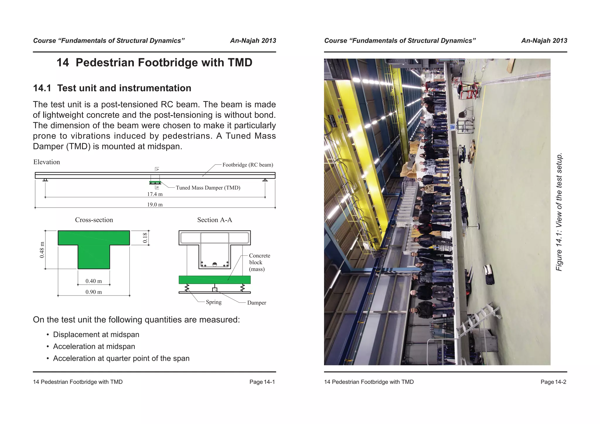
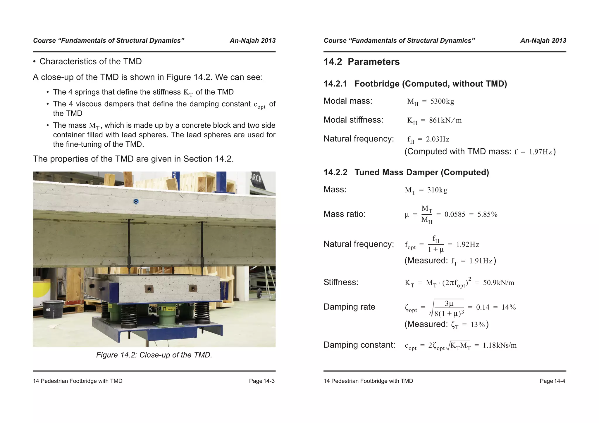
![Course “Fundamentals of Structural Dynamics” An-Najah 2013
14 Pedestrian Footbridge with TMD Page14-5
14.3 Test programme
Following tests are carried out:
Typical results of the experiments are presented and briefly
commented in the following sections.
No. Test Action location TMD
1 Free decay Midspan Locked
2 Sandbag Midspan Locked
3 Sandbag Quarter-point Locked
4 Sandbag Midspan Free
5 Walking 1 Person 3Hz Along the beam Locked
6 Walking 1 Person 2Hz Along the beam Locked
7 Walking 1 Person 2Hz Along the beam Free
8 Walking in group 2Hz Along the beam Locked
9 Walking in group 2Hz Along the beam Free
10 Jumping 1 Person 2Hz Midspan Locked
11 Jumping 1 Person 2Hz Midspan Free
Course “Fundamentals of Structural Dynamics” An-Najah 2013
14 Pedestrian Footbridge with TMD Page14-6
14.4 Free decay test with locked TMD
Time history of the displacement at midspan
Evaluation:
Figure 14.3: Free decay test with locked TMD: Displacement at
midspan.
Logarithmic
decrement
Damping ratio
Region 1
Average amplitude: ~30mm
Region 2
Average amplitude: ~14mm
Region 3
Average amplitude: ~6mm
0 5 10 15 20
Time [s]
-40
-30
-20
-10
0
10
20
30
40
Displacementatmidspan[mm]
δ
1
8
--- 41.36
21.66
-------------ln 0.081= = ζH
0.081
2π
------------- 1.29%= =
δ
1
8
--- 19.91
9.68
-------------ln 0.090= = ζH
0.090
2π
------------- 1.43%= =
δ
1
8
--- 8.13
3.90
----------ln 0.092= = ζH
0.092
2π
------------- 1.46%= =](https://image.slidesharecdn.com/fundamentalsofstructuraldynamics-200730194708/75/Fundamentals-of-structural-dynamics-203-2048.jpg)
![Course “Fundamentals of Structural Dynamics” An-Najah 2013
14 Pedestrian Footbridge with TMD Page14-7
Fourier-spectrum of the displacement at midspan
The measured natural frequency of the footbridge with locked
TMD is equal to:
(14.1)
This value is less than the value given in Section 14.2.1. This
can be explained with the large amplitude of vibration at the start
of the test, which causing the opening of cracks in the web of the
beam, hence reducing its stiffness.
The second peak in the spectrum corresponds to ,
wich is in good agreement with Section 14.2.1.
Figure 14.4: Free decay test with locked TMD: Fourier-spectrum of the
displacement at midspan.
0.0 0.5 1.0 1.5 2.0 2.5 3.0 3.5 4.0
Frequency [Hz]
0.0
0.5
1.0
1.5
2.0
"Spectraldisplacement"
f 1.89Hz=
f 1.98Hz=
Course “Fundamentals of Structural Dynamics” An-Najah 2013
14 Pedestrian Footbridge with TMD Page14-8
14.5 Sandbag test
The sandbag test consists in hanging a 20 kg sandbag 1 meter
above the footbridge, letting it fall down and measuring the re-
sponse of the system.
In order to excite the different modes of vibration of the foot-
bridge, the test is repeated several times changing the position
of the impact of the sandbag on the bridge. The considered lo-
cations are:
- at midspan (Section 14.5.1)
- at quarter-point of the span (Section 14.5.2).
These tests are carried out with locked TMD. In order to investi-
gate the effect of the TMD on the vibrations of the system, the
test of Section 14.5.1 is repeated with free TMD (see Section
14.5.3).
Remark
• The results presented in Section 14.5.1 and those presented
in Section 14.5.2 and 14.5.3 belongs to two different series of
tests carried out at different point in time. Between these test
series the test setup was completely disassembled and reas-
sembled. Slight differences in the assemblage of the test setup
(support!) may have led to slightly different natural frequencies
of the system.](https://image.slidesharecdn.com/fundamentalsofstructuraldynamics-200730194708/75/Fundamentals-of-structural-dynamics-204-2048.jpg)
![Course “Fundamentals of Structural Dynamics” An-Najah 2013
14 Pedestrian Footbridge with TMD Page14-9
14.5.1 Locked TMD, Excitation at midspan
Figure 14.5: Sandbag test with locked TMD: Acceleration at midspan.
Figure 14.6: Sandbag test with locked TMD: Fourier-spectrum of the
acceleration at midspan.
0 1 2 3 4 5 6 7 8 9 10
Time [s]
-1.0
-0.5
0.0
0.5
1.0
Accelerationanmidspan[m/s2
]
0 5 10 15 20
Frequency [Hz]
0.000
0.010
0.020
0.030
0.040
"Spectralacceleration"
f1=2.00Hz
f3=18.06Hz
Course “Fundamentals of Structural Dynamics” An-Najah 2013
14 Pedestrian Footbridge with TMD Page14-10
Figure 14.7: Sandbag test with locked TMD: Acceleration at quarter-
point of the span.
Figure 14.8: Sandbag test with locked TMD: Fourier-spectrum of the
acceleration at quarter-point of the span.
0 1 2 3 4 5 6 7 8 9 10
Time [s]
-1.0
-0.5
0.0
0.5
1.0
Acc.atquarter-point[m/s2
]
0 5 10 15 20
Frequency [Hz]
0.000
0.010
0.020
0.030
0.040
"Spectralacceleration"
f1=2.00Hz
f3=18.06Hz](https://image.slidesharecdn.com/fundamentalsofstructuraldynamics-200730194708/75/Fundamentals-of-structural-dynamics-205-2048.jpg)
![Course “Fundamentals of Structural Dynamics” An-Najah 2013
14 Pedestrian Footbridge with TMD Page14-11
Remarks
• With the sandbag test in principle all frequencies can be excit-
ed. Figures 14.5 and 14.7 show a high-frequency vibration,
which is superimposed on a fundamental vibration;
• The Fourier amplitude spectrum shows prominent peaks at the
first and third natural frequencies of the system (Footbridge
with locked TMD);
• The second mode of vibration of the system is not excited, be-
cause the sandbag lands in a node of the second eigenvector.
• At midspan, the amplitude of the vibration due to the first mode
of vibration is greater than at quarter-point. The amplitude of
the vibration due to the third mode of vibration, however, is
about the same in both places. This is to be expected, if the
shape of the first and third eigenvectors is considered.
• The vibration amplitude is relatively small, therefore, the meas-
ured first natural frequency in good agreement with
the computation provided in Section 14.2.1.
f1 2.0Hz=
Course “Fundamentals of Structural Dynamics” An-Najah 2013
14 Pedestrian Footbridge with TMD Page14-12
14.5.2 Locked TMD, Excitation at quarter-point of the span
Figure 14.9: Sandbag test with locked TMD: Acceleration at midspan.
Figure 14.10: Sandbag test with locked TMD: Fourier-spectrum of the
acceleration at midspan.
0 1 2 3 4 5 6 7 8 9 10
Time [s]
-1.0
-0.5
0.0
0.5
1.0
Accelerationatmidspan[m/s2
]
0 5 10 15 20
Frequency [Hz]
0.000
0.010
0.020
0.030
0.040
"Spectralacceleration"
f1=2.00Hz
f3=18.31Hz](https://image.slidesharecdn.com/fundamentalsofstructuraldynamics-200730194708/75/Fundamentals-of-structural-dynamics-206-2048.jpg)
![Course “Fundamentals of Structural Dynamics” An-Najah 2013
14 Pedestrian Footbridge with TMD Page14-13
Figure 14.11: Sandbag test with locked TMD: Acceleration at quarter-
point of the span.
Figure 14.12: Sandbag test with locked TMD: Fourier-spectrum of the
acceleration at quarter-point of the span.
0 1 2 3 4 5 6 7 8 9 10
Time [s]
-1.0
-0.5
0.0
0.5
1.0
Acc.atquarter-point[m/s2
]
0 5 10 15 20
Frequency [Hz]
0.000
0.010
0.020
0.030
0.040
"Spectralacceleration"
f1=2.00Hz
f3=18.31Hz
f2=8.84Hz
Course “Fundamentals of Structural Dynamics” An-Najah 2013
14 Pedestrian Footbridge with TMD Page14-14
Remarks
• When the sandbag lands at quarter-point of the bridge, the
second mode of vibration of the system is strongly excited. Its
contribution to the overall vibration at quarter-point of the foot-
bridge is clearly shown in Figures 14.11 and 14.12.
• The acceleration sensor located at midspan of the footbridge
lays in a node of the second mode of vibration, and as expect-
ed in figures 14.9 and 14.10 the contribution of the second
mode is vanishingly small.](https://image.slidesharecdn.com/fundamentalsofstructuraldynamics-200730194708/75/Fundamentals-of-structural-dynamics-207-2048.jpg)
![Course “Fundamentals of Structural Dynamics” An-Najah 2013
14 Pedestrian Footbridge with TMD Page14-15
14.5.3 Free TMD: Excitation at midspan
Figure 14.13: Sandbag test with free TMD: Acceleration at midspan.
Figure 14.14: Sandbag test with free TMD: Fourier-spectrum of the
acceleration at midspan.
0 1 2 3 4 5 6 7 8 9 10
Time [s]
-1.0
-0.5
0.0
0.5
1.0
Accelerationatmidspan[m/s2
]
0 5 10 15 20
Frequency [Hz]
0.000
0.010
0.020
0.030
0.040
"Spectralacceleration"
“f1=2.05Hz”
“f3=19.04Hz”
Course “Fundamentals of Structural Dynamics” An-Najah 2013
14 Pedestrian Footbridge with TMD Page14-16
Remarks
• With active (free) TMD the “first” and the “third “natural fre-
quencies of the bridge are excited. As expected, these fre-
quencies are slightly larger than the natural frequencies of the
system (bridge with locked TMD), which are given in Figure
14.6. This is because the mass of the TMD is no longer locked
and can vibrate freely.
• The effect of the TMD is clearly shown in Figure 14.14. The
amplitude of the peak in the “first natural frequency” is much
smaller than in Figure 14.6. The amplitude of the peak at the
“third natural frequency” is practically the same. The “third
mode of vibration” is only marginally damped by the TMD.
• In the two comments above, the natural frequencies are men-
tioned in quotes, because by releasing the TMD number and
properties of the natural vibrations of the system change. A di-
rect comparison with the natural vibrations of system with
locked TMD is only qualitatively possible.](https://image.slidesharecdn.com/fundamentalsofstructuraldynamics-200730194708/75/Fundamentals-of-structural-dynamics-208-2048.jpg)
![Course “Fundamentals of Structural Dynamics” An-Najah 2013
14 Pedestrian Footbridge with TMD Page14-17
14.6 One person walking with 3 Hz
One 65 kg-heavy person (G = 0.64 kN) crosses the footbridge.
He walks with a frequency of about 3 Hz, which is significantly
larger than the first natural frequency of the bridge.
Remarks
• The static deflection of the bridge when the person stands at
midspan is:
• The maximum measured displacement at midspan of the
bridge is about 2 mm (see Figure 14.15), which corresponds to
about 2.5 times . As expected, the impact of dynamic effects
is rather small.
• In the Fourier spectrum of the acceleration at midspan of the
bridge (see Figure 14.17), the frequencies that are represent-
ed the most correspond to the first, the second and the third
harmonics of the excitation. However, frequencies correspond-
ing to the natural modes of vibrations of the system are also
visible.
dst
G
KH
-------
0.69
861
---------- 0.00080m 0.80mm= = = =
dst
Course “Fundamentals of Structural Dynamics” An-Najah 2013
14 Pedestrian Footbridge with TMD Page14-18
Test results
Figure 14.15: One person walking with 3 Hz: Displacement at midspan
with locked TMD.
Figure 14.16: One person walking with 3 Hz: Acceleration at midspan
with locked TMD.
0 5 10 15 20 25 30 35 40
Time [s]
-2.0
-1.0
0.0
1.0
2.0
Displacementatmidspan[mm]
0 5 10 15 20 25 30 35 40
Time [s]
-1.0
-0.5
0.0
0.5
1.0
Accelerationatmidspan[m/s2
]](https://image.slidesharecdn.com/fundamentalsofstructuraldynamics-200730194708/75/Fundamentals-of-structural-dynamics-209-2048.jpg)
![Course “Fundamentals of Structural Dynamics” An-Najah 2013
14 Pedestrian Footbridge with TMD Page14-19
Figure 14.17: One person walking with 3 Hz: Fourier-Spectrum of the
acceleration at midspan with locked TMD.
0 5 10 15 20
Frequency [Hz]
0.000
0.005
0.010
0.015
"Spectralacceleration"
Course “Fundamentals of Structural Dynamics” An-Najah 2013
14 Pedestrian Footbridge with TMD Page14-20
14.7 One person walking with 2 Hz
One 95 kg-heavy person (G = 0.93 kN) crosses the footbridge. He
walks with a frequency of 1.95 Hz, which is approximately equal to the
first natural frequency of the bridge. The length of the step is 0.70 m.
Sought is the response of the bridge under this excitation. A
similar problem was solved theoretically in Section 13.3.3.
14.7.1 Locked TMD (Measured)
First the maximum amplitudes are calculated by hand:
Static displacement:
(Measured: )
Walking velocity:
Crossing time:
Number of cycles:
Amplification factor: (From page 13-20 with )
Max. acceleration:
(Measured: )
Max. dyn. displ.:
Max. displacement:
(Measured: )
dst
G
KH
-------
0.93
861
---------- 0.00108m 1.08mm= = = =
dst 1.22mm=
v S f0⋅ 0.7 1.95⋅ 1.365m s⁄= = =
Δt L v⁄ 17.40 1.365⁄ 12.74s= = =
N Δt fn⋅ 12.74 1.95⋅ 25= = =
Φ 22= ζH 1.6%=
amax 4π
2
1.95
2
0.00108 0.4 22⋅ ⋅ ⋅ ⋅
1.43m s2⁄
=
=
amax 1.63m s2⁄=
ddyn,max 1.08 0.4 22⋅ ⋅ 9.50mm= =
dmax 9.50 1.08+ 10.58mm= =
dmax 12.04mm=](https://image.slidesharecdn.com/fundamentalsofstructuraldynamics-200730194708/75/Fundamentals-of-structural-dynamics-210-2048.jpg)
![Course “Fundamentals of Structural Dynamics” An-Najah 2013
14 Pedestrian Footbridge with TMD Page14-21
Test results
Figure 14.18: One person walking with 2 Hz: Displacement at midspan
with locked TMD.
Figure 14.19: One person walking with 2 Hz: Acceleration at midspan
with locked TMD.
0 5 10 15 20 25 30 35 40
Time [s]
-10
-5
0
5
10
Displacementatmidspan[mm]
0 5 10 15 20 25 30 35 40
Time [s]
-2.0
-1.5
-1.0
-0.5
0.0
0.5
1.0
1.5
2.0
Accelerationatmidspan[m/s2
]
Course “Fundamentals of Structural Dynamics” An-Najah 2013
14 Pedestrian Footbridge with TMD Page14-22
14.7.2 Locked TMD (ABAQUS-Simulation)
Figure 14.20: One person walking with 2 Hz: Displacement at midspan
with locked TMD. (ABAQUS-Simulation).
Figure 14.21: One person walking with 2 Hz: Acceleration at midspan
with locked TMD. (ABAQUS-Simulation).
0 5 10 15 20 25 30 35 40
Time [s]
-10
-5
0
5
10
Displacementatmidspan[mm]
0 5 10 15 20 25 30 35 40
Time [s]
-2.0
-1.5
-1.0
-0.5
0.0
0.5
1.0
1.5
2.0
Accelerationatmidspan[m/s2
]](https://image.slidesharecdn.com/fundamentalsofstructuraldynamics-200730194708/75/Fundamentals-of-structural-dynamics-211-2048.jpg)
![Course “Fundamentals of Structural Dynamics” An-Najah 2013
14 Pedestrian Footbridge with TMD Page14-23
The curves in Figures 14.20 and 14.21 were computed using the
FE program ABAQUS. A similar calculation is described in detail
in Section 13.3.3. The input data used in that section were only
slightly adjusted here in order to better describe the properties of
the test.
Maximum vibration amplitude
Static displacement:
(Measured: )
Maximum displacement:
(Measured: )
Amplification factor:
Maximum acceleration:
(Measured: )
The maximum amplitudes of the numerical simulation and of the
experiment agree quite well and also the time-histories shown in
Figures 14.18 and 14.21 look quite similar.
Please note that during the first 2 seconds of the experiment,
displacements and accelerations are zero, because the person
started to walk with a slight delay.
dst 1.08mm=
dst 1.22mm=
dmax 11.30mm=
dmax 12.04mm=
V
dmax
dst
-----------
11.30
1.08
------------- 10.5= = =
amax 1.68m s2⁄=
amax 1.63m s2⁄=
Course “Fundamentals of Structural Dynamics” An-Najah 2013
14 Pedestrian Footbridge with TMD Page14-24
14.7.3 Free TMD
Figure 14.22: One person walking with 2 Hz: Displacement at midspan
with free TMD.
Figure 14.23: One person walking with 2 Hz: Acceleration at midspan
with free TMD.
0 5 10 15 20 25 30 35 40
Time [s]
-10
-5
0
5
10
Displacementatmidspan[mm]
0 5 10 15 20 25 30 35 40
time [s]
-2.0
-1.5
-1.0
-0.5
0.0
0.5
1.0
1.5
2.0
Accelerationatmidspan[m/s2
]](https://image.slidesharecdn.com/fundamentalsofstructuraldynamics-200730194708/75/Fundamentals-of-structural-dynamics-212-2048.jpg)
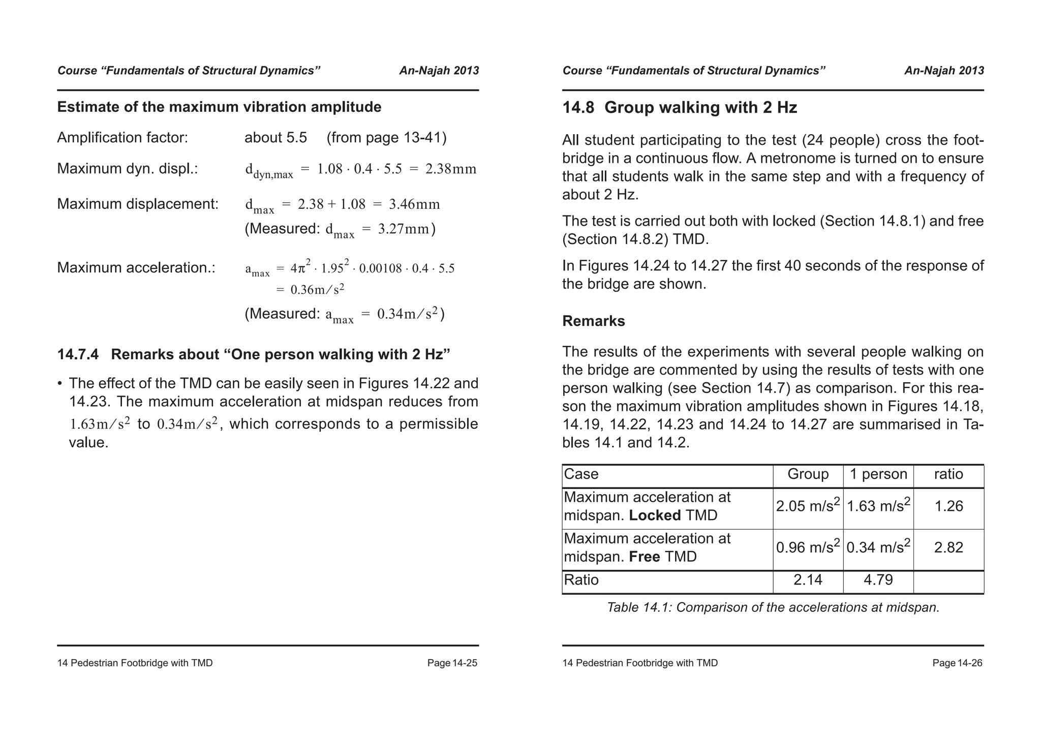
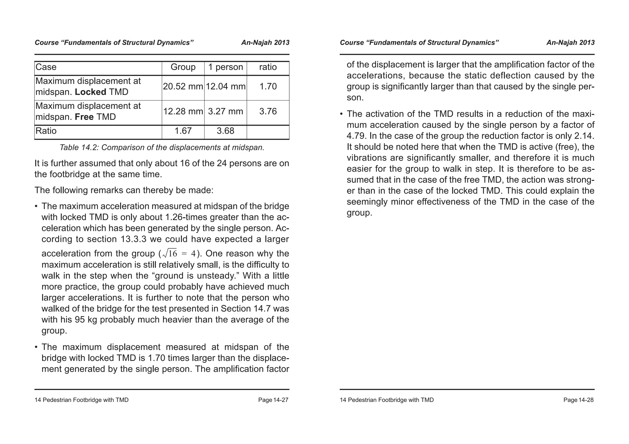
![Course “Fundamentals of Structural Dynamics” An-Najah 2013
14 Pedestrian Footbridge with TMD Page14-29
14.8.1 Locked TMD
Figure 14.24: Group walking with 2 Hz: Displacement at midspan with
locked TMD.
Figure 14.25: Group walking with 2 Hz: Acceleration at midspan with
locked TMD.
0 5 10 15 20 25 30 35 40
Time [s]
-20
-10
0
10
Displacementatmidspan[mm]
0 5 10 15 20 25 30 35 40
time [s]
-2.0
-1.0
0.0
1.0
2.0
Accelerationatmidspan[m/s2
]
Course “Fundamentals of Structural Dynamics” An-Najah 2013
14 Pedestrian Footbridge with TMD Page14-30
14.8.2 Free TMD
Figure 14.26: Group walking with 2 Hz: Displacement at midspan with
free TMD.
Figure 14.27: Group walking with 2 Hz: Acceleration at midspan with
free TMD.
0 5 10 15 20 25 30 35 40
Time [s]
-20
-10
0
10
Displacementatmidspan[mm]
0 5 10 15 20 25 30 35 40
Time [s]
-2.0
-1.0
0.0
1.0
2.0
Accelerationatmidspan[m/s2
]](https://image.slidesharecdn.com/fundamentalsofstructuraldynamics-200730194708/75/Fundamentals-of-structural-dynamics-215-2048.jpg)
![Course “Fundamentals of Structural Dynamics” An-Najah 2013
14 Pedestrian Footbridge with TMD Page14-31
14.9 One person jumping with 2 Hz
One 72 kg-heavy person (G = 0.71 kN) keeps jumping at mid-
span of the footbridge. He is jumping with a frequency of
1.95 Hz, which is approximately equal to the first natural fre-
quency of the bridge.
Sought is the response of the bridge under this excitation. A
similar problem was solved theoretically in Section 6.1.3.
14.9.1 Locked TMD
First the maximum amplitudes are calculated by hand:
Static displacement:
(Measured: )
Amplification factor:
Maximum acceleration:
(Measured: )
Max. dyn. displacement:
Maximum displacement:
(Measured: )
dst
G
KH
-------
0.71
861
---------- 0.0008m 0.82mm= = = =
dst 0.93mm=
V
1
2ζ
------
1
2 0.016⋅( )
------------------------- 31.25= = =
amax 4π
2
1.95
2
0.0008 1.8 31.25⋅ ⋅ ⋅ ⋅
6.92m s2⁄
=
=
amax 7.18m s2⁄=
ddyn,max 0.82 1.8 31.25⋅ ⋅ 46.13mm= =
dmax 46.13 0.82+ 46.95mm= =
dmax 51.08mm=
Course “Fundamentals of Structural Dynamics” An-Najah 2013
14 Pedestrian Footbridge with TMD Page14-32
Test results
Figure 14.28: One person jumping with 2 Hz: Displacement at midspan
with locked TMD.
Figure 14.29: One person jumping with 2 Hz: Acceleration at midspan
with locked TMD.
0 5 10 15 20 25 30 35 40
Time [s]
-60
-40
-20
0
20
40
60
Displacementatmidspan[mm]
0 5 10 15 20 25 30 35 40
Time [s]
-8.0
-6.0
-4.0
-2.0
0.0
2.0
4.0
6.0
8.0
Accelerationatmidspan[m/s2
]](https://image.slidesharecdn.com/fundamentalsofstructuraldynamics-200730194708/75/Fundamentals-of-structural-dynamics-216-2048.jpg)
![Course “Fundamentals of Structural Dynamics” An-Najah 2013
14 Pedestrian Footbridge with TMD Page14-33
14.9.2 Free TMD
Figure 14.30: One person jumping with 2 Hz: Displacement at midspan
with free TMD.
Figure 14.31: One person jumping with 2 Hz: Acceleration at midspan
with free TMD.
0 5 10 15 20 25 30 35 40
Time [s]
-60
-40
-20
0
20
40
60
Displacementatmidspan[mm]
0 5 10 15 20 25 30 35 40
Time [s]
-8.0
-6.0
-4.0
-2.0
0.0
2.0
4.0
6.0
8.0
Accelerationatmidspan[m/s2
]
Course “Fundamentals of Structural Dynamics” An-Najah 2013
14 Pedestrian Footbridge with TMD Page14-34
Estimate of the maximum vibration amplitude
Amplification factor: about 5.5 (from page 13-41)
Maximum dyn. displ.:
Maximum displacement:
(Measured: )
Maximum acceleration:
(Measured: )
14.9.3 Remarks about “One person jumping with 2 Hz”
• When jumping, the footbridge can be much strongly excited
than when walking.
• The achieved acceleration is very
large and two jumping people could easily produce the lift-off
of the footbridge.
• The effect of the TMD can be easily seen in Figures 14.30 and
14.31. The maximum acceleration at midspan reduces from
to , what, however, is still perceived as un-
pleasant.
ddyn,max 0.82 1.8 5.5⋅ ⋅ 8.12mm= =
dmax 8.12 0.82+ 8.94mm= =
dmax 8.12mm=
amax 4π
2
1.95
2
0.0008 1.8 5.5⋅ ⋅ ⋅ ⋅
1.22m s2⁄
=
=
amax 1.04m s2⁄=
amax 7.18m s2⁄ 73% g= =
7.18m s2⁄ 1.04m s2⁄](https://image.slidesharecdn.com/fundamentalsofstructuraldynamics-200730194708/75/Fundamentals-of-structural-dynamics-217-2048.jpg)

This document provides an overview of the course "Fundamentals of Structural Dynamics" to be held from April 19-23, 2013 at An-Najah National University. The course will cover topics related to single-degree-of-freedom and multi-degree-of-freedom structural systems including modeling, free vibration, forced vibration, seismic excitation, and response spectrum analysis. It will include theoretical background, example problems, and the use of software tools like MATLAB for dynamic analysis. Assignments will be given each day and the schedule outlines the daily topics to be covered over the five day period.


![Geotechnical Engineering-II [Lec #9+10: Westergaard Theory]](https://cdn.slidesharecdn.com/ss_thumbnails/9-181020124827-thumbnail.jpg?width=640&height=640&fit=bounds)


![Doubly reinforced beam]](https://cdn.slidesharecdn.com/ss_thumbnails/doublyreinforcedbeam-190218110616-thumbnail.jpg?width=640&height=640&fit=bounds)


![Geotechnical Engineering-II [Lec #7: Soil Stresses due to External Load]](https://cdn.slidesharecdn.com/ss_thumbnails/7-180930132739-thumbnail.jpg?width=640&height=640&fit=bounds)


