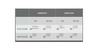
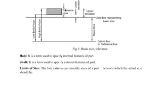
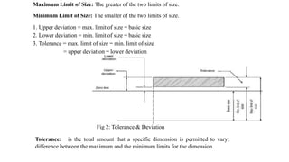
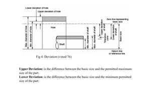
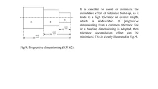
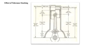
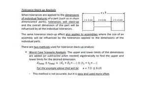
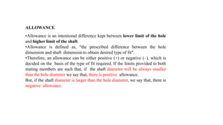
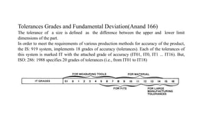
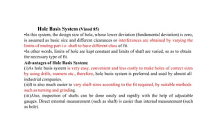
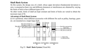
Module 2 part i limits, fits, and tolerances

Limits, Fits, and Tolerances
Introduction
• No two parts can be produced with identical measurements by any manufacturing process.
• In any production process, regardless of how well it is designed or how carefully it is
maintained, a certain amount of natural variability will always exist.
• These natural variations are random in nature and are the cumulative effect of many small,
essentially uncontrollable causes.
• Usually, variability arises from improperly adjusted machines, operator error, tool wear,
and/or defective raw materials (ppt, KM58).
• To satisfy the ever-increasing demand for accuracy, the parts have to be produced with less
dimensional variation. Hence, the labour and machinery required to manufacture a part has
become more expensive. It is essential for the manufacturer to have an in-depth knowledge
of the tolerances to manufacture parts economically.

The proper functioning of a manufactured product for a designed life depends upon its correct
size relationship between the various components of the assembly. This means that components
must fit with each other in the required fashion. (For example, if the shaft is to slide in a hole,
there must be enough clearance between the shaft and the hole to allow the oil film to be
maintained for lubrication).
If the clearance between two parts is too small, it may lead to seize of components. And if
clearance is too large, there would be vibration and rapid wear ultimately leading to failure.
To achieve the required conditions, the components must be produced with exact dimensions
specified at the design stage in part drawing.
Every production process involves mainly three elements, viz., man, machine and materials
(tool and job material). Each of these has some natural (inherent) variations, which are due
to chance causes and are difficult to trace and control, as well as some unnatural variations
which are due to assignable causes and can be systematically traced and controlled. Hence,
it is very difficult to produce extremely similar or identical (sized) components.

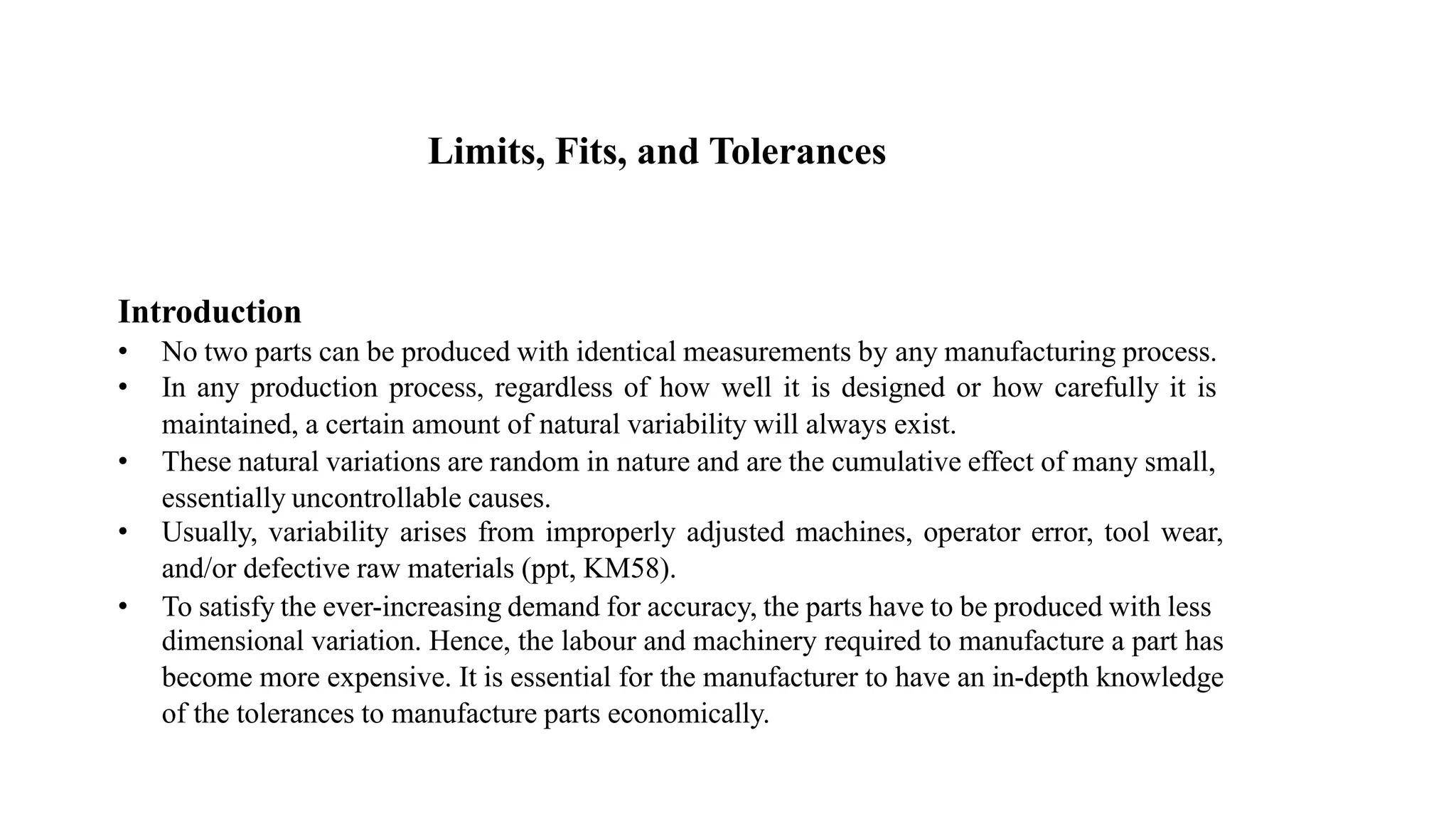
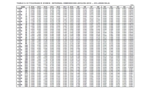
PRINCIPLE OF INTERCHANGEABILITY
Modern production techniques require that a complete product be broken into various component
parts so that the production of each part becomes an independent process, leading to
specialization.
When interchangeable manufacture is adopted, any one component selected at random should
assemble with any other arbitrarily chosen mating component. In order to assemble with a
predetermined fit, the dimensions of the components must be confined within the permissible
tolerance limits. By interchangeable assembly, we mean that identical components, manufactured
by different operators, using different machine tools and under different environmental
conditions, can be assembled and replaced without any further modification during the assembly
stage and without affecting the functioning of the component when assembled.
When one component assembles properly (and which
satisfies the functionality aspect of the assembly/product)
with any mating component, both chosen at random, then it
is known as interchangeability [Anand.150]

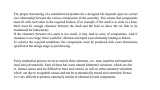
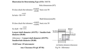
For example, consider the assembly of a shaft and a part with a hole. The two mating parts
are produced in bulk, say 1000 each. By interchangeable assembly any shaft chosen
randomly should assemble with any part with a hole selected at random, providing the
desired fit.
Another major advantage of interchangeability is the ease with which replacement of
defective or worn-out parts is carried out, resulting in reduced maintenance cost.
In order to achieve interchangeability, certain standards need to be followed, based on which
interchangeability can be categorized into two types—universal interchangeability and local
interchangeability.
When the parts that are manufactured at different locations are randomly chosen for assembly, it
is known as universal interchangeability. To achieve universal interchangeability, it is desirable
that common standards be followed by all and the standards used at various manufacturing
locations be traceable to international standards[Km51].
When the parts that are manufactured at the same manufacturing unit are randomly drawn for
assembly, it is referred to as local interchangeability. In this case, local standards are followed.

TERMINOLOGY
Basic size: It is the specified standard size of a part, with reference to which, all the limits of
variations of size are determined. It is same for both hole and its corresponding mating member
i.e. shaft. As basic size is specified before the production or inspection, it is also called as true
value.
Actual size: It is the actual measured value of manufactured job after measurement. Therefore,
it is also called as measured value.
Zero Line: In a graphical representation of limits and fits, a zero line is a straight line to which
the deviations are referred to. It is a line of zero deviation and represents the basic size. When
the zero line is drawn horizontally, positive deviations are shown above and negative deviations
are shown below this line.
Line corresponding to basic size is called as zero line. It is the line of zero deviation.

Hole: It is a term used to specify internal features of part.
Shaft: It is a term used to specify external features of part.
Limits of Size: The two extreme permissible sizes of a part between which the actual size
should lie.
Fig 1: Basic size, tolerance

Tolerance: is the total amount that a specific dimension is permitted to vary;
difference between the maximum and the minimum limits for the dimension.
Fig 2: Tolerance & Deviation
Maximum Limit of Size: The greater of the two limits of size.
Minimum Limit of Size: The smaller of the two limits of size.
1. Upper deviation = max. limit of size − basic size
2. Lower deviation = min. limit of size − basic size
3. Tolerance = max. limit of size − min. limit of size
= upper deviation − lower deviation

Tolerance is the algebraic difference between the maximum limit and minimum limit of a hole
or shaft.
•It is also defined as ‘difference between upper deviation and lower deviation'. It has an
absolute value without algebraic sign. (Neither plus or minus)
Tolerance can also be specified/defined as, "the amount, by which, the job is allowed to go
away from accuracy and perfectness without causing any functional trouble, when assembled
with mating part and the assembly is put into actual services".
• A shaft of dimension 25± 0.02 indicates that, Upper limit = 25.02 mm and Lower limit =
24.98 mm. Therefore, Tolerance zone = 25.02 – 24.98 = 0.04 mm.
Deviation: Deviation is the amount, by which, the actual size of a manufactured part deviates
from its basic size. Thus, deviation is the algebraic difference between actual size and basic
size.

Fig 3: Conventional diagram (anand 153 n ppt)
Fig 3: Deviation (vinod 76, ppt )

Upper Deviation: is the difference between the basic size and the permitted maximum
size of the part.
Lower Deviation: is the difference between the basic size and the minimum permitted
size of the part.
Fig 4: Deviation (vinod 76)

Fundamental deviation (FD) (Anand 155)
In fact, it is the upper or lower deviation, which is nearest to zero line, either for shaft or a hole.
Classification of Tolerance
Tolerance can be classified under the following categories:
1. Unilateral tolerance
2. Bilateral tolerance
3. Compound tolerance
4. Geometric tolerance
Sr. No. Part Fundamental deviation
1. Hole Lower deviation
2. Shaft Upper deviation

Fig 5: Deviation and tolerance (Anand 76)
Unilateral Tolerance
When the tolerance distribution is only on one side of the basic size, it is known as unilateral
tolerance. In other words, tolerance limits lie wholly on one side of the basic size, either above
or below it. This is illustrated in Fig. 6(a).
Fig 6: Tolerances (a) Unilateral (b) Bilateral (KM 60)

Examples of unilateral systems
1)
+.02
30+.01
+.02
2) 30+.00
+.00
3) 30−.01
Bilateral Tolerances System In this system, the dimension of the part is allowed to vary in
both the directions of the basic size. So, limits of the tolerances lie on either side of the basic
size.
1)
Examples of bilateral systems
+.02
30−.01
2) 30±0.01

Exercise
Find Type and tolerance
Ans
Type: Bilateral, Unilateral, Unilateral.
Tolerance: 0.015, 0.005, 0.004

Compound Tolerance
When tolerance is determined by established
tolerances on more than one dimension, it is known
as compound tolerance For example, tolerance for
the dimension R is determined by the combined
effects of tolerance on 40 mm dimension, on 60o, and
on 20 mm dimension.
The
tolerance obtained for dimension R is known as
compound tolerance (Fig. 6). In practice, compound
tolerance should be avoided as far as possible.

Geometric Tolerance
Normally, tolerances are specified to indicate the actual size or dimension of a feature
such as a hole or a shaft. In order to manufacture components more accurately or with
minimum dimensional variations, the manufacturing facilities and the labour required
become more cost intensive. Hence, it is essential for the manufacturer to have an in-depth
knowledge of tolerances, to manufacture quality and reliable components economically.
Geometric tolerance is defined as the total amount that the dimension of a manufactured
part
can vary. Geometric tolerance underlines the importance of the shape of a feature as against
its size.
Geometric dimensioning and tolerancing is a method of defining parts based on how they
function, using standard symbols. This method is frequently used in industries. Depending
on the functional requirements, tolerance on diameter, straightness, and roundness may be
specified separately. Geometric tolerance can be classified as follows:

Positional tolerances Positional tolerances are a group of geometric tolerances that controls
the extent of deviation of the location of a feature from its true position. This is a three-
dimensional geometric tolerance comprising position, symmetry, and concentricity.
Geometric tolerances are used to indicate the relationship of one part of an object with another.
Consider the example shown in Fig. 7. Both the smaller- and the larger-diameter cylinders need
be concentric with each other. In order to obtain a proper fit between the two cylinders, both
the centres have to be in line with each
other. Further, perhaps both the cylinders
are manufactured at different locations and
need to be assembled on an interchangeable
basis.
The third box indicates that the datum is
with X.
Consider the example shown in Fig. 8..
Fig 7: Representation of geometric
tolerance (KM 61)

The overall length of the assembly is the sum of the individual length of components given
as
L = LA + LB + LC
L = 30 + 20 + 10 = 60 mm
Then, cumulative upper tolerance limit is
0.02 + 0.02 + 0.02 = 0.06 mm and
cumulative lower
limit = − 0.01 − 0.01 − 0.01 = −0.03 mm
Therefore, dimension of the assembled
length
+.06
Will be =60−.03
Fig 8: Accumulation of tolerance (KM 61)

It is essential to avoid or minimize the
cumulative effect of tolerance build-up, as it
leads to a high tolerance on overall length,
which is undesirable. If progressive
dimensioning from a common reference line
or a baseline dimensioning is adopted, then
tolerance accumulation effect can be
minimized. This is clearly illustrated in Fig. 9.
Fig 9: Progressive dimensioning (KM 62)

ALLOWANCE
•Allowance is an intentional difference kept between lower limit of the hole
and higher limit of the shaft.
•Allowance is defined as, "the prescribed difference between the hole
dimension and shaft dimension to obtain desired type of fit".
•Therefore, an allowance can be either positive (+) or negative (–), which is
decided on the basis of the type of fit required. If the limits provided to both
mating members are such that, if the shaft diameter will be always smaller
than the hole diameter we say that, there is positive allowance.
But, if the shaft diameter is larger than the hole diameter, we say that, there is
negative allowance.

A. Clearance Fit It is a fit that always enables a clearance between the hole and shaft in the
coupling. The lower limit size of the hole is greater or at least equal to the upper limit size
of the shaft.
For clearance fit : Largest shaft diameter < Smallest hole diameter
(i)Maximum clearance = Difference between maximum limit of hole and minimum limit of
shaft.
(ii)Minimum clearance = Difference between minimum limit of hole and maximum limit of
shaft.
(iii)Mean clearance = Arithmetic mean OR Average value of maximum and minimum
clearances.
FIT
A fit may be defined as the degree of tightness and looseness between two mating parts.

For example: Sliding fit, running fit, loose running fit, slack running fit, easy slide fit etc.
(a)Slide fit: It has very small clearance between mating parts. It is employed when the mating
parts are required to move slowly in relation to each other.
For example: Tail stock spindle of lathe.
(b)Running fit: It has a appreciable clearance between mating parts. It is employed for rotation
at moderate speed.
For example: Gearbox bearings, crank shafts in their main bearings, shaft
pulleys etc.
(c)Loose running fit: It is employed for rotation at high speeds. For example: Idle pulley on
shafts, in quick return mechanism of shaper.

B. Transition Fit It is a fit where (depending on the actual sizes of the hole and shaft) both
clearance and interference may occur in the coupling. Tolerance zones of the hole and shaft
partly or completely interfere.
For transition fit,
(i) Largest hole diameter > Smallest shaft diameter
(ii) Largest shaft diameter > Smallest hole diameter
Fig 10: Transition fit (Vinod 80)

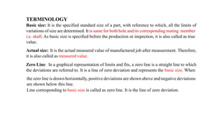
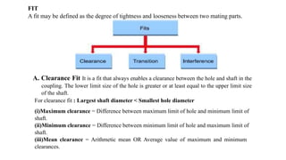
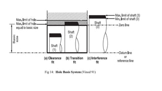
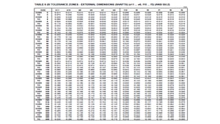
(a)Wringing fit: It provides either zero interference or a clearance. It is employed, where
parts can be replaced without difficulty during minor repairs.
(b)Push fit: It provides small clearance. It is employed for parts that must be dis-assembled
during operation of a machine. For example: Changing gears etc.
C. Interference Fit It is a fit that always ensures some interference between the hole and
shaft in the coupling. The upper limit size of the hole is smaller or at least equal to the lower
limit size of the shaft.
Therefore, for Interference fit : Smallest shaft diameter > Largest hole diameter.
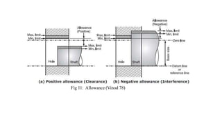
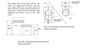
•In clearance fit, allowance is the minimum clearance, i.e. difference between minimum
size of hole and maximum size of shaft. It is referred as positive allowance. [Ref. Fig. 11(a)].
• In interference fit, allowance is the maximum interference, i.e. difference between
minimum size of hole and maximum size of shaft. It is referred as negative allowance. [Ref.
Fig. 11(b)].

(i)Maximum interference is the negative difference between the maximum limit size of the
shaft and the minimum limit size of the hole.
(ii)Minimum interference is the negative difference between minimum limit size of the shaft
and the maximum limit size of the hole.
(iii)Mean interference: Arithmetic mean or Average value of maximum and minimum
interferences.
• For example: Press fit, driving fit, shrink fit etc.
• Types: (i) Force fit, (ii) Tight fit, and (iii) Heavy force and shrink fit.
(a)Force fit: It has considerable interference between mating parts. It is employed, when
mating parts are not required to be disassembled during their total service life. Here, assembly
of mating parts is only obtained, if high pressure is applied. For example: Gears on the shaft
of concrete mixture, Forging machine etc.
(b)Tight fit: It has less interference than force fit. It is employed for the mating parts, that may
be replaced while overhauling/maintenance of the machine.
For example: Stepped pulley on the drive shaft of a conveyor, cylindrical grinding machine
etc.
(c)Heavy force and shrink fit: It has maximum interference between mating parts. Therefore,
to obtain the required fit, considerable amount of force is applied.

Maximum and Minimum Metal Conditions (MML and LML)
Let us consider a shaft having a dimension of 40 ± 0.05 mm.
For Shaft
• The maximum metal limit (MML) of the shaft will have a dimension of 40.05 mm because at this
higher limit, the shaft will have the maximum possible amount of metal.
• The shaft will have the least possible amount of metal at a lower limit of 39.95 mm, and this
limit of the shaft is known as minimum or least metal limit (LML).
• For Hole
Let us consider a hole having a dimension of ϕ 45 ± 0.05 mm.
• The hole will have a maximum possible amount of metal at a lower limit of 44.95 mm and
the lower limit of the hole is designated as MML.
• For example, when a hole is drilled in a component, minimum amount of material
is removed at the lower limit size of the hole. This lower

• The higher limit of the hole will be the
LML. At a high limit of 45.05 mm, the
hole will have the least possible amount of
metal. The maximum and minimum metal
conditions are shown in Fig. 12 (a) and
12(b)
Fig 11(a): Maximum and minimum metal
limits (anand158)
Fig 12(b): Maximum and minimum metal
limits (anand158)

Tolerances Grades and Fundamental Deviation(Anand 166)
The tolerance of a size is defined as the difference between the upper and lower limit
dimensions of the part.
In order to meet the requirements of various production methods for accuracy of the product,
the IS: 919 system, implements 18 grades of accuracy (tolerances). Each of the tolerances of
this system is marked IT with the attached grade of accuracy (IT01, IT0, IT1 ... IT16). But,
ISO: 286: 1988 specifies 20 grades of tolerances (i.e., from IT01 to IT18)

Ref. Size and Tolerance (Dr Ala Hizazi)

Tolerance symbols: These are used to specify the tolerance and fits for mating components.
For example, in 40 H8f7, the number 40 indicates the basic size in millimeters; capital letter
H (Class of Tolerance) indicates the fundamental deviation for the hole; and lower‐case
letter f indicates the shaft. The numbers following the letters indicate corresponding IT
grades.
Fig 13: fundamental deviation and tolerance zone w.r.t the zero line (Anand 168)

Hole Basis System (Vinod 85)
•In this system, the design size of hole, whose lower deviation (fundamental deviation) is zero,
is assumed as basic size and different clearances or interferences are obtained by varying the
limits of mating part i.e. shaft to have different class of fit.
•In other words, limits of hole are kept constant and limits of shaft are varied, so as to obtain
the necessary type of fit.
Advantages of Hole Basis System:
(i)As hole basis system is very easy, convenient and less costly to make holes of correct sizes
by using drills, reamers etc., therefore, hole basis system is preferred and used by almost all
industrial companies.
(ii)It is also much easier to vary shaft sizes according to the fit required, by suitable methods
such as turning and grinding.
(iii)Also, inspection of shafts can be done easily and rapidly with the help of adjustable
gauges. Direct external measurement (such as shaft) is easier than internal measurement (such
as hole).

Fig 14: Hole Basis System (Vinod 91)

Shaft Basis System
•In this system, the design size of a shaft, whose upper deviation (fundamental deviation) is
zero, is assumed as basic size and different clearances or interferences are obtained by varying
the limits of hole to have different types of fit.
•In other words, limits of shaft are kept constant and limits of holes are varied to obtain the
necessary type of fit.
Advantage of Shaft Basis System:
(i) It is preferred, when different accessories with different fits such as pulley, bearings, gears
etc. are mounted on a single large shaft.
Fig 15: Shaft Basis System (Vinod 86)

Designation of Holes and Shafts
1) Hole = 55 H7 means
55 = the basic size of the hole
H = the position of the hole w.r.t zero line. For this case it is on the zero line.
7 = the tolerance grade, i.e., IT7. By knowing this value, the limits for 55-mm
size can be found out.
2) Shaft = 60 m9 means
60 = the basic size of the shaft.
m = the position of the shaft w.r.t zero line. In this case, it is above the zero line.
9 = the tolerance grade, i.e., IT9. By knowing this value, the limits for 60-mm size can
be found out.

Hole ‘A’ and shaft ‘a’ have the largest fundamental deviations, hole being positive
and shaft being negative. The fundamental deviations for both hole ‘H’ and shaft
‘h’ are zero. For the shafts ‘a’ to ‘g’, the upper deviation is below the zero line,
and for the shafts ‘j’ to ‘zc’, it is above the zero line.
For the holes ‘A’ to ‘G’, the lower deviation is above the zero line, and for the holes
‘J’ to ‘Zc’; it is below the
zero line. The shaft for which upper deviation is zero is called basic shaft (i.e., ‘h’)
and the hole for which lower deviation is zero is called basic hole (i.e., ‘H’)

Fig 17: Position of fundamental
deviations

The Upper and Lower deviations for Hole are donated by "ES" and "EI"
ES=EI+IT, and for shaft es=ei+IT
The calculation for tolerance grade is done as follows:
The fundamental tolerance unit is denoted as i (in microns). It is used to express various IT
grades from IT5 to IT16, where the value of i in terms of the diameter D (in mm) can be
calculated as
i = 0.45 3
√𝐷 + 0.001D
The diameter ‘D’ (in mm) is the geometric mean of the diameter steps (please refer Table 2.1).
Tolerances are same for all diameter sizes, which fall in the specific range of the diameter
step.
Table 2.1 Geometric mean of diameter steps

The values of tolerances for tolerance grades IT5 to IT16 are given in Table 2.2.
For the values of tolerance grades IT01 to IT4, the formulae are
For IT01 = 0.3 + 0.008D
For IT0 = 0.5 + 0.012D
For IT1 = 0.8 + 0.02D
Table 2.2 Tolerance grades IT5 to IT16

Illustration for Determining Type of Fit
Determine type of Fit of 55 H7 f8:
1. Determine value of D = 50×65 = 57.008 mm
2. Determine value of i = 0 45× 3
√57 008 3 + 0.001 (57.008) = 1.789 microns.
3. Now consider first for Hole H7,
Value for the Tolerance IT7 (From Table 2.2) = 16 (i ) = 16 (1.789) = 0.028 mm
As the H-hole lies on the zero line (refer Fig. 17), its fundamental deviation is zero and lower
deviation is zero.
Basic size = 55 mm
∴ Basic size + Fundamental deviation = Lower limit of size = 55 mm
∴ Lower limit + Tolerance = Upper limit
i.e., 55 mm + 0.028 = 55.028 mm
Hence, hole size varies between 55.00 mm to 55.028 mm.

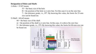
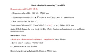
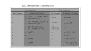
4. Now consider for shaft 55f8,
Value for the tolerance IT8 (From Table 2.2) = 25 (i ) = 25 (1.789 microns) = 0.0447 mm
As the f-shaft lies below the zero line (refer Fig. 17), its fundamental deviation is the upper deviation.
Hence, the formula for fundamental deviation from Table 2.3 is = [−5.5 D 0 . 41 ].
−5.5 D 0 . 41 = = −5.5 (57.0.08) 0 . 41 = = −28.86 microns = −0.0288 mm
∴ Now, upper limit of shaft = Basic size + Fundamental deviation
= 55 mm + (−0.0288) = 54.9712 mm
And, lower limit of shaft = Upper limit of shaft + Value for the Tolerance IT8
= 54.9712 − 0.0447 = 54.9265 mm
Hence, shaft size varies between 54.9712 mm to 54.9265 mm. and hole size varies
between 55.00 mm to 55.028 mm.
5. To check the type of fit we have to calculate
Maximum clearance = 55.028 mm − 54.9265 mm = 0.1015 mm [∴ clearance exists] Minimum
clearance = 55.00 mm -54.9712 mm = 0.028 mm [∴ clearance exists]
6.Therefore, we can conclude that the type of fit of 55 H7f8 assembly results into ‘Clearance fit’.

Table 2.3 Fundamental deviations for shaft

Design of Gauges
30 H6d8
H6. Tolerance
0.013 mm(table 6.10 Tolerance table)
−.065
d8 Tolerance 30−.098 = 0.033( table 6.19)

Module 2 part i limits, fits, and tolerances

Module 2 part i limits, fits, and tolerances

Recommended

Recommended

More Related Content

What's hot

What's hot (20)

Similar to Module 2 part i limits, fits, and tolerances

Similar to Module 2 part i limits, fits, and tolerances (20)

Recently uploaded

Recently uploaded (20)

Module 2 part i limits, fits, and tolerances