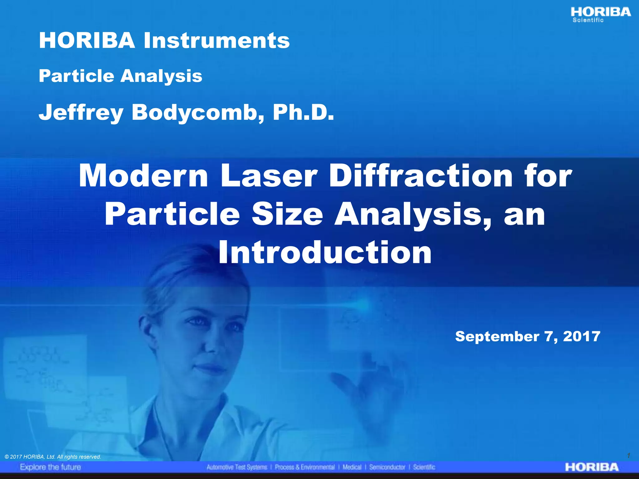
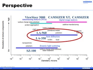
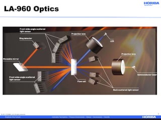
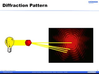
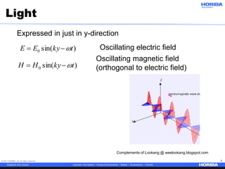
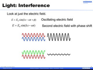
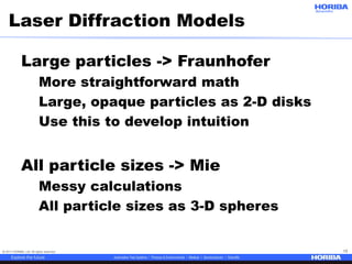
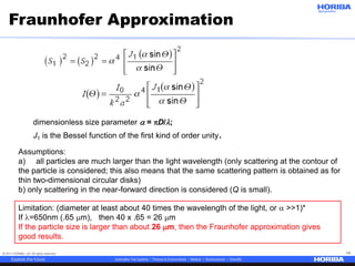
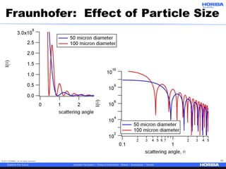
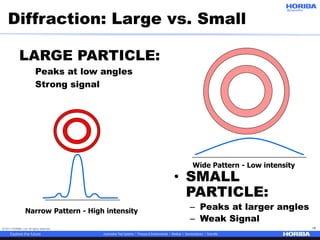
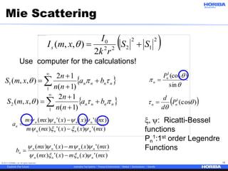
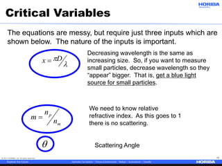
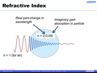
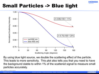
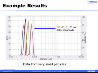
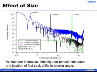
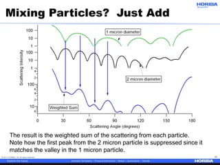
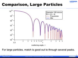
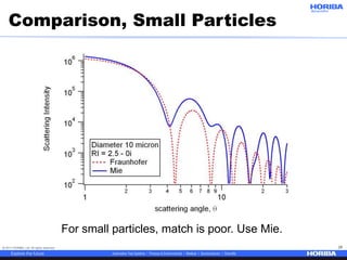
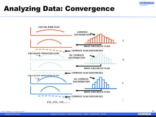
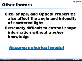
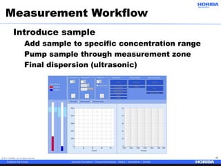
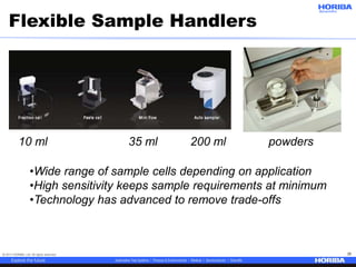
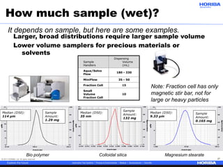
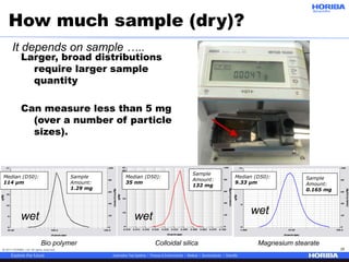
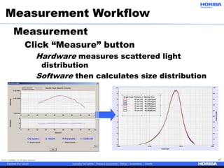
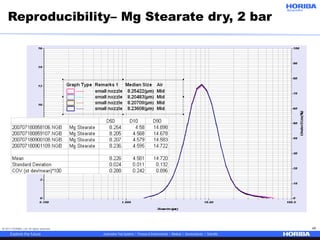
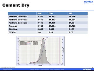
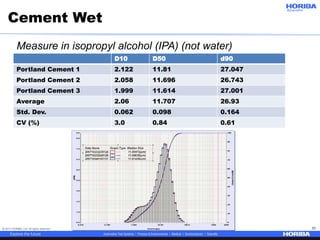
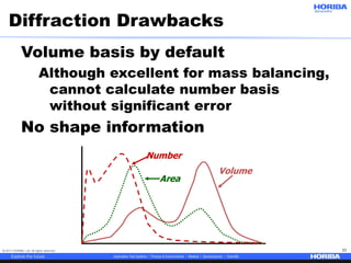
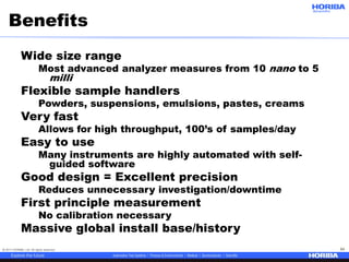
Modern Laser Diffraction for Particle Analysis

© 2017 HORIBA, Ltd. All rights reserved. 1© 2017 HORIBA, Ltd. All rights reserved. 1
Modern Laser Diffraction for
Particle Size Analysis, an
Introduction
Particle Analysis
Jeffrey Bodycomb, Ph.D.
September 7, 2017
HORIBA Instruments

© 2017 HORIBA, Ltd. All rights reserved. 2
Perspective
SZ-100
LA-960
LA-350
ViewSizer 3000 CAMSIZER XT, CAMSIZER

Why Particle Size?
Industry Industry
Ceramic Construction
Oil/rubber Chemical
Battery Pharmaceutical
Electricity Food/Drink
Automobile Paper/Pulp
Mining Ink/Toner
Size affects material behavior and processing across a
number of industries.

Application: Pigment Hiding Power
Operator dependent, need to
wait for drying.
Operator independent, no need
to wait for drying.

Core Principle
Investigate a particle with light and
determine its size

When a Light beam Strikes a Particle
Some of the light is:
Diffracted
Reflected
Refracted
Absorbed and Reradiated
• Small particles require knowledge of optical properties:
– Real Refractive Index (bending of light, wavelength of
light in particle)
– Imaginary Refractive Index (absorption of light within
particle)
– Refractive index values less significant for large
particles
• Light must be collected over large range of angles
Reflected
Refracted
Absorbed
and
Reradiated
Diffracted

LA-960 Optics

Diffraction Pattern

Light
)sin(0 tkyHH 
)sin(0 tkyEE  Oscillating electric field
Oscillating magnetic field
(orthogonal to electric field)
Expressed in just in y-direction
Complements of Lookang @ weelookang.blogspot.com

Light: Interference
)sin(0   tkxEE
)sin(0 tkxEE 
Oscillating electric field
Look at just the electric field.
Second electric field with phase shift


Path length difference is s sin(
s
Detector (far
away)
r0
Path Length Difference

Scattering data typically cannot be
inverted to find particle shape.
We use optical models to interpret
data and understand our
experiments.
Use models to interpret data

Large particles -> Fraunhofer
More straightforward math
Large, opaque particles as 2-D disks
Use this to develop intuition
All particle sizes -> Mie
Messy calculations
All particle sizes as 3-D spheres
Laser Diffraction Models

Fraunhofer Approximation
dimensionless size parameter a = pD/l;
J1 is the Bessel function of the first kind of order unity.
Assumptions:
a) all particles are much larger than the light wavelength (only scattering at the contour of
the particle is considered; this also means that the same scattering pattern is obtained as for
thin two-dimensional circular disks)
b) only scattering in the near-forward direction is considered (Q is small).
Limitation: (diameter at least about 40 times the wavelength of the light, or a >>1)*
If l=650nm (.65 mm), then 40 x .65 = 26 mm
If the particle size is larger than about 26 mm, then the Fraunhofer approximation gives
good results.

Fraunhofer: Effect of Particle Size

LARGE PARTICLE:
Peaks at low angles
Strong signal
• SMALL
PARTICLE:
– Peaks at larger angles
– Weak Signal
Wide Pattern - Low intensity
Narrow Pattern - High intensity
Diffraction: Large vs. Small

Poll
How many of you work with
particles with sizes over 1 mm?
particles with sizes over 25
microns?
particles with sizes less than 1
micron?

Mie Scattering
 nnnn ba
nn
n
xmS p 


 

1
2
)1(
12
),,(
 2
1
2
222
0
2
),,( SS
rk
I
xmIs 
)(')()(')(
)(')()(')(
mxxxmxm
mxxxmxm
a
nnnn
nnnn
n





 nnnn ba
nn
n
xmS p 


 

1
1
)1(
12
),,(
)(')()(')(
)(')()(')(
mxxmxmx
mxxmxmx
b
nnnn
nnnn
n





, : Ricatti-Bessel
functions
Pn
1:1st order Legendre
Functions


p
sin
)(cos1
n
n
P

 )(cos1


 nn P
d
d

Use computer for the calculations!

Critical Variables

l
pDx 
m
p
n
n
m 
Decreasing wavelength is the same as
increasing size. So, if you want to measure
small particles, decrease wavelength so they
“appear” bigger. That is, get a blue light
source for small particles.
The equations are messy, but require just three inputs which are
shown below. The nature of the inputs is important.
We need to know relative
refractive index. As this goes to 1
there is no scattering.
Scattering Angle

Refractive Index
n = 1 (for air)
n = 2-0.05i
Real part-change in
wavelength
Imaginary part-
absorption in particle

By using blue light source, we double the scattering effect of the particle.
This leads to more sensitivity. This plot also tells you that you need to have
the background stable to within 1% of the scattered signal to measure small
particles accurately.
Small Particles -> Blue light

30, 40, 50, 70 nm
latex standards
Data from very small particles.
Example Results

Effect of Size
As diameter increases, intensity (per particle) increases
and location of first peak shifts to smaller angle.

Mixing Particles? Just Add
The result is the weighted sum of the scattering from each particle.
Note how the first peak from the 2 micron particle is suppressed since it
matches the valley in the 1 micron particle.

Comparison, Large Particles
For large particles, match is good out to through several peaks.

Comparison, Small Particles
For small particles, match is poor. Use Mie.

Glass Beads and Models

CMP Slurry

Analyzing Data: Convergence

Other factors
Size, Shape, and Optical Properties
also affect the angle and intensity
of scattered light
Extremely difficult to extract shape
information without a priori
knowledge
Assume spherical model

Pop Quiz
What particle shape is used for
laser diffraction calculations?
A. Hard sphere
B. Cube
C. Triangle
D. Easy sphere

Pop Quiz
What particle shape is used for
laser diffraction calculations?
A. Hard sphere
B. Cube
C. Triangle
D. Easy sphere
Either gets full credit!

Measurement Workflow
Prepare the sample
Good sampling and dispersion a must!
May need to use surfactant or
admixture

Prepare the system
Align laser to maximize signal-to-noise
Acquire blank/background to reduce
noise

Introduce sample
Add sample to specific concentration range
Pump sample through measurement zone
Final dispersion (ultrasonic)

10 ml 35 ml 200 ml powders
•Wide range of sample cells depending on application
•High sensitivity keeps sample requirements at minimum
•Technology has advanced to remove trade-offs
Flexible Sample Handlers

How much sample (wet)?
Larger, broad distributions require larger sample volume
Lower volume samplers for precious materials or
solvents
Sample
Handlers
Dispersing
Volume
(mL)
Aqua/Solvo
Flow
180 - 330
MiniFlow 35 - 50
Fraction Cell 15
Small
Volume
Fraction Cell
10
Median (D50):
35 nm
Sample
Amount:
132 mg
Median (D50):
114 µm
Sample
Amount:
1.29 mg
Median (D50):
9.33 µm
Sample
Amount:
0.165 mg
Note: Fraction cell has only
magnetic stir bar, not for
large or heavy particles
Bio polymer Colloidal silica Magnesium stearate
It depends on sample, but here are some examples.

How much sample (dry)?
Larger, broad distributions
require larger sample
quantity
Can measure less than 5 mg
(over a number of particle
sizes).
Median (D50):
35 nm
Sample
Amount:
132 mg
Median (D50):
114 µm
Sample
Amount:
1.29 mg
Median (D50):
9.33 µm
Sample
Amount:
0.165 mg
Bio polymer Colloidal silica Magnesium stearate
It depends on sample …..
wet wet
wet

Method Workflow
First determine RI
Choose solvent (water, surfactants,
hexane, etc.)
Sampler selection: sample volume
Pump & stirrer settings
Concentration
Measurement duration
Does the sample need ultrasound?
Document size-time plot
Disperse sample, but don’t break particles
Check for reproducibility

Determine Refractive Index
Real component via literature or web search, Becke line, etc.
Measure sample, vary imaginary component to see if/how
results change
Recalculate using different imaginary components, choose
value that minimizes R parameter error calculation

Concentration
High enough for good S/N ratio
Low enough to avoid multiple
scattering
Typically 95 – 80 %T
Measure at different T%, look at
d50 result, Chi Square
calculation
d50
Chi2

Ultrasonic Dispersion
Adding energy to break up agglomerates – disperse to
primary particles, without breaking particles
Similar to changing air pressure on dry powder feeder
Typically set to 100% energy, vary time (sec) on
Investigate tails of distribution
High end to see if agglomerates removed
Small end to see if new, smaller particles appear (breakage)
Test reproducibility, consider robustness
Note:
Do not use on emulsions
Can cause thermal mixing trouble w/solvents - wait
Use external probe if t> 2-5 minutes

Size
Increasing energy
Stability
Theoretical Actual
Size
Increasing energy
Higher air pressure or longer ultrasound duration
Dispersion vs. Breakage

Dispersion vs. Breakage
Dispersion and milling can be parallel
rather than sequential processes
Theoretical
Actual

Effect of Air Pressure: MCC

LA-960 Method Expert
Method Expert guides user to prepare
the LA-960 for each test
Results displayed in multiple formats:
PSD, D50, R-parameter

Measurement
Click “Measure” button
Hardware measures scattered light
distribution
Software then calculates size distribution

Reproducibility– Mg Stearate dry, 2 bar

Cement Dry
D10 D50 d90
Portland Cement 1 3.255 11.152 24.586
Portland Cement 2 3.116 11.183 24.671
Portland Cement 3 3.112 11.128 24.92
Average 3.161 11.154 24.726
Std. Dev. 0.082 0.027 0.173
CV (%) 2.6 0.24 0.70

Cement Wet
D10 D50 d90
Portland Cement 1 2.122 11.81 27.047
Portland Cement 2 2.058 11.696 26.743
Portland Cement 3 1.999 11.614 27.001
Average 2.06 11.707 26.93
Std. Dev. 0.062 0.098 0.164
CV (%) 3.0 0.84 0.61
Measure in isopropyl alcohol (IPA) (not water)

Instrument to instrument variation
Sample CV D10 CV D50 CV D90
PS202 (3-30µm) 2% 1% 2%
PS213 (10-100µm) 2% 2% 2%
PS225 (50-350µm) 1% 1% 1%
PS235 (150-650µm) 1% 1% 2%
PS240 (500-2000µm) 3% 2% 2%
These are results from running polydisperse
standards on 20 different instruments
20 instruments, 5 standards

Instrument to instrument variation
Industrial Samples
4 instruments, real sample

Diffraction Drawbacks
Volume basis by default
Although excellent for mass balancing,
cannot calculate number basis
without significant error
No shape information
Volume
Area
Number

Benefits
Wide size range
Most advanced analyzer measures from 10 nano to 5
milli
Flexible sample handlers
Powders, suspensions, emulsions, pastes, creams
Very fast
Allows for high throughput, 100’s of samples/day
Easy to use
Many instruments are highly automated with self-
guided software
Good design = Excellent precision
Reduces unnecessary investigation/downtime
First principle measurement
No calibration necessary
Massive global install base/history

Q&A
Ask a question at labinfo@horiba.com
Keep reading the monthly HORIBA Particle
e-mail newsletter!
Visit the Download Center to find the video
and slides from this webinar.
www.horiba.com/us/particle
Jeff Bodycomb, Ph.D.
P: 866-562-4698
E: jeff.bodycomb@horiba.com

Modern Laser Diffraction for Particle Analysis

More Related Content

What's hot

Similar to Modern Laser Diffraction for Particle Analysis

More from HORIBA Particle

Recently uploaded

Modern Laser Diffraction for Particle Analysis