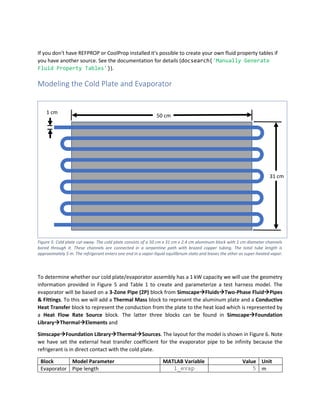
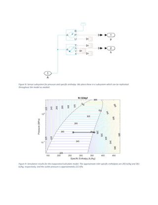
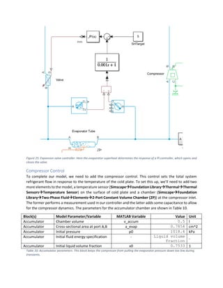
This document provides a tutorial on modeling a closed-loop refrigeration system using Simscape Fluids, specifically designed to maintain a 10 kg aluminum cold plate at 5°C while handling a 1 kW heat load. The system consists of four main components: an evaporator, a condenser, a compressor, and an expansion valve, all configured with specific parameters and control systems aimed at optimizing performance under varying environmental temperatures. The tutorial also covers the selection of working fluid properties, initial boundary conditions, and steps to visualize and validate the system's performance through simulations.
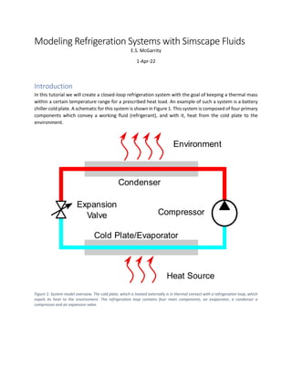
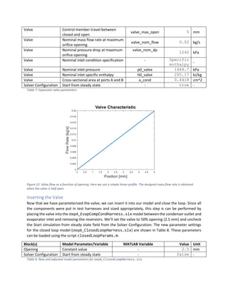
![Figure 3: Two-Phase Fluid Predefined Properties block (left) and dialog (right). Here we select R-1234yf to automatically define
the fluid property tables.
Alternately, if we have access to REFPROP (1) or CoolProp (2) software, we can use the
twoPhaseFluidTables() function to retrieve the properties as a struct in MATLAB and push this into
the Two-Phase Fluid Properties block. This block can be found in Simscape→Foundation Library→Two-
Phase Fluid→Utilities→Two-Phase Fluid Properties (2P). To get started, place this block into an empty
Simscape model, and name it R1234yf. Save your Simulink model as FluidProps.slx. Next, retrieve
the properties from the fluid database with the command1
:
R1234yf_Props = ...
twoPhaseFluidTables([140,450],[0,1.3],25,25,60,'R1234yf',...
'C:Program Files (x86)REFPROP10');
This will create a variable in the MATLAB workspace with the required properties. Finally, push the
properties into the fluid properties block with a second execution of the command:
twoPhaseFluidTables('FluidProps/R1234yf', R1234yf_Props);
The resulting Parameters tab in the Two-Phase Fluid Properties block will appear as shown in Figure 4.
Figure 4: Fluid properties dialog for the R-1234yf working fluid.
1
The final argument to the twoPhaseFluidTables() command is the path to your REFPROP or CoolProp
installation. This will vary from computer to computer.](https://image.slidesharecdn.com/modelingrefrigerationsystemsinsimscape-240921174317-66c7a94f/85/Modeling-Refrigeration-Systems-in-Simscape-pdf-4-320.jpg)
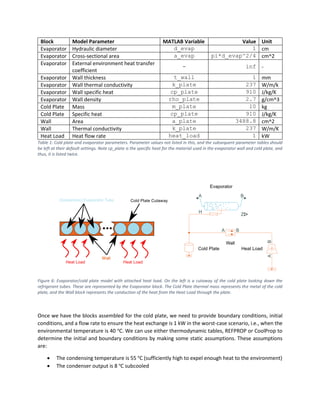
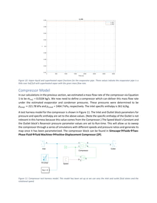
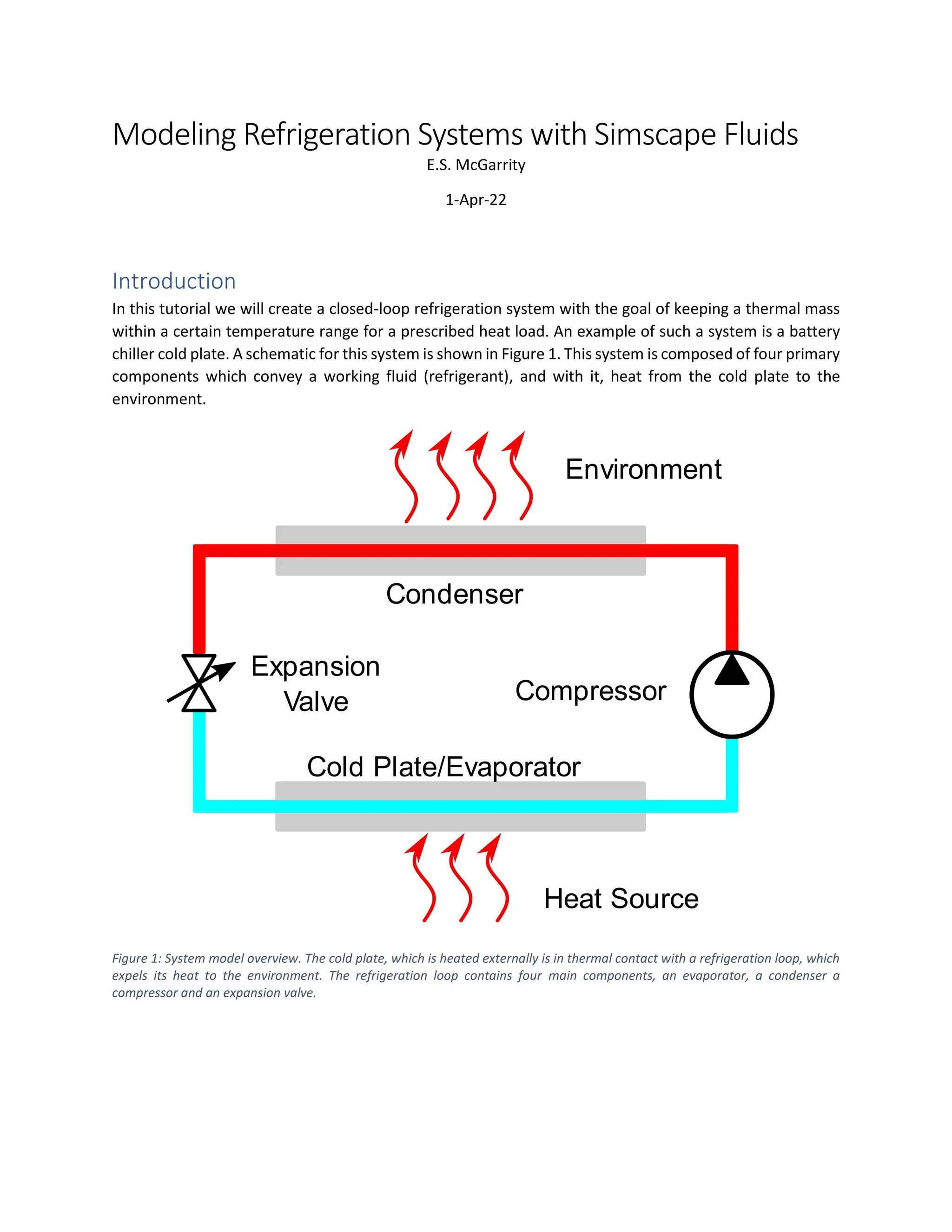
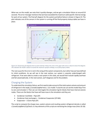
![The model for the complete compressor test harness can be found in step2_CompressorHarness.slx
and its parameters can be loaded with the compressorParams.m routine. The parameters are
summarized in Table 3. At these settings, the compressor adds about 0.5 kW of heat to the fluid.
Block(s) Model Parameter/Variable MATLAB Variable Value Unit
Inlet Reservoir pressure p1_comp 221.78 kPa
Inlet Reservoir specific enthalpy h1_comp 265.17 kJ/kg
Outlet Reservoir pressure p2_comp 1464.7 kPa
Compressor Nominal mass flow rate mdot_comp 0.0104 kg/s
Compressor Nominal shaft speed N_comp 3600 rpm
Compressor Nominal inlet pressure p_nom_in 221 kPa
Compressor Nominal inlet temperature T_nom_in 278.15 K
Compressor Nominal volumetric efficiency eta_v 0.95 -
Compressor Nominal pressure ratio pr_nom 6 -
Compressor Polytropic exponent gamma1234yf 1.14 -
Compressor Mechanical efficiency eta_m 0.9 -
Compressor
Speed Constant N_0 3600 rpm
Solver Configuration Start from steady state - true(checked) -
Table 3: Compressor model parameters.
Compressor Map
To see what the compressor map looks like based on the given parameters, we can write a script to
exercise the harness model we created across a range of shaft speeds and pressure ratios. The code for
performing this parameter sweep is given in the file compressorSweep.m. We will analyze the relevant
parts of this script in this section.
To begin, we open the model and set up its parameters in the MATLAB workspace. This is on lines 1-8:
% Build compressor map
% Open the model in case it is not.
mdl = 'CompressorHarness';
open_system(mdl);
% Load the parameters
compressorParams;
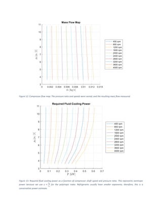
Next, we set up the design of experiments (DOE) for the parameter sweep. The goal is to sweep the
compressor speed from 400 to 4000 rpm and the outlet pressure from 800 to 2400 kPa. This will exercise
the compressor across pressure ratios from about 3 to 11, which should provide a reasonable map for the
expected operating conditions. The key lines for setting up the DOE are 12-13 and 21:
N_lis = 0:400:4000; % [rpm]
p2_lis = 800:400:2400; % [kPa]
[N_mat, p2_mat] = ndgrid(N_lis, p2_lis);](https://image.slidesharecdn.com/modelingrefrigerationsystemsinsimscape-240921174317-66c7a94f/85/Modeling-Refrigeration-Systems-in-Simscape-pdf-11-320.jpg)
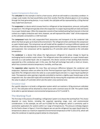
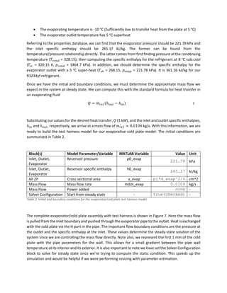
![Once the DOE is formulated, we can create a Simulink.SimulationInput object, which will be used
to set the parameters of the model during a sequence of Simulink runs. This is done on lines 24-32 of the
script:
simin(1:N_sim) = Simulink.SimulationInput(mdl);
% Setup the parameters used by the model
for k = 1:N_sim
simin(k) = simin(k).setBlockParameter([mdl '/Speed'], ...
'constant', num2str(N_mat(k)));
simin(k) = simin(k).setBlockParameter([mdl '/Outlet'], ...
'reservoir_pressure', num2str(p2_mat(k)));
end
With the simulation inputs defined, we can now execute them. This happens on line 36:
simout = sim(simin, 'ShowSimulationManager', 'off', 'UseFastRestart', 'on');
The code sweeps across 10 speeds and 5 pressure ratios for a total of 50 simulations. These simulations
can be performed in under a minute on a modest workstation with Simulink’s Fast Restart capability. Once
the code is finished with the sweep, we can extract the parameters and plot them. The code for parameter
extraction is on lines 39-47:
mdot = N_mat*0;
fp = mdot;
for k = 1:N_sim
% Get the last elements of the mass flow and fluid power vars
mlog = simout(k).simlog.Compressor.mdot_A.series.values('kg/s');
mdot(k) = mlog(end);
fplog = simout(k).simlog.Compressor.fluid_power.series.values('kW');
fp(k) = fplog(end);
end
Note the destination arrays (mdot and fp) have been allocated to be the same shape as the input grids.
This will allow us to easily extract the speed lines for the sweeps when we plot the data. The plotting code
is on lines 50-74. The resulting plots can be seen in Figure 12 and Figure 13.](https://image.slidesharecdn.com/modelingrefrigerationsystemsinsimscape-240921174317-66c7a94f/85/Modeling-Refrigeration-Systems-in-Simscape-pdf-12-320.jpg)
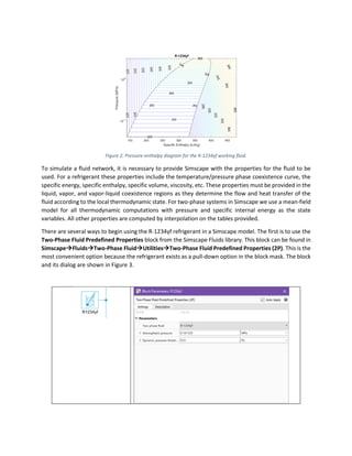
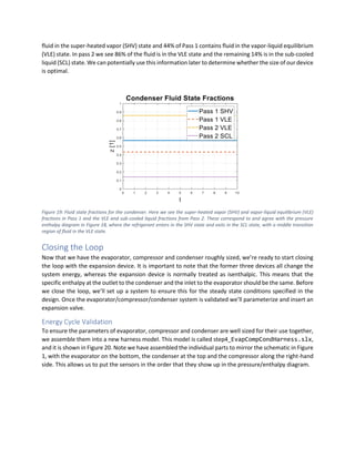
![𝑙𝑓𝑖𝑛 = 𝑁𝑡𝑝𝑟 ⋅ (𝑤𝑡𝑢𝑏𝑒 + 𝑡𝑤𝑎𝑙𝑙) + 𝑡𝑤𝑎𝑙𝑙,
where 𝑤𝑡𝑢𝑏𝑒 is the tube width (2 mm), and 𝑁𝑡𝑝𝑟 is the number of tubes per row in the condenser. The
fins span the gaps between the tube banks perpendicular to the airflow and, therefore, have widths of
𝑤𝑓𝑖𝑛 = ℎ𝑐𝑜𝑛𝑑 − 𝑁𝑟𝑜𝑤 ⋅ (ℎ𝑡𝑢𝑏𝑒 + 2 ⋅ 𝑡𝑤𝑎𝑙𝑙),
where ℎ𝑐𝑜𝑛𝑑 is the condenser height, 𝑁𝑟𝑜𝑤 is the total number of tube banks, and ℎ𝑡𝑢𝑏𝑒 is the tube height
(1 mm). This along with the fin length gives the fin area to be approximately
𝑎𝑓𝑖𝑛 = 𝑙𝑓𝑖𝑛 ⋅ 𝑤𝑓𝑖𝑛.
Here we assume the fins are independent of each other and aligned vertically with a density of 5 fins per
cm (𝜌𝑓𝑖𝑛), which is a reasonable approximation for this type of condenser hardware. With this assumption,
we calculate the total fin area, 𝑎𝑓𝑖𝑛𝑡𝑜𝑡, to be
𝑎𝑓𝑖𝑛𝑡𝑜𝑡 = 𝑁𝑟𝑜𝑤 ⋅ 𝑎𝑓𝑖𝑛 ⋅ 𝜌𝑓𝑖𝑛 ⋅ 𝑙𝑡𝑢𝑏𝑒,
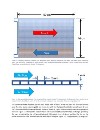
where 𝑙𝑡𝑢𝑏𝑒 is the tube length, which is equal to the condenser width minus the side manifold widths (1
cm each).
The entrance and exits of the condenser and the connection between its two passes are represented as
pipes. These pipes are not thermally connected, but serve to add capacitance to the condenser, which is
key to preventing the tubes from flooding during high temperature operations once the condenser is
placed into the closed-loop system.
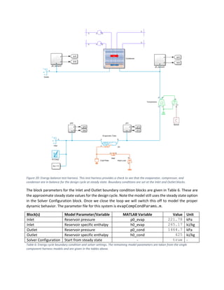
The condenser model can be found in Condenser_2Pass.slx. This model is located in a Subsystem
Reference, which we can instantiate inside the test harness (step3_CondenserHarness.slx) to
evaluate its performance. Later we will use this same Subsystem Reference in the complete model. This
is good practice because we will be able to reuse the same condenser model inside other models and
ensure changes to the test harness model are reflected in the main model. Note that in this case, we have
promoted only the parameters we will need for our exercises, i.e., the initial pressure and energy settings
for the manifolds and heat exchangers. The layout of the condenser is shown in Figure 17. It uses two
Condenser-Evaporator (2P-MA) blocks, one for each of the two passes, and three pipe blocks to represent
the manifolds. These blocks can be found in the libraries under Simscape→Fluids→Fluid Network
Interfaces→Heat Exchangers→Condenser-Evaporator (2P-MA) and Simscape→Foundation
Library→Two-Phase Fluid→Elements→Pipe (2P).
The initialization of the fin area plus the other parameters for the condenser unit are performed in the
condenserParams.m MATLAB script. This script handles the air-side and refrigerant-side parameters as
well as the initial conditions for the model step3_CondenserHarness.slx. The parameters for the
condenser harness are shown in Table 4. The condenser model parameters are given in Table 5.
Block(s) Model Parameter/Variable MATLAB Variable Value Unit
Inlet, Outlet Reservoir pressure p0_cond 1464.7 kPa
Inlet Reservoir specific enthalpy h0_cond 425 kJ/kg
Ref Flow Mass flow rate mdot_cond 0.0104 kg/s
Air In1, Air In2 Temperature T_air_cond 40 degC
Air Flow(1,2) Mixture mass flow rate mdot_air_cond(1,2) [0.15, 0.05] kg/s](https://image.slidesharecdn.com/modelingrefrigerationsystemsinsimscape-240921174317-66c7a94f/85/Modeling-Refrigeration-Systems-in-Simscape-pdf-16-320.jpg)
![Table 4:Condenser test harness parameters. The air flow and environment temperature are set to the
worst-case scenario outlined above.
Figure 17: Simscape layout for the 2-pass condenser. The refrigerant passes are in series and the air passes are in parallel.
Block(s) Model Parameter/Variable MATLAB Variable Value Unit
Pass(1,2) Flow arrangement - Crossflow -
Pass(1,2) Cross-sectional area A1,B1 a_cond 0.4418 cm^2
Pass(1,2) Cross-sectional area A2,B2 a_x_cond(1,2) [1800, 600] cm^2
Pass(1,2) TPF: Number of tubes N_tube_pass(1,2) [240 80] -
Pass(1,2) TPF: Total length of each tube l_tube 56 cm
Pass(1,2) TPF: Tube cross section - Rectangular -
Pass(1,2) TPF: Tube width w_tube 2 mm
Pass(1,2) TPF: Tube height h_tube 1 mm
Pass(1,2) TPF: Initial fluid energy
specification
- Specific
enthalpy -
Pass(1,2) TPF: Initial two-phase fluid
pressure
p0_cond
1464.7 kPa
Pass(1,2) TPF: Initial two-phase fluid specific
enthalpy
h0_cond
425 kJ/kg
Pass(1,2) MA: Flow geometry - Generic -
Pass(1,2) MA: Minimum free-flow area a_maflow(1,2) [913.5
304.5] cm^2](https://image.slidesharecdn.com/modelingrefrigerationsystemsinsimscape-240921174317-66c7a94f/85/Modeling-Refrigeration-Systems-in-Simscape-pdf-17-320.jpg)
![Block(s) Model Parameter/Variable MATLAB Variable Value Unit
Pass(1,2) MA: Heat transfer surface area
without fins
a_x_httubes(1,2)
[4611 1537] cm^2
Pass(1,2) MA: Moist air volume inside heat
exchanger
v_ma(1,2) [1872.7
624.23] cm^2
Pass(1,2) MA: Coefficients [a,b,c] for
a*Re^b*Pr^c
REPRabc
[0.12 1 0.4] -
Pass(1,2) MA: Total fin surface area a_fins(1,2) [1.4268
0.4756] m^2
Pass(1,2) MA: Initial moist air temperature T_air_cond 40 degC
Manifold(1,2,3) Pipe length lman(1,2,3) [30 40 10] cm
Manifold(1,2,3) Cross-sectional area a_man 5 cm^2
Manifold(1,2,3) Hydraulic diameter d_man 2.222 cm
Solver Configuration Start from steady state - true -
Table 5: Model parameters for the 2-pass condenser. The numbers in parentheses indicate block identities or array elements. For
example, Pass 1 uses a_x_cond(1) for its Cross-sectional areas A2 and B2 and Pass 2 uses a_x_cond(2). For cases where the
MATLAB variable is a scalar, all elements use the same value, e.g., Pass 1 and Pass 2 both use a_cond for their refrigerant port
areas A1, and B1.
To validate the condenser model for the above parameters, we can examine the pressure-enthalpy
diagram in Figure 18. Under the given conditions, the fluid state starts on the right end of the segment as
a super-heated vapor and ends on the left end of the segment as sub-cooled liquid.
Figure 18: Condenser pressure/enthalpy diagram at steady state for the design case scenario. Fluid enters the condenser in the
state indicated by the circle on the right end of the line segment (as super-heated vapor) and leaves at the state indicated by
the circle on the left end of the segment (sub-cooled liquid).
As the fluid moves through the first pass of the condenser tubes, it begins to condense and enters the
vapor-liquid equilibrium dome. In the second pass, the fluid crosses the saturated liquid boundary and
leaves as a sub-cooled liquid. To ensure the latter is true, we plot selected state fractions of the fluids in
the condenser passes in Figure 19. From this figure we can see about 56% of the length of Pass 1 contains](https://image.slidesharecdn.com/modelingrefrigerationsystemsinsimscape-240921174317-66c7a94f/85/Modeling-Refrigeration-Systems-in-Simscape-pdf-18-320.jpg)
![% Condenser masses for manifolds and heat exchanger blocks
mm1 = out.simlog.Condenser.Manifold_1.mass.series.values('kg');
mm2 = out.simlog.Condenser.Manifold_2.mass.series.values('kg');
mm3 = out.simlog.Condenser.Manifold_3.mass.series.values('kg');
mp1 = out.simlog.Condenser.Pass_1.two_phase_fluid.mass.series.values('kg');
mp2 = out.simlog.Condenser.Pass_2.two_phase_fluid.mass.series.values('kg');
% Evaporator tube mass
me = out.simlog.Evaporator_Tube.mass.series.values('kg');
The total mass of the system can be computed by summing these variables as on line 21. The remainder
of the script computes the volume of the above blocks and the total system density. For the system as it
is currently parameterized, we arrive at a total mass of 0.648 kg, volume of 0.00115 m^3 and density of
56.3 kg/m^3. A realistic value for the charge density in a R1234yf refrigerant system is about 200-300
kg/m^3, so we can conclude our system is undercharged2
.
To compute the correct system density for the system at rest in some ambient condition, we need to
consult the property tables for the fluid. In our case, we’ll start our system out in the worst-case
environment at T=40 o
C. The pressure of R1234yf under this condition can be found from a
pressure/temperature table at vapor-liquid phase coexistence to be 1018.4 kPa. This gives us the initial
pressure condition for the pipes and heat exchangers.
Before we compute the system density, we must first observe that to be effective, when the system is at
rest the refrigerant must be in vapor-liquid coexistence in all its elements. Being completely liquid or
completely vapor would not allow the fluid to undergo sufficient phase transition (either because it can’t
vaporize or because it can’t form enough liquid) to perform its cooling task. With this in mind, we will
specify the initial vapor quality in the pipes and heat exchangers.
To compute the initial system quality, we can query a thermal properties database (e.g., REFPROP) as we
demonstrated earlier, with temperature T=40 o
C and density=200 kg/m^3. Alternately, we can get the
vapor and liquid densities at the given temperature and interpolate. For R1234yf at 40 o
C we have a liquid
density of 𝜌𝑙=1034 kg/m^3 and a vapor density of 𝜌𝑣=57.75 kg/m^3. To compute the vapor quality
required to achieve our target density of 𝜌𝑟𝑒𝑓=200 kg/m we can use the following equation
𝜌𝑟𝑒𝑓 =
1
𝑥0
𝜌𝑣
+
1 − 𝑥0
𝜌𝑙
,
and solve for 𝑥0 which is our vapor quality. We can perform this calculation in MATLAB by evaluating the
following commands:
rho_l = 1034; % [kg/m^3]
rho_v = 57.75; % [kg/m^3]
rho_ref = 200; % [kg/m^3]
2
Note we use charge density instead of charge mass because our system geometry is much simpler than the real
system it represents, and therefore, would not account for the absolute amount of mass the real system would
contain. Instead, the charge density or mass per volume serves as a more accurate representation and is
independent of the approximations made by the model.](https://image.slidesharecdn.com/modelingrefrigerationsystemsinsimscape-240921174317-66c7a94f/85/Modeling-Refrigeration-Systems-in-Simscape-pdf-24-320.jpg)


![Intern ppt ..kk [Autosaved].pptx](https://cdn.slidesharecdn.com/ss_thumbnails/internppt-231006135559-ff64c843-thumbnail.jpg?width=640&height=640&fit=bounds)


