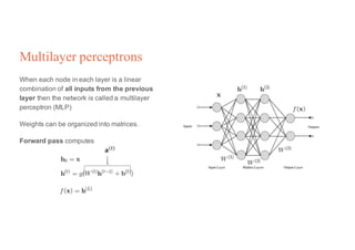
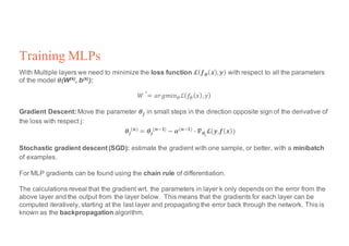
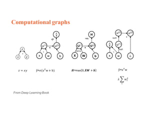
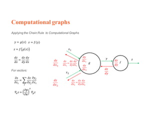
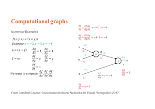
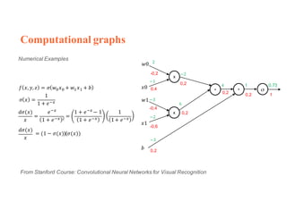
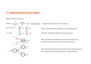
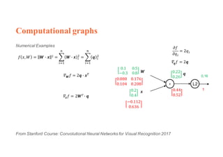
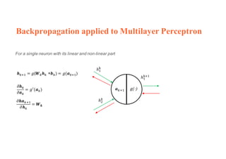
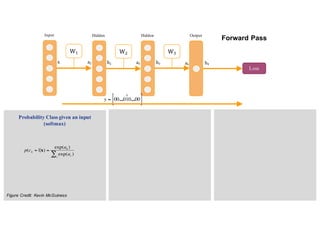
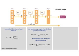
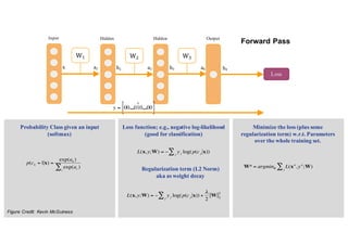
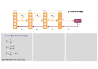
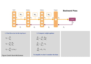
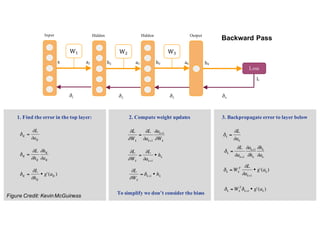
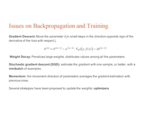
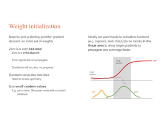
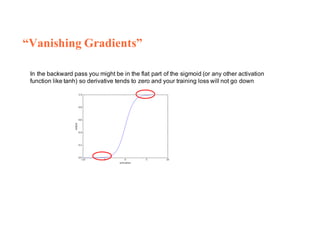
1. Backpropagation is an algorithm for training multilayer perceptrons by calculating the gradient of the loss function with respect to the network parameters in a layer-by-layer manner, from the final layer to the first layer. 2. The gradient is calculated using the chain rule of differentiation, with the gradient of each layer depending on the error from the next layer and the outputs from the previous layer. 3. Issues that can arise in backpropagation include vanishing gradients if the activation functions have near-zero derivatives, and proper initialization of weights is required to break symmetry and allow gradients to flow effectively through the network during training.

1. [course site]
Day 3 Lecture 1
Backpropagation
Elisa Sayrol

2. 2
Acknowledgements
Kevin McGuinness
kevin.mcguinness@dcu.ie
Research Fellow
Insight Centre for Data Analytics
Dublin City University

3. …in our last lecture

4. Multilayer perceptrons
When each node in each layer is a linear
combination of all inputs from the previous
layer then the network is called a multilayer
perceptron (MLP)
Weights can be organized into matrices.
Forward pass computes
𝐚(#)

5. Training MLPs
With Multiple layers we need to minimize the loss function 𝓛 𝒇 𝜽 𝒙 , 𝒚 with respect to all the parameters
of the model 𝜽(W(k), b(k)):
𝑊
∗
= 𝑎𝑟𝑔𝑚𝑖𝑛4ℒ 𝑓4 𝑥 , 𝑦
Gradient Descent: Move the parameter 𝜽𝒋 in small steps in the direction opposite sign of the derivative of
the loss with respect j:
𝜽𝒋
(𝒏) = 𝜽𝒋
(𝒏<𝟏) − 𝜶(𝒏<𝟏) @ 𝜵 𝜽𝒋
𝓛(𝒚,𝒇 𝒙 )
Stochastic gradient descent (SGD): estimate the gradient with one sample, or better, with a minibatch
of examples.
For MLP gradients can be found using the chain rule of differentiation.
The calculations reveal that the gradient wrt. the parameters in layer k only depends on the error from the
above layer and the output from the layer below. This means that the gradients for each layer can be
computed iteratively, starting at the last layer and propagating the error back through the network. This is
known as the backpropagation algorithm.

6. • Computational Graphs
• Examples applying chain of rule in simple graphs
• Backpropagation applied to Multilayer Perceptron
• Issues on Backpropagation and training
Backpropagation algorithm

7. Computational graphs
z
x y
x
u(1) u(2)
·
+
y^
x w b
σ
U(1) U(2)
matmul
+
H
X W b
relu
u(1)
u(2)
·
y^
x w λ
x
u(3)
sum
sqrt
𝑧 = 𝑥𝑦 𝑦C=𝜎(xFw + b) 𝑯=max 0, 𝑿𝑾 + 𝒃 𝑦C=xFw
𝜆 P 𝑤R
S
R
From Deep Learning Book

8. Computational graphs
Applying the Chain Rule to Computational Graphs
𝑦 = 𝑔(𝑥)
𝑧 = 𝑓 𝑔 𝑥
𝑑𝑧
𝑑𝑥
=
𝑑𝑧
𝑑𝑦
𝑑𝑦
𝑑𝑥
𝜕𝑧
𝜕𝑥R
= P
𝜕𝑧
𝜕𝑦V
𝜕𝑦V
𝜕𝑥RV
𝛻𝒙 𝑧 =
𝜕𝒚
𝜕𝒙
F
𝛻𝒚 𝑧
𝑑𝑧
𝑑𝑦
𝑑𝑦
𝑑𝑥X
𝑑𝑦
𝑑𝑥S
𝑑𝑧
𝑑𝑥X
𝑑𝑧
𝑑𝑥S
𝑑𝑧
𝑑𝑥X
=
𝑑𝑧
𝑑𝑦
𝑑𝑦
𝑑𝑥X
𝑑𝑧
𝑑𝑥S
=
𝑑𝑧
𝑑𝑦
𝑑𝑦
𝑑𝑥S
For vectors:
𝑥X
𝑥S
𝑦 𝑧
fg
𝑑𝑧
𝑑𝑦
𝑧 = 𝑓(𝑦)

9. Computational graphs
Numerical Examples
From Stanford Course: Convolutional Neural Networks for Visual Recognition 2017
+
x
𝑓 𝑥, 𝑦, 𝑧 = 𝑥 + 𝑦 𝑧
𝑥
𝑦
𝑧
𝑞
−2
5
−4
-12
3
𝑞 = 𝑥 + 𝑦
𝑓 = 𝑞𝑧
𝜕𝑞
𝜕𝑥
= 1
𝜕𝑞
𝜕𝑦
= 1
𝜕𝑓
𝜕𝑞
= 𝑧
𝜕𝑓
𝜕𝑧
= 𝑞
𝑊𝑒 𝑤𝑎𝑛𝑡 𝑡𝑜 𝑐𝑜𝑚𝑝𝑢𝑡𝑒:
𝜕𝑓
𝜕𝑥
,
𝜕𝑓
𝜕𝑦
,
𝜕𝑓
𝜕𝑧
𝐸𝑥𝑎𝑚𝑝𝑙𝑒 𝑥 = −2, 𝑦 = 5, 𝑧 = −4
𝜕𝑓
𝜕𝑓
= 1
𝜕𝑓
𝜕𝑓
= 1
1
𝜕𝑓
𝜕𝑞
= 𝑧 = −4
-4
𝜕𝑓
𝜕𝑧
= 𝑞 = 3
𝜕𝑓
𝜕𝑥
=
𝜕𝑓
𝜕𝑞
𝜕𝑞
𝜕𝑥
= −4 · 1 = −4
𝜕𝑓
𝜕𝑦
=
𝜕𝑓
𝜕𝑞
𝜕𝑞
𝜕𝑦
= −4 · 1 = −4
-4
-4
3

10. Computational graphs
Numerical Examples
x
+𝑓 𝑥, 𝑦, 𝑧 = 𝜎 𝑤k 𝑥k + 𝑤X 𝑥X + 𝑏
𝑤0
𝑥0
𝑏
x
𝑤1
𝑥1
+ σ
𝑑𝜎(𝑥)
𝑥
=
𝑒<m
1 + 𝑒<m 2
=
1 + 𝑒<m
− 1
1 + 𝑒<m
1
1+ 𝑒<m
𝜎 𝑥 =
1
1 + 𝑒<m
2
−1
−3
−2
−3
−2
6
4 1 0.73
1
𝑑𝜎(𝑥)
𝑥
= (1 − 𝜎(𝑥))(𝜎(𝑥))
0,20,2
0,2
-0,2
0,2
0,2
0,4
-0,4
-0,6
From Stanford Course: Convolutional Neural Networks for Visual Recognition

11. Computational graphs
Gates. Backward Pass
𝜎 𝑥 =
1
1 + 𝑒<m
𝑑𝜎(𝑥)
𝑥
= (1 − 𝜎(𝑥))(𝜎(𝑥))
𝑞 = 𝑥 + 𝑦 𝜕𝑞
𝜕𝑥
= 1
𝜕𝑞
𝜕𝑦
= 1
𝑓 = 𝑞𝑧
𝜕𝑓
𝜕𝑞
= 𝑧
𝜕𝑓
𝜕𝑧
= 𝑞
Sum: Distributes the gradient to both branches
Product: Switches gradient weigth values
Max: Routes the gradient only to the higher input
branche (not sensitive to the lower branche)
𝑥
𝑦
-0,2
0,2
0
max
2
1
2
+
In general: Derivative of a function
Add branches: Branches that split in the forward pass
and merge in the backward pass, add gradients

12. Computational graphs
Numerical Examples
From Stanford Course: Convolutional Neural Networks for Visual Recognition 2017
x
𝑓 𝑥, 𝑊 = 𝑾 @ 𝒙 2 = P 𝑾 @ 𝒙 R
S = P 𝒒 R
S
p
RqX
p
RqX
𝑾
𝒙
𝒒 0,16
𝜕𝑓
𝜕𝑞R
= 2𝑞R
1
𝛻 𝑾 𝑓 = 2𝒒 @ 𝒙F
L2
0.1 0.5
−0.3 0.8
0.2
0.4
0.22
0.26
0.44
0.52
0.088 0.176
0.104 0.208
𝛻𝒒 𝑓 = 2𝒒
𝛻𝒙 𝑓 = 2𝑾 𝑇 @ 𝒒
−0.112
0.636

13. Backpropagation applied to Multilayer Perceptron
For a single neuron with its linear and non-linear part
ℎX
w
g(·)
ℎS
x
ℎX
wyX
𝒂xyX
𝒉xyX = 𝑔(𝑾x 𝒉x +𝒃x) = 𝑔(𝒂xyX)
𝜕𝒉x
𝜕𝒂x
= 𝑔|(𝒂x)
𝜕𝒉𝒂xyX
𝜕𝒉x
= 𝑾 𝒌

14. Probability Class given an input
(softmax)
h2 h3a3 a4 h4
Loss
Hidden Hidden Output
W2 W3
x a2
Input
W1
Figure Credit: Kevin McGuiness
Forward Pass

15. Probability Class given an input
(softmax)
Loss function; e.g., negative log-likelihood
(good for classification)
h2 h3a3 a4 h4
Loss
Hidden Hidden Output
W2 W3
x a2
Input
W1
Regularization term (L2 Norm)
aka as weight decay
Figure Credit: Kevin McGuiness
Forward Pass

16. Probability Class given an input
(softmax)
Minimize the loss (plus some
regularization term) w.r.t. Parameters
over the whole training set.
Loss function; e.g., negative log-likelihood
(good for classification)
h2 h3a3 a4 h4
Loss
Hidden Hidden Output
W2 W3
x a2
Input
W1
Regularization term (L2 Norm)
aka as weight decay
Figure Credit: Kevin McGuiness
Forward Pass

17. 1. Find the error in the top layer:
h2 h3a3 a4 h4
Loss
Hidden Hidden Output
W2 W3
x a2
Input
W1
L
Figure Credit: Kevin McGuiness
Backward Pass

18. 1. Find the error in the top layer: 2. Compute weight updates
h2 h3a3 a4 h4
Loss
Hidden Hidden Output
W2 W3
x a2
Input
W1
L
Figure Credit: Kevin McGuiness
Backward Pass
To simplify we don’t consider the biass

19. 1. Find the error in the top layer: 3. Backpropagate error to layer below2. Compute weight updates
h2 h3a3 a4 h4
Loss
Hidden Hidden Output
W2 W3
x a2
Input
W1
L
Figure Credit: Kevin McGuiness
Backward Pass
To simplify we don’t consider the biass

20. Issues on Backpropagation and Training
Gradient Descent: Move the parameter 𝜃Vin small steps in the direction opposite sign of the
derivative of the loss with respect j.
𝜃(p) = 𝜃(p<X) − 𝛼 p<X @ 𝛻4ℒ 𝑦, 𝑓 𝑥 − 𝜆𝜃 p<X
Weight Decay: Penalizes large weights, distributes values among all the parameters
Stochastic gradient descent (SGD): estimate the gradient with one sample, or better, with a
minibatch of examples.
Momentum: the movement direction of parameters averages the gradient estimation with
previous ones.
Several strategies have been proposed to update the weights: optimizers

21. Weight initialization
Need to pick a starting point for gradient
descent: an initial set of weights
Zero is a very bad idea!
Zero is a critical point
Error signal will not propagate
Gradients will be zero: no progress
Constant value also bad idea:
Need to break symmetry
Use small random values:
E.g. zero mean Gaussian noise with constant
variance
Ideally we want inputs to activation functions
(e.g. sigmoid, tanh, ReLU) to be mostly in the
linear area to allow larger gradients to
propagate and converge faster.
0
tanh
Small
gradient
Large
gradient
bad good

22. In the backward pass you might be in the flat part of the sigmoid (or any other activation
function like tanh) so derivative tends to zero and your training loss will not go down
“Vanishing Gradients”

23. Note on hyperparameters
So far we have lots of hyperparameters to choose:
1. Learning rate (α)
2. Regularization constant (λ)
3. Number of epochs
4. Number of hidden layers
5. Nodes in each hidden layer
6. Weight initialization strategy
7. Loss function
8. Activation functions
9. …