CLASS X MATHS STATISTICS

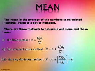
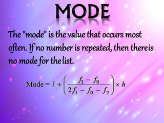
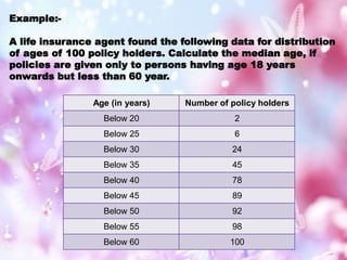
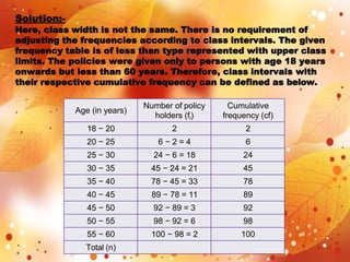
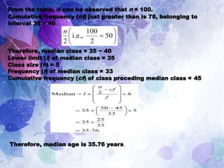
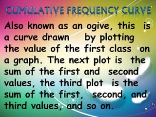
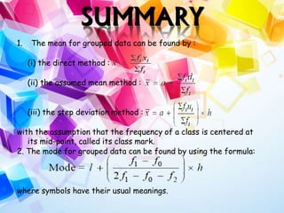
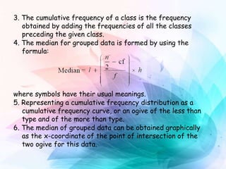
2. Statistics is the study of the collection,
organization, analysis, interpretation, and
presentation of data. It deals with all aspects of this,
including the planning of data collection in terms of
the design of surveys and experiments.
A statistician is someone who is particularly
well versed in the ways of thinking necessary for
the successful application of statistical analysis.
Such people have often gained this experience
through working in any of a wide number of fields.
There is also a discipline called mathematical
statistics that studies statistics mathematically.

3. The mean is the average of the numbers: a calculated
"central" value of a set of numbers.
There are three methods to calculate out mean and these
are:-

4. Example:-
A class teacher has the following absentee
record of 40 students of a class for the whole
term. Find the mean number of days a student
was absent.
Number of
days
0 − 6 6 − 10 10 − 14 14 − 20 20 − 28 28 −
38
38 − 40
Number of
students
11 10 7 4 4 3 1

5. To find the class mark of each interval, the following
relation is used.
Taking 17 as assumed mean (a), di and fidi are calculated as
follows.
Solution:-
Number of days Number of
students fi
xi di = xi − 17 fidi
0 − 6 11 3 − 14 − 154
6 − 10 10 8 − 9 − 90
10 − 14 7 12 − 5 − 35
14 − 20 4 17 0 0
20 − 28 4 24 7 28
28 − 38 3 33 16 48
38 − 40 1 39 22 22
Total 40 − 181

6. From the table, we obtain
Therefore, the mean number of days is 12.48 days for which a
student was absent.

7. LIMITATION:- Disadvantage of themean:Themajor disadvantage,
which doesnot always occur, isthe fact that a mean can be
dramatically affected byoutliers in theset.Forexample, if we find
the mean of the set of numbers 1, 2, 3, 4, 5 we get 3.
However, when we dramatically alter one number in thesetand
find the average again, the mean isquite different. Forexample 1,
2, 3, 4, 20 has a mean of 6.
Uses:- the mean to describe the middle of a set of data that
does not have an outlier.

8. The "mode" is the value that occurs most
often. If no number is repeated, then thereis
no mode for thelist.

9. Limitation:-Could be very far from the actual
middle of the data. The least reliable way to find the
middle or average of the data.
Uses:- the mode when the data is non-numeric or
when asked to choose the most popular item.

10. Example:-
The given distribution shows the number of runs
scored by some top batsmen of the world in one-
day international cricket matches.
Find the mode of the data.
Runs scored Number of batsmen
3000 − 4000 4
4000 − 5000 18
5000 − 6000 9
6000 − 7000 7
7000 − 8000 6
8000 − 9000 3
9000 − 10000 1
10000 − 11000 1

11. Solution:-
From the given data, it can be observed that the maximum
class frequency is 18, belonging to class interval 4000 −
5000.
Therefore, modal class = 4000 − 5000
Lower limit (l) of modal class = 4000
Frequency (f1) of modal class = 18
Frequency (f0) of class preceding modal class = 4
Frequency (f2) of class succeeding modal class = 9
Class size (h) = 1000
Therefore, mode of the given data is 4608.7 run

12. The "median" is the "middle"
value in the list of numbers. To
find the median, your numbers
have to be listed in numerical
order, so you may have to
rewrite your list first.

13. LIMITATION: If the gap between some numbers is large,
while it is small between other numbers in the data, this can
cause the median to be a very inaccurate way to find the
middle of a set of values.
Uses:- the median to describe the middle of a set of data
that does have an outlier.

14. Example:-
A life insurance agent found the following data for distribution
of ages of 100 policy holders. Calculate the median age, if
policies are given only to persons having age 18 years
onwards but less than 60 year.
Age (in years) Number of policy holders
Below 20 2
Below 25 6
Below 30 24
Below 35 45
Below 40 78
Below 45 89
Below 50 92
Below 55 98
Below 60 100

15. Solution:-
Here, class width is not the same. There is no requirement of
adjusting the frequencies according to class intervals. The given
frequency table is of less than type represented with upper class
limits. The policies were given only to persons with age 18 years
onwards but less than 60 years. Therefore, class intervals with
their respective cumulative frequency can be defined as below.
Age (in years)
Number of policy
holders (fi)
Cumulative
frequency (cf)
18 − 20 2 2
20 − 25 6 − 2 = 4 6
25 − 30 24 − 6 = 18 24
30 − 35 45 − 24 = 21 45
35 − 40 78 − 45 = 33 78
40 − 45 89 − 78 = 11 89
45 − 50 92 − 89 = 3 92
50 − 55 98 − 92 = 6 98
55 − 60 100 − 98 = 2 100
Total (n)

16. From the table, it can be observed that n = 100.
Cumulative frequency (cf) just greater than is 78, belonging to
interval 35 − 40.
Therefore, median class = 35 − 40
Lower limit (l) of median class = 35
Class size (h) = 5
Frequency (f) of median class = 33
Cumulative frequency (cf) of class preceding median class = 45
Therefore, median age is 35.76 years.

17. Also known as an ogive, this is
a curve drawn by plotting
the value of the first class on
a graph. The next plot is the
sum of the first and second
values, the third plot is the
sum of the first, second, and
third values, and so on.

18. Example:-
During the medical check-up of 35 students of a class, their
weights were recorded as follows:
Weight (in kg) Number of students
Less than 38 0
Less than 40 3
Less than 42 5
Less than 44 9
Less than 46 14
Less than 48 28
Less than 50 32
Less than 52 35
Draw a less than type ogive for the given data. Hence obtain the
median weight from the graph verify the result by using the
formula.

19. Weight (in kg)
upper class limits
Number of students
(cumulative frequency)
Less than 38 0
Less than 40 3
Less than 42 5
Less than 44 9
Less than 46 14
Less than 48 28
Less than 50 32
Less than 52 35
Solution:-
The given cumulative frequency distributions of less than type are
Taking upper class limits on x-axis and their respective cumulative
frequencies on y-axis, its ogive can be drawn as follows.

20. Here, n = 35
So, = 17.5
Mark the point A whose ordinate is 17.5 and its x-coordinate is
46.5. Therefore, median of this data is 46.5.

21. It can be observed that the difference between two consecutive
upper class limits is 2. The class marks with their respective
frequencies are obtained as below.

22. Weight (in kg) Frequency (f) Cumulative
frequency
Less than 38 0 0
38 − 40 3 − 0 = 3 3
40 − 42 5 − 3 = 2 5
42 − 44 9 − 5 = 4 9
44 − 46 14 − 9 = 5 14
46 − 48 28 − 14 = 14 28
48 − 50 32 − 28 = 4 32
50 − 52 35 − 32 = 3 35
Total (n) 35
The cumulative frequency just greater than is 28,
belonging to class interval 46 − 48.
Median class = 46 − 48
Lower class limit (l) of median class = 46

23. Frequency (f) of median class = 14
Cumulative frequency (cf) of class preceding median class = 14
Class size (h) = 2
Therefore, median of this data is 46.5.
Hence, the value of median is verified.

24. 1. The mean for grouped data can be found by :
(i) the direct method :
(ii) the assumed mean method :
(iii) the step deviation method :
with the assumption that the frequency of a class is centered at
its mid-point, called its class mark.
2. The mode for grouped data can be found by using the formula:
where symbols have their usual meanings.

25. 3. The cumulative frequency of a class is the frequency
obtained by adding the frequencies of all the classes
preceding the given class.
4. The median for grouped data is formed by using the
formula:
where symbols have their usual meanings.
5. Representing a cumulative frequency distribution as a
cumulative frequency curve, or an ogive of the less than
type and of the more than type.
6. The median of grouped data can be obtained graphically
as the x-coordinate of the point of intersection of the
two ogive for this data.