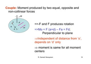
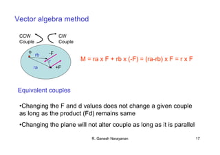
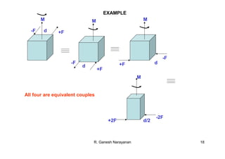
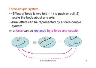
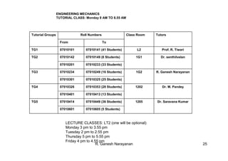
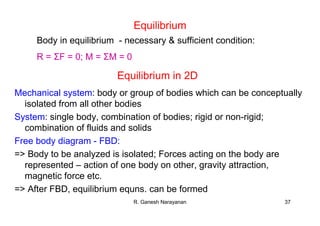
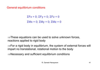
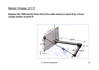
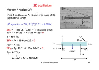
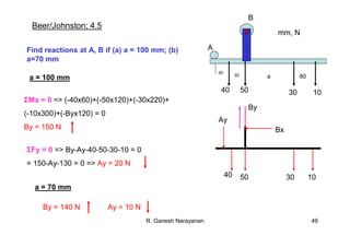
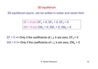
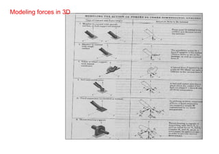
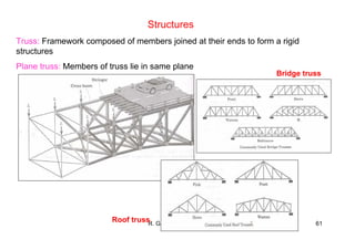
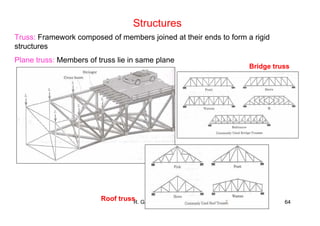
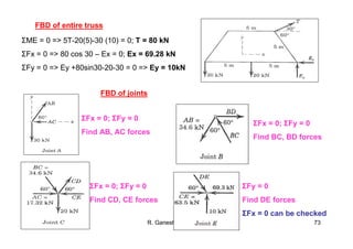
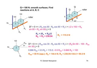
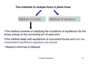
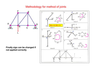
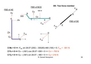
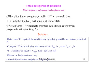
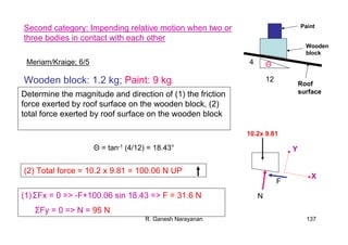
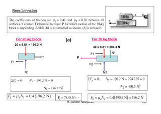
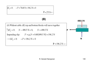
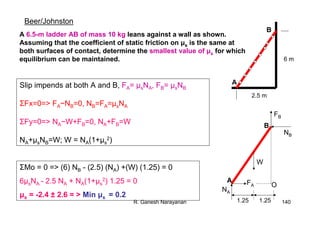
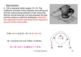
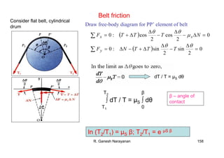
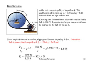
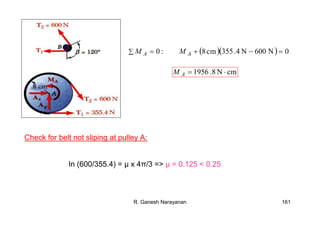
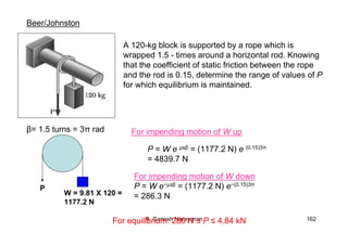
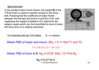
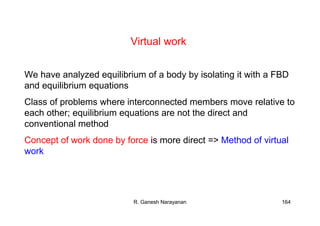
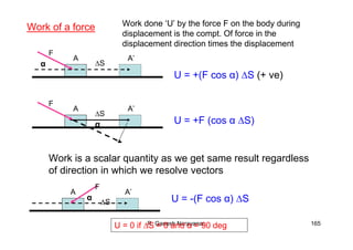
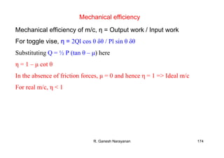
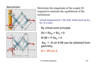
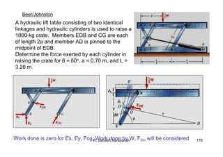
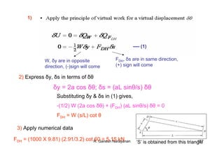
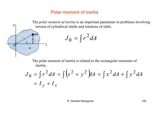
This document contains lecture slides for a statics course taught by R. Ganesh Narayanan at IIT Guwahati. It introduces engineering mechanics and statics concepts like forces, moments, couples, and resultants. It provides examples and references textbooks on statics and dynamics by authors like Beer and Johnston, Meriam and Kraige, and Shames. The slides were prepared by R. Ganesh Narayanan and contain theories, figures, problems and concepts from the referenced textbooks to teach a 1st year undergraduate statics course.


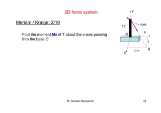
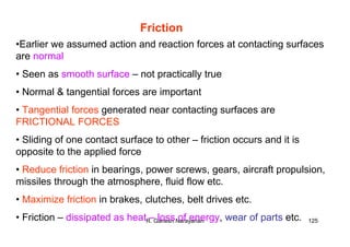
![R. Ganesh Narayanan 45
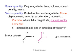
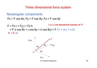
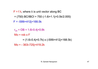
F = T = ITI nAB = 10 [12i-15j+9k/21.21] = 10(0.566i-0.707j+0.424k) k N
Mo = rxF = 15j x 10(0.566i-0.707j+0.424k) = 150 (-0.566k+0.424i) k Nm
Mz = Mo.k= 150 (-0.566k+0.424i).k = -84.9 kN. m](https://image.slidesharecdn.com/mechanicsfullnotes-190822164707/85/Mechanics-full-notes-45-320.jpg)

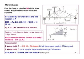
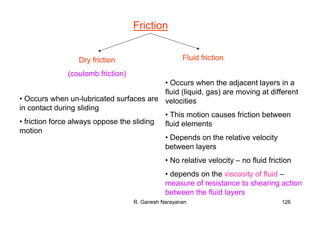
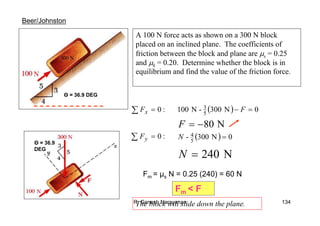
![R. Ganesh Narayanan 58
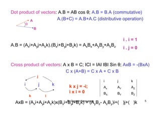
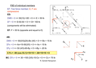
F.B.D. - 1
F.B.D. - 2
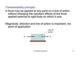
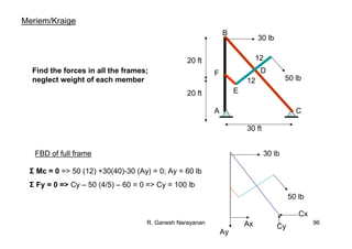
ΣMc = 0 => (Dy) (15) – 200 (15) (15/2) –
(1/2)(15)(300)[2/3 (15)] = 0
Dy = 3000 N
F.B.D. - 2](https://image.slidesharecdn.com/mechanicsfullnotes-190822164707/85/Mechanics-full-notes-58-320.jpg)
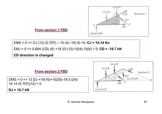
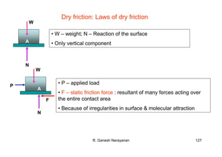
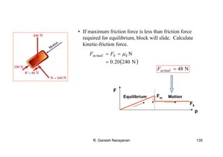
![R. Ganesh Narayanan 59
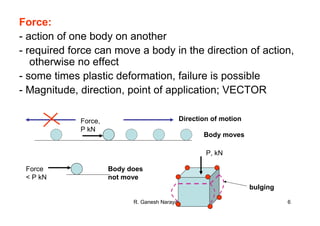
F.B.D. - 1
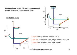
ΣMB = 0 => -Ay (13) +(3000) (21) – 200
(34) (34/2-13) – ½ (300) (15) [6+2/3(15)]
= 0
Ay = -15.4 N
ΣFy = 0 => Ay+By+3000-200(34)-
(1/2)(300)(15) = 0
Sub. ‘Ay’ here,
=> By = 6065 N](https://image.slidesharecdn.com/mechanicsfullnotes-190822164707/85/Mechanics-full-notes-59-320.jpg)


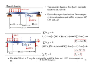
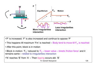
![R. Ganesh Narayanan 107
x
y
h
xy
dy
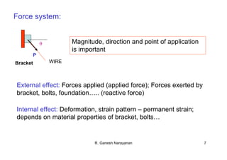
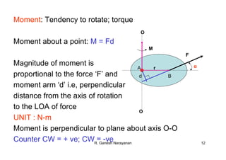
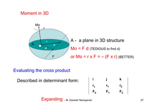
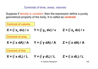
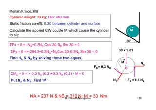
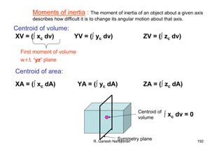
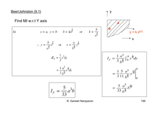
Find the y-coordinate of centroid of the triangular area
AY = ∫ y dA
½ b h (y) = ∫ y (x dy) = ∫ y [b (h-y) / h] dy = b h2 / 6
b
X / (h-y) = b/h
0
h
0
h
Y = h / 3](https://image.slidesharecdn.com/mechanicsfullnotes-190822164707/85/Mechanics-full-notes-107-320.jpg)

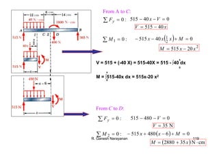

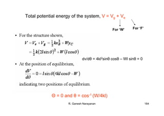
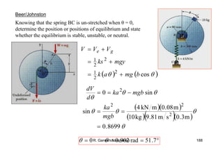
![R. Ganesh Narayanan 186
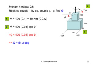
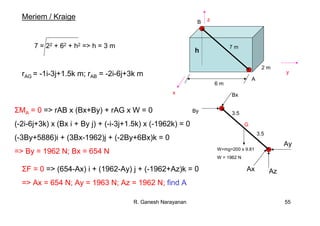
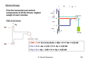
Meriam/Kraige, 7/39
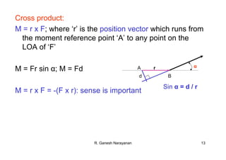
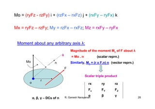
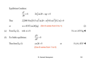
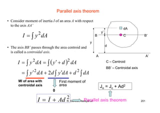
For the device shown the spring would be un-stretched
in the position θ=0. Specify the stiffness k of the spring
which will establish an equilibrium position θ in the
vertical plane. The mass of links are negligible.
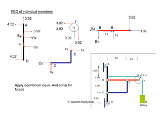
Spring stretch distance, x = 2b-2b cos θ
Ve = ½ k [(2b)(1-cos θ)]2 = 2kb2 (1-cos θ)2
Vg = -mgy = -mg (2bsinθ) = -2mgbsin θ
V = 2kb2 (1-cos θ)2 - 2mgbsin θ
For equilibrium, dv / dθ = 4kb2(1-cos θ) sin θ - 2mgb cosθ = 0
=> K = (mg/2b) (cot θ/1-cos θ)
k
b b
b
θ
m
y
Vg = 0](https://image.slidesharecdn.com/mechanicsfullnotes-190822164707/85/Mechanics-full-notes-187-320.jpg)
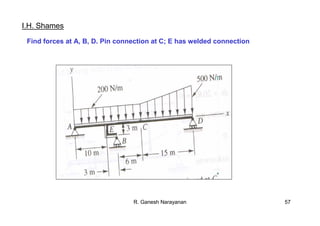
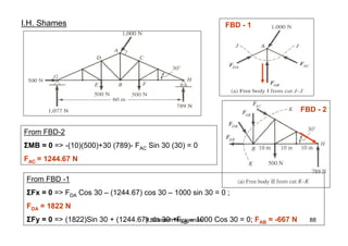
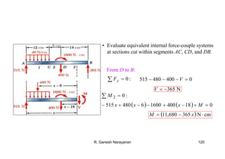
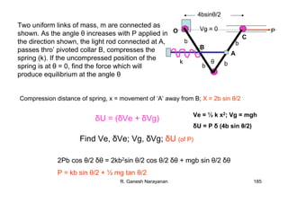
![R. Ganesh Narayanan 205
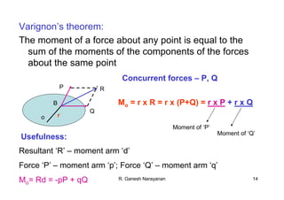
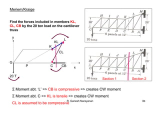
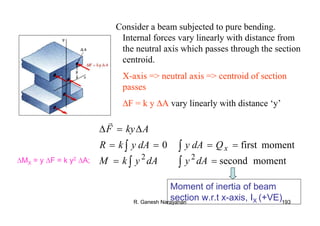
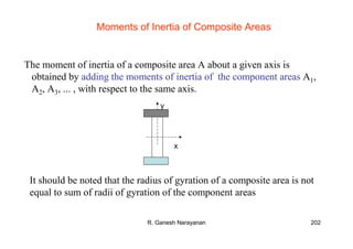
Find the centroid of the area of the un-equal Z section. Find the
moment of inertia of area about the centroidal axes
shames
Ai xi yi Aixi Aiyi
2x1=2 1 7.5 2 15
8x1=8 2.5 4 20 32
4x1=4 5 0.5 20 2
ΣAi = 14 ΣAixi = 42 ΣAiyi = 49
1
2
3
Xc = 42/14 = 3 in.; Yc = 49/14 = 3.5in
y
x
1
6
2 1 4
1
1
2
3
Xc, Yc
Ixcxc = [(1/12)(2)(13)+(2)(42)] + [(1/12)(1)(83)+(8)(1/2)2] +
[(1/12)(4)(13)+(4)(32)] = 113.16 in4
Similarly, Iycyc = 32.67 in4](https://image.slidesharecdn.com/mechanicsfullnotes-190822164707/85/Mechanics-full-notes-206-320.jpg)
![R. Ganesh Narayanan 208
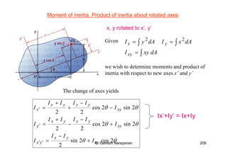
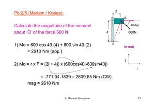
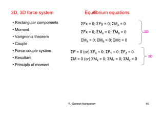
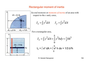
Product of inertia, Ixy
∫= dAxyI xy
[Similar to Ixx (or Ix), Iyy (or Iy)]
When the x axis, the y axis, or both are an axis of symmetry,
the product of inertia is zero.
The contributions to Ixy of dA and dA’ will cancel out
Parallel axis theorem for products of inertia:
AyxII xyxy +=
Centroid ‘C’ is defined by x, y](https://image.slidesharecdn.com/mechanicsfullnotes-190822164707/85/Mechanics-full-notes-209-320.jpg)