This document discusses various methods for measuring disease frequency and trends. It defines key epidemiological terms like prevalence, incidence, odds ratio, and relative risk. It explains how to calculate these measures and interpret them. For example, it shows how to calculate the odds ratio from a 2x2 table to measure the association between alcohol use and accidents. It also discusses factors that can indicate a causal relationship and gives examples of time series analysis of disease trends over time.

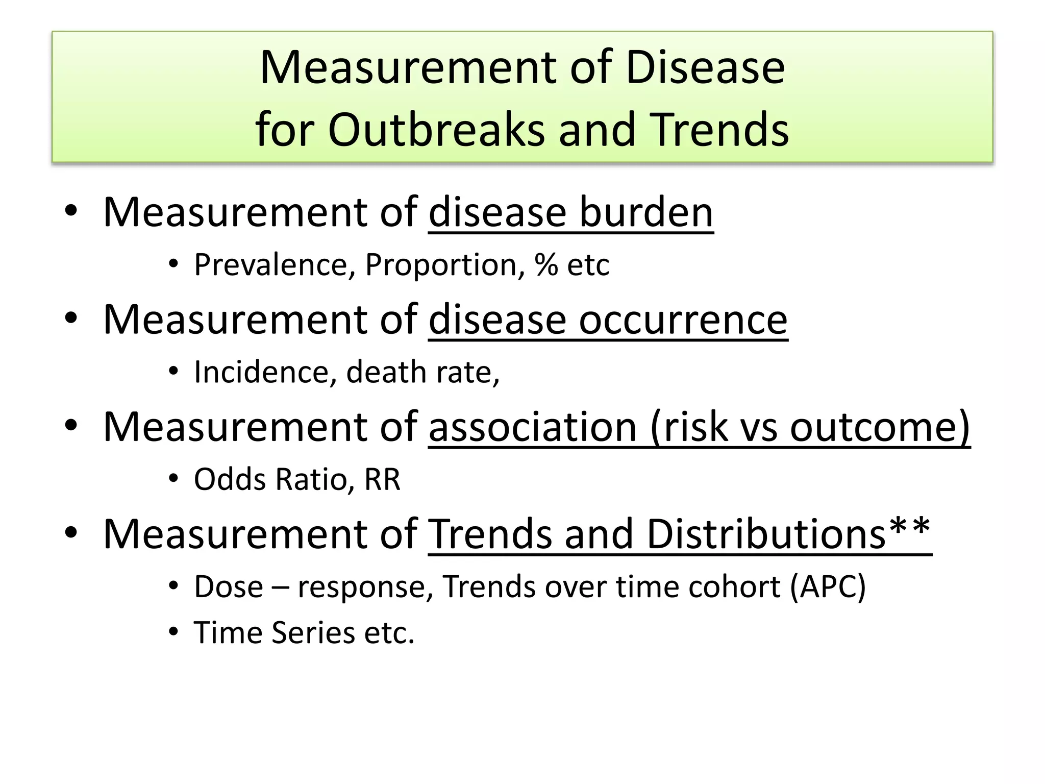
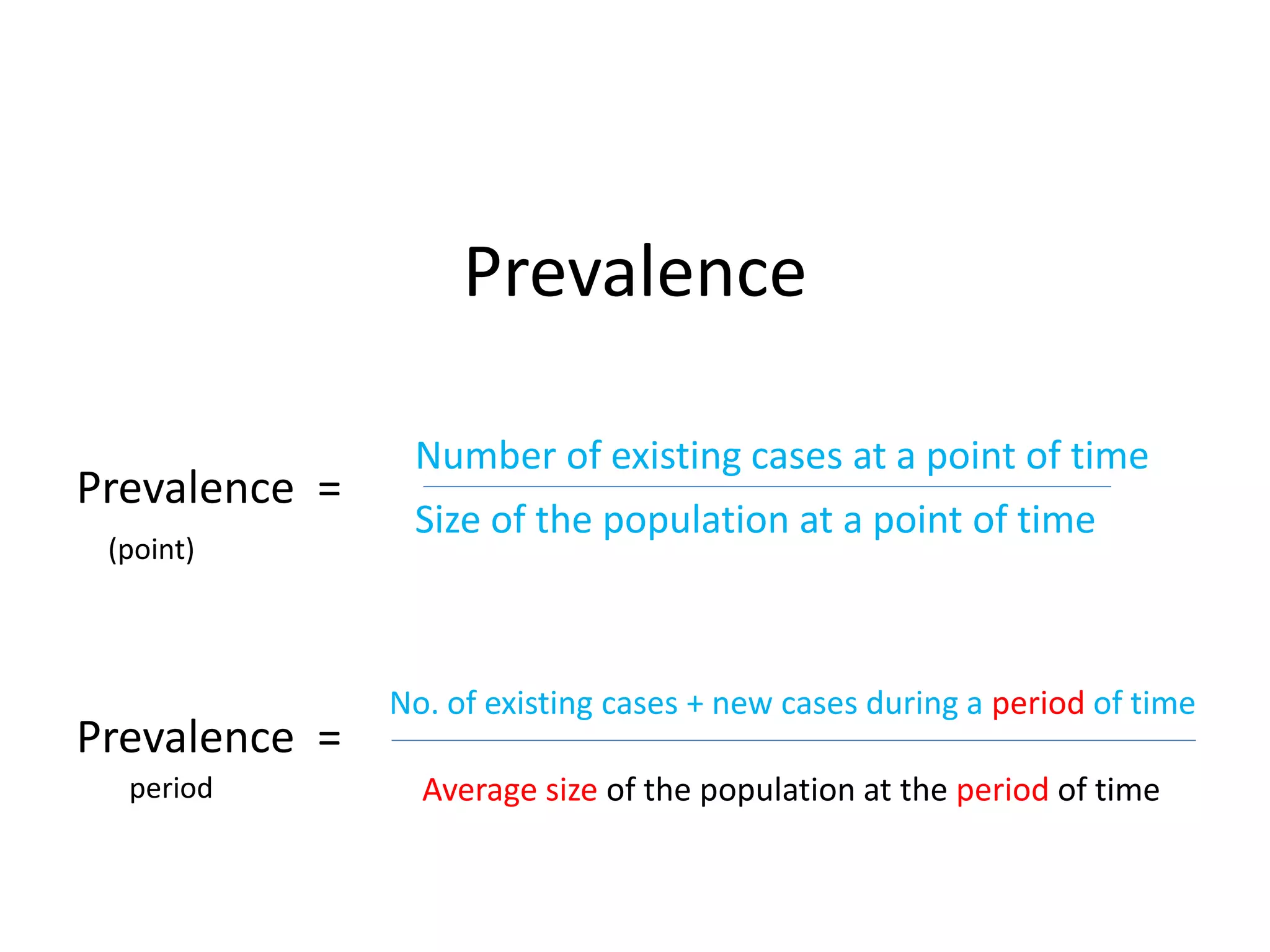
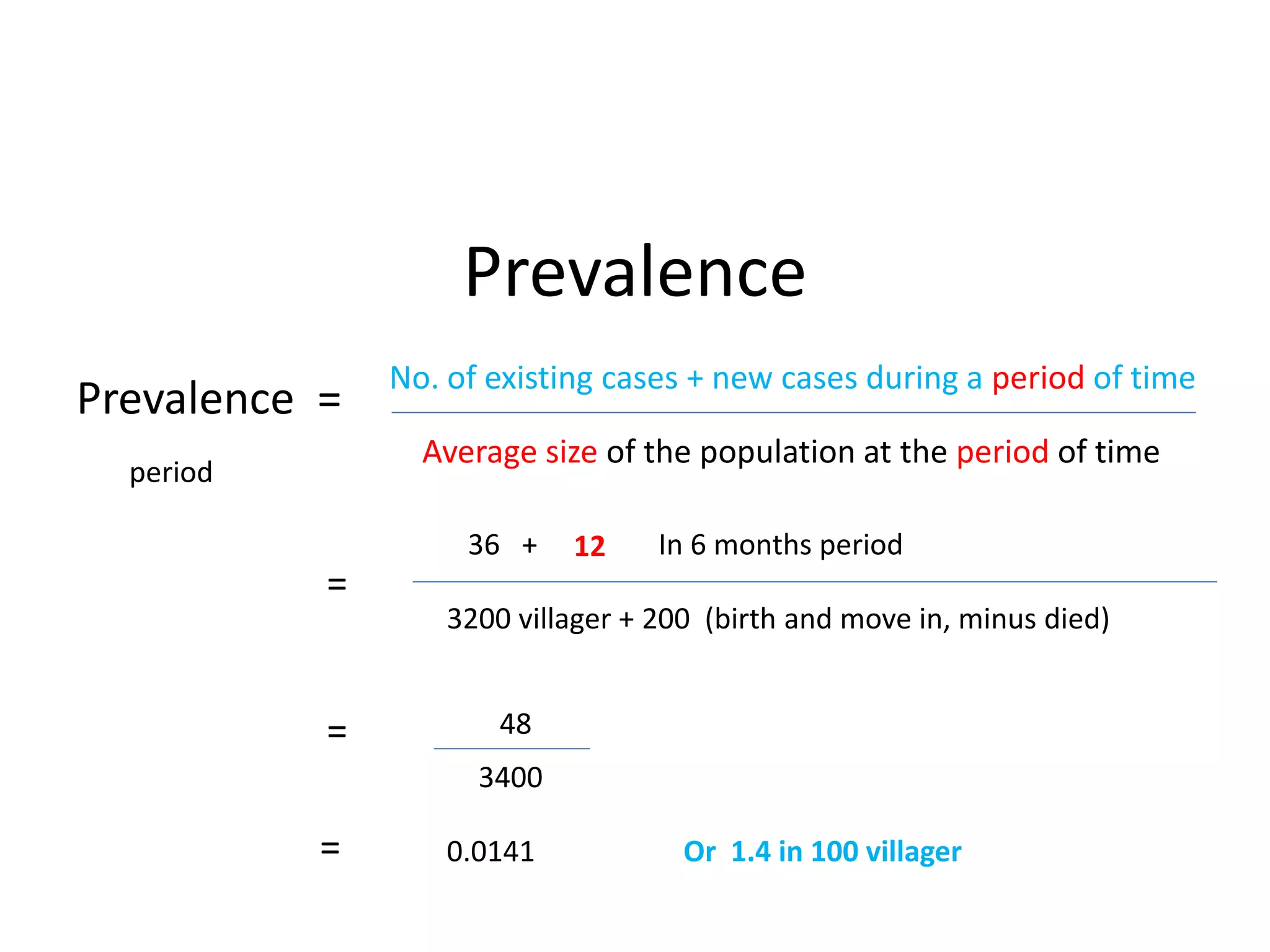
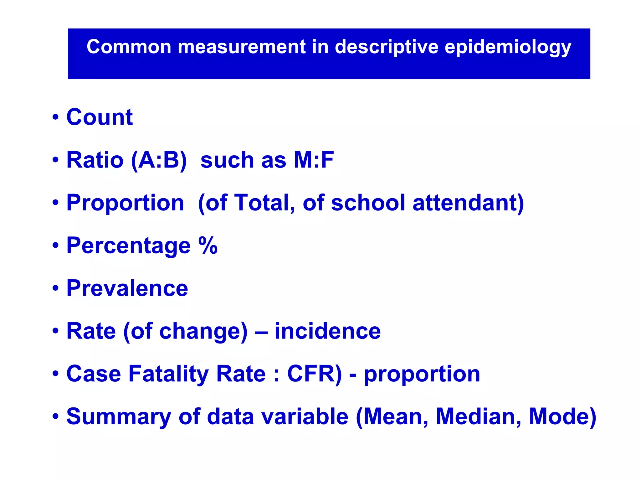
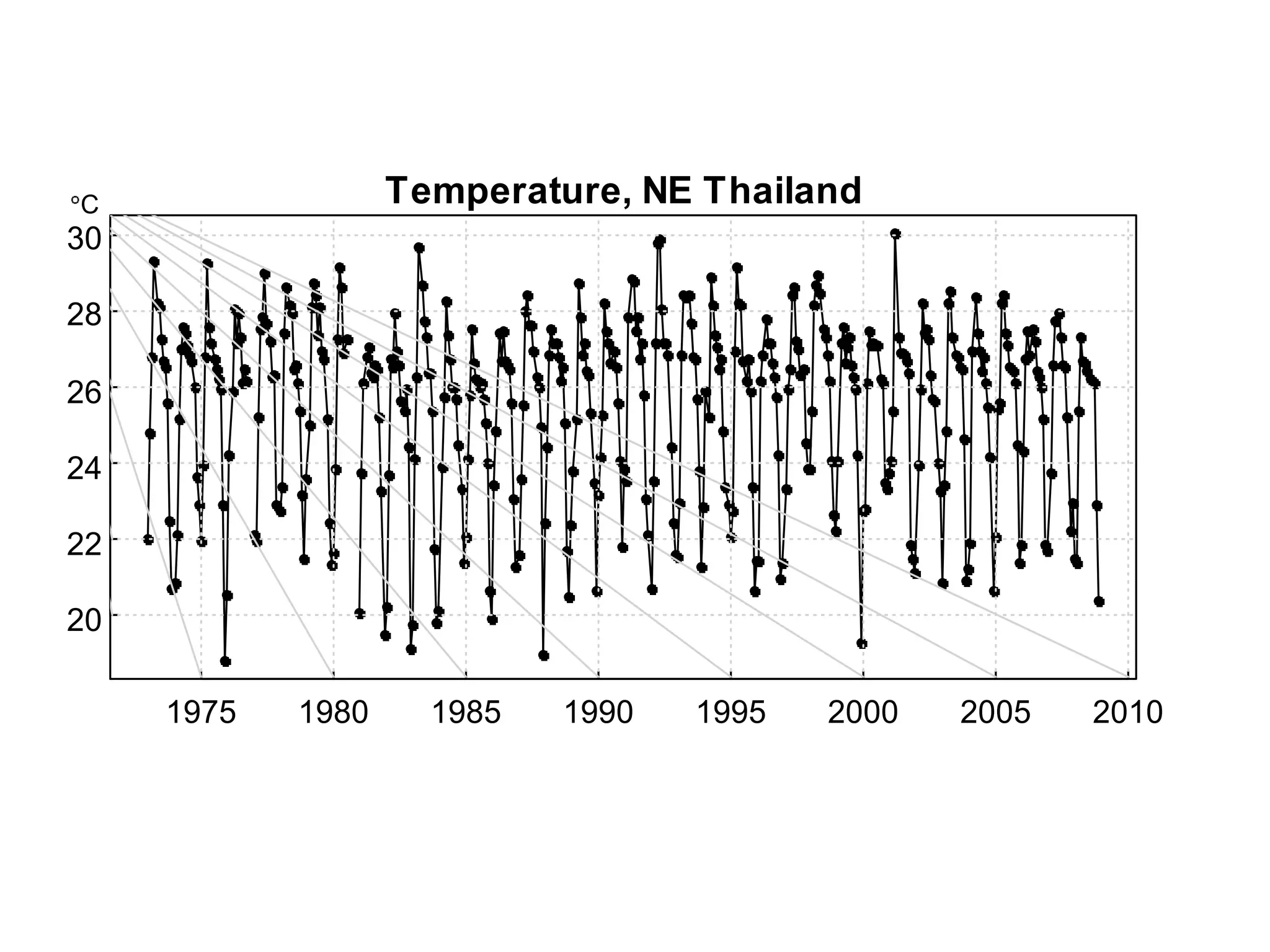
1. Measurement of Disease
Frequency
Occurrence and Trends
Module 1

2. Measurement of Disease
for Outbreaks and Trends
• Measurement of disease burden
• Prevalence, Proportion, % etc
• Measurement of disease occurrence
• Incidence, death rate,
• Measurement of association (risk vs outcome)
• Odds Ratio, RR
• Measurement of Trends and Distributions**
• Dose – response, Trends over time cohort (APC)
• Time Series etc.

3. Measurement of disease burden
• Count (number) and unit of count (such as
aggregate number – group, cluster, flock etc)
• Count and proportion (number of case per
survey population, %, ratio – m:f)
• Prevalence (magnitude)

4. Prevalence
Prevalence =
Number of existing cases at a point of time
Average size of the population at the period of time
Prevalence =
No. of existing cases + new cases during a period of time
Size of the population at a point of time
(point)
period

5. Prevalence (point)
Prevalence =
Number of DM cases in the survey of a village
Size of the population of the village
(point)
=
36
3200 villager
= 0.01125 Or 1.12 person in 100 people

6. Prevalence
Average size of the population at the period of time
Prevalence =
No. of existing cases + new cases during a period of time
period
=
36 + 12 In 6 months period
3200 villager + 200 (birth and move in, minus died)
= 48
3400
= 0.0141 Or 1.4 in 100 villager

7. Measurement of disease occurrence
Incidence (rate) =
No. of FMD in cows in 1 year
Size of population at risk who stay in the area in 1 year
=
New cases occur in an observed period ( 1 year)
Population of cows in the province in 1 year
=
500
2500
= 200 FMD per 1000 Cows per year
X 1000 or 100000
X 10000
Incidence is rate of change : unit of calculation is per time (t minus 1)
(incidence rate, death rate etc.

8. Common measurement in descriptive epidemiology
• Count
• Ratio (A:B) such as M:F
• Proportion (of Total, of school attendant)
• Percentage %
• Prevalence
• Rate (of change) – incidence
• Case Fatality Rate : CFR) - proportion
• Summary of data variable (Mean, Median, Mode)

9. Number of patients with “D” disease reported from
all hospitals in Province/Division ‘M’ by week, in 201X
Hospital
Area Total 1 2 3 4 5 6 7 8 9 10 11 12 13 14 15 16 17 18 19 20
Provineial H 1778 112 112 101 101 112 116 100 101 127 123 89 85 87 103 63 86 75 68 7
Hosp A 163 28 31 26 28 13 12 9 5 11
Hosp B 5 1 1 1 1 1
Hosp C 169 24 16 14 22 25 23 20 4 1 2 16
Hosp D 656 44 37 48 44 27 21 43 24 24 19 14 39 28 43 41 45 34 39 28
Hosp E 466 19 33 36 38 28 20 40 23 16 21 27 16 21 21 14 27 18 24 22
Hosp F 226 17 17 26 23 47 26 41 22 2
Hosp G 242 27 18 25 33 21 20 33 18 28 17 1

10. Understand sources of data
and how data collected
• Definition of case required for notification
• Surveillance and reporting system (and
requirement – such as priority/urgent etc)
• Reporting Persons, organization
• Timeliness
• Completion
• Evaluation and supervision
• Technology

11. Previous slide content show
• Count per week
• Count of cases among different hospital/area
• No report and missing data
• Incomplete information in some data
• No information, no data – difficult to analyze or
interpretation
• No population in each area make it hard to
compare the problem
• Can we say something about the trends of
disease?

12. John Snow : Observation and study of
Cholera Outbreak, London 1854

13. Cholera cases, rate per HH
By water supplied company, London 1854.
Southwark & Vauxhall 40,046 1,263 315
Company
Lamberth Company 26,107 98 37
Rest of London 256,423 1,422 59
Tap water
Supplied company
No. HH cases
Case per
10000 HH

14. Measure of disease transmission

15.  Index – first case identified
 Primary – case that brings the infection into a population
 Secondary – infected by a primary case
 Tertiary – infected by a secondary case
P
S
S
T
Susceptible
Immune
Asymptomatic
Clinical
S
T
การถ่ายทอดโรค (Disease Transmission)

16. Transmission: Reproductive Number
Basic Reproductive Number (R zero)
Secondary cases occurred as a result of
exposure (contact) to indexed cases or
previous case
Ro = between 1-2 from this example

17. After an ILI index case ill in families
no. of new cases sick in 1 incubation period
Size of families New case occur Index to new case ratio
5 2 1:2
4 2 1:2
3 1 1:1
6 3 1:3

18. Estimated Ro
in selected infectious disease
• Seasonal Influenza (2-4)
• Pandemic A/H1N1 (2-5)
• H5N1 (0.5-2)
• SARs (3-7****)
• Tuberculosis (1-2)***
• MERS (0.7-4**)
• Ebola (1-5**)
• HFMD (1-6**)
** depend on settings, family size, contact methods, procedure

19. First MERS in Korea and transmission

20. Transmission Relationships

21. Measurement of association (risk vs outcome)
Odds Ratio, RR
Terminology
• Variable (things with information of interest : Sex,
age, Blood sugar, Infection (Y/N), eat food A, bite by
rabid dog, vaccination) (y/n)……etc)
• Association ( possible relationship of x and y)
• Correlation (how x and y go together) (+/-)
• Some association can be cause-effect
relationship

22. Measurement of association (risk vs outcome)
Odds Ratio, RR
Association
• What is Odd and Odds Ration
a:b is Odd of X ( c:d is another odd of Y)
X:Y is Odds Ratio
• What is Relative Risk (similar concept
“Studies showed “Drink alcohol” associated with increase in road accident by 3 times”

23. Calculation format Odd, Odds Ratio
Accident No accident
Drinking “alcohol”
Over 75 mg%
a b a+b
No alcohol c d c+d
a+c b+d N = a+b+c+d

24. Accident No accident
Drinking “alcohol”
Over 75 mg%
a b a+b
No alcohol c d c+d
a+c b+d N =
a+b+c+d
Odd of accident in drinking = a/b
Odd of accident in No drinking = c/d
Odd Ratio of Alcohol in accident = (a/b) /(c/d) = a*d /b*c
ORs = number
+ Calculate 95% Confident Intervals

25. Accident No accident
Drinking “alcohol”
Over 75 mg%
50 500 550
No alcohol 5 1200 1205
55 1700 1755
Odd of accident in drinking = a/b = 50/500 = 0.1
Odd of accident in No drinking = c/d = 5/1200 = 0.00416
Odd Ratio of Alcohol in accident = (0.1) /(0.00416) = 24.04 times
ORs = number
+ Calculate 95% Confident Intervals

26. Calculation format RR, RRs Ratio
Case Measles Normal (child) no
illness
MMR vaccination
a b a+b
No MMR
vaccination
c d c+d
a+c b+d N = a+b+c+d

27. Case Measles Normal (child) no
illness
MMR vaccination a b a+b
No MMR
vaccination
c d c+d
a+c b+d N = a+b+c+d
RR of disease in vaccination = a/a+b
RR of disease in non-vaccination = c/c+d
RRs Ratio is = a(a+b)/(c /(c+d))

28. Case Measles Normal (child) no
illness
MMR vaccination 5 400 405
No MMR
vaccination
28 300 328
33 730 763
RR of disease in vaccination = a/a+b = 5/405 = 0.012
RR of disease in non-vaccination = c/c+d = 28/328 = 0.0853
RRs Ratio is = a(a+b)/(c /(c+d))
= 0.012/0.0853 = 0.14
MMR vaccination has 7.1 time protective effect or approximately 76 % efficacy

29. Cause-effect Association
• Strength of association (high RRs, Ors)
• Consistency
• Specificity
• Temporal relation (A happened before disease)
• Biological Plausibility
• Dose-response relationship
• Coherence
• Experiment support
• Analogy **
** too weak , may not be necessary

30. Q/A
Thank you

31. Trends Analysis (advance)
For your interest only
For use in future

32. Time series analysis

33. Temperature, NE Thailand
1975 1980 1985 1990 1995 2000 2005 2010
20
22
24
26
28
30
C

34. Main composition of determinants
of a Time Series
• Trend: linear, curvinear, moving average
• Oscillation (cosine function)
– Harmonic terms e.g. cos(a), cos(2a)
– Starting points e.g. cos(m+a), cos(n+2a)
• Autoregressive effect
– Preceding status has effects on the current one.
• Optionally other explanatory independent terms e.g.
temperature, rainfalls, which are beyond the trend
and cyclical effects
• Random errors

35. Temperature, NE Thailand
1975 1980 1985 1990 1995 2000 2005 2010
20
22
24
26
28
30
C
Analysis : Output from R program - red line show
trend of temperature with seasonal (time) variation

36. 202224262830
observed
25.025.526.026.5
trend
-4-3-2-1012
seasonal
-3-101234
1975 1980 1985 1990 1995 2000 2005 2010
random
Time
Decomposition of additive time series

37. Forecasting malaria in Yalamalaria
2000 2005 2010 2015
0
500
1000
1500

38. การเปลี่ยนแปลงหลังการระบาดใหญ่ ๕ ปี ของไข้หวัดใหญ่สายพันธ์ใหม่ 2009

39. Age-Period-Cohort (APC)
• Age – risk of disease depend on age such as
– Low immunity in children
– Exposure to chemical, hormone change
– Age related disease, elderly less immunity etc
• Period : certain period living aspect change (60s,
80s, 90s, 2000s, 2010….)
• Cohort : Birth cohort experienced different
era/period
• Interaction for risk factors

40. Hutcha Sriplung Thai Network of Cancer Registries 40
Female breast cancer in Thailand
Year
1989199019911992199319941995199619971998199920002001200220032004200520062007
0
5
10
15
20
25
30
Breast Cancer
Thailand, 1989-2007
Chiang Mai
Lampang
Khon Kaen
Songkhla
Year
ASR(per100000population

41. Hutcha Sriplung Thai Network of Cancer Registries 41
Male colo-rectal cancer in Thailand
89 90 91 92 93 94 95 96 97 98 99 00
0
5
10
15
20
25
Chiang Mai
Lampang
Khon Kaen
Songkhla
Year
ASR /100,000 population

42. Hutcha Sriplung Thai Network of Cancer Registries 42
Tobacco consumption and lung cancer
in Australia
1945
1947
1949
1951
1953
1955
1957
1959
1961
1963
1965
1967
1969
1971
1973
1975
1977
1979
1981
1983
1985
1987
1989
1991
1993
1995
1997
0.0
10.0
20.0
30.0
40.0
50.0
60.0
70.0
80.0
Lung Cancer-Male
Lung Cancer-Female
Tobacco consumption
3.0
1.5
0.0
2.0
1.0
2.5
Tobacco
Kg/capita
Death/100,000
population
Year
AIHW: deloop M & Bhatia K 2001: Australian Health Trends 2001. AIHW Cat. No. PHE 24. Canberra: AIHW; the National Mortality
Database.
~20 years

43. The End – Thank you