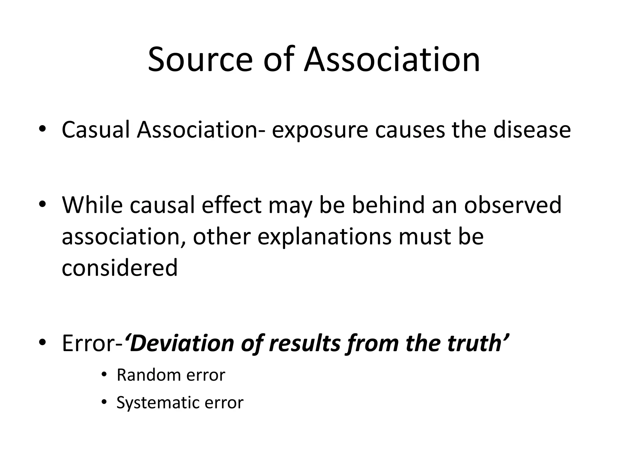
This document discusses various types of bias and confounding that can occur in epidemiological studies, including: 1) Selection bias, information bias, and confounding can all introduce systematic error and invalidate study results. Selection bias occurs when individuals have different probabilities of being included based on exposure or outcome. Information bias is misclassification of exposure or outcome. 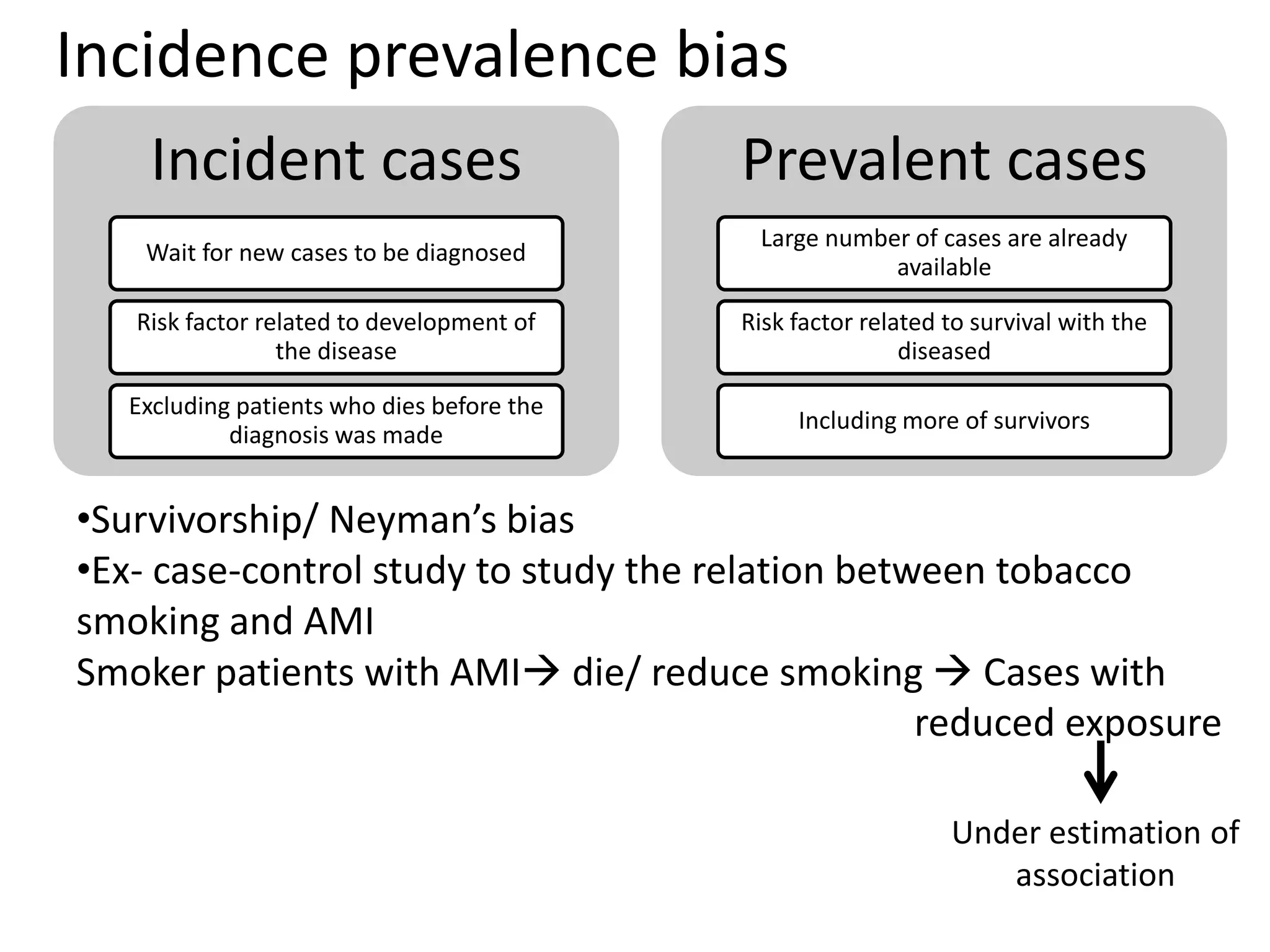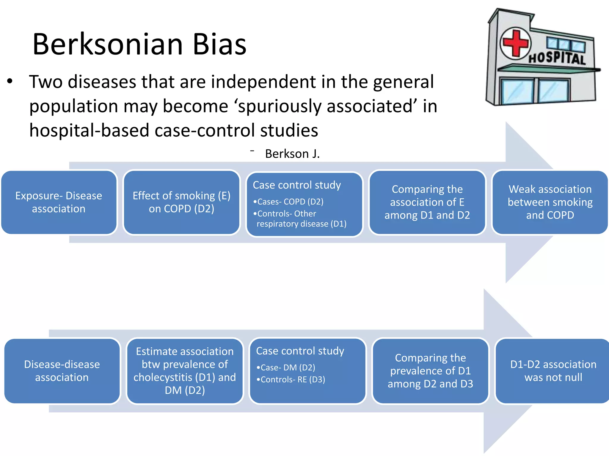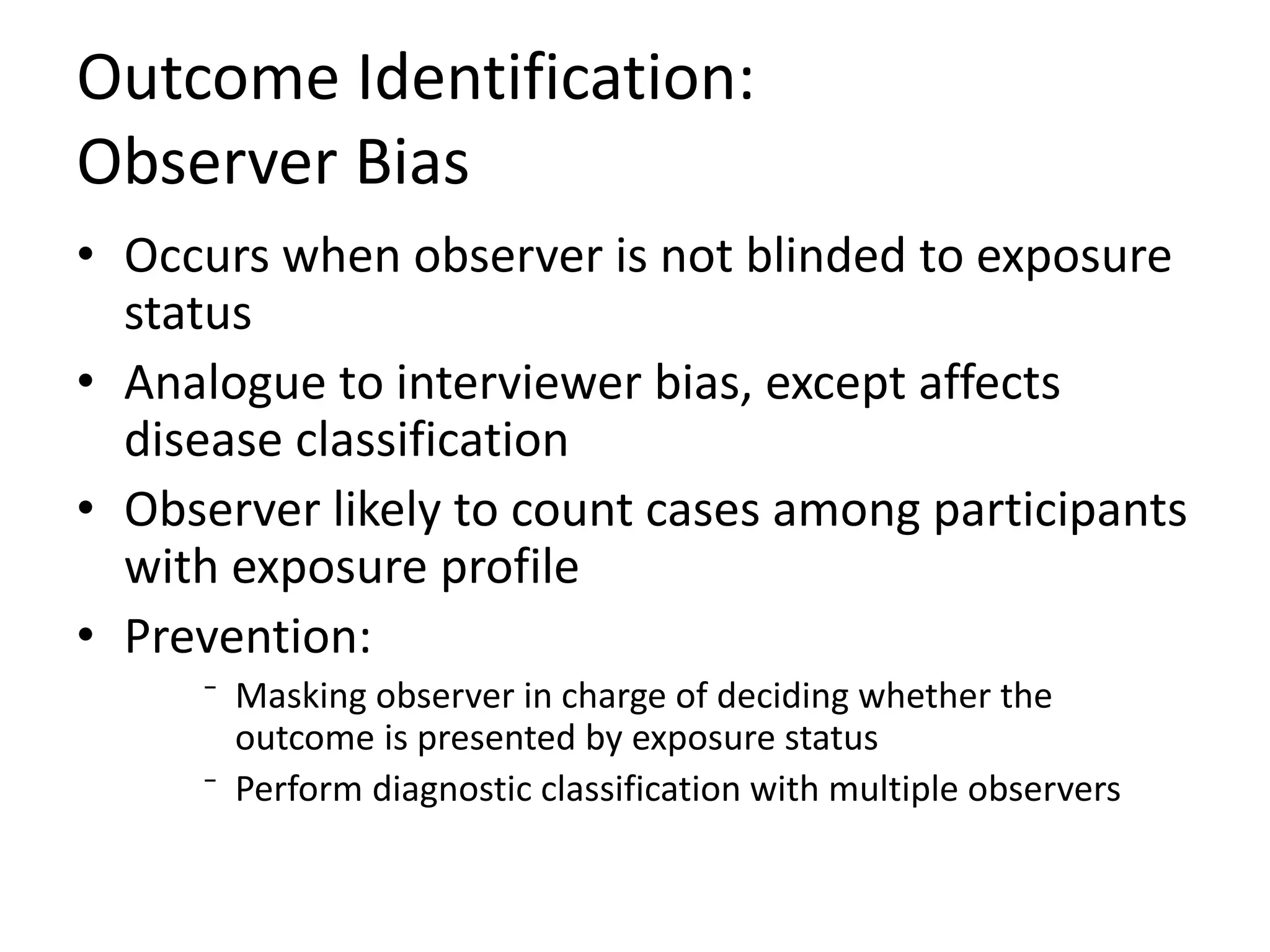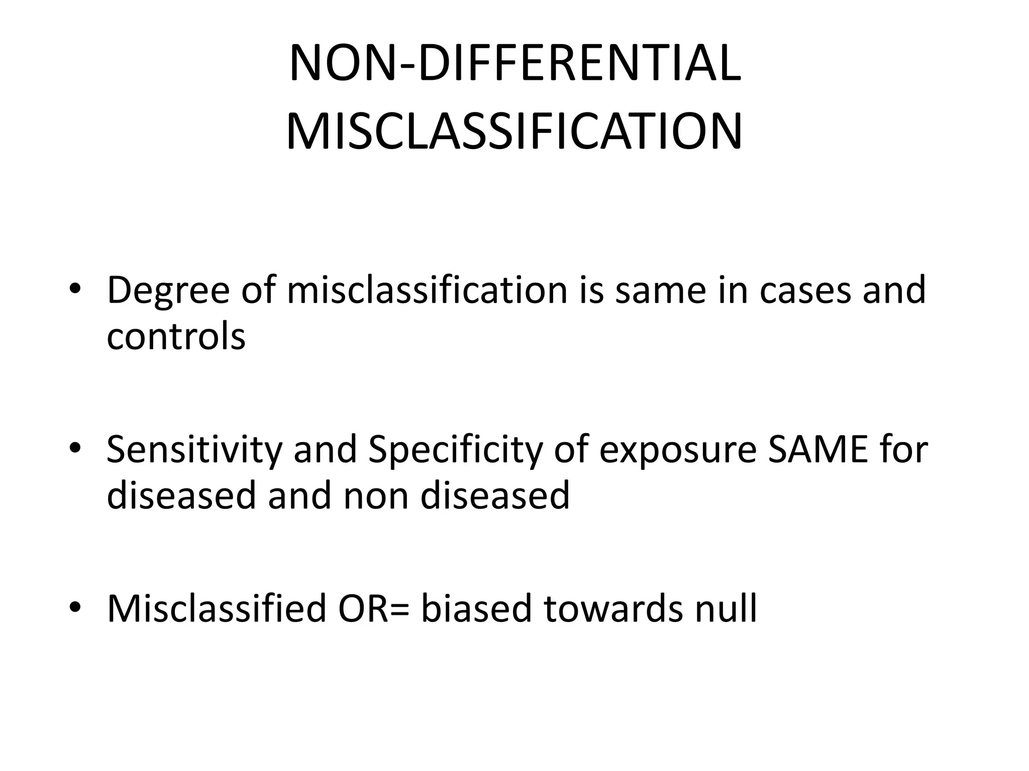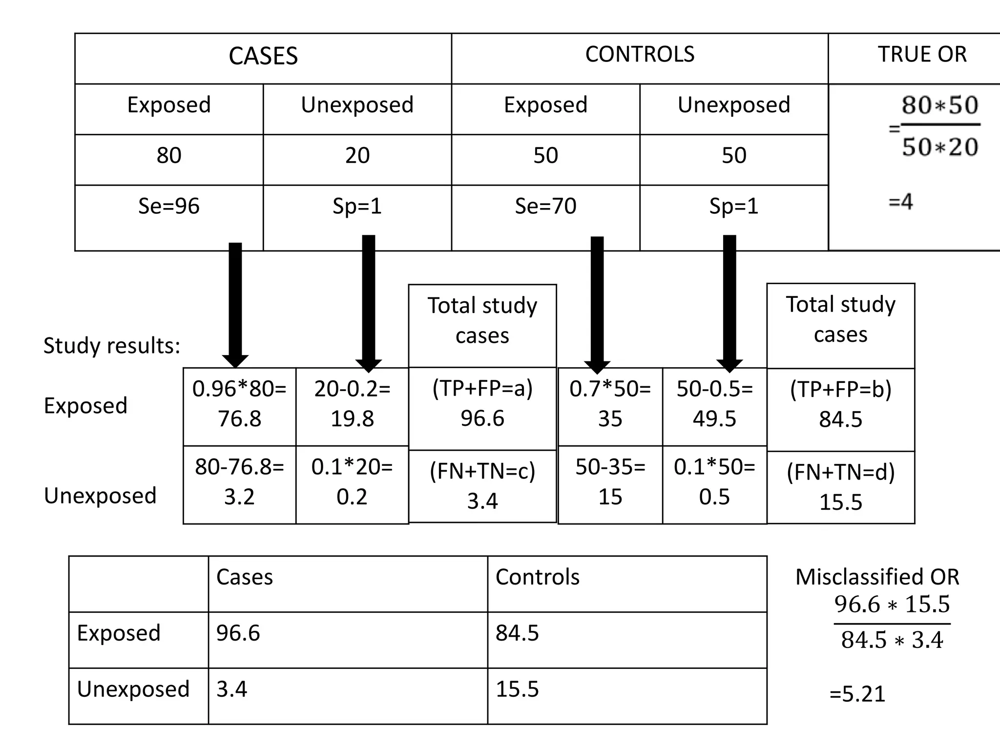2) Specific types of biases discussed include recall bias, interviewer bias, observer bias, non-response bias, inappropriate control selection, incidence-prevalence bias, loss to follow up, migration bias, Berksonian bias, healthy worker effect, exposure-related bias, non-differential misclassification, and differential misclassification. 3) Bias can

1. BIAS AND CONFOUNDER

2. Source of Association
• Casual Association- exposure causes the disease
• While causal effect may be behind an observed
association, other explanations must be
considered
• Error-‘Deviation of results from the truth’
• Random error
• Systematic error

3. RANDOM ERROR
• Average response is
exactly in the center
of the target.
• Result are valid, not
precise
SYSTEMATIC ERROR
• All the responses
missed the true
value by wide margin
• Precise, not valid
Reliable and Valid

4. RANDOM ERROR
•Due to Chance
•Effects reliability
•Tends to average out on
repeated sampling
•Reduced by increasing
the sample size or relative
size of comparison group
SYSTEMATIC ERROR
•Due to design flaw
•Effects validity
•On repeated sampling
would repeat the same
direction of error
•Avoid by careful
designing and conduct of
study

5. Systematic error
Bias
Selection Information
Exposure
Identification
Bias
Recall Bias
Interviewer Bias
Outcome
Identification
Bias
Observers Bias
Respondents
Bias
Confounder

6. BIAS
• Any systematic error in the design, conduct or
analysis of a study that results in a mistaken
estimate of an exposure’s effect on the
disease
⁻ Schlesselman JJ
• Types-
– Selection Bias
– Information Bias

7. SELECTION BIAS
• It is present when individuals have different probabilities of being included
in the study sample according to relevant study characteristics: the
exposure and the outcome of interest.
⁻ Moyses Szklo
Diseased
Exposed
Healthy
Exposed
Diseased
Unexposed
Healthy
Unexposed
Reference Population
Study Sample

8. Self selection bias
• Subjects volunteer for the study
• Volunteer induced bias
• Its possible that the subjects with desired
exposure or desired outcome may
participate more.
• Can be eliminated in RCT by randomization.
Selection
factor
Exposure Outcome
Leukemia Incidence Among Observers of a Nuclear Bomb Test
Caldwell GG et al. JAMA1980
found all observers of the Smoky Atomic test in Nevada.
In this study, 76% of the total troops were later identified and the occurrence of leukemia
was determined.
82% contacted by 18% contacted the
the investigator investigator on their own
those who contacted the investigators on their
own, i.e. self-selection - had a much higher leukemia
prevalence, over 4 times higher

9. Non Response Bias
• Due to refusals to participate in the study.
• The answers of respondents differ from the
potential answers of those who did not
answer.
• Missing data bias

10. Bias due to inappropriate control selection
• The controls selected might not be
representative of the population in which
the study was carried out
• Might have high or low level of exposure
TOTAL POPULATION
DEFINED
POPULATION
CASES CONTROLS

11. Results for tampon use as a risk factor:
OR when both control groups were combined = 29
OR when friend controls were used = 19
OR when neighbourhood controls were used = 48
If cases and controls share similar exposures (e.g. friend controls), then a and b will
tend to be nearly the same --this will bias the OR towards 1 (towards null)

12. Incidence prevalence bias
Incident cases
Wait for new cases to be diagnosed
Risk factor related to development of
the disease
Excluding patients who dies before the
diagnosis was made
Prevalent cases
Large number of cases are already
available
Risk factor related to survival with the
diseased
Including more of survivors
•Survivorship/ Neyman’s bias
•Ex- case-control study to study the relation between tobacco
smoking and AMI
Smoker patients with AMI die/ reduce smoking  Cases with
reduced exposure
Under estimation of
association

13. Loss to follow up
• Bias will occur if those who adhere have a different
disease risk than those who drop out or do not adhere
• A good rule of thumb is that <5% loss leads to little bias,
while >20% poses serious threats to validity
⁻ Joseph R Dettori
• Prevention:
• Collect baseline information to track subjects- ph no, address
• When feasible, use subjects who are easier to track- doctors or
nurses or other professionals
• Maintain regular contact via personal contact, mail, phone, or email.
• Send participants newsletters periodically to keep them updated on
the study' progress.
• Send multiple requests to non-responders.

14. Migration Bias
• When patients in one group leave their original
group, dropping out of the study altogether or
moving to one of the other groups under study
⁻ Fletcher
• Bias due to crossover more often a problem in
risk studies, than in prognosis studies, because
risk studies go on for many years
Exposed
Non
exposed

16. Berksonian Bias
• Two diseases that are independent in the general
population may become ‘spuriously associated’ in
hospital-based case-control studies
⁻ Berkson J.
Disease-disease
association
Estimate association
btw prevalence of
cholecystitis (D1) and
DM (D2)
Case control study
•Case- DM (D2)
•Controls- RE (D3)
Comparing the
prevalence of D1
among D2 and D3
D1-D2 association
was not null
Exposure- Disease
association
Effect of smoking (E)
on COPD (D2)
Case control study
•Cases- COPD (D2)
•Controls- Other
respiratory disease (D1)
Comparing the
association of E
among D1 and D2
Weak association
between smoking
and COPD

17. Healthy worker effect
• Cohort studies of occupational exposures when the
general population is used as the comparison group
• A phenomenon observed in studies of occupational
diseases: workers usually exhibit lower overall death
rates than the general population, because the severely
ill and chronically disabled are ordinarily excluded from
employment
Last J. A Dictionary of Epidemiology. 3rd ed. Oxford, UK: Oxford University Press; 1995
• Prevention:
use internal comparison groups
use external work comparison groups

18. Exposure related bias
• When investigator apply different eligibility criteria to cases
and to controls
• Exclusion bias
• Ex-association b/w reserpine and breast cancer in women
– Cases: Women with breast cancer(resperpine)
– Controls: Women without breast cancer who were not
suffering from any cardio-vascular disease
– Result: Controls likely to be on reserpine systematically
excluded  association between reserpine and breast
cancer observed
• Avoid- the inclusion and exclusion criteria should be same for
both cases and control

19. INFORMATION BIAS
• Systematic tendency for individuals selected for inclusion in the
study to be erroneously placed in different exposure or outcome
categories
• Misclassification bias
Diseased
Exposed
Healthy
Exposed
Diseased
Unexposed
Healthy
Unexposed
Reference Population
Study Sample
Cases Controls

20. Exposure Identification:
Recall Bias
• Participants are asked about past exposure
after the outcome in question has occurred as
often happens in case-control studies
• Errors in recall leads to misclassification of
exposure status
• Prevention:
⁻ Verification of exposure information
⁻ Objective markers of exposure
⁻ Nested case control or case cohort studies

21. Exposure Identification:
Interviewer Bias
• Occurs when the interviewers are not blinded
to participants disease status
• Probe differently, emphasizing certain words
to cases but not to controls
• Prevention-
• Masking/blinding of interviewers
• Careful design and conduct of quality assurance
• Training of staff
• Standardization of data collection procedures
• Monitoring of data collection activities

22. Outcome Identification:
Observer Bias
• Occurs when observer is not blinded to exposure
status
• Analogue to interviewer bias, except affects
disease classification
• Observer likely to count cases among participants
with exposure profile
• Prevention:
⁻ Masking observer in charge of deciding whether the
outcome is presented by exposure status
⁻ Perform diagnostic classification with multiple observers

23. Outcome Identification:
Respondents bias
• Participants with high risk/exposure profiles
may be more likely to report the outcome of
interest
• Prevention:
⁻ Use more of objective means
⁻ Detailed information
⁻ Confirm from hospital records

24. Result of Information Bias:
Misclassification
• There are two types of misclassification:
• Non differential misclassification
• Differential misclassification
• Definition of these terms depend on the
variable being measured i.e., exposure or
outcome

25. Diseased Non-Diseased
Exposed 80 50
Unexposed 20 50
OR =
𝑎𝑑
𝑏𝑐
=
80∗50
50∗20
=4

26. CASES CONTROLS TRUE OR
Exposed Unexposed Exposed Unexposed
=
80∗50
50∗20
=480 20 50 50
Study results:
Exposed
Unexposed
Total study
cases
TP+FP=a
FN+TN=c
TP FP
FN TN
TP FP
FN TN
Total study
cases
TP+FP=b
FN+TN=d
Se Sp Se Sp

27. CASES CONTROLS TRUE OR
Exposed Unexposed Exposed Unexposed
=
80∗50
50∗20
=4
80 20 50 50
Se=90 Sp=80 Se=90 Sp=80
Study results:
Exposed
Unexposed
Total study
cases
(TP+FP=a)
72+4=76
(FN+TN=c)
8+16=24
0.9*80
=
72
20-16=
4
80-72=
8
0.8*20
=
16
0.9*50
=
45
50-40=
10
50-45=
5
0.8*50
=
40
Total study
cases
(TP+FP=b)
50
(FN+TN=d)
45
Cases Controls
Exposed 76 50
Unexposed 24 45
Misclassified OR
76 ∗ 45
24 ∗ 55
=2.6

28. NON-DIFFERENTIAL
MISCLASSIFICATION
• Degree of misclassification is same in cases and
controls
• Sensitivity and Specificity of exposure SAME for
diseased and non diseased
• Misclassified OR= biased towards null

29. CASES CONTROLS TRUE OR
Exposed Unexposed Exposed Unexposed
80 20 50 50
Se=96 Sp=1 Se=70 Sp=1
Study results:
Exposed
Unexposed
Total study
cases
(TP+FP=a)
96.6
(FN+TN=c)
3.4
0.96*80=
76.8
20-0.2=
19.8
80-76.8=
3.2
0.1*20=
0.2
0.7*50=
35
50-0.5=
49.5
50-35=
15
0.1*50=
0.5
Total study
cases
(TP+FP=b)
84.5
(FN+TN=d)
15.5
Cases Controls
Exposed 96.6 84.5
Unexposed 3.4 15.5
Misclassified OR
96.6 ∗ 15.5
84.5 ∗ 3.4
=5.21

30. DIFFERENTIAL
MISCLASSIFICATION
• Degree of misclassification is NOT same in
cases and controls
• Sensitivity and Specificity of exposure NOT
SAME for diseased and non diseased
• Misclassified OR= biased towards null OR
away from null

31. Lead Time Bias
Patient A
Patient B
Biological
Onset
Biological
Onset
Early
Diagnosis
Diagnosis based
on Symptoms
Death
Death
Lead time
Survival

32. Publication Bias
• There are factors which dictate acceptability for
publication:
direction of finding
Tendency to publish positive results
Reluctance to accept negative results
Source of support
Language
• Absence of significant results or direction of
finding should not be used as criteria for rejection
or acceptance

33. 33
Confounding

34. • Ice cream consumption Is
higher in June, July, and
August than other months
• The death rate is higher in
June, July, and August than
other months
• Does eating ice cream cause
death?
Heat
Death
Ice cream consumption
CONFOUNDING
DEFINITION: A third variable (not the exposure or
outcome variable of interest) related to both
exposure and outcome that distorts the
observed relationship between the exposure and
outcome.
• Age is a very common source of confounding.

35. CRITERIA FOR A CONFOUNDING
FACTOR:
1. Must be a risk factor (or protective factor) for the
disease of interest.
2. Must be associated with the exposure of interest
(e.g. unevenly distributed between the exposure
groups).
3. Must not be an intermediate step in the causal
pathway between the exposure and outcome

36. Physical
inactivity
Heart Disease
AG
E
Fluid
intake
?
if the age distribution is similar in the exposure groups being compared,
then age will not cause confounding.
Direction of Confounding
• Confounding “pulls” the observed association away
from the true association
– It can either exaggerate/over-estimate the true
association (positive confounding)
• Example
– ORcausal = 1.0
– ORobserved = 3.0
or
– It can hide/under-estimate the true association (negative
confounding)
• Example
– ORcausal = 3.0
– ORobserved = 1.0

37. Bias and Confounding
Bias creates an association that is not
true, but confounding describes an
association that is true, but potentially
misleading.

38. Control of confounding
• Control at the design stage
– Randomization
– Restriction
– Matching
• Control at the analysis stage
– Conventional approaches
• Stratified analyses
• Multivariate analyses

39. Randomization
– for intervention studies
– Definition: random assignment of study
subjects to exposure categories
– To control/reduce the effect of confounding
variables about which the investigator is
unaware (i.e. both known and unknown
confounders get distributed evenly because
of randomization)
– Randomization does not always eliminate
confounding

40. Restriction
• restrict study subjects to only those falling with specific level(s)
of a confounding variable
• E.g. study of alcohol and MI may exclude smokers since
smoking is an important confounder
• in the hypothetical study looking at the association between
physical activity and heart disease, suppose that age and gender
were the only two confounders of concern. If so, confounding by
these factors could have been avoided by making sure that all
subjects were males between the ages of 40-50. This will ensure
that the age distributions are similar in the groups being
compared, so that confounding will be minimized.
• Advantages of restriction
• straightforward, convenient, inexpensive (but, reduces recruitment!)
Disadvantages of restriction
• Disadvantages Will limit number of eligible subjects
• Will limit ability to generalize the study findings
• Residual confounding may persist if restriction categories not sufficiently narrow
(e.g. “decade of age” might be too broad)

41. • Disadvantages of matching
• Finding appropriate control subjects: difficult and expensive and limit sample size
• Confounder used to match subjects cannot be evaluated with respect to the
outcome/disease
• Matching does not control for confounders other than those used to match (Residual
confounding)
• 0vermatching
• If controls are selected to match the cases for a factor that is correlated with
exposure, this will change the distribution of the control population away from
the distribution in the source population then
• –This will introduce a selection bias that is very similar to confounding.
• –If the matching factor were perfectly correlated with the exposure, the exposure
distribution of controls would be identical to cases, and the crude OR estimate
would be 1.0
Matching
• Matching is commonly used in case-control studies
• Match on strong confounder
• Types:
– Pair (individual) matching
– Frequency matching
• The use of matching usually requires special analysis techniques (e.g.
matched pair analyses and conditional logistic regression)

42. 42
Matched pair analysis
a B
c d
case
Not exposed
exposed
exposed Not exposed
control
Matched pair analysis
• concordant pairs do not contribute to our knowledge as they do not
differ in terms of exposure status
• For discordant pairs
the odds ratio simplifies to
Number of discordant pairs with case exposed/Number of discordant pairs with control
exposed
=b/c

43. 43
Matched pair analysis
Odds ratio = 5/4 = 1.25
Case control
1 0
1 1
1 0
1 0
0 0
1 0
1 1
0 1
0 0
0 1
0 1
0 0
1 0
0 1
Cases and control were matched for potential
confounder
1= exposure present
0 = exposure absent
2 5
4 3
exposed
Not exposed
case
control
exposed Not exposed

44. Control of confounding at analysis
stage
•Stratification
• Objective of stratified analysis is to “fix” the level of the confounding
variable and produce groups within which the confounder does not
vary
• Then evaluate the exposure-disease association within each stratum
of the confounder
• Within each stratum, the confounder cannot confound because it
does not vary

45. Hypothesis:High alcohol consumption is associated with
stomach cancer (case-control study)
D+ D-
E+ 62 35 97
E- 68 95 163
130 130 260
Crude OR = 2.47

46. D+ D-
E+ 18 20 38
E- 42 80 122
60 100 160
NON-SMOKERS SMOKERS
D+ D-
E+ 44 15 59
E- 26 15 41
70 30 100
OR = 1.71 OR = 1.69
Is there evidence that smoking confounds
the relationship between alcohol
consumption and stomach cancer?

47. In general:
If Strata 1 OR, Strata 2 OR < Crude OR
or
If Strata 1 OR, Strata 2 OR > Crude OR
then confounding is present.
CRUDE
ORCA = 2.47
STRATA 1
ORNS = 1.71
STRATA 2
ORSM = 1.69
A more direct way to evaluate confounding is to
aggregate the strata-specific point estimates to
obtain a standardized (adjusted) estimate
Maentel Hanzel method is used to adjust for smoking and produce an
adjusted odds ratio =1.7

48. Crude 2 x 2 table
Calculate Crude OR (or RR)
Stratify by Confounder
Calculate OR’s
for each stratum
calculate adjusted OR (e.g. MH)
Crude
Stratum 1 Stratum 2
If Crude OR =/= Adjusted OR,
confounding is likely
If Crude OR = Adjusted
OR, confounding is unlikely
ORCrude
OR1 OR2
Stratified Analysis
OR1, OR2 < ORCrude
OR1, OR2 > ORCrude

49. Crude: does not take into account the effect of the confounder
Adjusted: accounts for the confounder
Mantel-Haenszel method estimator
Multivariate analyses (e.g. logistic regression)
The magnitude of confounding is assessed by looking at the discrepancy between the
crude and adjusted estimates

50. 50
Mantel-Haenszel Confounder-adjusted Odds Ratio
a1 b1
c1 d1
T1
a2 b2 a b
c2 d2 c d
T2 T
a3 b3
c3 d3
T3
etc.
CRUDE odds-ratio=ad/bc = (ai)(di)/(bi)(ci),
where the summations are over all strata.
Mantel-Haenszel adjusted odds-ratio=(aidi/Ti)/( bici/Ti),
where the summations are also over all strata.
Mantel-Haenszel adjusted odds-ratio=(aidi/Ti)/( bici/Ti),
= (a1d1/T1)+(a2d2/T2)+(a3d3/T3) + etc
divided by
(b1c1/T1)+(b2c2/T2)+ (b3c3/T3) + etc

51. 51
Mantel-Haenszel Analysis
Lung cancer
Present
Lung cancer
Absent
Total 300 300
Drinks alcohol 210 120
Does not drink 90 180
Crude OR = (210  180)/(120 90) = 3.5
Hypothetical Case-Control Study with Confounding
Smokers
Disease
Present
Disease
Absent
Total
Total 245 96 341
Exposed 197 77
Unexposed 48 19
OR FOR SMOKERS = (197X19)/(77X48)=12500/500=1.01
Non-smokers
Disease
Present
Disease
Absent
Total
Total 55 204 259
Exposed 13 43
Unexposed 42 161
OR FOR NON-SMOKERS = (13X161)/(43X42)=1.18
Mantel-Haenszel OR = 197x19/341+13x161/259 = 1.06
77X48/341+43x42/259

52. Multivariate Analysis
• Stratified analysis works best only in the presence of 1 or 2 confounders
• If the number of potential confounders is large, multivariate analyses offer the
only real solution
• Can handle large numbers of confounders (covariates) simultaneously
• Based on statistical regression “models”
• E.g. logistic regression, multiple linear regression
• Always done with statistical software packages

53. • Residual confounding
• Confounding can persist, even after adjustment
• Why?All confounders were not adjusted for (unmeasured
confounding)
• Some variables were actually not confounders!
• Confounders were measured with error (misclassification of
confounders)
• Categories of the confounding variable are improperly defined
(e.g. age categories were too broad)
“Whichever method you choose, you have to
know potential confounders reported in
previous studies.”
Literature searching is important

54. Effect modification
What not is Confounding
• Confounding IS NOT
• A factor that modifies the relationship between an exposure and a disease
Effect of exposure on the disease is modified depending on the value of a
third variable:
the “effect modifier”
Exposure Disease
Effect modifier
Effect modification/interaction
Two definitions (related):
 Based on homogeneity or heterogeneity of effects
 Interaction occurs when the effect of a risk factor (X) on an outcome (Y) is not homogeneous in strata
formed by a third variable (Z, effect modifier)
 Based on the comparison between observed and expected joint effects of a risk factor
and a third variable
 Interaction occurs when the observed joint effects of the risk factor (X) and third variable (Z) differs
from that expected on the basis of their independent effects

55. Effect Modification(aka Interaction)
Hospitalized Not Hospitalized Total
Male 1330 7018 8348
Female 798 6400 7198
Hospitalize
d
Not
Hospitalize
d
Total
Male 966 3146 4112
Female 460 3000 3450
Hospitalize
d
Not
Hospitalize
d
Total
Male 364 3872 4236
Female 348 3400 3748
Crude risk ratio=1.44
Age <40 Age >40
Stratum-specific risk
ratio=1.80
Stratum-specific risk ratio=0.93

56. Crude 2 x 2 table
Calculate Crude OR (or RR)
Stratify by Confounder
Calculate OR’s
for each stratum
Crude
Stratum 1 Stratum 2
If Crude OR =/= Adjusted OR,
confounding is likely.
Report Adjusted OR
If Crude OR = Adjusted OR,
confounding is unlikely.
Report Crude OR
ORCrude
OR1 OR2
Stratified Analysis
If stratum-specific OR’s are the same
or similar, calculate adjusted OR (e.g.
MH)
If stratum-specific OR’s are not
similar,
Effect modification is present.
Report Stratum-specific OR

57. Confounding vs. interaction
 Confounding is a problem we want to
eliminate (control or adjust for) in our study
 Comparing crude vs. adjusted effect estimates
 Interaction is a natural occurrence that we
want to describe and study further
 Comparing stratum-specific estimates

58. Confounding or Effect Modification ?
Birth Weight Leukaemia
gender
Does birth weight association differ in strength according to sex?
Birth Weight Leukaemia
Birth Weight Leukaemia/ /
BOYS
GIRLS
OR = 1.8
OR = 0.9
OR = 1.5

59. • Thankyou