Download as PDF, PPTX


![Simulating the RRW: Asymptotic Variance
The CLT requires a third moment for the increments
E[∆(0)] < 0 and E[∆(0)3 ] < ∞
1
Asymptotic variance = O
(1 − ρ)4 Whitt 1989
Asmussen 1992](https://image.slidesharecdn.com/rrwsimstalk9-15-09-090917083434-phpapp02/75/Why-are-stochastic-networks-so-hard-to-simulate-12-2048.jpg)
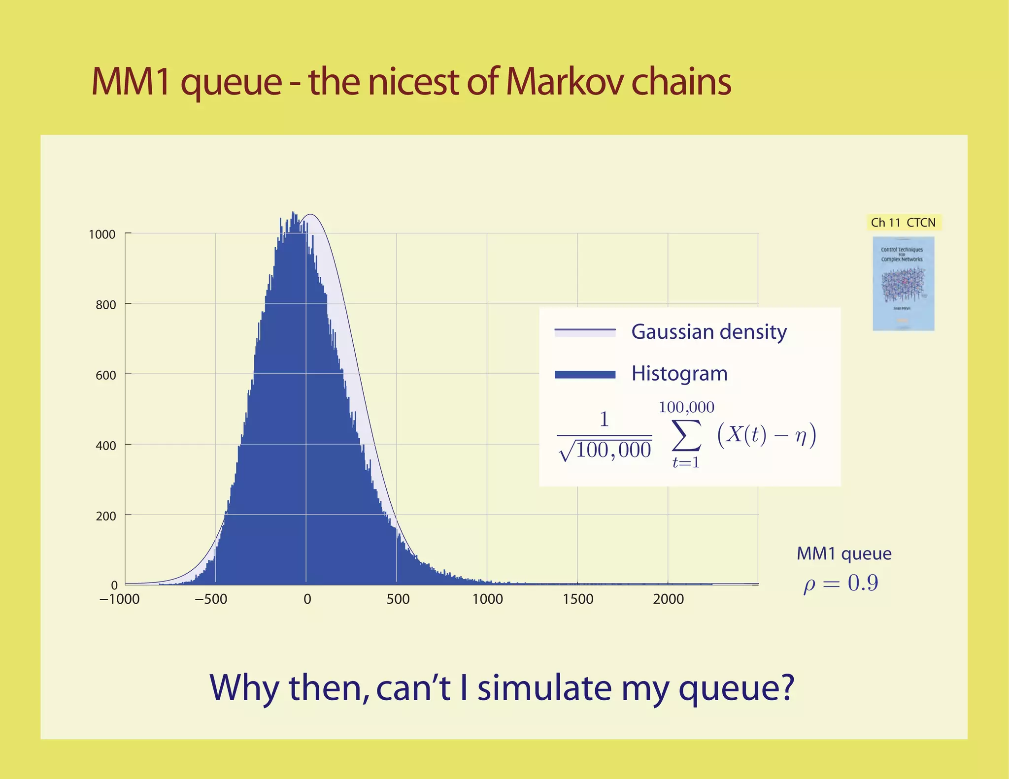
![Simulating the RRW: Asymptotic Variance
The CLT requires a third moment for the increments
E[∆(0)] < 0 and E[∆(0)3 ] < ∞
1
Asymptotic variance = O
(1 − ρ)4
Ch 11 CTCN
1000
800
Gaussian density
600 Histogram
100,000
1
400
√ X(t) − η
100,000 t=1
200
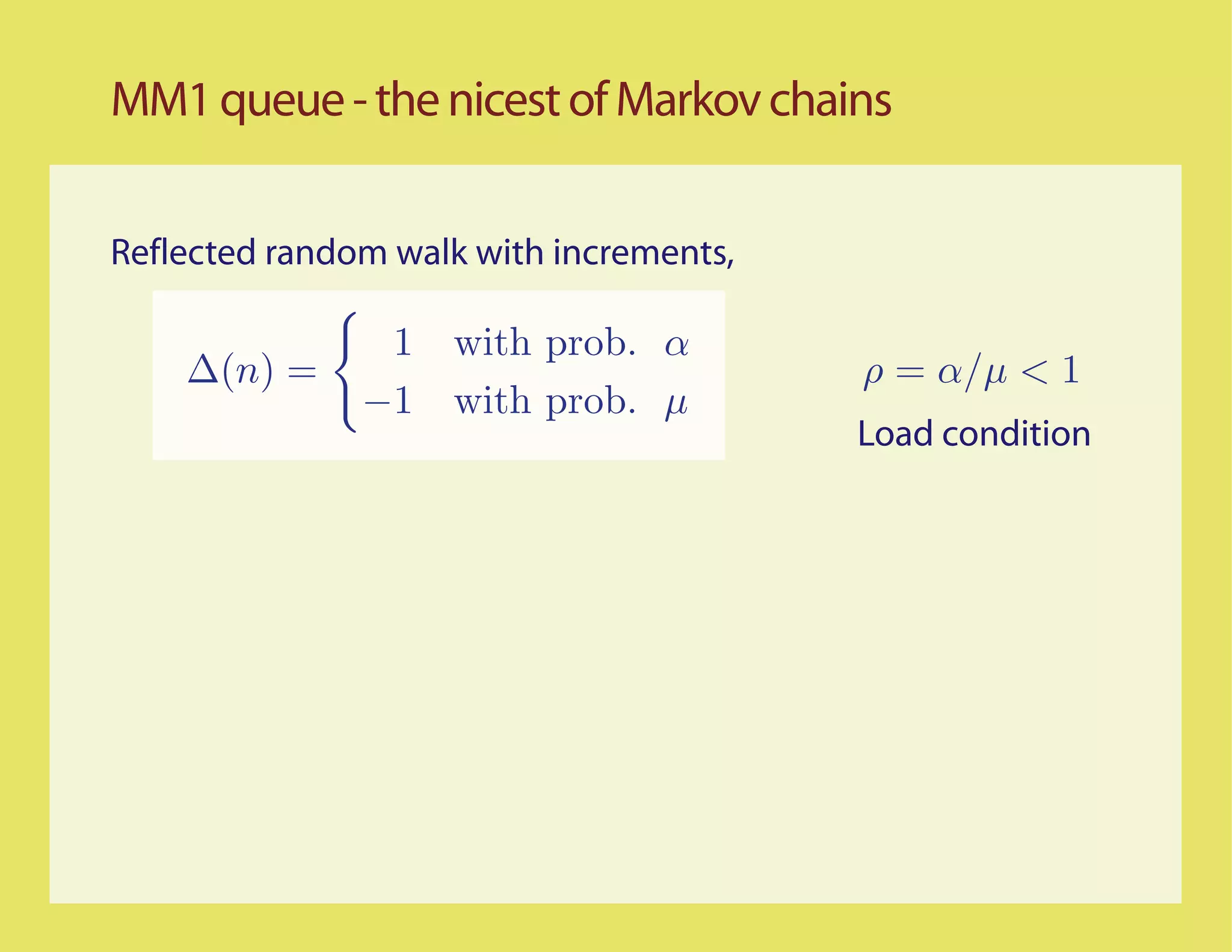
MM1 queue
0 ρ = 0.9
−1000 −500 0 500 1000 1500 2000](https://image.slidesharecdn.com/rrwsimstalk9-15-09-090917083434-phpapp02/75/Why-are-stochastic-networks-so-hard-to-simulate-13-2048.jpg)
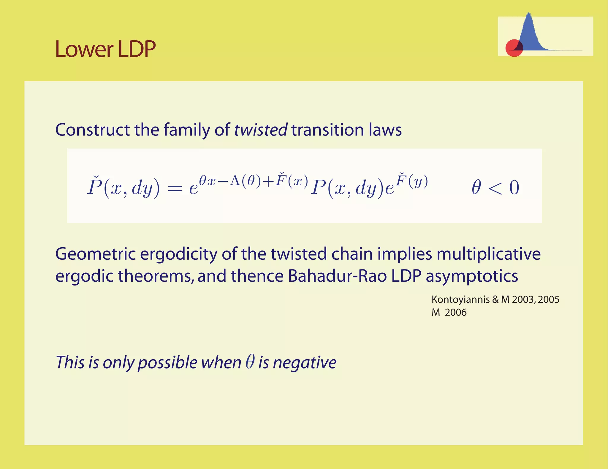
![Simulating the RRW: Lopsided Statistics
Assume only negative drift, and finite second moment:
E[∆(0)] < 0 and E[∆(0)2 ] < ∞
Lower LDP asymptotics: For each r < η ,
1
lim log P η(n) ≤ r
n→∞ n
= −I(r) < 0
M 2006](https://image.slidesharecdn.com/rrwsimstalk9-15-09-090917083434-phpapp02/75/Why-are-stochastic-networks-so-hard-to-simulate-14-2048.jpg)
![Simulating the RRW: Lopsided Statistics
Assume only negative drift, and finite second moment:
E[∆(0)] < 0 and E[∆(0)2 ] < ∞
Lower LDP asymptotics: For each r < η ,
1
lim log P η(n) ≤ r
n→∞ n
= −I(r) < 0
M 2006
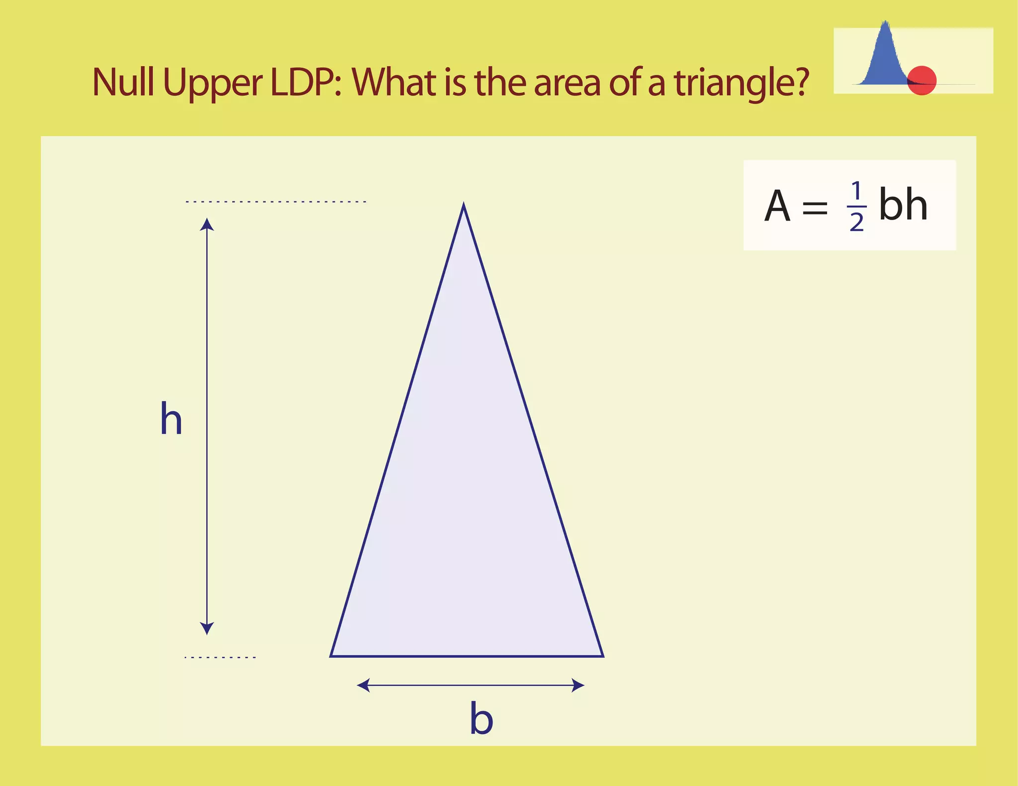
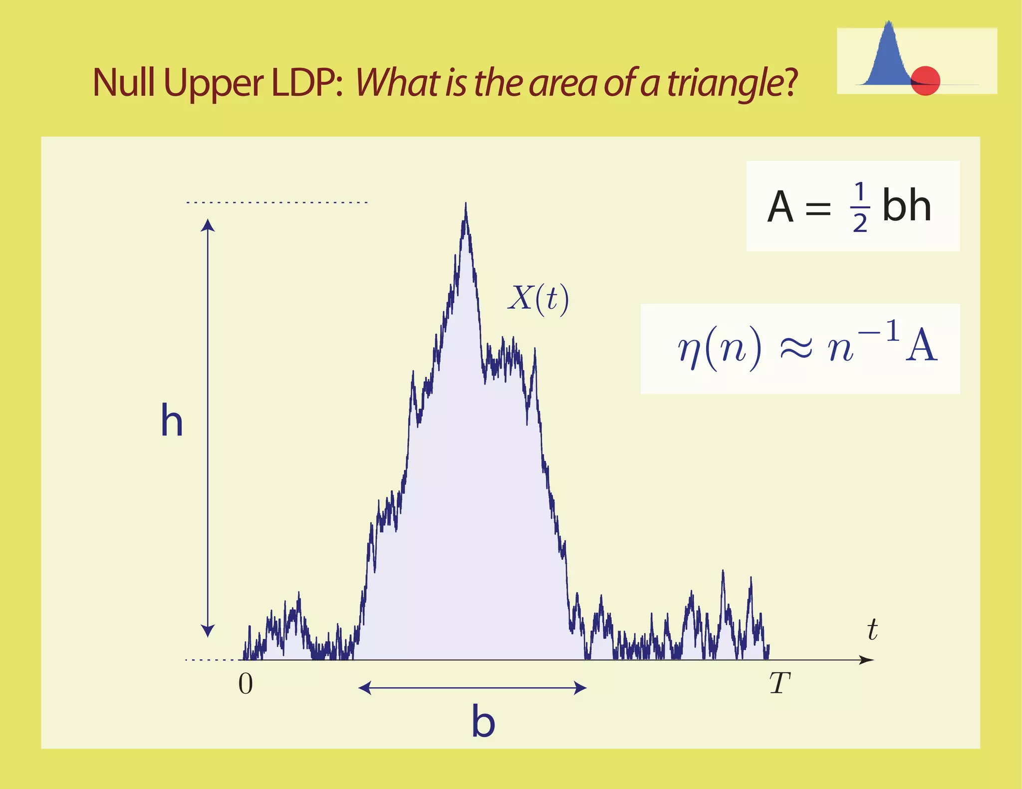
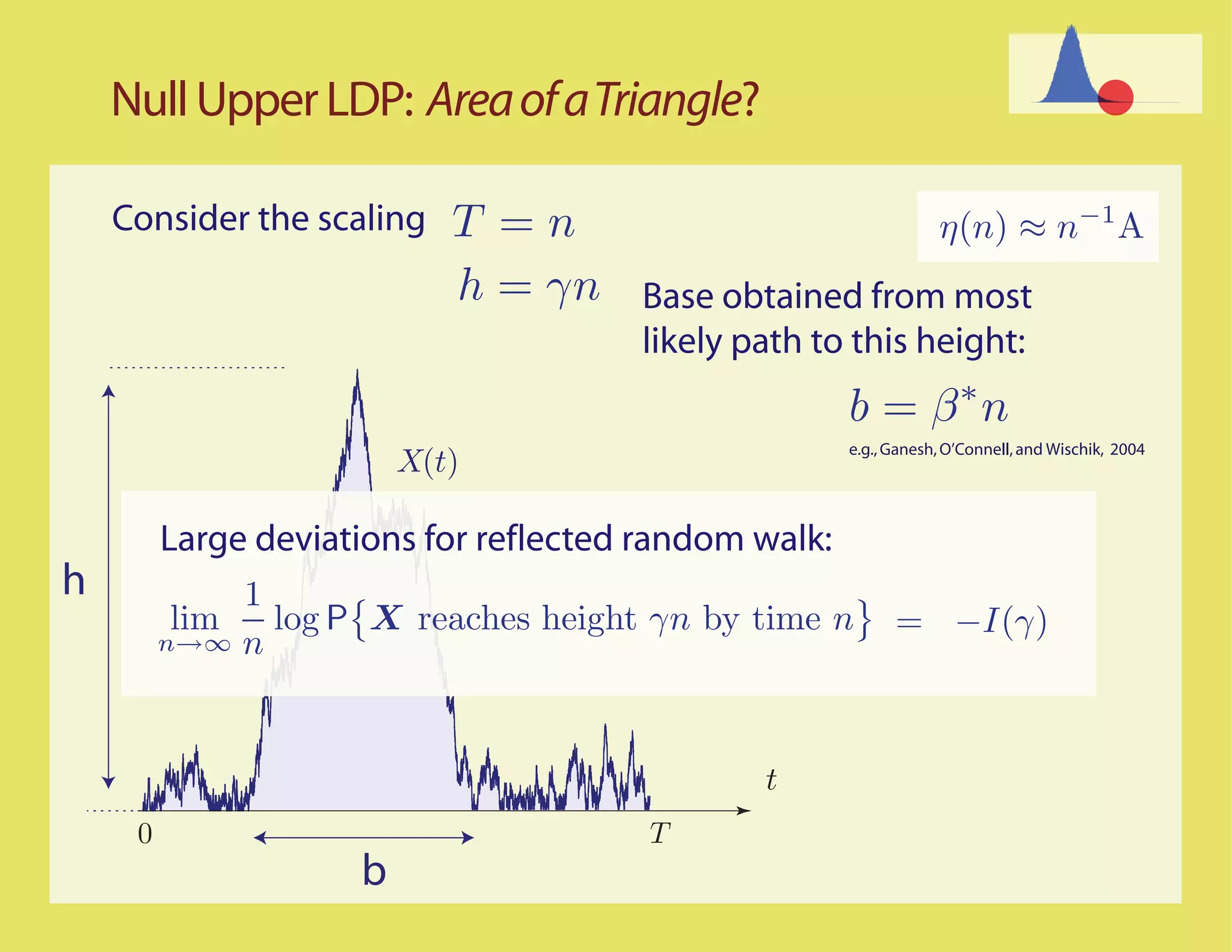
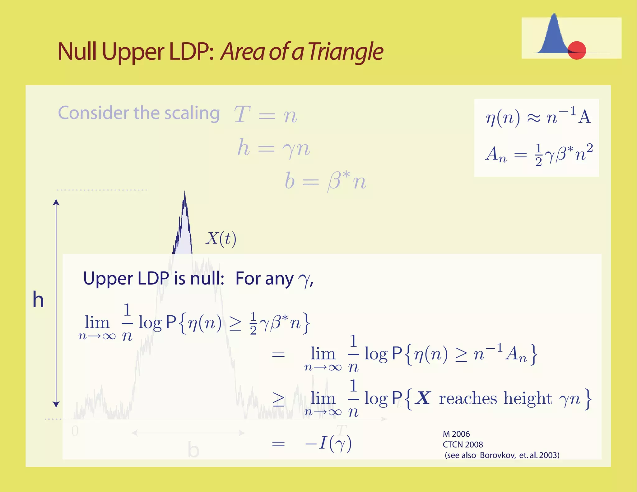
Upper LDP asymptotics are null: For each r ≥ η ,
1
lim log P η(n) ≥ r = 0 M 2006
n→∞ n CTCN
even for the MM1 queue!](https://image.slidesharecdn.com/rrwsimstalk9-15-09-090917083434-phpapp02/75/Why-are-stochastic-networks-so-hard-to-simulate-15-2048.jpg)


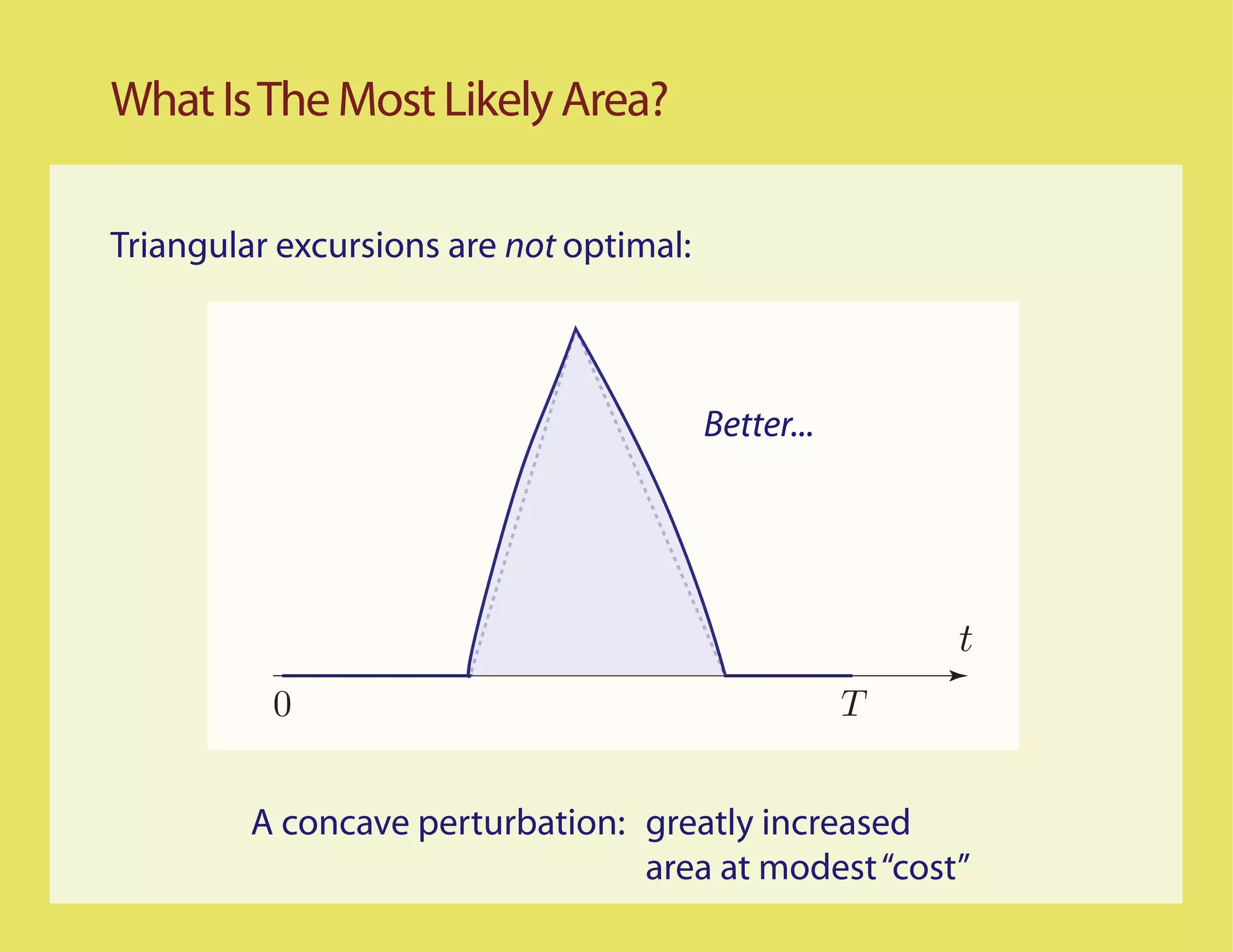
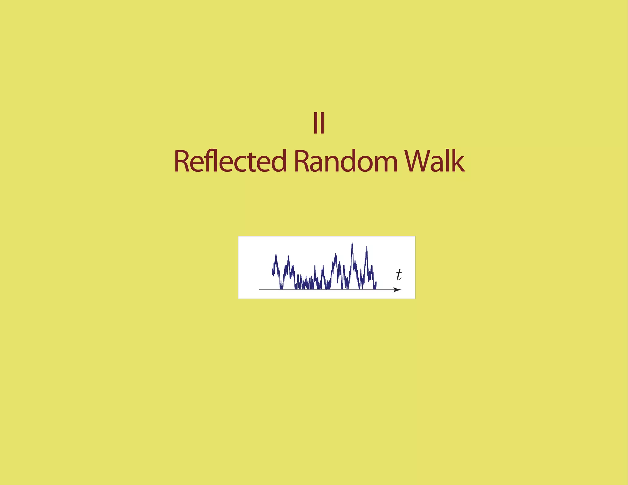
![Better...
Most Likely Paths t
0 T
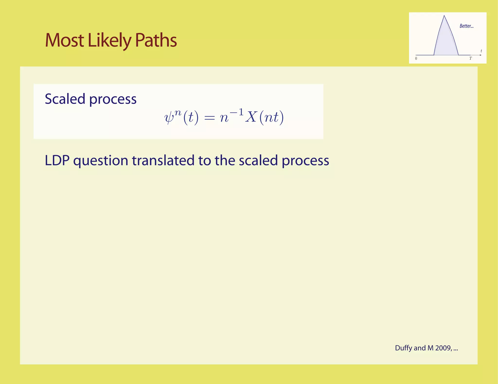
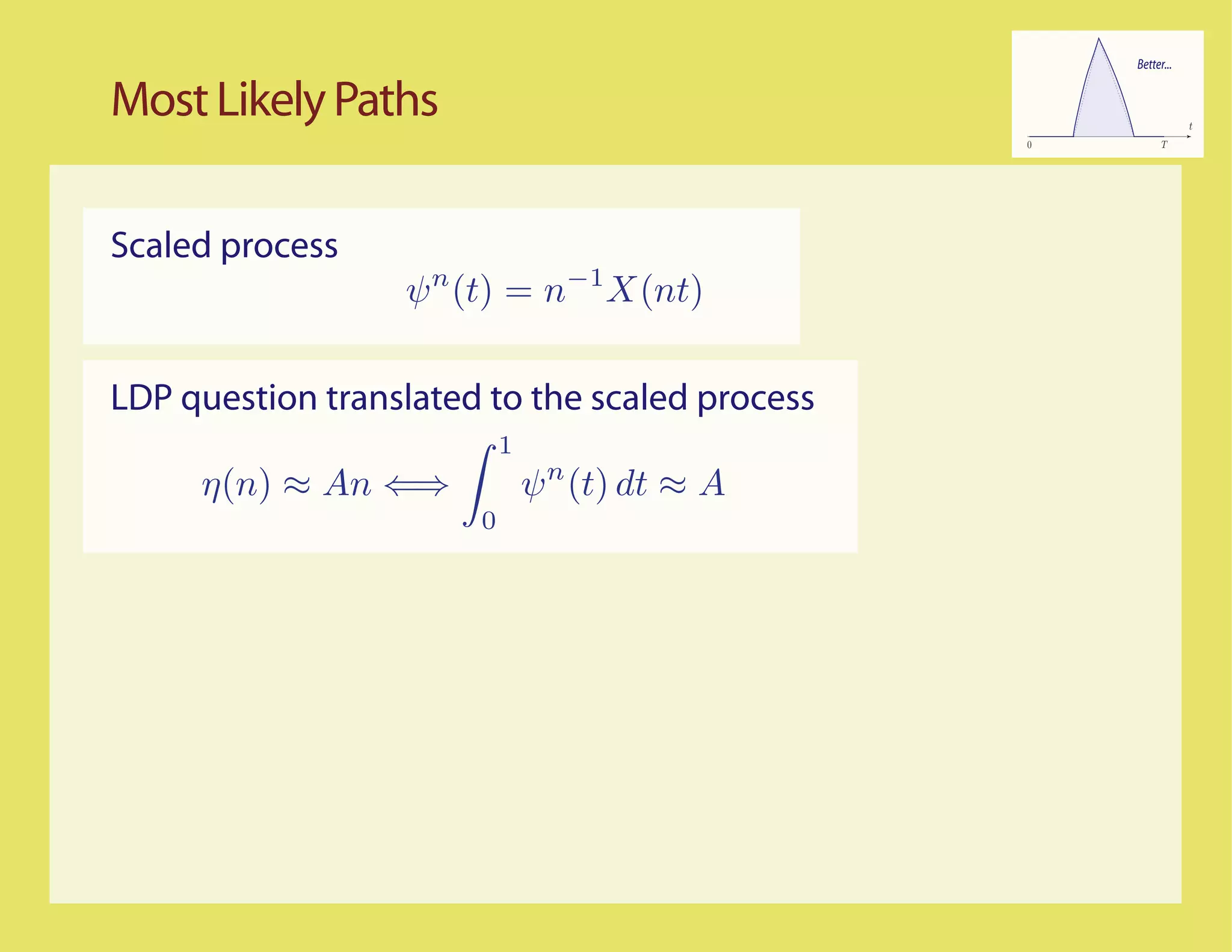
Scaled process
ψ n (t) = n−1 X(nt)
LDP question translated to the scaled process
1
η(n) ≈ An ⇐⇒ ψ n (t) dt ≈ A
0
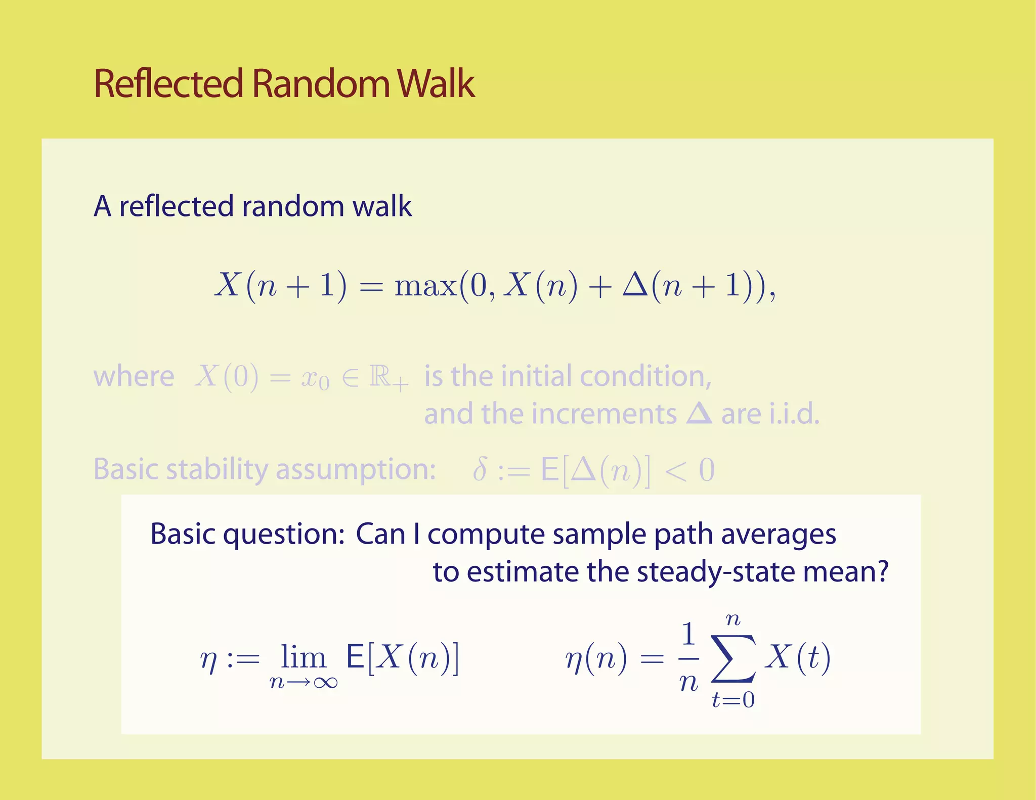
Basic assumption: The sample paths for the unconstrained
random walk with increments ∆ satisfy the LDP in D[0,1] with
good rate function IX](https://image.slidesharecdn.com/rrwsimstalk9-15-09-090917083434-phpapp02/75/Why-are-stochastic-networks-so-hard-to-simulate-29-2048.jpg)
![Better...
Most Likely Paths t
0 T
Scaled process
ψ n (t) = n−1 X(nt)
LDP question translated to the scaled process
1
η(n) ≈ An ⇐⇒ ψ n (t) dt ≈ A
0
Basic assumption: The sample paths for the unconstrained
random walk with increments ∆ satisfy the LDP in D[0,1] with
good rate function IX
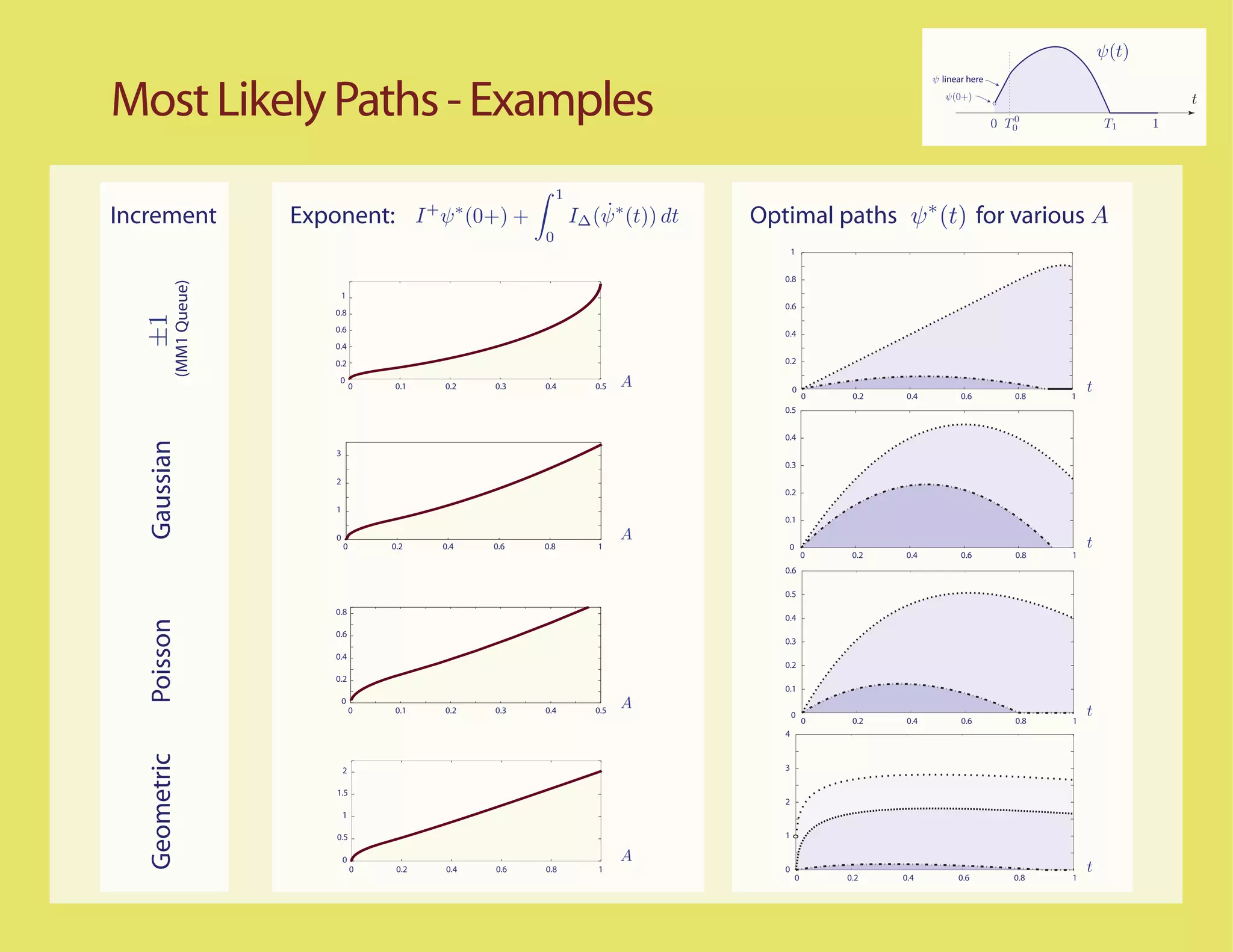
1
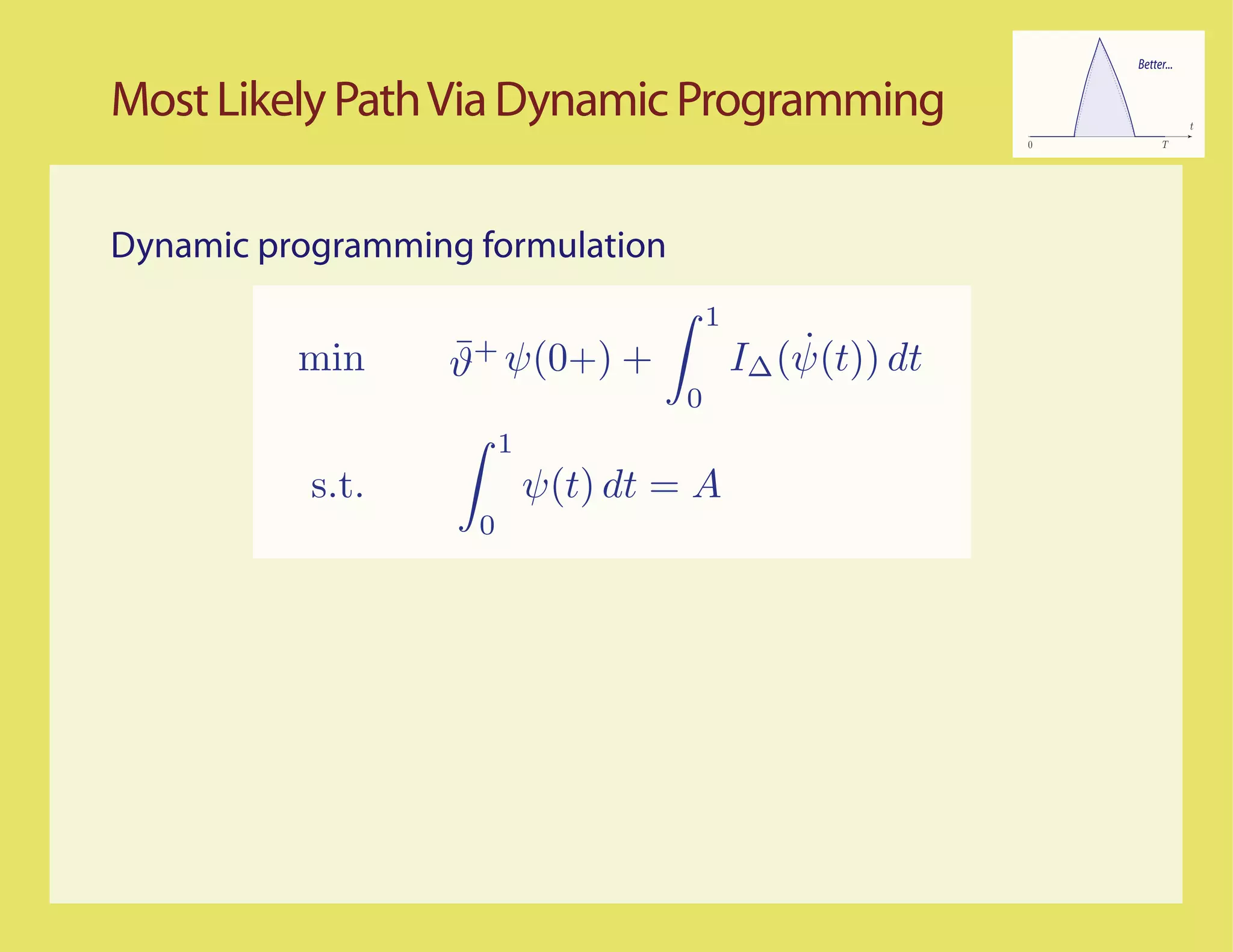
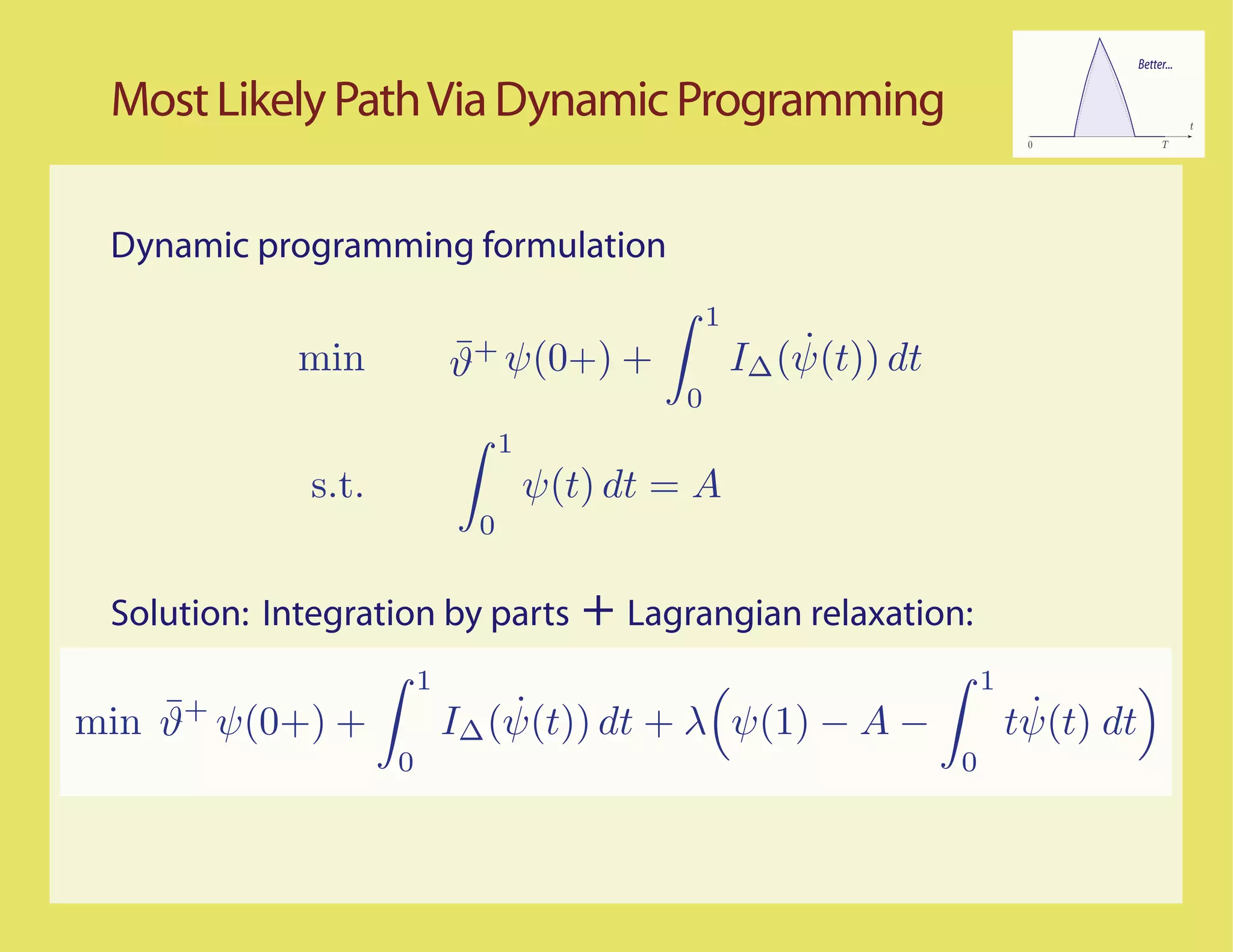
¯
IX (ψ) = ϑ+ ψ(0+) + ˙
I∆ (ψ(t)) dt For concave ψ, with
no downward jumps
0](https://image.slidesharecdn.com/rrwsimstalk9-15-09-090917083434-phpapp02/75/Why-are-stochastic-networks-so-hard-to-simulate-30-2048.jpg)


![[1] S. P. Meyn. Large deviation asymptotics and control variates for simulating large functions. Ann. Appl.
Probab., 16(1):310–339, 2006.
[2] S. P. Meyn. Control Techniques for Complex Networks. Cambridge University Press, Cambridge, 2007.
[3] K. R. Duffy and S. P. Meyn. Most likely paths to error when estimating the mean of a reflected random
walk. http://arxiv.org/abs/0906.4514, June 2009.
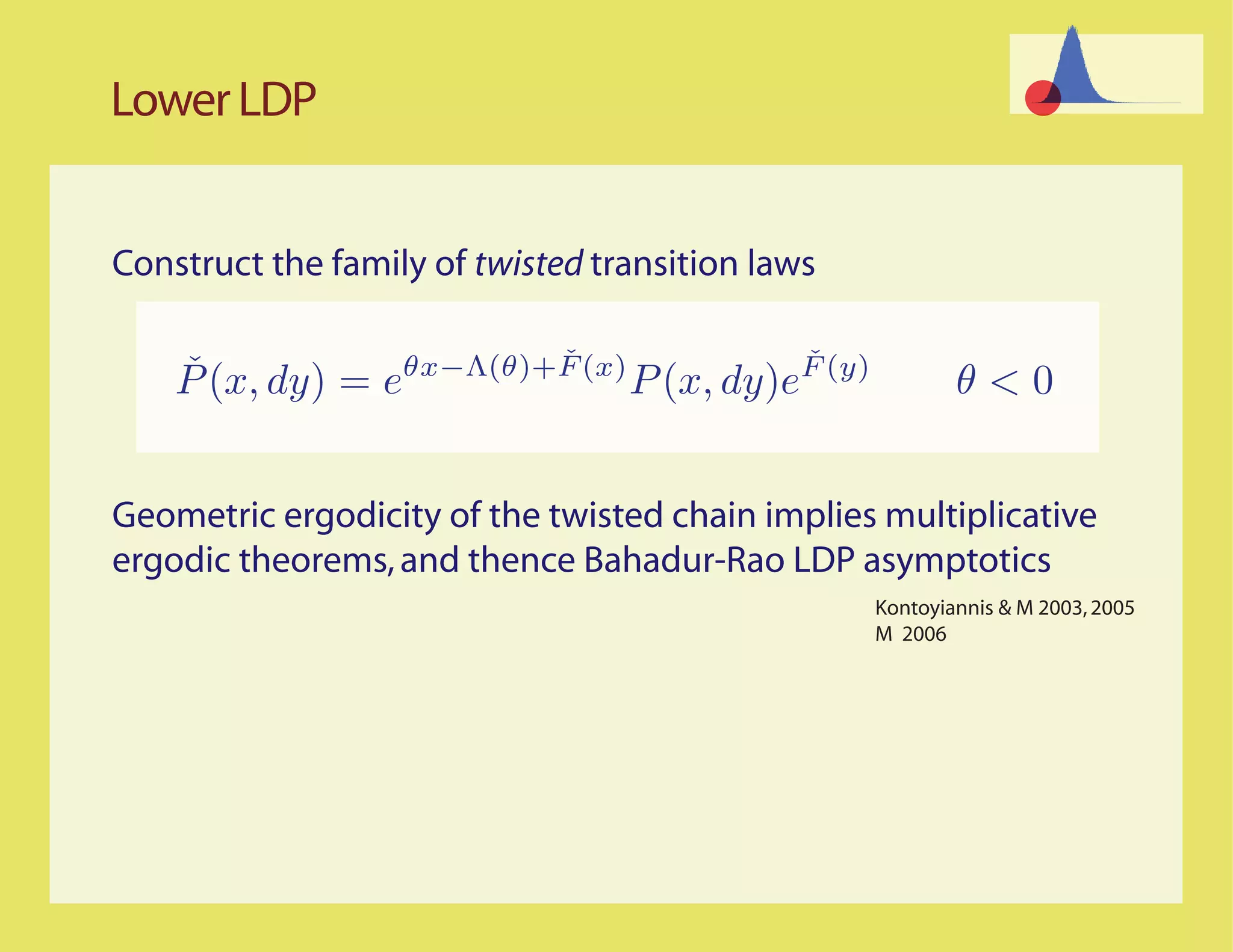
References [1] I. Kontoyiannis and S. P. Meyn. Spectral theory and limit theorems for geometrically ergodic Markov
processes. Ann. Appl. Probab., 13:304–362, 2003. Presented at the INFORMS Applied Probability
Conference, NYC, July, 2001.
[2] I. Kontoyiannis and S. P. Meyn. Large deviations asymptotics and the spectral theory of multiplicatively
regular Markov processes. Electron. J. Probab., 10(3):61–123 (electronic), 2005.
[1] G. Fort, S. Meyn, E. Moulines, and P. Priouret. ODE methods for skip-free Markov chain stability with
applications to MCMC. Ann. Appl. Probab., 18(2):664–707, 2008.
[2] V. S. Borkar and S. P. Meyn. The O.D.E. method for convergence of stochastic approximation and
reinforcement learning. SIAM J. Control Optim., 38(2):447–469, 2000.
LDPs for RRW
[1] S. P. Meyn. Large deviation asymptotics and control variates for simulating large functions. Ann. Appl.
Probab., 16(1):310–339, 2006.
[2] S. P. Meyn. Control Techniques for Complex Networks. Cambridge University Press, Cambridge, 2007.
[3] K. R. Duffy and S. P. Meyn. Most likely paths to error when estimating the mean of a reflected random
walk. http://arxiv.org/abs/0906.4514, June 2009.
Exact LDPs
[1] I. Kontoyiannis and S. P. Meyn. Spectral theory and limit theorems for geometrically ergodic Markov
processes. Ann. Appl. Probab., 13:304–362, 2003.
[2] I. Kontoyiannis and S. P. Meyn. Large deviations asymptotics and the spectral theory of multiplicatively
regular Markov processes. Electron. J. Probab., 10(3):61–123 (electronic), 2005.
Simulation
[1] S. G. Henderson, S. P. Meyn, and V. B. Tadi´. Performance evaluation and policy selection in multiclass
c
networks. Discrete Event Dynamic Systems: Theory and Applications, 13(1-2):149–189, 2003. Special
issue on learning, optimization and decision making (invited).
[2] S. P. Meyn. Control Techniques for Complex Networks. Cambridge University Press, Cambridge, 2007.
[1] G. Fort, S. Meyn, E. Moulines, and P. Priouret. ODE methods for skip-free Markov chain stability with
applications to MCMC. Ann. Appl. Probab., 18(2):664–707, 2008.
[2] V. S. Borkar and S. P. Meyn. The ODE method for convergence of stochastic approximation and
reinforcement learning. SIAM J. Control Optim., 38(2):447–469, 2000.](https://image.slidesharecdn.com/rrwsimstalk9-15-09-090917083434-phpapp02/75/Why-are-stochastic-networks-so-hard-to-simulate-46-2048.jpg)

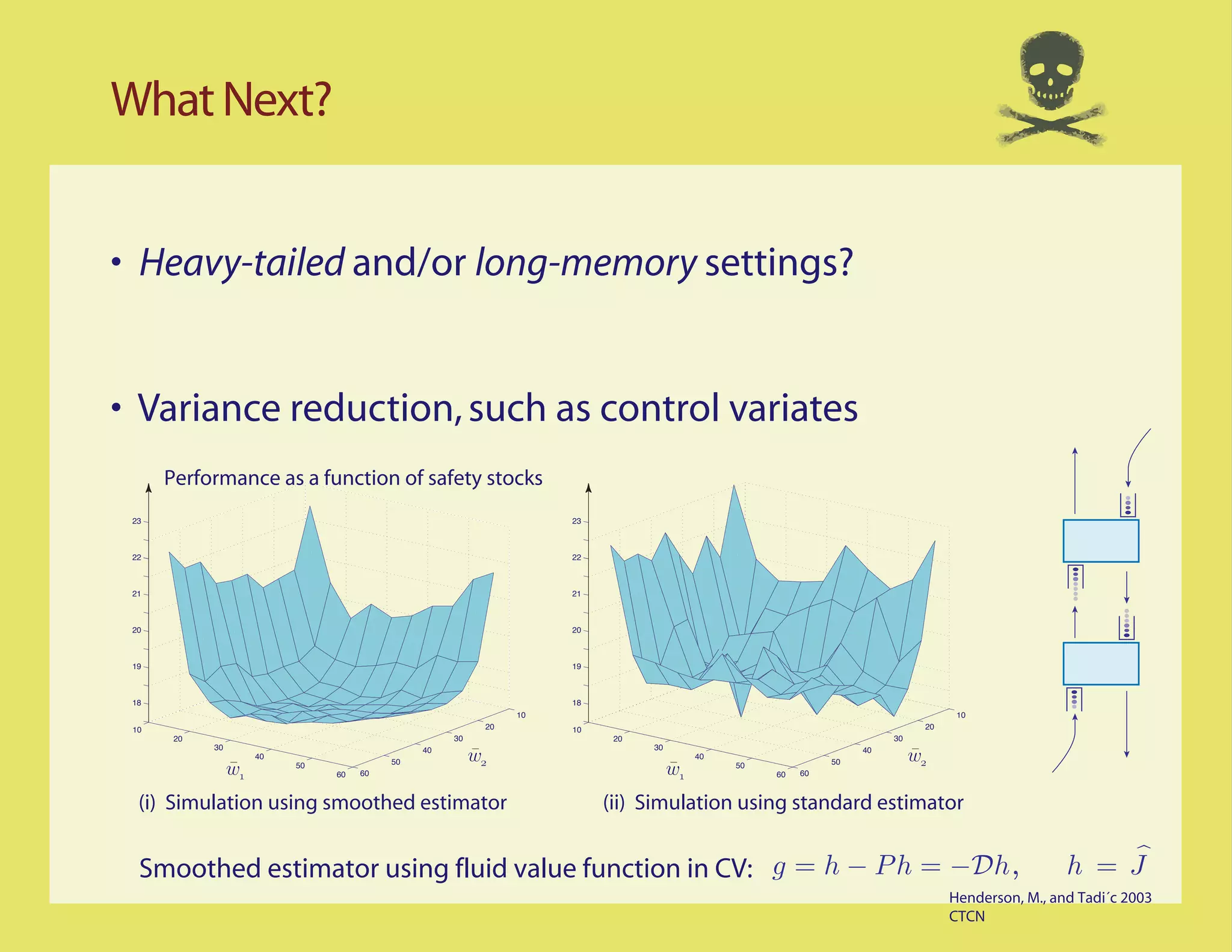
The document discusses the challenges of simulating reflected random walks (RRW) and the implications for queueing models, particularly the MM1 queue. It highlights the high variance in simulations during 'heavy traffic' and presents findings on sample-path behavior under large deviations. The document also suggests future research directions, including examining heavy-tailed or long-memory settings and variance reduction techniques.