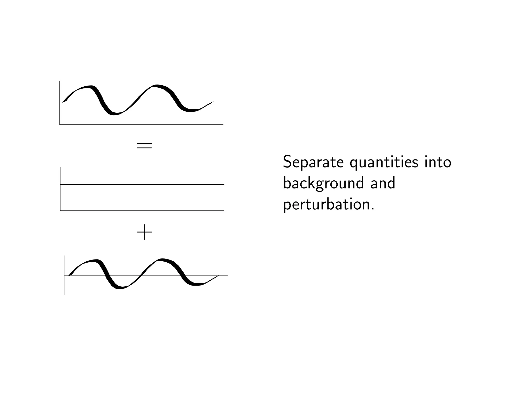
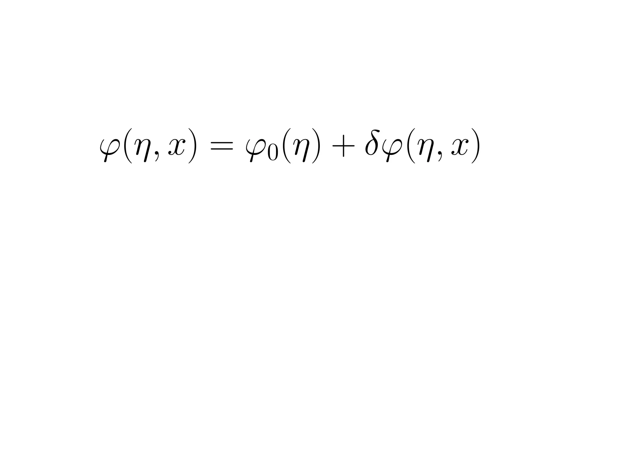
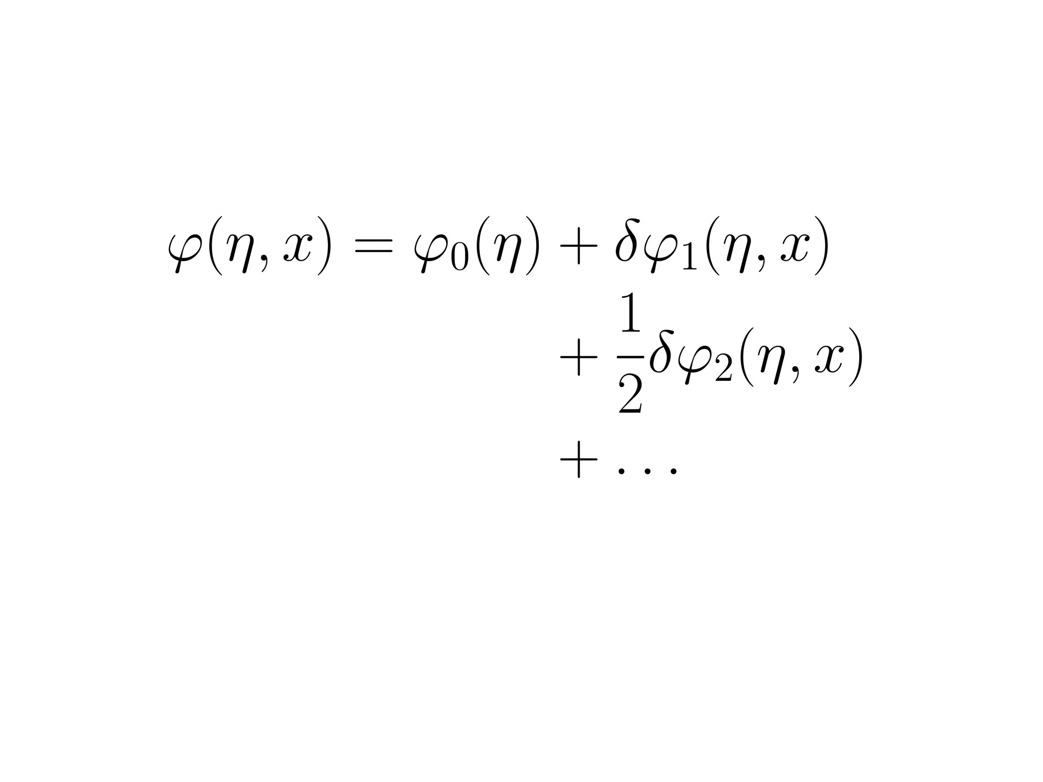
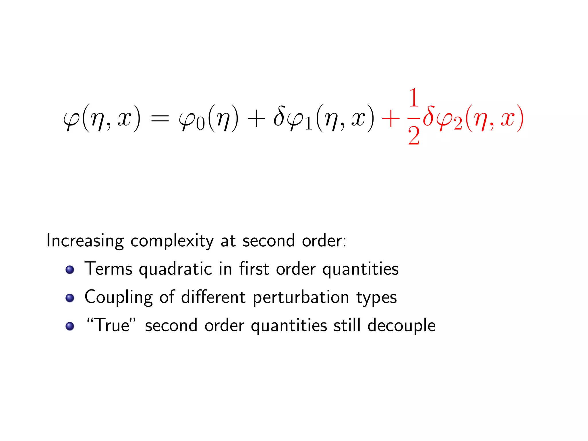
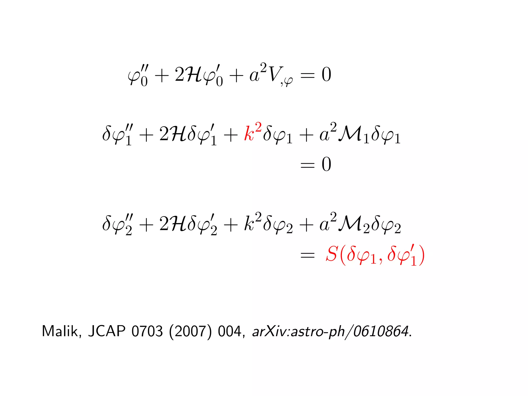
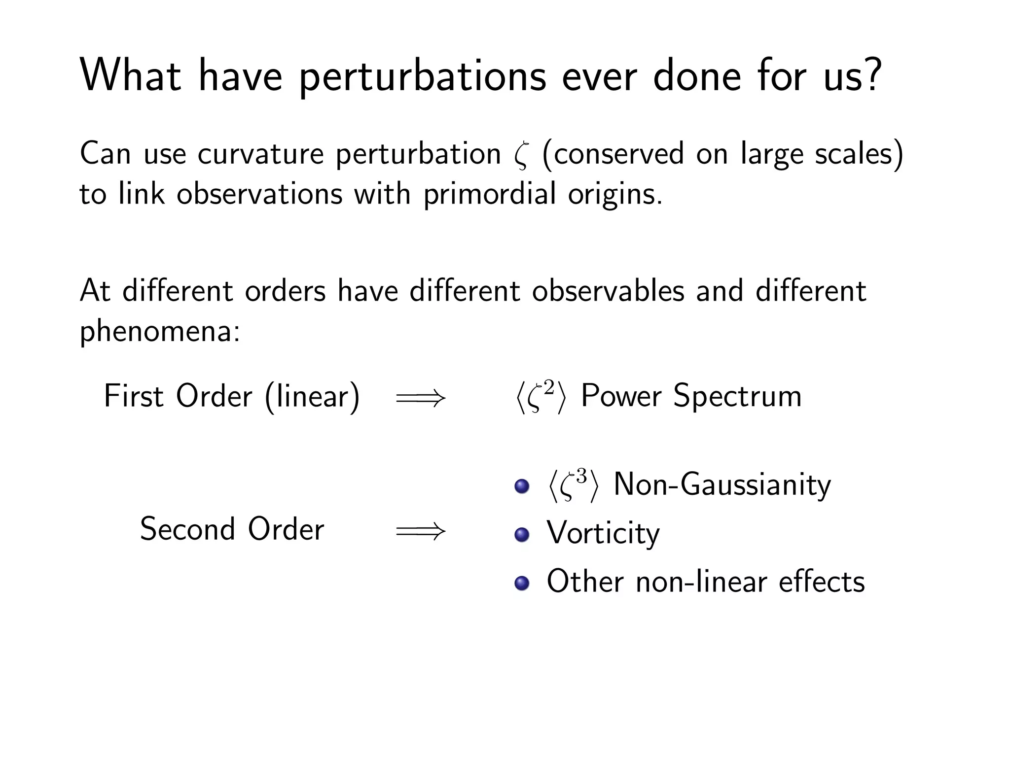
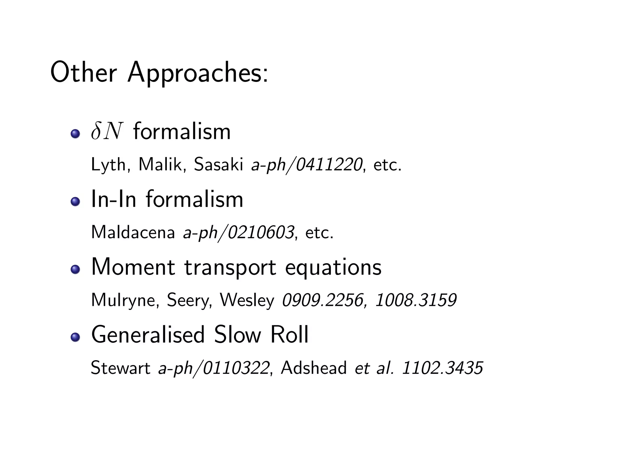
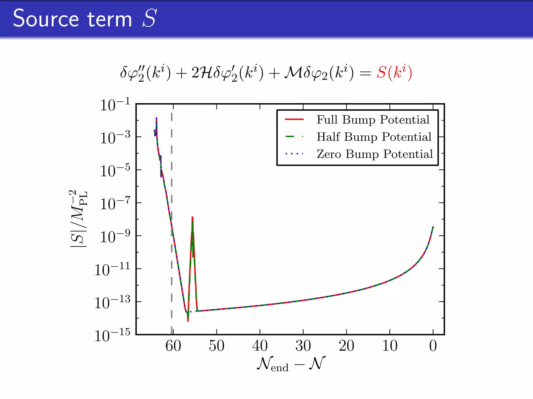
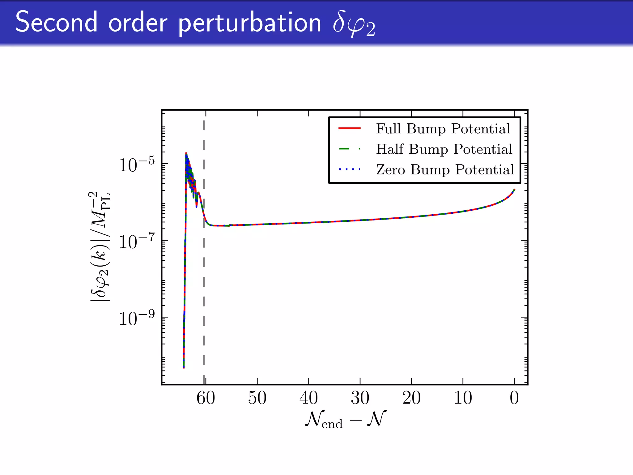
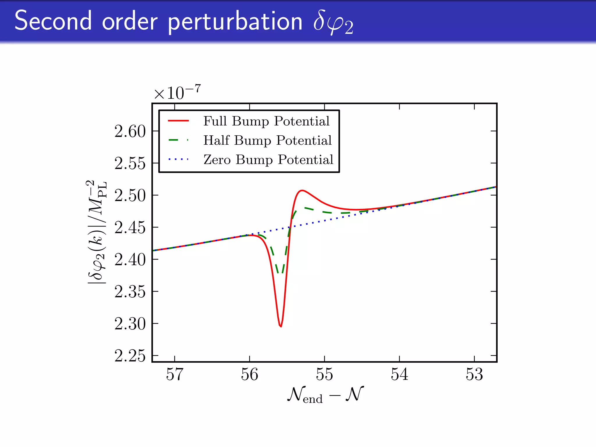
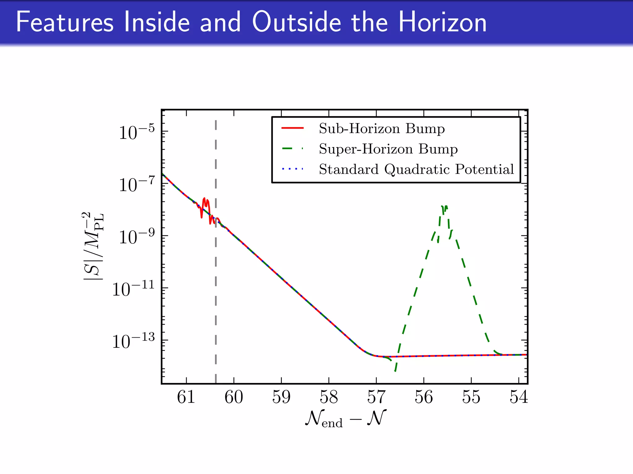
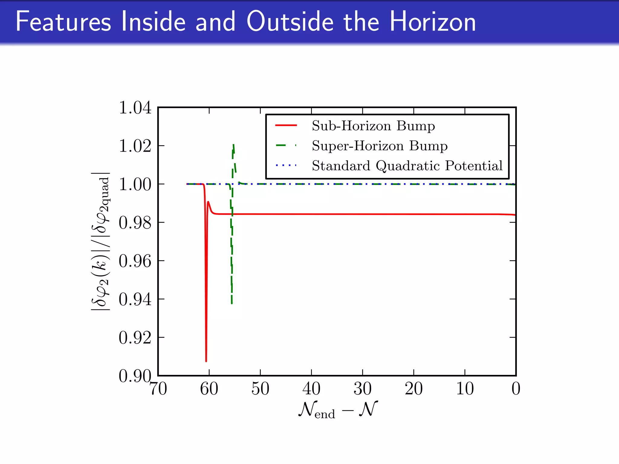
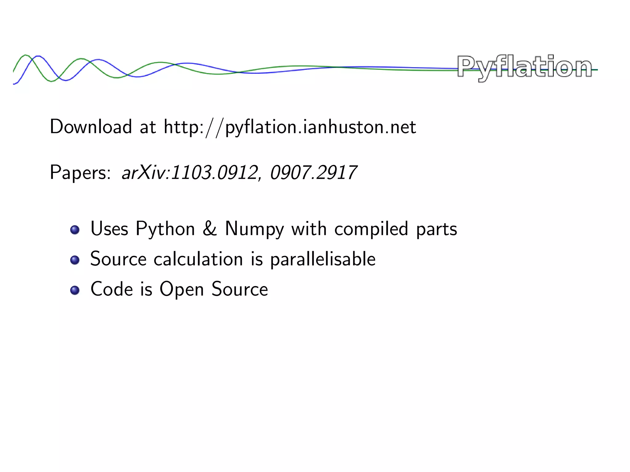
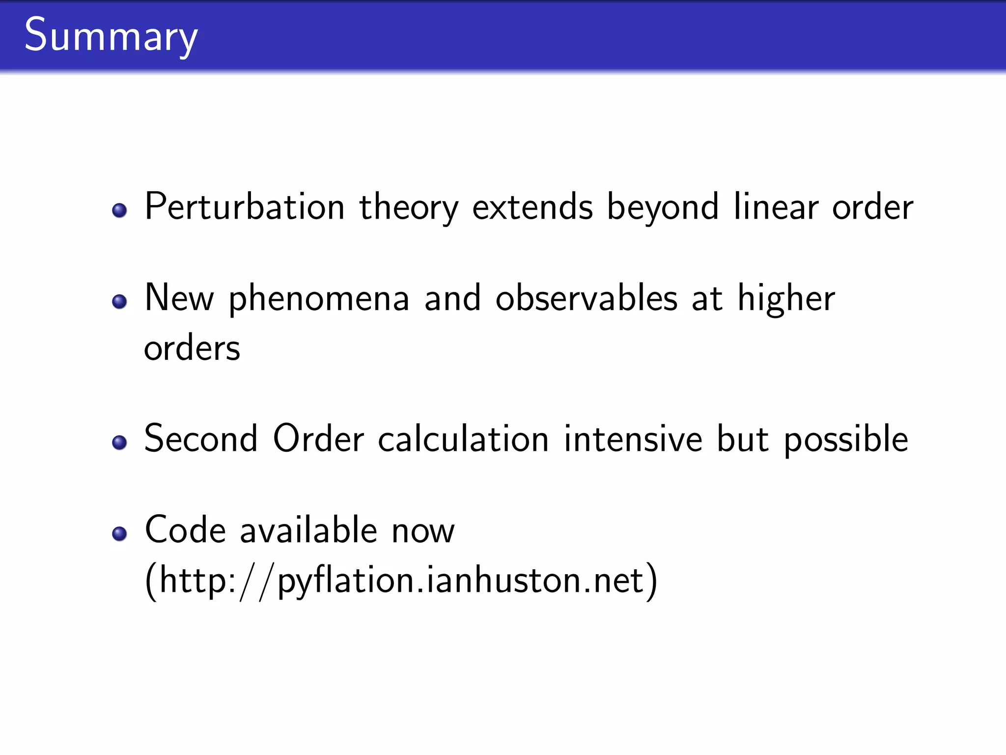
This document outlines research on second-order perturbations during inflation beyond the slow-roll approximation. It discusses perturbation theory at first and second order, and presents results on the source term and second-order perturbations for inflation models with features. The document also describes Pyflation, an open-source Python code for numerically calculating inflationary perturbations up to second order, and outlines future goals for the code including calculating the three-point function and incorporating multi-field models.

1. Second Order Perturbations During
Inflation Beyond Slow-roll
Ian Huston
Astronomy Unit, Queen Mary, University of London
IH, K.A.Malik, arXiv:1103.0912 and 0907.2917 (JCAP 0909:019)
Software available at http://pyflation.ianhuston.net

2. Outline
1
Perturbation Theory
1st and 2nd Order Perturbations, Gauge Invariance
2
Our Results
Source term and Second Order results for feature models
3
Our Code
Implementation, properties and future goals

3. Outline
1
Perturbation Theory
1st and 2nd Order Perturbations, Gauge Invariance
2
Our Results
Source term and Second Order results for feature models
3
Our Code
Implementation, properties and future goals

4. Outline
1
Perturbation Theory
1st and 2nd Order Perturbations, Gauge Invariance
2
Our Results
Source term and Second Order results for feature models
3
Our Code
Implementation, properties and future goals

5. Outline
1
Perturbation Theory
1st and 2nd Order Perturbations, Gauge Invariance
2
Our Results
Source term and Second Order results for feature models
3
Our Code
Implementation, properties and future goals

6. Faucher-Gigure et al., Science 2008

7. perturbations
Long review: Malik & Wands 0809.4944
Short technical review: Malik & Matravers 0804.3276

8. Separate quantities into
background and
perturbation.

9. ϕ(η, x) = ϕ0(η) + δϕ(η, x)
1
+ δϕ2(η, x)
2

10. ϕ(η, x) = ϕ0(η) + δϕ1(η, x)
1
+ δϕ2(η, x)
2
+ ...

11. Gauge Choice Required
Background split not covariant
Many possible descriptions
Should give same physical answers!
⇒ Use Gauge Invariant Variables

12. Gauge Choice Required
Background split not covariant
Many possible descriptions
Should give same physical answers!
⇒ Use Gauge Invariant Variables

13. First order transformation
xµ → xµ + ξ µ
between gauges
µ
ξ1 = (α1, β1,i + γ1)
i
+
T1 = T1 + £ξ1 T0
⇓
δϕ1 = δϕ1 + ϕ0α1

14. Perturbed flat FRW metric at first order
g00 = −a2 (1 + 2φ1 )
g0i = a2 (B1,i − S1i )
gij = a2 (1 − 2ψ)γij + 2E1,ij + 2F1(i,j) + h1ij
Bardeen 1980

15. Perturbed flat FRW metric at first order
g00 = −a2 (1 + 2φ1 )
g0i = a2 (B1,i − S1i )
gij = a2 (1 − 2ψ)γij + 2E1,ij + 2F1(i,j) + h1ij
Bardeen 1980

16. Perturbed flat FRW metric at first order
g00 = −a2 (1 + 2φ1 )
g0i = a2 (B1,i )
gij = a2 (1 − 2ψ)δij + 2E1,ij
Bardeen 1980

17. Choosing a gauge
Longitudinal: zero shear
Comoving: zero 3-velocity
Flat: zero curvature
Uniform density: zero energy density
...

18. Example for Flat gauge:
Metric transformation: ψ1 = ψ1 − Hα1
Flat gauge: α1 = ψ1 /H
Scalar transformation: δϕ1 = δϕ1 + ϕ0 α1
Result
ψ1
δϕ1 flat = δϕ1 + ϕ0
H
Sasaki 1986, Mukhanov 1988

19. Well-known gauge invariant variables
ζ = ψ1 + H δρ1 Curvature perturbation on uniform
ρ0
density hypersurfaces
R = ψ1 − H(v1 + B1 ) Curvature perturbation on comoving
hypersurfaces
Ψ = ψ1 − H(B1 − E1 ) Curvature perturbation on zero shear
hypersurfaces (longitudinal gauge)

20. 1
ϕ(η, x) = ϕ0(η) + δϕ1(η, x) + δϕ2(η, x)
2
Increasing complexity at second order:
Terms quadratic in first order quantities
Coupling of different perturbation types
“True” second order quantities still decouple

21. δGµν = 8πGδTµν
⇓
Eqs of Motion

22. ϕ0 + 2Hϕ0 + a2 V,ϕ = 0
δϕ1 + 2Hδϕ1 + k 2 δϕ1 + a2 M1 δϕ1
=0
δϕ2 + 2Hδϕ2 + k 2 δϕ2 + a2 M2 δϕ2
= S(δϕ1 , δϕ1 )
Malik, JCAP 0703 (2007) 004, arXiv:astro-ph/0610864.

23. ϕ0 + 2Hϕ0 + a2 V,ϕ = 0
δϕ1 + 2Hδϕ1 + k 2 δϕ1 + a2 M1 δϕ1
=0
δϕ2 + 2Hδϕ2 + k 2 δϕ2 + a2 M2 δϕ2
= S(δϕ1 , δϕ1 )
Malik, JCAP 0703 (2007) 004, arXiv:astro-ph/0610864.

24. ϕ0 + 2Hϕ0 + a2 V,ϕ = 0
δϕ1 + 2Hδϕ1 + k 2 δϕ1 + a2 M1 δϕ1
=0
δϕ2 + 2Hδϕ2 + k 2 δϕ2 + a2 M2 δϕ2
= S(δϕ1 , δϕ1 )
Malik, JCAP 0703 (2007) 004, arXiv:astro-ph/0610864.

25. What have perturbations ever done for us?
Can use curvature perturbation ζ (conserved on large scales)
to link observations with primordial origins.
At different orders have different observables and different
phenomena:
First Order (linear) =⇒ ζ 2 Power Spectrum
ζ 3 Non-Gaussianity
Second Order =⇒ Vorticity
Other non-linear effects

26. Other Approaches:
δN formalism
Lyth, Malik, Sasaki a-ph/0411220, etc.
In-In formalism
Maldacena a-ph/0210603, etc.
Moment transport equations
Mulryne, Seery, Wesley 0909.2256, 1008.3159
Generalised Slow Roll
Stewart a-ph/0110322, Adshead et al. 1102.3435

27. results
Second Order Perturbations During Inflation Beyond Slow-roll,
Huston & Malik, arXiv:1103.0912
2nd order equations: Malik, arXiv:astro-ph/0610864

28. Bump Potential
1 ϕ − ϕb
Vb (ϕ) = m2 ϕ2 1 + c sech
2 d
Chen et al. arXiv:0801.3295 etc.
Transient breaking of slow roll around feature
Asymptotes to quadratic potential away from feature
Demonstrated step potential in paper
Plots show result for WMAP pivot scale.
X-axis is efolds remaining until end of inflation.

29. Breaking Slow Roll
2
0
−2
ηV
−4
−6 Step Potential
Bump Potential
Standard Quadratic Potential
−8
57 56 55 54 53
Nend − N

30. First Order Power Spectrum
10−2
Full Bump Potential
Half Bump Potential
Zero Bump Potential
−1/2
10−3
k 3/2 |δϕ1 |/MPL
10−4
10−5
60 50 40 30 20 10 0
Nend − N

31. First Order Power Spectrum
×10−5
3.1
−1/2
k 3/2 |δϕ1 |/MPL
3.0
2.9
2.8 Full Bump Potential
Half Bump Potential
Zero Bump Potential
2.7
57 56 55 54 53
Nend − N

32. Source term S
δϕ2 (k i ) + 2Hδϕ2 (k i ) + Mδϕ2 (k i ) = S(k i )
10−1
Full Bump Potential
10−3 Half Bump Potential
Zero Bump Potential
10−5
−2
|S|/MPL
10−7
10−9
10−11
10−13
10−15
60 50 40 30 20 10 0
Nend − N

33. Second order perturbation δϕ2
Full Bump Potential
Half Bump Potential
10−5 Zero Bump Potential
−2
|δϕ2 (k)|/MPL
10−7
10−9
60 50 40 30 20 10 0
Nend − N

34. Second order perturbation δϕ2
×10−7
Full Bump Potential
2.60 Half Bump Potential
2.55 Zero Bump Potential
−2
|δϕ2 (k)|/MPL
2.50
2.45
2.40
2.35
2.30
2.25
57 56 55 54 53
Nend − N

35. Features Inside and Outside the Horizon
10−5 Sub-Horizon Bump
Super-Horizon Bump
Standard Quadratic Potential
10−7
−2
|S|/MPL
10−9
10−11
10−13
61 60 59 58 57 56 55 54
Nend − N

36. Features Inside and Outside the Horizon
1.04
Sub-Horizon Bump
1.02 Super-Horizon Bump
Standard Quadratic Potential
|δϕ2 (k)|/|δϕ2quad |
1.00
0.98
0.96
0.94
0.92
0.90
70 60 50 40 30 20 10 0
Nend − N

37. code():
First Order Numerical Reviews: Salopek et al. PRD40 1753,
Martin & Ringeval a-ph/0605367

38. Download at http://pyflation.ianhuston.net
Papers: arXiv:1103.0912, 0907.2917
Uses Python & Numpy with compiled parts
Source calculation is parallelisable
Code is Open Source

39. Pyflation uses Python
Quick and easy development
Boost performance using Cython or linking C/Fortran libs
Open Source (can see implementation)
One easy way to get started:
Enthought Python Distribution
http://www.enthought.com
(free for academic use)

40. Pyflation is Open Source
Pyflation is released under the (modified) BSD-license.
Benefits of open source code for scientific projects:
Source code is available for inspection and testing
Code can be modified and re-used
Guaranteed to remain freely accessible

41. Pyflation is parallelisable
k j qj δϕ1(q i)δϕ1(k i − q i)d3q
Numerically intensive calculation
Can be easily parallelised by timestep
Can also single out wavenumber of interest

42. Progress
Single field slow roll
Single field full equation
Multi-field calculation (underway)

43. Implementation
Four Stages:
1 Run background system to find end of inflation
2 Run first order system for range of wavemodes
3 Calculate source term convolution integral
4 Run second order system with source term
Paper plots created with
Results are saved in HDF5 files Matplotlib

44. Future Plans
Three-point function of δϕ
Using Green’s function solution from Seery, Malik, Lyth
arXiv:0802.0588
Multi-field equation
Could check δN predictions, ζ conservation etc.
Tensor & Vorticity similarities
Similar equations of motion in other non-linear processes

45. Future Plans
Three-point function of δϕ
Using Green’s function solution from Seery, Malik, Lyth
arXiv:0802.0588
Multi-field equation
Could check δN predictions, ζ conservation etc.
Tensor & Vorticity similarities
Similar equations of motion in other non-linear processes

46. Future Plans
Three-point function of δϕ
Using Green’s function solution from Seery, Malik, Lyth
arXiv:0802.0588
Multi-field equation
Could check δN predictions, ζ conservation etc.
Tensor & Vorticity similarities
Similar equations of motion in other non-linear processes

47. Other interesting non-linear processes
Vorticity generation
(Half-day Vorticity meeting in RAS 14th July)
Magnetic field generation
2nd order Gravitational waves

48. Summary
Perturbation theory extends beyond linear order
New phenomena and observables at higher
orders
Second Order calculation intensive but possible
Code available now
(http://pyflation.ianhuston.net)

49. i i 2 i 2 8πG 2 8πG i
δϕ2 (k ) + 2Hδϕ2 (k ) + k δϕ2 (k ) + a V,ϕϕ + 2ϕ0 V,ϕ + (ϕ0 ) V0 δϕ2 (k )
H H
1 3 3 3 i i i 16πG i i 2 i i
+ d pd qδ (k − p − q ) Xδϕ1 (p )δϕ1 (q ) + ϕ0 a V,ϕϕ δϕ1 (p )δϕ1 (q )
(2π)3 H
8πG 2
2 i i i i
+ ϕ0 2a V,ϕ ϕ0 δϕ1 (p )δϕ1 (q ) + ϕ0 Xδϕ1 (p )δϕ1 (q )
H
4πG 2 ϕ X
0 i i i i i
−2 Xδϕ1 (k − q )δϕ1 (q ) + ϕ0 δϕ1 (p )δϕ1 (q )
H H
4πG i i 2 8πG i i
+ ϕ0 δϕ1 (p )δϕ1 (q ) + a V,ϕϕϕ + ϕ0 V,ϕϕ δϕ1 (p )δϕ1 (q )
H H
1 3 3 3 i i i 8πG pk q k i i i
+ d pd qδ (k − p − q ) 2 δϕ1 (p ) Xδϕ1 (q ) + ϕ0 δϕ1 (q )
(2π)3 H q2
 
2 16πG i i 4πG 2 ϕ
0 pi qj kj ki
+p δϕ1 (p )ϕ0 δϕ1 (q ) + p q l −  ϕ δϕ (ki − q i )ϕ δϕ (q i )
l 0 1 0 1
H H H k2
X 4πG 2 p q l p q m + p2 q 2
l m i i i
+2 ϕ0 δϕ1 (p ) Xδϕ1 (q ) + ϕ0 δϕ1 (q )
H H k2 q 2
4πG q 2 + pl q l i i l i i
+ 4X δϕ1 (p )δϕ1 (q ) − ϕ0 pl q δϕ1 (p )δϕ1 (q )
H k2
4πG pl q l pm q m
2 ϕ
0 i i i i
+ Xδϕ1 (p ) + ϕ0 δϕ1 (p ) Xδϕ1 (q ) + ϕ0 δϕ1 (q )
H H p2 q 2
 
ϕ0 pl q l + p2 2 i i q 2 + pl q l i i
+ 8πG  q δϕ1 (p )δϕ1 (q ) − δϕ1 (p )δϕ1 (q )
H k2 k2
4πG 2 kj k pi pj
i i i i
+ 2 Xδϕ1 (p ) + ϕ0 δϕ1 (p ) Xδϕ1 (q ) = 0
H k2 p2